Three-Dimensional Magnetotelluric Inversion for Triaxial Anisotropic Medium in Data Space

Abstract

The interpretation of three-dimensional (3-D) magnetotelluric (MT) data is usually based on the isotropic assumption of the subsurface structures, and this assumption could lead to erroneous interpretation in the area with considerable electrical anisotropy. Although arbitrary anisotropy is much closer to the ground truth, it is generally more challenging to recover full anisotropy parameters from 3-D inversion. In this paper, we present a 3-D triaxial anisotropic inversion framework using the edge-based finite element method with a tetrahedral mesh. The 3-D inverse problem is solved by the Gauss-Newton (GN) method which shows fast convergence behavior. The computation cost of the data-space method depends on the size of data, which is usually smaller than the size of model; therefore, we transform the inversion algorithm from the model space to the data space for memory efficiency. We validate the effectiveness and applicability of the developed algorithm using several synthetic model studies.

1. Introduction

With the fast development of computer hardware and numerical algorithm, 3-D magnetotelluric (MT) inversion has been widely used in many applications, such as mineral exploration [1,2], deep earth structure imaging [3,4,5], and geothermal exploration [6,7].

At present, the interpretation of magnetotelluric data is generally based on the isotropy assumption of the Earth’s geoelectric structure, but numerous studies have revealed the prevalence of electrical anisotropy in the Earth [8,9,10]. This electric anisotropy can affect the magnetotelluric response [11,12]. If the isotropic inversion technique was adopted to invert the data affected by electrical anisotropy, it could produce artifacts and even lead to erroneous interpretation [13,14]. Although the arbitrary anisotropy assumption is much closer to the ground truth, it needs to consider more model parameters compared to the isotropic inversion. Moreover, it is more challenging to solve the arbitrary anisotropy inversion due to the strong non-uniqueness [15].

The current research of anisotropic MT inversion mainly focuses on two-dimension (2-D) inversion and 3-D triaxial inversion in the model space. Li et al. (2003) implemented 2-D anisotropic inversion using the Gauss-Newton method [16]. Pek et al. (2011) used the nonlinear conjugate gradient (NLCG) method to solve 2-D arbitrary anisotropic inversion, and they found that it is challenging to reconstruct the anisotropic dipping angle without additional a priori information [17]. Yu et al. (2022) reported 2-D arbitrary anisotropic MT inversion using the limited-memory quasi-Newton (Q-N) method [18]. For 3-D anisotropic inversion, Cao et al. (2018) and Wang et al. (2021) realized 3-D magnetotelluric inversion with triaxial anisotropy using the limited-memory Broyden–Fletcher–Goldfarb–Shanno (L-BFGS) method [15,19]. Kong et al. (2022) reported 3-D arbitrary anisotropic MT inversion using the NLCG method [20]. These published results are based on the model-space algorithm, and the memory consumption depends on the size of model. Considering the number of model parameters is relatively large for 3-D inversion, the iterative solver is usually used to solve the model update in each inversion iteration.

We develop a 3-D triaxial anisotropic inversion scheme using the data space method, and the Gauss–Newton method is used to solve this inversion problem. To accurately simulate the rugged topography and complex geoelectric structures, the unstructured tetrahedral mesh is used to discretize the computational domain. For simplicity, we now only consider three principal resistivities. The anisotropic strike can be determined by the phase tensor technique and induction arrows in some cases [21,22], and also by considering the known geological information. At present, it is still challenging to resolve the anisotropic dip and slant using the current inversion strategy. The anisotropic inversion algorithm is transformed from the model space to the data space to reduce the memory requirement [23,24,25,26]. Moreover, the direct solver is used to solve the normal equation in each inversion iteration. Compared to the iterative solver, the direct solver can improve the stability of the inversion process.

In this paper, we first introduce the anisotropic forward modeling with a secondary field formulation. Following this, we describe the triaxial anisotropic inversion based on the Gauss–Newton optimization in the data space. Finally, we demonstrate the effectiveness and applicability of the developed algorithm using several synthetic models.

2. Basic Theory

2.1. 3-D Magnetotelluric Forward Modeling with a Secondary Field Formulation

We start from Maxwell’s equations and assume the time dependence term of $e^{i\omega t}$. By ignoring the displacement current, we can obtain the diffusion equation as follows:

$$\nabla \times \nabla \times E^s+i\omega {\mu }_0\widehat{\sigma }{E}^s=-i\omega {\mu }_0\left(\widehat{\sigma }-{\sigma }_p\right)E^p,$$

(1)

where $E^s$ and $E^p$ are the secondary field and the primary field, respectively; $\omega$ is the angular frequency; ${\mu }_0$ is the free space magnetic permeability; ${\sigma }_p$ is the background conductivity, and $\widehat{\sigma }$ is the anisotropic conductivity tensor, described as follows [27]:

$$\widehat{\sigma }=R_z\left(-{\alpha }_S\right)R_x\left(-{\alpha }_D\right)R_z\left(-{\alpha }_L\right)\left[\begin{array}{ccc}{\sigma }_x& & \\ & {\sigma }_y& \\ & & {\sigma }_z\end{array}\right]R_z\left({\alpha }_S\right)R_x\left({\alpha }_D\right)R_z\left({\alpha }_L\right),$$

(2)

where ${\sigma }_x$, ${\sigma }_y,$ and ${\sigma }_z$ are three principal conductivities in the X, Y, and Z directions, respectively; ${\alpha }_S$, ${\alpha }_D$, and ${\alpha }_L$ are the anisotropic strike, dip, and slant, respectively; and $R_z\left({\alpha }_S\right)$, $R_x\left({\alpha }_D\right),$ and $R_z\left({\alpha }_L\right)$ represent the rotations around the Z axis and X axis through the angle ${\alpha }_S$, ${\alpha }_D$ and ${\alpha }_L$, respectively.

The large sparse system of linear equations can be obtained by applying finite element analysis:

$$A{E}^s=b.$$

(3)

The Dirichlet boundary condition is adopted for solving the above equation by assuming the secondary electrical field vanishes on the boundary of the modeling domain. We use the tetrahedral mesh to discretize the computational domain. Compared to the total field formulation, one has to select proper background conductivity when simulating models with complex topography using the secondary field formulation. We solve Equation (3) using the parallel direct solver MKL Paradiso [28]. Considering the independence of frequency, we further parallelize the forward modeling algorithm over the frequencies to speed up the computation.

2.2. Data-Space Inversion Theory for Triaxial Anisotropic Medium

For the triaxial anisotropic inversion, three anisotropic rotation angles are constant, and the objective functional can be written as:

$$\phi \left(m\right)={\phi }_d\left(m\right)+{\beta }_x{\phi }_x\left(m_x\right)+{\beta }_y{\phi }_y\left(m_y\right)+{\beta }_z{\phi }_z\left(m_z\right).$$

(4)

where ${\phi }_d\left(m\right)$ is the data misfit; ${\phi }_x\left(m_x\right)$, ${\phi }_y\left(m_y\right),$ and ${\phi }_z\left(m_z\right)$ are the model regularization term in the X, Y, and Z directions, respectively; $m={\left(\begin{array}{ccc}{m}_x& m_y& m_z\end{array}\right)}^T$ is the model parameter and $m_x=ln{\sigma }_x$, $m_y=ln{\sigma }_y,$ and $m_z=ln{\sigma }_z$ are the model parameters in three principal directions; and ${\beta }_x$, ${\beta }_y,$ and ${\beta }_z$ are the regularization parameters which are used to balance the data fitting and model constraints.

The data misfit term is described as:

$${\phi }_d\left(m\right)=\parallel W_d{\left(d^{pre}-d^{obs}\right)\parallel }^2,$$

(5)

where $d^{pre}=F\left(m\right)$ is the predicted data, $F$ is the forward modeling operator, and $d^{obs}$ represents the observed data. $W_d$ is the diagonal data weighting matrix, which is constructed based on the reciprocal of the standard error of the observed data, and the readers can refer to Appendix A for more details.

The model regularization term along each principal direction can be written as:

$${\phi }_i=\parallel L_i{\left(m_i-m_i^{ref}\right)\parallel }^2,i=x,y,z,$$

(6)

where $m_i^{ref}$ is reference model parameter; and $L_x, L_y,$ and $L_z$ are the model roughness matrices for the conductivities in the X, Y, and Z directions, respectively. We adopted a method similar to Cai et al., 2021, to calculate the roughness matrix. We can control the smoothness of the inverted model by choosing the number of adjacent elements [29,30]. The roughness matrix can stabilize the inversion by providing a measure of model variations and avoiding spurious structures [31].

The Gauss–Newton method is used to minimize the objective functional, and we solve the normal equation in each Gauss–Newton iteration to obtain the model update:

$$\begin{array}{l}\left[Re\left\{{\left(W_{d}J\right)}^H{W}_{d}J\right\}+L^{T}L\right]\delta m\\ \hspace{1em}\hspace{1em}\hspace{1em}\hspace{1em}\hspace{1em}\hspace{1em}\hspace{1em}\hspace{1em}=-\left[Re\left\{{\left(W_{d}J\right)}^H{W}_d\left(d^{pre}-d^{obs}\right)\right\}+L^{T}L\left(m-m^{ref}\right)\right],\end{array}$$

(7)

$$J=\left[J_x,J_y,J_z\right],$$

(8)

$$L=\left[\begin{array}{ccc}\sqrt{{\beta }_x}{L}_x& & \\ & \sqrt{{\beta }_y}{L}_y& \\ & & \sqrt{{\beta }_z}{L}_z\end{array}\right],$$

(9)

$$m^{ref}={\left[m_x^{ref},m_y^{ref},m_z^{ref}\right]}^T,$$

(10)

where $J_x$, $J_y,$ and $J_z$ are the sensitivity matrices for anisotropic inversion; $H$ denotes the Hermitian transpose; and $T$ denotes the transpose.

We transform the system of normal equations from the model space to the data space using the Sherman–Morrison–Woodbury formula [32], and the inverse of the reduced Hessian matrix of Equation (7) can be written as:

$${\left[Re\left\{{\left(W_{d}J\right)}^H{W}_{d}J\right\}+L^{T}L\right]}^{-1}=U^{-1}-U^{-1}D{\Gamma }^{-1}{D}^H{U}^{-1},$$

(11)

$$D=\left[Re\left\{{\left(W_{d}J\right)}^H\right\},Im\left\{{\left(W_{d}J\right)}^H\right\} \right],$$

(12)

$$U=L^{T}L+ϵ·diag\left\{L^{T}L\right\},$$

(13)

$$\Gamma =I+D^H{U}^{-1}D.$$

(14)

where $I$ is an identity matrix, and $ϵ$ is a small positive number, and it is added to Equation (13) to enable the positive definiteness of matrix. Numerical tests show that its influence on the inversion results is negligible [25,26].

We multiply both sides of Equation (7) by the inverse of the reduced Hessian matrix, and substituting Equation (11) into Equation (7) to obtain the system of normal equations in the data space:

$$\delta m=U^{-1}R-U^{-1}D{\Gamma }^{-1}{D}^H{U}^{-1}R,$$

(15)

$$R=-\left[Re\left\{{\left(W_{d}J\right)}^H{W}_d\left(d^{pre}-d^{obs}\right)\right\}+L^{T}L\left(m-m^{ref}\right)\right].$$

(16)

For simplicity, Equation (15) is written as:

$$\delta m=X_1-X_2{X}_3,$$

(17)

$$X_1=U^{-1}R,$$

(18)

$$X_2=U^{-1}D,$$

(19)

$$X_3={\Gamma }^{-1}{D}^H{X}_1.$$

(20)

It is computationally expensive to directly calculate the inverse of matrix $U$. We obtain $X_1$ and $X_2$ by solving the linear equation with $U$ as the coefficient matrix. $U$ is a sparse matrix with the size of $N_m\times N_m$ ($N_m$ is the size of model), and it is efficient to obtain $X_1$ and $X_2$ using the direct solver. We notice that the size of matrix $D$ is $2N_d\times N_m$ ($N_d$ is the size of the data set), and we can solve the matrix $X_2$ by hybrid programming with MPI and OpenMP [33]. The matrix $X_3$ is solved using the direct solver for dense matrix.

The model-space method requires dealing with the sensitivity matrix $J\in {ℂ}^{N_d\times N_m}$ and the dense matrix of ${\left(W_{d}J\right)}^H{W}_{d}J\in {ℂ}^{N_m\times N_m}$. The calculation and storage of the latter term are considerably expensive, and it is generally impractical for the anisotropic inversion. The data-space method deals with matrix $J\in {ℂ}^{N_d\times N_m}$ and $D\in {ℝ}^{2N_d\times N_m}$. Fortunately, these matrices can be stored on the hard disk and some of them can be read into RAM. The matrix of $\Gamma \in {ℝ}^{2N_d\times 2N_d}$ also needs to be stored, but $N_d$ is usually much smaller than $N_m$. Moreover, for the model-space method based on the direct solver, the construction of the coefficient matrix and the right-hand sides of this equation are unsuitable for parallelization. In contrast, most of the solutions of the data space method can be efficiently parallelized.

The regularization parameter is important to obtain geophysical meaningful solutions. We choose the regularization parameters in a similar way as Cai et al., 2021 [30]:

$${\gamma }_i=\frac{\parallel Re\left\{{\left({\mathbf{W}}_d{\mathbf{J}}_i\right)}^H\left({\mathbf{W}}_d{\mathbf{J}}_i\mathbf{x}\right)\right\}{\parallel }_2}{\parallel {\mathbf{L}}_i^T\left({\mathbf{L}}_i\mathbf{x}\right){\parallel }_2},i=x,y,z,$$

(21)

$${\beta }_i=q_i\frac{max\left\{{\gamma }_x,{\gamma }_y,{\gamma }_z\right\}}{n_{iter}^c},i=x,y,z,$$

(22)

where $0<q_i<1$ is an empirical scaling parameter, $n_{iter}$ is the iteration number, and $c$ is a positive integer that is usually less than 3, based on our numerical tests [34]. We have tested the influence of $q_i$ and $c$ on the inversion results as shown in Appendix B.

Once the model update direction $\delta m$ is solved using the data-space method [23], a new model is obtained as:

$$m^{n+1}=m^n+\alpha \delta m^n.$$

(23)

where $\alpha$ is the step length, which ensures the decreasing of the objective functional. An appropriate step length can be obtained by a simple line search strategy [35].

The definition of RMS in this study is given as follows [36]:

$$\mathrm{RMS}=\sqrt{\frac{{\left(W_d\left(d^{pre}-d^{obs}\right)\right)}^T\left(W_d\left(d^{pre}-d^{obs}\right)\right)}{N_d}}.$$

(24)

The workflow for 3-D triaxial anisotropic inversion in data space is shown in Figure 1.

3. Synthetic Model Studies

The developed code is run on the high-performance cluster at China University of Geosciences, Wuhan, China. Each node has 2 Intel Xeon 2.5 GHz CPUs with 20 cores per CPU and 384 GB RAM. We use two cluster nodes in this study. For each node, we set 2 MPI processes and 40 OpenMP threads. The model-space inversion algorithm is solved by the direct solver for dense matrix.

Firstly, we use an example to compare the performance of the model-space and data-space algorithm based on the direct solver. The total number of synthetic observed data is 16,224 (including the real and imaginary parts). We use different discretization to test the performances. The size of models for these different discretization are 20,196, 30,945, 41,280, 61,455, and 82,512, respectively. The memory requirements and CPU time for these models are shown in Figure 2 for the model-space and data-space methods. Although the model-space method is more efficient than the data-space method when the model size is small, the memory consumption and calculation time increase approximately quadratically with the increase of model size for the model-space method. For the data-space method, the memory consumption and computation time increase linearly with the increase of model size. The model-space method easily becomes impractical because the model parameters can be extremely large. Therefore, the data-space method is more feasible for the large-scale anisotropic inversion in certain scenarios.

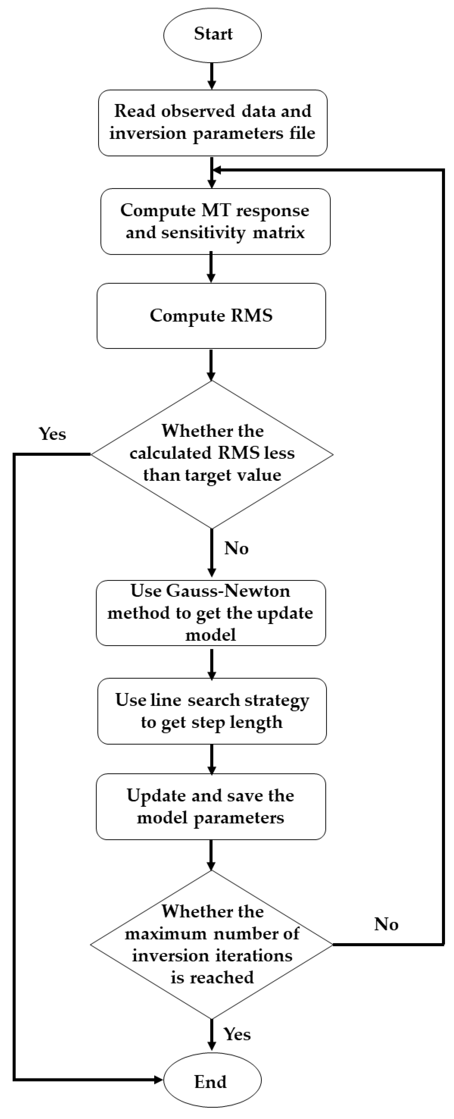
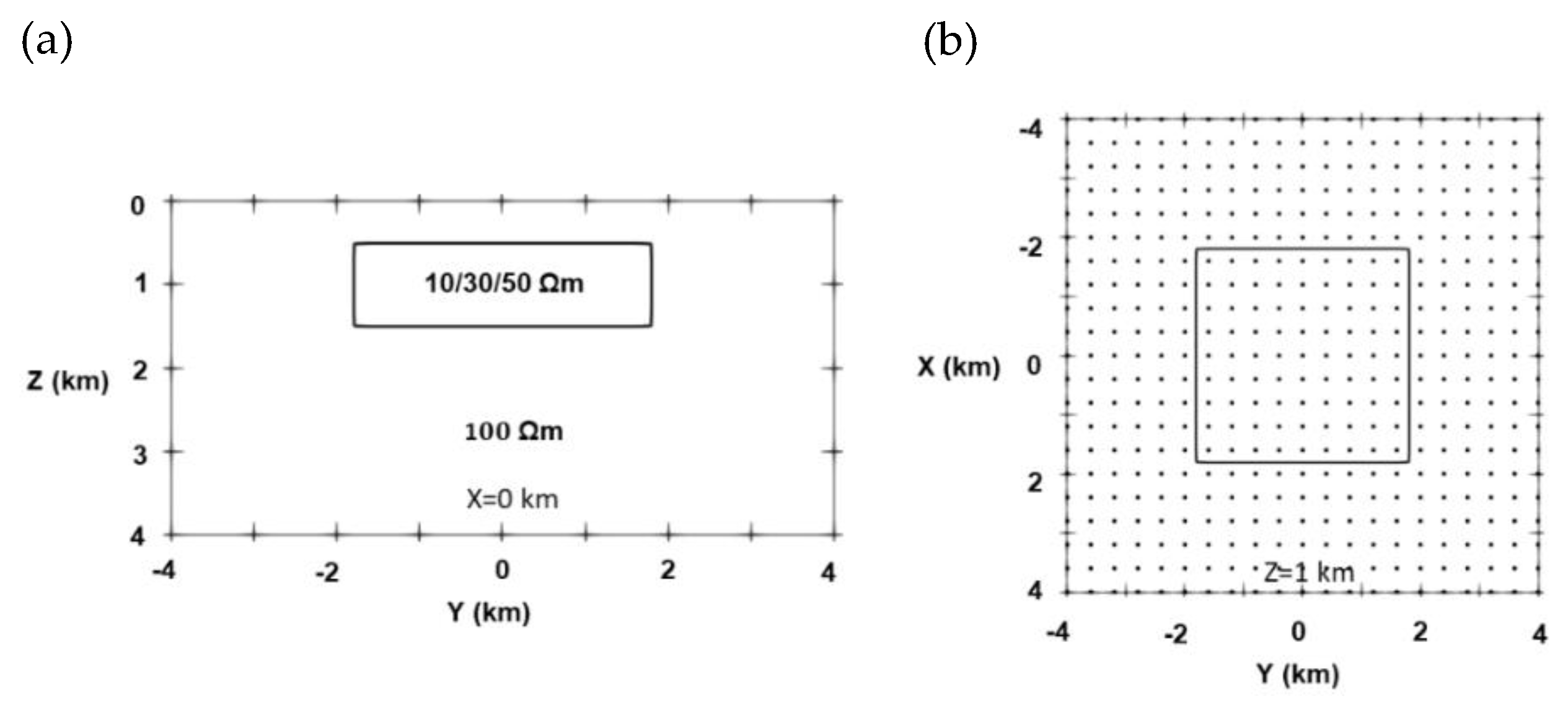
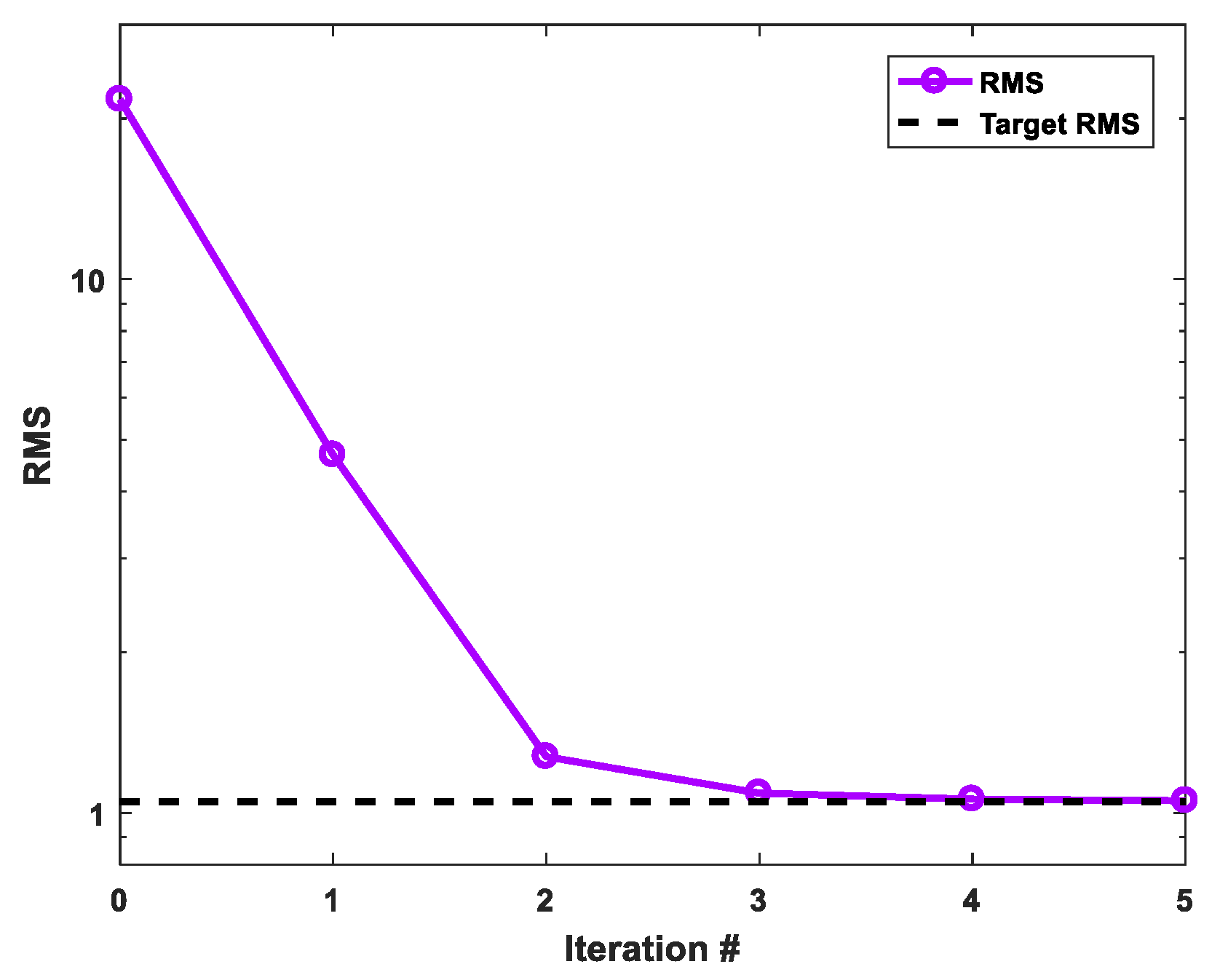
3.1. Algorithm Validation

The SM3 model from Cao et al., 2018 [15] is used to demonstrate the correctness of the developed algorithm, as shown in Figure 3. The anisotropic anomaly with the size of 3.6 km × 3.6 km × 1 km is buried in the homogeneous half-space with a resistivity of $300 \mathsf{\Omega }\mathrm{m}$. The three principal resistivities of the anisotropic block are ${\rho }_x/{\rho }_y/{\rho }_z=10 \mathsf{\Omega }\mathrm{m}/30 \mathsf{\Omega }\mathrm{m}/50 \mathsf{\Omega }\mathrm{m}$, and the values of three rotation angles both are 0. The central location of the anomalous body is (0, 0, 1) km. The resistivity of the air layer is chosen as ${10}^9 \mathsf{\Omega }\mathrm{m}$. We simulate the full impedance tensor data for 5 frequencies (0.1 Hz, 1 Hz, 5 Hz, 10 Hz and 100 Hz) at 169 sites and contaminate the synthetic data by 2% Gauss random noise.

The whole simulation domain for the forward modeling and the inversion are the same, and their size are 40 km × 40 km × 40 km in the X, Y, and Z directions. The thickness of the air layer is 20 km for this model. The forward modeling domain is discretized into 743,603 elements. The inversion domain extends from –4 km to 4 km in the horizontal direction and from 0 km to 4 km in the vertical direction. The mesh of the inversion domain is discretized into 171,370 elements, and the total number of elements in the whole mesh is 480,795. Both the initial model and the reference model are set to be a homogeneous half-space with a resistivity of 50 Ωm. The standard error is set to $0.02·sqrt\left(\left|Z_{xy}·Z_{yx}\right|\right)$. The roughness matrix is calculated using the 20 surrounding elements of each inversion cell. We set the maximum number of iterations to be 10, and the threshold RMS for the inversion is 1.05.

We terminate the inversion after five iterations when the convergence stalls as shown in Figure 4. The RMS rapidly decrease from the initial value of 16.83 to 1.06. The runtime is 9.2 h and the memory consumption is 137.5 GB.

The anisotropic inversion results are shown in Figure 5, Figure 6, Figure 7 and Figure 8. The shape and conductivity values in the anisotropic X and Y directions can be recovered well, and the anisotropic coefficient between the resistivity in the X and Y directions (defined by ${\log }_{10}\left({\rho }_x/{\rho }_y\right)$) is also reasonably recovered. The main source of the magnetotelluric field is the plane wave which propagates vertically. Therefore, the resistivity in the Z direction only has limited influence on the MT response. As a result, the resolution of the recovered vertical resistivity is relatively lower compared to that of the horizontal resistivities. [37]. Our inversion results are in a good agreement with Cao et al., 2018 [15].

The data fitting is shown in Figure 9, we choose the Z_xy and Z_yx components at the frequency of 5 Hz as an example. We can see that the observed data compare well to the predicted data.

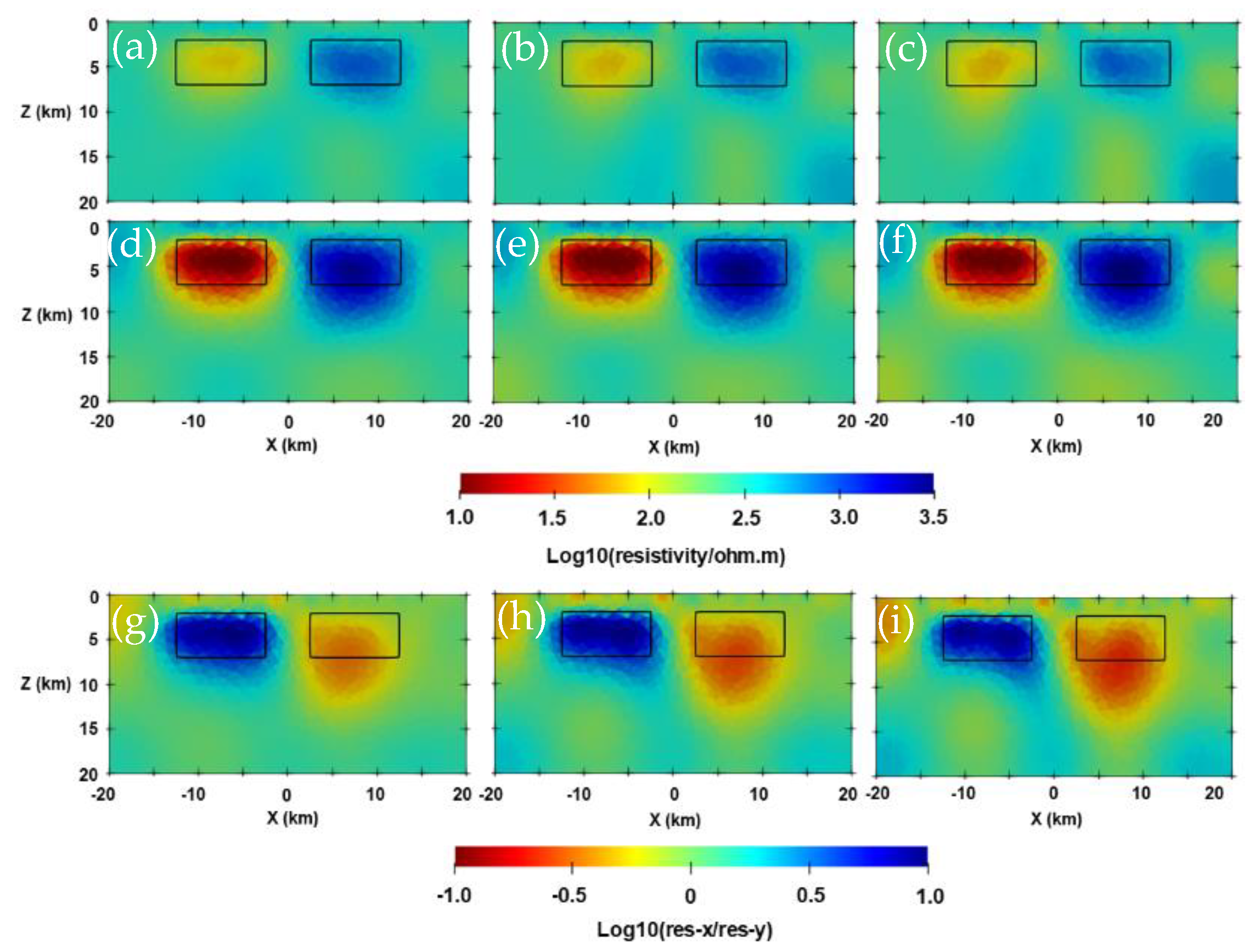
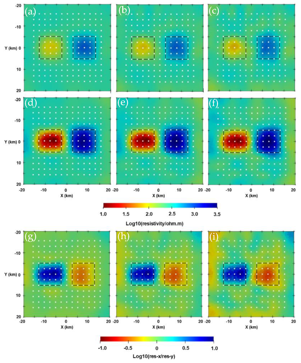
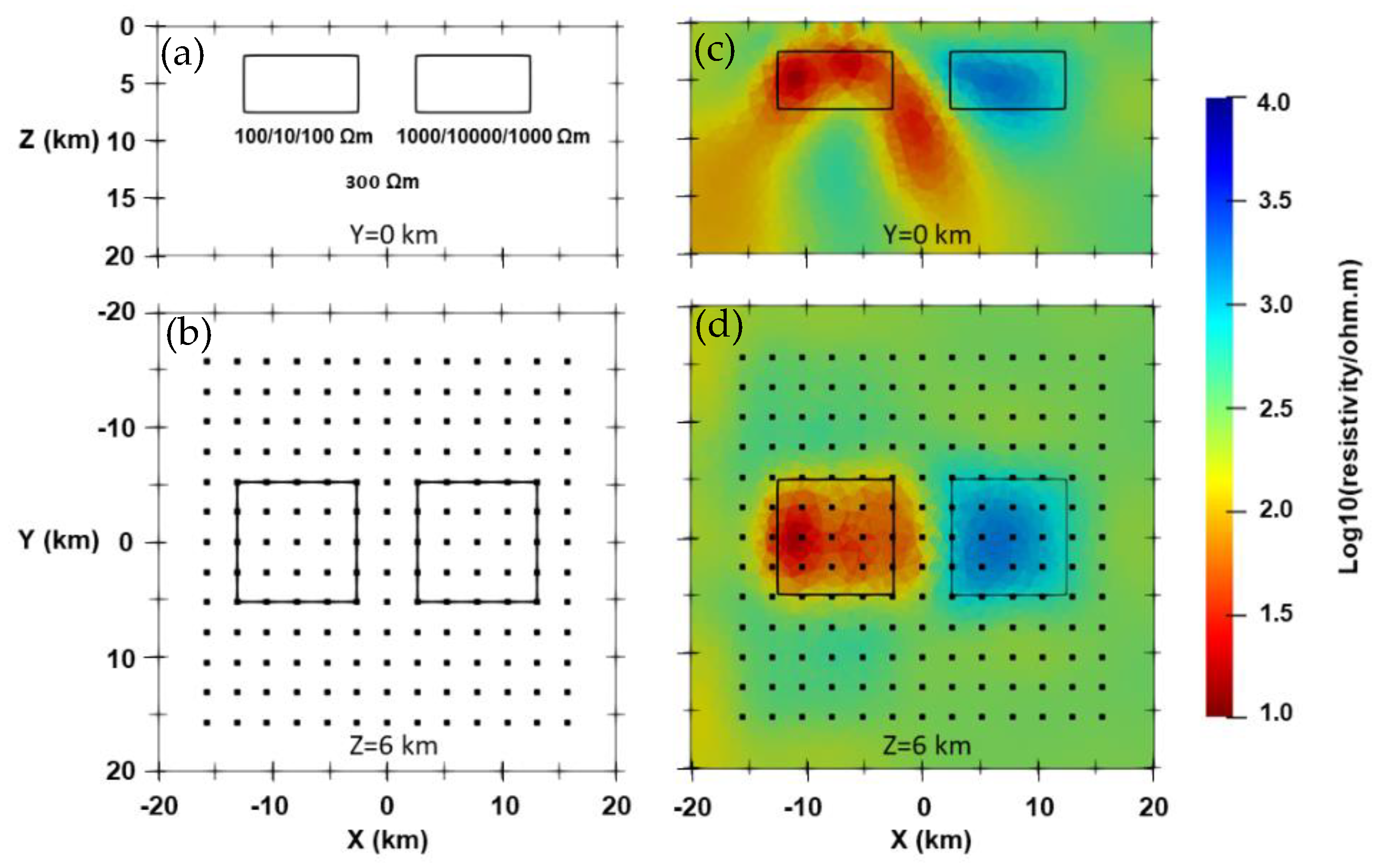
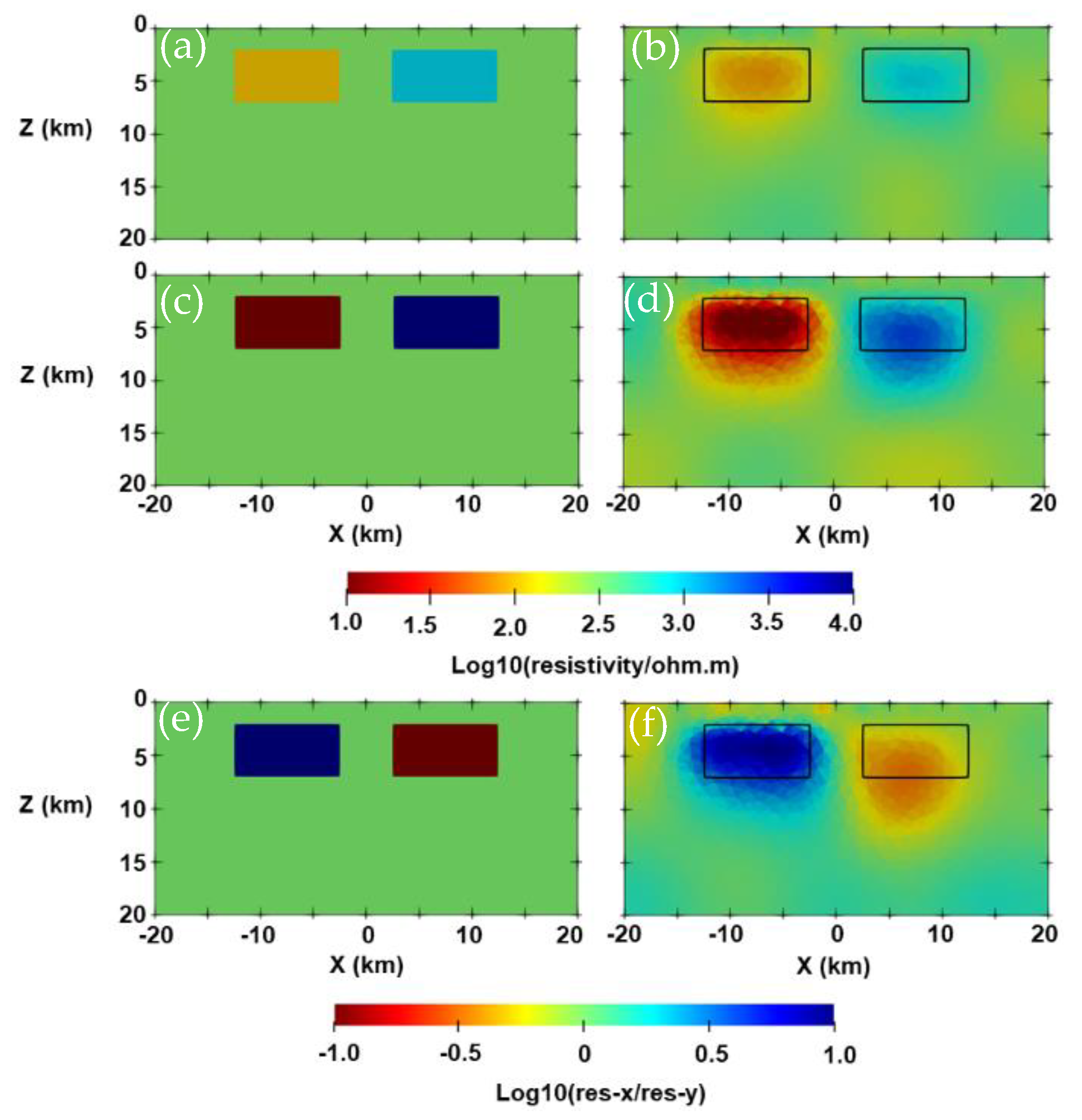
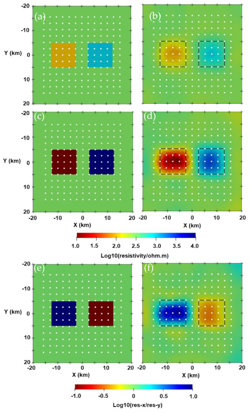
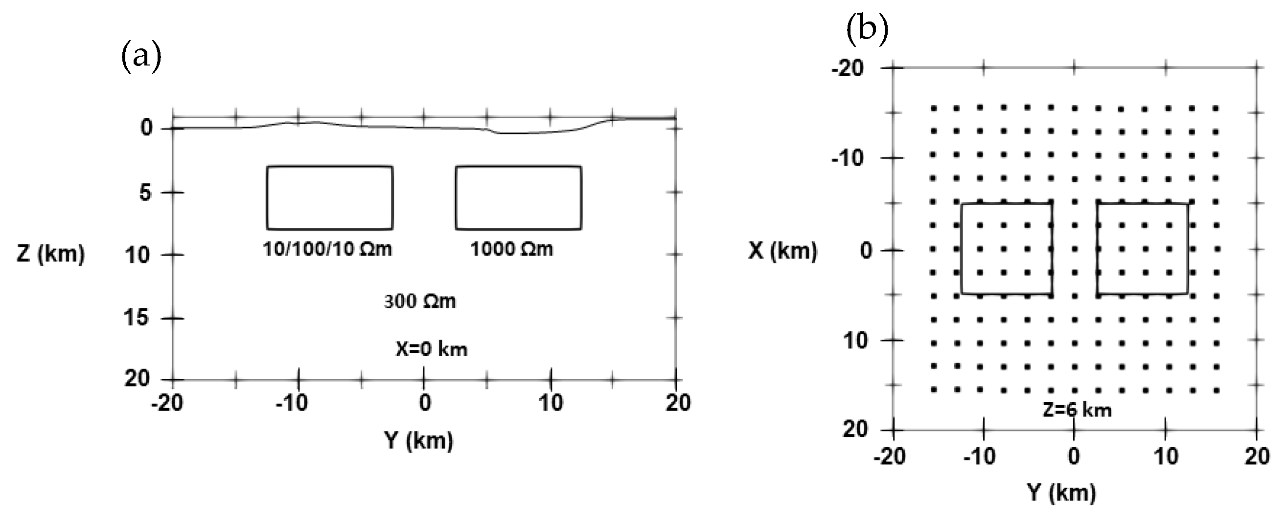
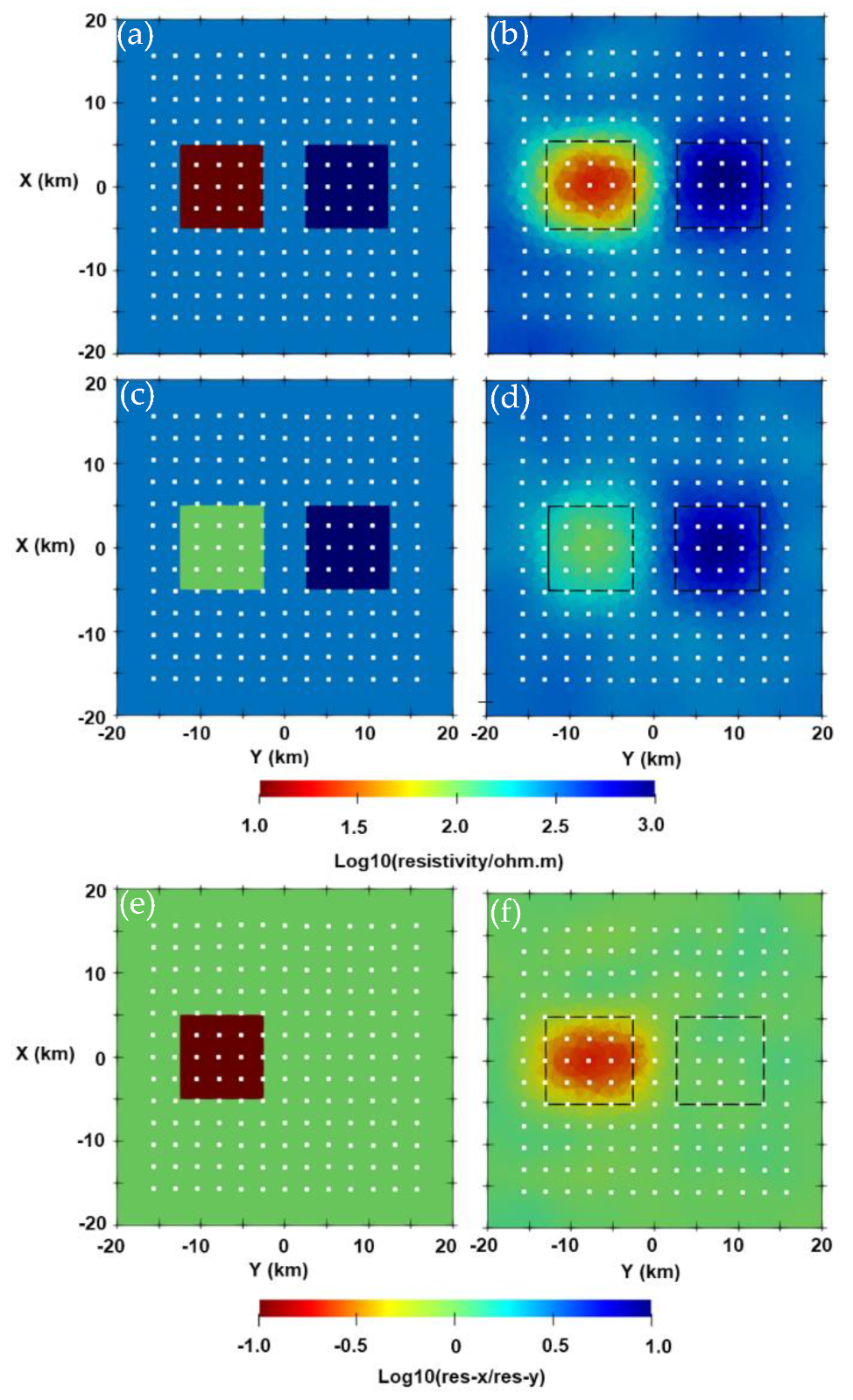
3.2. Two-Blocks Model

To test the effectiveness of our developed inversion algorithm and study the influence of electrical anisotropy, we design a two-blocks model as shown in Figure 10a,b. These two anisotropic anomalies with the resistivities of ${\rho }_x/{\rho }_y/{\rho }_z=100 \mathsf{\Omega }\mathrm{m}/10 \mathsf{\Omega }\mathrm{m}/100 \mathsf{\Omega }\mathrm{m}$ and ${\rho }_x/{\rho }_y/{\rho }_z=1000 \mathsf{\Omega }\mathrm{m}/\mathrm{10,000} \mathsf{\Omega }\mathrm{m}/1000 \mathsf{\Omega }\mathrm{m}$ are embedded in the homogeneous half-space with a resistivity of $300 \mathsf{\Omega }\mathrm{m}$. Both of these anomalies are 10 km× 10 km × 5 km. The central positions of these two bodies are (−7.5, 0, 4.5) km and (7.5, 0, 4.5) km, respectively. The full impedance tensor data for 12 frequencies, evenly spaced in the logarithmic space from 0.001 Hz to 10 Hz, at 169 sites are used as the observed data. We contaminate the synthetic data with 2% Gauss random noise. In Appendix C, we also study the influence of different noise levels on the inversion results.

The size of the whole simulation domain for the forward modeling and inversion are both 200 km × 200 km × 100 km. The domain extends from −100 km to 100 km in the horizontal direction and from −20 km to 80 km in the vertical direction. The mesh for forward modeling is discretized into 834,627 cells. For the inversion, the mesh in the inversion domain is discretized into 188,389 cells, and the total number of mesh is 417,504. The inversion domain extends from −20 km to 20 km in the horizontal direction and from 0 km to 20 km in the vertical direction. The initial and reference models are set to be $100 \mathsf{\Omega }\mathrm{m}$ homogeneous half-space. The standard error is set to be $0.02·sqrt\left(\left|Z_{xy}·Z_{yx}\right|\right)$. The roughness matrix is calculated by the 20 surrounding elements of each cell. The maximum number of inversion iterations is set to 10, and the threshold RMS for the inversion is 1.05.

The model difference between the true model and the inverted model is defined as follows [38]:

$$\delta =\sqrt{\frac{{{\displaystyle \sum }}_{i=1}^{N_m}{\left(m_i^{inv}-m_i^{true}\right)}^2}{N_m}},$$

(25)

where $m_i^{inv}$ and $m_i^{true}$ are the inverted model and the true model.

The isotropic inversion results are shown in Figure 10c,d. From this figure, we can see that the isotropic inversion produces some artifacts surrounding the anisotropic conductive body. Moreover, the shape and location of the conductive body are poorly recovered. The shape and location of the anisotropic resistive body can be recovered in this scenario, which reveals that the effect of electrical anisotropic on the resistive body is smaller than the conductive body [36]. The anisotropic inversion results are shown in Figure 11 and Figure 12. From these two figures, we can see that the shapes and locations of these two anisotropic anomalies are well recovered in the principal X and Y directions. The anisotropic coefficient between the resistivity in the principal X and Y directions is also reasonably recovered. Considering the resistivity in the Z direction cannot be effectively recovered in anisotropic inversion, we calculate the model difference $\delta$ using the resistivity in the X and Y direction. The model difference $\delta$ is 0.94 and 0.75 for isotropic and anisotropic inversion, respectively. With anisotropic inversion, we can obtain a better data fitting for this model.

The convergence plots for the isotropic and anisotropic inversion are shown in Figure 13. We terminate both inversions after five iterations when the convergence stalls. For the isotropic inversion, the RMS decrease from the initial value of 23.57 to 1.97. The runtime is 5.6 h and the memory consumption is 45.6 GB. For the anisotropic inversion, the RMS decrease from the initial value of 23.57 to 1.12. The runtime is 9.7 h and the memory consumption is 138.7 GB. If the model space method was used for the anisotropic inversion, the memory requirement would be 4759.6 GB.

We show the data fitting for isotropic and anisotropic inversion in Figure 14. The Z_xy and Z_yx components at the frequency of 0.46 Hz are chosen as an example. It is clear that the data fitting for the anisotropic inversion is better than that of the isotropic inversion.

We know that MT only has limited sensitivity to the vertical resistivity. As a result, we may exclude the vertical resistivity from the model parameters. We examine the effect of including/excluding the vertical resistivity in the inversion parameters, as shown in Figure 15 and Figure 16. We can see that the inversion results are almost the same when including and excluding the vertical resistivity from the model parameters. When excluding the vertical resistivity from the inversion model parameters, we assume its value is the same as the initial horizontal resistivity. The model difference $\delta$ are 0.75 and 0.74 for the inversion with including/excluding the vertical resistivity from the model parameters. Therefore, we do not consider the influence of vertical resistivity in the later section.

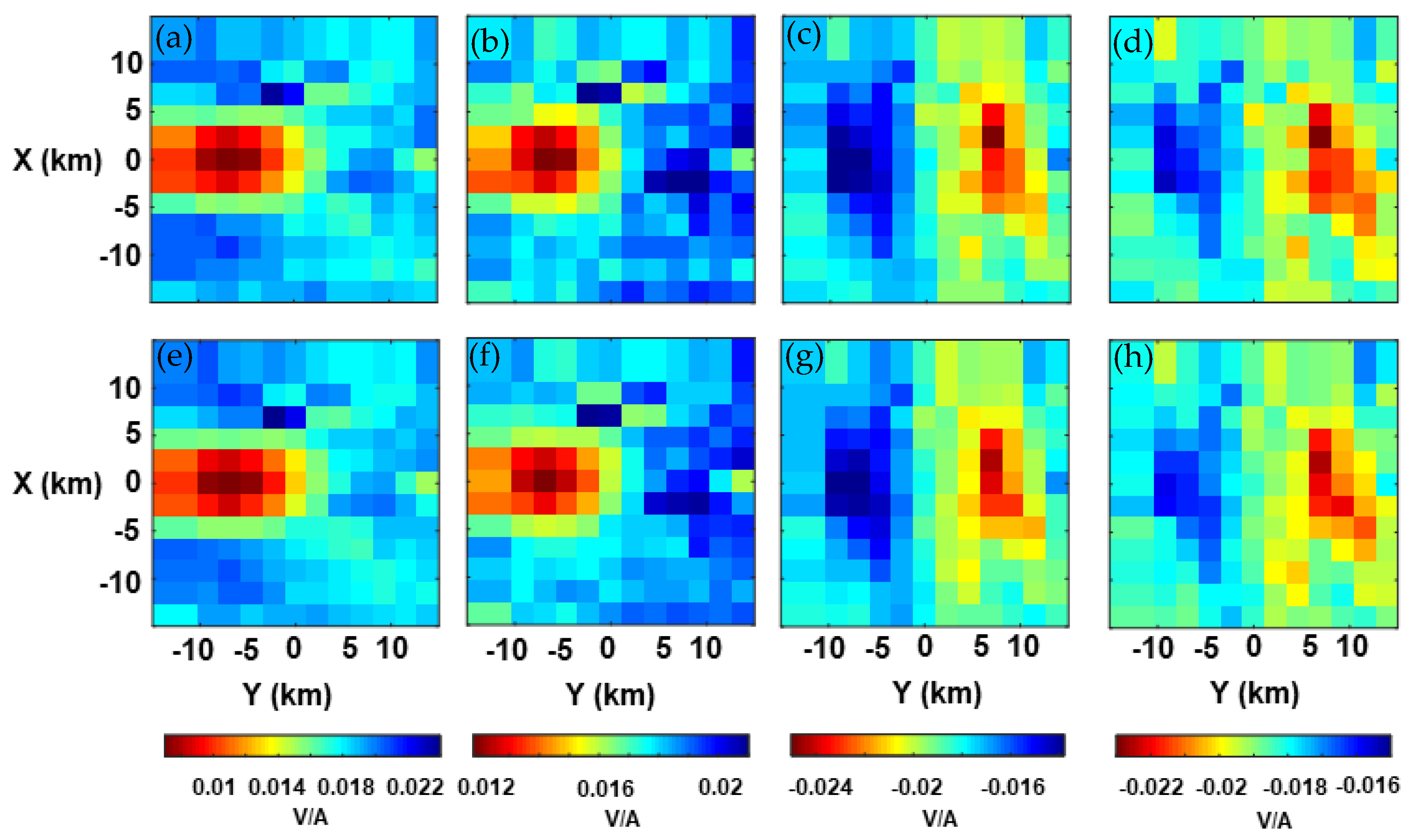
3.3. Isotropic and Anisotropic Blocks Model with Topography

To further test the performance of the developed algorithm, we design an isotropic and anisotropic blocks model, as shown in Figure 17. The background model is a homogeneous half-space with the resistivity of 300 $\mathsf{\Omega }\mathrm{m}$. The three principal resistivities of the anisotropic block are ${\rho }_x/{\rho }_y/{\rho }_z=10 \mathsf{\Omega }\mathrm{m}/100 \mathsf{\Omega }\mathrm{m}/10 \mathsf{\Omega }\mathrm{m}$, and its central location is (0, −7.5, 5.5) km. The resistivity of the isotropic block is $1000 \mathsf{\Omega }\mathrm{m}$, and its central location is (0, 7.5, 5.5) km. The full impedance tensor data for 12 frequencies, evenly spaced in the logarithmic scale from 0.01 Hz to 100 Hz, at 169 sites are used for inversion. We add 2% Gauss random noise to the synthetic data. The topography in the inversion domain is shown in Figure 18.

The whole simulation domain extends from −100 km to 100 km in the horizontal direction and from −20 km to 80 km in the vertical direction. The inversion domain extends from −20 km to 20 km in the horizontal direction and from −1.16 km to 20 km in the vertical direction. The mesh for forward modeling is discretized into 824,132 cells. The inversion domain is discretized into 200,934 cells, and the total number of cells for the inversion mesh is 644,824. The initial and reference models of the inversion are a homogeneous half-space with the resistivity of $100 \mathsf{\Omega }\mathrm{m}$. The standard error is set to $0.02·sqrt\left(\left|Z_{xy}·Z_{yx}\right|\right)$. The maximum number of inversion iterations is set to 10, and the threshold RMS for the inversion is 1.05.

The convergence plot is shown in Figure 19, we can see that the RMS decreases from 21.72 to 1.05 after five iterations, the runtime is 8.2 h and the memory consumption is 99.2 GB.

The inversion results are shown in Figure 20 and Figure 21, we can see that the shape and position of the isotropic and anisotropic blocks are well recovered. The inversion does not produce obvious artifacts for the isotropic anomalous body.

The data fitting is shown in Figure 22, we choose the Z_xy and Z_yx components at the frequency of 0.285 Hz as an example. We can see that the observed data compare well with the predicted data.

4. Conclusions

In this paper, we develop a triaxial anisotropic 3-D MT inversion algorithm with unstructured tetrahedral mesh. To reduce the memory requirement, we transform the algorithm from the model space to the data space and derived the inversion workflow using the Gauss–Newton approach. In the data-space inversion, the model update direction can be effectively solved by the parallel direct solver.

We compare the efficiency of the model-space and data-space methods by an example. We found that the data-space algorithm requires much less memory and computation time than the model space method when the number of model parameters is large. We demonstrate the effectiveness and applicability of the anisotropic inversion algorithm by several synthetic models. The electrical structures in the principal X and Y directions can be well recovered, but the resistivity of the principal Z direction cannot be reasonably recovered by the current inversion algorithm. We will apply the developed anisotropic inversion algorithm in data space to the field data in the future research.

References

1. Hübert, J.; Lee, B.M.; Liu, L.; Unsworth, M.J.; Richards, J.P.; Abbassi, B.; Cheng, L.; Oldenburg, D.W.; Legault, J.M.; Rebagliati, M. Three-dimensional imaging of a Ag-Au-rich epithermal system in British Columbia, Canada, using airborne z-axis tipper electromagnetic and ground-based magnetotelluric data. Geophysics 2016, 81, B1–B12. [Google Scholar] [CrossRef] [Green Version]
2. Wu, Y.; Han, J.; Liu, Y.; Liu, L.; Guo, L.; Guang, Y.; Zhang, Y.; Li, S. Three-dimensional electrical structures and mineralization significance in the Shuangjianzishan ore-concentrated area, Inner Mongolia. Chin. J. Geophys. 2021, 64, 1291–1304. (In Chinese) [Google Scholar]
3. Bai, D.; Unsworth, M.J.; Meju, M.A.; Ma, X.; Teng, J.; Kong, X.; Sun, Y.; Sun, J.; Wang, L.; Jiang, C.; et al. Crustal deformation of the eastern Tibetan plateau revealed by magnetotelluric imaging. Nat. Geosci. 2010, 3, 358–362. [Google Scholar] [CrossRef]
4. Ogawa, Y.; Ichiki, M.; Kanda, W.; Mishina, M.; Asamori, K. Three-dimensional magnetotelluric imaging of crustal fluids and seismicity around Naruko volcano, NE Japan. Earth Planets Space 2014, 66, 158. [Google Scholar] [CrossRef] [Green Version]
5. Yang, W.; Jin, S.; Zhang, L.; Qu, C.; Hu, X.; Wei, W.; Yu, C.; Yu, P. The three-dimensional resistivity structures of the lithosphere beneath the Qinghai-Tibet Plateau. Chin. J. Geophys. 2020, 63, 817–827. (In Chinese) [Google Scholar]
6. Piña-Varas, P.; Ledo, J.; Queralt, P.; Marcuello, A.; Bellmunt, F.; Hidalgo, R.; Messeiller, M. 3-D magnetotelluric exploration of Tenerife geothermal system (Canary Islands, Spain). Surv. Geophys. 2014, 35, 1045–1064. [Google Scholar] [CrossRef]
7. Zhang, C.; Hu, S.; Song, R.; Zuo, Y.; Jiang, G.; Lei, Y.; Zhang, S.; Wang, Z. Genesis of the hot dry rock geothermal resources in the Gonghe basin: Constraints from the radiogenic heat production rate of rocks. Chin. J. Geophys. 2020, 63, 2697–2709. (In Chinese) [Google Scholar]
8. Christensen, N.B. Difficulties in determining electrical anisotropy in subsurface investigations. Geophys. Prospect. 2000, 48, 1–19. [Google Scholar] [CrossRef]
9. Wannamaker, P.E. Anisotropy versus heterogeneity in continental solid Earth electromagnetic studies: Fundamental response characteristics and implications for physicochemical state. Surv. Geophys. 2005, 26, 733–765. [Google Scholar] [CrossRef]
10. Newman, G.A.; Commer, M.; Carazzone, J.J. Imaging CSEM data in the presence of electrical anisotropy. Geophysics 2010, 75, F51–F61. [Google Scholar] [CrossRef]
11. Guo, Z.; Wei, W.; Ye, G.; Jin, S.; Jing, J. Canonical decomposition of magnetotelluric responses: Experiment on 1D anisotropic structures. J. Appl. Geophys. 2015, 119, 79–88. [Google Scholar] [CrossRef]
12. Liu, Y.; Xu, Z.; Li, Y. Adaptive finite element modelling of three-dimensional magnetotelluric fields in general anisotropic media. J. Appl. Geophys. 2018, 151, 113–124. [Google Scholar] [CrossRef]
13. Weidelt, P. 3-D conductivity models: Implications of electrical anisotropy. In Three-Dimensional Electromagnetics; Society of Exploration Geophysicists: Houston, TX, USA, 1999. [Google Scholar]
14. Miensopust, M.P.; Jones, A.G. Artefacts of isotropic inversion applied to magnetotelluric data from an anisotropic Earth. Geophys. J. Int. 2011, 187, 677–689. [Google Scholar] [CrossRef]
15. Cao, H.; Wang, K.; Wang, T.; Hua, B. Three-dimensional magnetotelluric axial anisotropic forward modeling and inversion. J. Appl. Geophys. 2018, 153, 75–89. [Google Scholar] [CrossRef]
16. Li, Y.; Berlin, F.U.; Prag, J.P.; Brasse, H. Magnetotelluric inversion for 2D anisotropic conductivity structures Inversion methodology. In Kolloquium Elektromagnetische Tiefenforschung; Burg Ludwigstein; Deutsche Geophysikalische Gesellschaft e.V.: Königstein, Germany, 2003. [Google Scholar]
17. Pek, J.; Santos, F.; Li, Y. Non-linear conjugate gradient magnetotelluric inversion for 2-D anisotropic conductivities. In Proceedings of the 24 SchmuckerWeidelt-Colloquium, Neustadt an der Weinstraße, Germany, 19–23 September 2011. [Google Scholar]
18. Yu, G.; Farquharson, C.G.; Xiao, Q.; Li, M. Two-dimensional anisotropic magnetotelluric inversion using a limited-memory quasi-Newton method. Geophysics 2021, 87, E13–E34. [Google Scholar] [CrossRef]
19. Wang, K.; Wang, X.; Cao, H.; Lan, X.; Duan, C.; Luo, W.; Yuan, J. Magnetotelluric axial anisotropic parallelized 3D inversion based on cross gradient structural constraint. Chin. J. Geophys. 2021, 64, 1305–1319. (In Chinese) [Google Scholar]
20. Kong, W.; Tan, H.; Lin, C.; Unsworth, M.; Lee, B.; Peng, M.; Wang, M.; Tong, T. Three-dimensional inversion of magnetotelluric data for a resistivity model with arbitrary anisotropy. J. Geophys. Res. Solid Earth 2021, 126, e2020JB020562. [Google Scholar] [CrossRef]
21. Hauserer, M.; Junge, A. Electrical mantle anisotropy and crustal conductor: A 3-D conductivity model of the Rwenzori Region in western Uganda. Geophys. J. Int. 2011, 185, 1235–1242. [Google Scholar] [CrossRef] [Green Version]
22. Liu, Y.; Junge, A.; Yang, B.; Lower, A.; Cembrowski, M.; Xu, Y. Electrically anisotropic crust from three-dimensional magnetotelluric modeling in the western Junggar, NW China. J. Geophys. Res. Solid Earth 2019, 124, 9474–9494. [Google Scholar] [CrossRef] [Green Version]
23. Siripunvaraporn, W.; Egbert, G.; Lenbury, Y.; Uyeshima, M. Three-dimensional magnetotelluric inversion: Data-space method. Phys. Earth Planet. Inter. 2005, 150, 3–14. [Google Scholar] [CrossRef]
24. Hu, X.; Li, Y.; Yang, W.; Wei, W.; Guo, R.; Han, B.; Peng, R. Three-dimensional magnetotelluric parallel inversion algorithm using the data-space method. Chin. J. Geophys. 2013, 56, 484–493. (In Chinese) [Google Scholar]
25. Usui, Y.; Ogawa, Y.; Aizawa, K.; Kanda, W.; Hashimoto, T.; Koyama, T.; Yamaya, Y.; Kagiyama, T. Three-dimensional resistivity structure of Asama Volcano revealed by data-space magnetotelluric inversion using unstructured tetrahedral elements. Geophys. J. Int. 2016, 208, 1359–1372. [Google Scholar] [CrossRef]
26. Kordy, M.; Wannamaker, P.; Maris, V.; Cherkaev, E.; Hill, G. 3-dimensional magnetotelluric inversion including topography using deformed hexahedral edge finite elements and direct solvers parallelized on symmetric multiprocessor computers—Part II: Direct data-space inverse solution. Geophys. J. Int. 2016, 204, 94–110. [Google Scholar] [CrossRef] [Green Version]
27. Pek, J.; Santos, F.A.M. Magnetotelluric inversion for anisotropic conductivities in layered media. Phys. Earth Planet. Inter. 2006, 158, 139–158. [Google Scholar] [CrossRef]
28. Schenk, O.; Gärtner, K. Solving unsymmetric sparse systems of linear equations with PARDISO. Future Gener. Comput. Syst. 2004, 20, 475–487. [Google Scholar] [CrossRef]
29. Key, K. MARE2DEM: A 2-D inversion code for controlled-source electromagnetic and magnetotelluric data. Geophys. J. Int. 2016, 207, 571–588. [Google Scholar] [CrossRef]
30. Cai, H.; Long, Z.; Lin, W.; Li, J.; Lin, P.; Hu, X. 3D multinary inversion of controlled-source electromagnetic data based on the finite-element method with unstructured mesh. Geophysics 2021, 86, E77–E92. [Google Scholar] [CrossRef]
31. Wang, F.; Morten, J.P.; Spitzer, K. Anisotropic three-dimensional inversion of CSEM data using finite-element techniques on unstructured grids. Geophys. J. Int. 2018, 213, 1056–1072. [Google Scholar] [CrossRef]
32. Golob, G.H.; Loan, C.F.V. Matrix Computations, 4th ed.; Johns Hopkins University: Baltimore, MD, USA, 2013. [Google Scholar]
33. Pacheco, P.S. An Introduction to Parallel Programming; Morgan Kaufmann: Burlington, VT, USA, 2013. [Google Scholar]
34. Grayver, A.V.; Streich, R.; Ritter, O. Three-dimensional parallel distributed inversion of CSEM data using a direct forward solver. Geophys. J. Int. 2013, 193, 1432–1446. [Google Scholar] [CrossRef] [Green Version]
35. Usui, Y. 3-D inversion of magnetotelluric data using unstructured tetrahedral elements: Applicability to data affected by topography. Geophys. J. Int. 2015, 202, 828–849. [Google Scholar] [CrossRef] [Green Version]
36. Xiang, Y.; Yu, P.; Zhang, L.; Feng, S.; Utada, H. Regularized magnetotelluric inversion based on a minimum support gradient stabilizing functional. Earth Planets Space 2017, 69, 158. [Google Scholar] [CrossRef] [Green Version]
37. Cao, X.; Huang, X.; Yin, C.; Yan, L.; Zhang, B. 3D MT anisotropic inversion based on unstructured finite-element method. J. Environ. Eng. Geoph. 2021, 26, 49–60. [Google Scholar] [CrossRef]
38. Zhang, L.; Koyama, T.; Utada, H.; Yu, P.; Wang, J. A regularized three-dimensional magnetotelluric inversion with a minimum gradient support constraint. Geophys. J. Int. 2012, 189, 296–316. [Google Scholar] [CrossRef] [Green Version]
39. Menke, W.; Creel, R. Gaussian process regression reviewed in the context of inverse theory. Surv. Geophys. 2021, 42, 473–503. [Google Scholar] [CrossRef]
Figure 1. Workflow for 3-D magnetotelluric inversion with triaxial anisotropy.
Minerals 12 00734 g001
Figure 2. The performance of the model-space and the data-space inversion algorithms.
Minerals 12 00734 g002
Figure 3. Panels (a) and (b) show the SM3 model from Cao et al., 2018 at x = 0 km and z = 1 km, respectively. The black dots represent the MT receivers.
Minerals 12 00734 g003
Figure 4. Convergence plot for the SM3 model. The black dashed line indicates the threshold RMS.
Minerals 12 00734 g004
Figure 5. The inverted principal conductivity along the X-axis. Panels (a) and (b) show the true model and the recovered model at x = 0 km. Panels (c) and (d) show the true model and recovered model at y = 0 km. Panels (e) and (f) show the true model and the recovered model at z = 1 km.
Minerals 12 00734 g005
Figure 6. The inverted principal conductivity along the Y-axis. Panels (a) and (b) show the true model and recovered model at x = 0 km. Panels (c) and (d) show the true model and recovered model at y = 0 km. Panels (e) and (f) show the true model and the recovered model at z = 1 km.
Minerals 12 00734 g006
Figure 7. The inverted principal conductivity along Z-axis. Panels (a) and (b) show the true model and the recovered model at x = 0 km. Panels (c) and (d) show the true model and the recovered model at y = 0 km. Panels (e) and (f) show the true model and the recovered model at z = 1 km.
Minerals 12 00734 g007
Figure 8. The inverted anisotropic coefficient. Panels (a) and (b) show the true model and the recovered model at x = 0 km. Panels (c) and (d) show the true model and the recovered model at y = 0 km. Panels (e) and (f) show the true model and the recovered model at z = 1 km.
Minerals 12 00734 g008
Figure 9. Data fitting of Zxy and Zyx components at the frequency of 5 Hz. Panels (a) and (b) show the real and imaginary parts of the observed Zxy component. Panels (c) and (d) show the real and imaginary parts of the observed Zyx component. Panels (e) and (f) show the real and imaginary parts of the predicted Zxy component. Panels (g) and (h) show the real and imaginary parts of predicted Zyx component.
Minerals 12 00734 g009
Figure 10. Panels (a) and (b) show the true model at y = 0 km and z = 6 km. Panels (c) and (d) show the isotropic inversion results at y = 0 km and z = 6 km. The black dots represent MT receivers.
Minerals 12 00734 g010
Figure 11. Anisotropic inversion results at y = 0 km. Panels (a), (c), and (e) show the true model for the principal X, Y directions and the anisotropic coefficient. Panels (b), (d), and (f) show the corresponding inversion results.
Minerals 12 00734 g011
Figure 12. Anisotropic inversion results at z = 6 km. Panels (a), (c), and (e) show the true model for the principal X and Y directions, and the anisotropic coefficient. Panels (b), (d), and (f) show the corresponding inversion results.
Minerals 12 00734 g012
Figure 13. Convergence plot for the isotropic and anisotropic inversion. The black dashed line indicates the threshold RMS.
Minerals 12 00734 g013
Figure 14. Data fitting for Zxy and Zyx components at the frequency of 0.46 Hz. Panels (a) and (b) show the real and imaginary parts of observed Zxy component. Panels (c) and (d) show the real and imaginary parts of observed Zyx component. Panels (e) and (f) show the real and imaginary parts of predicted Zxy component for isotropic inversion. Panels (g) and (h) show the real and imaginary parts of predicted Zyx component for isotropic inversion. Panels (i) and (j) show the real and imaginary parts of predicted Zxy component for anisotropic inversion. Panels (k) and (l) show the real and imaginary parts of predicted Zyx component for anisotropic inversion.
Minerals 12 00734 g014
Figure 15. Anisotropic inversion results at y = 0 km. Panels (a) and (b) show the inverted resistivity in the principal X direction when including and excluding the vertical resistivity in the inversion. Panels (c) and (d) show the inverted resistivity in the principal Y direction when including and excluding the vertical resistivity in the inversion. Panels (e) and (f) show the inverted anisotropic coefficient when including and excluding the vertical resistivity in the inversion.
Minerals 12 00734 g015
Figure 16. Anisotropic inversion results at z = 6 km. Panels (a) and (b) show the inverted resistivity in the principal X direction when including and excluding the vertical resistivity in the inversion. Panels (c) and (d) show the inverted resistivity in the principal Y direction when including and excluding the vertical resistivity in the inversion. Panels (e) and (f) show the inverted anisotropic coefficient when including and excluding the vertical resistivity in the inversion.
Minerals 12 00734 g016
Figure 17. Panels (a) and (b) show the isotropic and anisotropic blocks model at x = 0 km and z = 6 km, respectively. The black dots represent the MT receivers.
Minerals 12 00734 g017
Figure 18. The topography in the inversion domain (with exaggeration in the vertical direction). The black dots indicate the MT receivers.
Minerals 12 00734 g018
Figure 19. Convergence plot for the isotropic and anisotropic blocks model with topography. The black dashed line indicates the threshold RMS.
Minerals 12 00734 g019
Figure 20. Anisotropic inversion results at x = 0 km. Panels (a), (c), and (e) show the true model for principal X and Y directions, and the anisotropic coefficient. Panels (b), (d), and (f) show the anisotropic inversion results for the principal X and Y directions, and the anisotropic coefficient.
Minerals 12 00734 g020
Figure 21. Anisotropic inversion results at z = 5.5 km. Panels (a), (c), and (e) show the true model for the principal X and Y directions, and the anisotropic coefficient. Panels (b), (d), and (f) show the anisotropic inversion results for the principal X and Y directions, and the anisotropic coefficient.
Minerals 12 00734 g021
Figure 22. Data fitting for Zxy and Zyx components at the frequency of 0.285 Hz. Panels (a) and (b) show the real and imaginary parts of observed Zxy component. Panels (c) and (d) show the real and imaginary parts of the observed Zyx component. Panels (e) and (f) show the real and imaginary parts of the predicted Zxy component. Panels (g) and (h) show the real and imaginary parts of the predicted Zyx component.
Minerals 12 00734 g022
Publisher’s Note: MDPI stays neutral with regard to jurisdictional claims in published maps and institutional affiliations.