Abstract
The magnetotelluric (MT) method is widely applied in petroleum, mining, and deep Earth structure exploration but suffers from cultural noise. This noise will distort apparent resistivity and phase, leading to false geological interpretation. Therefore, denoising is indispensable for MT signal processing. The sparse representation method acts as a critical role in MT denoising. However, this method depends on the sparse assumption leading to inadequate denoising results in some cases. We propose an alternative MT denoising approach, which can achieve accurate denoising without assumptions on datasets. We first design a residual network (ResNet), which has an excellent fitting ability owing to its deep architecture. In addition, the ResNet network contains skip-connection blocks to guarantee the robustness of network degradation. As for the number of training, validation, and test datasets, we use 10,000,000; 10,000; and 100 field data, respectively, and apply the gradual shrinkage learning rate to ensure the ResNet’s generalization. In the noise identification stage, we use a small-time window to scan the MT time series, after which the gramian angular field (GAF) is applied to help identify noise and divide the MT time series into noise-free and noise data. We keep the noise-free data section in the denoising stage, and the noise data section is fed into our network. In our experiments, we test the performances of different time window sizes for noise identification and suppression and record corresponding time consumption. Then, we compare our approach with sparse representation methods. Testing results show that our approach can obtain the desired denoising results. The accuracy and loss curves show that our approach can well suppress the MT noise, and our network has a good generalization. To further validate our approach’s effectiveness, we show the apparent resistivity, phase, and polarization direction of test datasets. Our approach can adjust the distortion of apparent resistivity and phase and randomize the polarization direction distribution. Although our approach requires the high quality of the training dataset, it achieves accurate MT denoising after training and can be meaningful in cases of a severe MT noisy environment.
1. Introduction
The magnetotelluric method is a crucial geophysical exploration technique that uses natural current sources to detect underground targets. When the electromagnetic wave is propagating underneath the ground, the induced charges and currents appear at different depths, as different frequencies of electromagnetic waves have different skin depths. By analyzing the measured electromagnetic fields on the air–Earth interface, we can infer the conductivity distributions of underground structures [1,2,3,4,5].
The MT method is based on the assumption of plane wave source [6,7,8,9]. On the ground, we measure time series of two horizontal components of electric responses, in the x-direction and in the y-direction. We also can measure time series of three components of magnetic responses, in the x-direction, in the y-direction and in the z-direction in the time domain. The x axis is perpendicular to y on Earth’s surface. The Fourier transformations of these time series (which are , , , , and ) have the following linear relationship [10,11]:
where is impedance tensor, and are tippers. We use and its real part and imaginary part to compute the apparent resistivity and phase :
where and denote the angular frequency and magnetic permeability of free space, respectively. We then use the apparent resistivity and phase to infer the underground structure.
However, the MT data are inevitably corrupted by cultural noise when we collect them in the area with electromagnetic noises, such as near cities. In order to remove noise, there have been substantial denoising methods proposed in recent years. They can be divided into five classes such as the remote reference method [12,13], the robust estimation method [14,15], the data section selection technique [16,17], the inversion rectification method [18,19], and the time–frequency domain suppression method [20,21].
The remote reference method is a widely used technique for MT denoising. Gamble et al. [22] collected MT data from two sites, which were far away from each other, and set one site as the remote reference site. They used the irrelevance of noise between the remote and local sites to achieve MT noise removal. Ritter et al. [23] proposed that the magnetic field’s correlations between the remote and local sites acted as a pivotal role in MT denoising. However, the performance of this denoising method depends on the quality of the selected remote reference site. As for the robust estimation technique, Sims et al. [24] used the self and cross power spectrums to estimate the impedance tensor. Sutarno et al. [25] presented the robust M-estimation method. Chave [26] combined the maximum likelihood estimator with robust estimation to obtain a good MT response. The robust estimation relies on the proportion of useful MT data. When MT data are interfered by long-period noise, this method does not work well. In this case, the data section selection does not perform well either. However, when MT data only contain short-period noise, this method can obtain good apparent resistivity. Escalas et al. [27] selected appropriate sizes of time series and utilized their wavelet coefficients to suppress cultural noise successfully. Furthermore, many geophysicists attenuate the MT noise in apparent resistivity and phase rather than the time series. Because this kind of method rectifies apparent resistivity and phase via MT inversion, it requires the majority of points of apparent resistivity and phase keeping correct. Parker et al. [28] rectified the distortion of apparent resistivity via one-dimensional (1D) MT inversion. Guo et al. [29] applied the nonlinear Bayesian formulation to analyze the MT noise influence and concluded that the parameter’s uncertainties were underestimated when using diagonal covariance. Time–frequency domain suppression is also an effective way to attenuate MT noise. Concerning the time domain suppression, Tang et al. [30] used mathematical morphology filtering to remove the intense natural noise from MT data. However, this method caused the loss of low frequency and could not deal with impulse noise. In frequency domain suppression, Carbonari et al. [31] combined the wavelet transformation with polarization direction analysis to attenuate the MT noise. This method was effective in both synthetic and field MT data. Ling et al. [32] used the varying thresholds in wavelet coefficients to suppress MT noise, outperforming the fixed thresholds for wavelet coefficients in MT denoising. However, the wavelet transformation cannot remove the MT noise well in some cases because its base is fixed while the MT signal is complex. Only using one fixed base is hard to represent the various MT signals well. Thus, Li et al. [33] presented a learning-based MT denoising method to solve this problem. This method can use some optimization algorithms to update the base. Thus, it can change the base according to the signal itself, which contributes to more accurate apparent resistivity than the wavelet transformation. Nevertheless, this method is still based on the assumption of sparse representation. When we collect the MT data in a complex environment, the learning base still cannot represent the MT data well.
Recently, deep learning has made breakthroughs, and it has brought reform in many fields, including geophysics [34]. The neural network, which belongs to deep learning methods, contains many layers regarded as the mapping function. When we use some optimization algorithms to train the neural network, it can find the mapping relationship between the samples and labels. That is to say, we can find the noise-free and noise data mapping relationship by a neural network. Unlike the sparse representation methods, deep learning is not based on any signal sparse assumptions. Thus, it can achieve better denoising performance than sparse representation methods [35]. Carbonari et al. [36] combined the self-organizing map neural networks with data section selection to complete the MT cultural noise removal. It achieves more accurate denoising results than some convention MT denoising methods. However, this method is complicated and overloaded. Chen et al. [37] applied the recurrent neural network to suppress the MT noise. This method meets the feature of the MT time series since it has the memory cells, which can save the weights and not damage the structure of the time series. Nevertheless, it has shortages such as long-term dependencies and vanishing gradient problems.
Inspired by the good fitting ability of deep learning, we design a deep residual network (ResNet) in this paper. Similar to other deep learning methods, our network needs a high-quality training dataset to achieve accurate MT denoising. To fulfill this requirement, we use 100,000,000; 10,000; and 100 samples for training, validation, and test datasets, respectively. All of the training, validation, and test datasets are the field data to make our experiments realistic. In the training and validation datasets, the additive noise is extracted from field data. We set a variable learning rate that gradually shrinks to improve the network’s generalization. To keep the noise-free data from being corrupted during denoising, we segregate our denoising flow into two parts, called noise identification and suppression, respectively. The time window is applied to shrink the MT data size and to facilitate training. We also compare the influences of different window sizes for MT noise identification and suppression. Furthermore, the gramian angular field (GAF) is applied to help identify the noise. At the end of our experiments, we use our approach to deal with the test datasets, whose noise level is unknown.
The rest of the paper is organized as follows. In the first section, the computation and architecture of the ResNet, which is used in our study, is discussed, followed by a brief introduction of our whole denoising flow. In the next section, before we show the noise identification examples, the basic theory of the GAF is introduced. We also test the influences of different window sizes for identification accuracy in this section. In the section to follow, we compare our approach with some sparse representation methods, and we test the performances of different window sizes for denoising. To evaluate the test dataset denoising performances, we use the apparent resistivity and phase and polarization direction to show our approach’s good generalization. Finally, according to our above studies and discussions, we draw some conclusions.
2. ResNet
2.1. Basics Calculations for ResNet
This paper uses the ResNet to suppress MT noise since it is robust for network degradation. Similar to other neural networks, the ResNet can find the mapping relationship between samples and labels, which are the noise and noise-free MT data in this paper, respectively. The MT data with cultural noise can be defined as follows:
where , , and denote noise MT data, noise-free MT data, and cultural noise, respectively. In the case of sufficient training datasets, the ResNet can learn the mapping relationship between the samples and labels via updating the parameters of neural network , which contains weight value and bias value . Let and represent the -th label and prediction of the ResNet with training datasets. The L2 norm can be used to optimize the , and the objective function of training ResNet can be represented as [38]:
Equation (4) can be solved by some optimization algorithms such as the ADAM algorithm [39].
2.2. The Architecture of the ResNet
Usually, after surpassing a certain number of layers, the neural network’s fitting ability will decrease as its architecture becomes deep. However, the ResNet contains skip-connection blocks that can transmit the information from shallow layers to deep layers directly and avert information loss [40,41,42]. The skip-connection block in our study is shown in Figure 1. According to the output size, we can divide the skip-connection block into two classes, such as the identity block (Figure 1a) and the convolution block (Figure 1b). In the identity block, we have the relationship between input and output as follows:
where denotes the function of these below two layers in Figure 1a, is the rectified linear unit. In Equation (5), can acquire the information of directly by adding. Similarly, in the convolution block, we can rewrite Equation (5) as:
where is the function of this above layer in Figure 1b. Furthermore, the size of the convolution kernel in is 1. Thus, only changes the channels (e.g., the stride in this block is set to 2, which results in different sizes between the input and output of this block) and does not influence the value of . That is to say, can still acquire the information of from . We use these two kinds of skip-connection blocks to build our ResNet. Here, we take the input with a length of 32 as an example. When in the noise suppression, the architecture of the ResNet can be displayed in Figure 2.
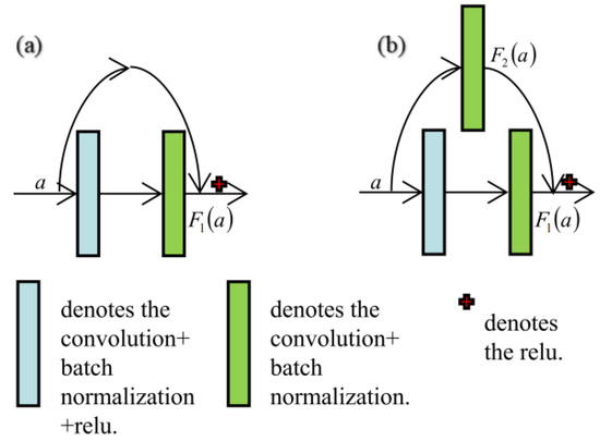
Figure 1.
Skip-connection block in the ResNet: (a) identity block; (b) convolution block.
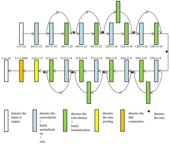
Figure 2.
The architecture of the ResNet for MT noise identification and suppression.
Nevertheless, in noise identification, the sizes of all inputs and outputs will change in Figure 2. Owing to the GAF’s expansion function, the shape of input will become 32 × 32 rather than 1 × 32. Thus, the second dimensions of all inputs and outputs for convolutional and pooling layers in Figure 2 will be the same as their third dimensions (i.e., they are no longer 1). Meanwhile, the input size in full connection is 1 × 1 × 8192 instead of 1 × 1 × 2048, and the output size in this layer is 1 × 1 × 2 instead of 1 × 1 × 32.
About the parameters in this ResNet, all the kernel sizes are 3 except the convolution blocks, whose kernel sizes are kept constant 1. The padding of 1 is applied in all convolutional and pooling layers except the convolution blocks. Furthermore, the strides are set to 2 in the sixth, tenth, and fourteenth convolutional layers and all convolution blocks, while the others are set to 1. To facilitate potential readers who want to repeat our study and make a comparison with their research, we show our computer environment as follows:
- CPU: Intel i9 12900K, 5.20 GHz, 16x (Key Laboratory of Metallogenic Prediction of Nonferrous Metals and Geological Environment Monitoring, Central South University, Changsha, China)
- GPU: Nvidia GeForce GTX 3090, 24 GB
In addition, we build and train this ResNet on Pytorch [43].
Figure 3 shows the workflow diagram of our study. First, we use the time window to scan the MT time series and obtain the MT data section. Second, the GAF is applied to expand the 1D data section (i.e., one channel MT time series section) to 2D and help identify. Third, the ResNet is used for noise identification and suppression.
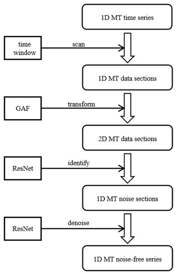
Figure 3.
The whole workflow of our study.
3. MT Noise Identification
3.1. Gramian Angular Field
After completing the ResNet building, we use the time window to cut the MT time series and obtain the data section. Then, the Gramian angular summation field (GASF) or the gramian angular difference field (GADF) is applied to this data section since this method can expand the 1D data section to 2D and can help identify. Wang et al. [44] proposed the GAF of time series for identification in the CNN, and they found that this technique could reduce mean-square error. Hong et al. [45] applied the GAF in the CNN cascaded with the long short-term memory against overfitting. Thanaraj et al. [46] tested the performances of different neural networks by the GAF, and they showed that the GAF could improve the accuracy of electroencephalogram identification. When we use the GAF, we should normalize the data section within the [−1, 1] range to meet the independent variable of polar coordinate [47]:
where and are the data section and its normalization in time point , respectively. is the maximum of the absolute value of . In this case, we transform it into the polar coordinate and have the relationship as follows:
where is the polar coordinate corresponding to . Hence, the GASF for and can be defined by:
Similarly, when we use the GADF, we can rewrite Equation (9) as follows:
Figure 4 shows shapes of the MT noise-free data and common MT noise such as harmonic, square, triangle, impulse, and step noise in the Cartesian coordinate, the polar coordinate, and the GAF. It is clear that the GAF can generate different kinds of 2D images according to different 1D MT noise. When the samples of 1D MT data are being acquired from left to right along the time axis, these samples are moving from top-left to bottom-right in the GAF at the same time. Thereby the GAF does not corrupt the sequence in time series, and its expansion in dimension helps identify MT noise.
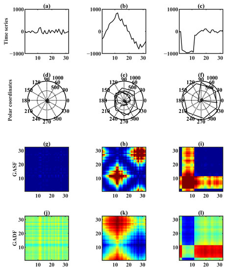
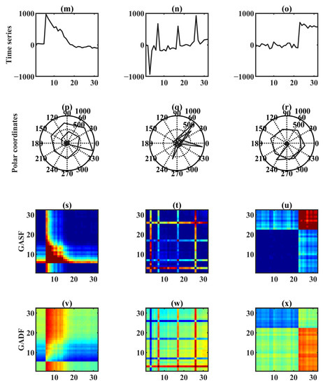
Figure 4.
The shapes of MT noise-free data and harmonic, square, triangle, impulse and step noises in different coordinates. (a–c) and (m–o) in the Cartesian coordinate. (d–f) and (p–r) in the polar coordinate. (g–i) and (s–u) in the GASF. (j–l) and (v–x) in the GADF. Red to Blue: It represents the amplitude is from large to small.
3.2. Training the ResNet for Identification
There are a number of 10,010,100 datasets in total, which contain 10,000,000 training datasets, 10,000 validation datasets, and 100 test datasets, and all three are field MT time series. These field data are collected in Qaidam basin, Qinghai province, China. The instrument and software for these field data acquisitions and apparent resistivity and phase computations are V5-2000 and SSMT-2000, respectively. In order to decrease the memory of computation, the time window is applied. Each MT time series in training and validation datasets will be cut randomly to obtain the same number of datasets. As for the training datasets, the labels are 10,000,000 noise-free data, while every 2,000,000 of them are corrupted by the harmonic, square, triangle, impulse, and step noises, respectively, to form samples, which are both extracted from other sources field MT data. Similarly, in the validation datasets, 10,000 of them are noise-free to form labels, while every 2000 of them are corrupted by harmonic, square, triangle, impulse, and step noises, respectively, to form samples. The noise level of test datasets is unknown. This dataset format is used for the suppression stage, but it is a little different in the identification stage since we should change the labels to meet the classification problem. Before training the ResNet for identification, we manually mark the training and validation datasets as noise-free or noise data. Thus, the samples are the noise-free or noise sections that are cut by windows while the labels are 0 and 1. The number 0 represents those data sections without noise, while 1 represents those data sections with noise. In the identification stage, the loss function is Cross-Entropy loss. After GAF transformation, we feed these GAF images into our neural network and begin to train. As for the optimizer, we use the Adam optimizer since this algorithm can keep the denominators from zeros. Furthermore, the validation datasets are used for hyper-parameters tuning. The outputs of the ResNet for identification are 0 and 1.
By checking 0 and 1 in the outputs and comparing them with training and validation datasets, we can count the accuracy and know the performance of the ResNet to detect noise. We also test the identification accuracy of different window sizes with 32 × 32, 64 × 64, 128 × 128, and 256 × 256 in the validation datasets. Moreover, their statistics are shown in Table 1. Table 2 shows the computational time of these window sizes in training. Thus, the different window sizes and GAF transformations hardly influence the identification accuracy in our ResNet. In addition, as the window size increases, the training time of the ResNet becomes longer. To reduce the computational memory as well as computational time, we choose a window size of 32 × 32 for the following MT noise identification. Figure 5 shows the loss and accuracy of identification, with a min-batch size of 100, a drop out of 0.5 in full connection, and an initial learning rate of 0.000005, which will be 0.9 smaller after every 5 epochs. As can be seen from Figure 5a, the loss decreases as the epoch increases. After 9 epochs, the loss curves of training and validation datasets become stable. In Figure 5b, the accuracy of identification is proportional to the epoch. Similarly, after 9 epochs, the accuracy curves in training and validation datasets also become stable. Thus, our ResNet has a good generalization in MT noise identification.

Table 1.
The identification accuracy of validation datasets with different window sizes.
Table 2.
The computational time of training with different window sizes.
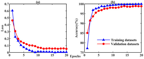
Figure 5.
The loss and accuracy of the ResNet for MT noise identification. (a) Loss curves and (b) accuracy curves of training and validation datasets.
3.3. The Identification of Test Datasets
Figure 6 and Figure 7 show the fifth and the twelfth test datasets. To see the MT noise identification via our ResNet clearly, we amplify some sections, where they are in the range from 10,001 to 12,000 sample points in the fifth test datasets, marked by the arrow in Figure 6. Figure 8 is the corresponding amplified sections in 6. Moreover, the data sections, which are identified as noise via our ResNet, are marked by red color. In Figure 8, the , , , and time series in the fifth test dataset contain severe impulse and triangle noise, and our ResNet can identify this kind of noise. Thus, our ResNet has a good performance in the identification of these noises. Thus, the step of MT noise identification is beneficial for the following MT noise suppression since we can conserve the noise-free data section.
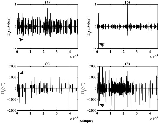
Figure 6.
The 5th test dataset. (a) , (b) , (c) , and (d) time series.
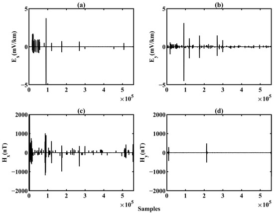
Figure 7.
The 12th test dataset. (a) , (b) , (c) , and (d) time series.
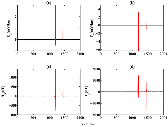
Figure 8.
The amplified sections in the 5th test dataset. MT noise identification of (a) , (b) , (c) , and (d) time series.
4. MT Noise Suppression
4.1. Training the ResNet for Denoising
After identification, we can know which data sections contain noise. In the suppression stage, it is the regression problem; thus, the loss function is the mean squared error loss, which Adam can solve. The samples are the MT data sections that are cut by windows and corrupted by the artificial noise, while the labels are the noise-free MT data sections. We restart training the ResNet to attenuate the identified MT noise, with a min-batch size of 100, a drop out of 0.5 in full connection, and an initial learning rate of 0.0001 will be 0.9 smaller after every five epochs. Once the ResNet completes training, those data sections that are identified as containing noise in the identification stage are fed into this ResNet. The outputs of the ResNet for suppression are the denoising MT data. Similarly, we use the time window to facilitate training, and the loss and computational time of different window sizes in our ResNet training are shown in Table 3. As we can see in Table 3, as the window size grows, the ResNet’s training becomes more time-consuming. Furthermore, the loss is nearly equivalent when the window sizes are 1 × 64, 1 × 128, and 1 × 256, which are both smaller than that of 1 × 32. Hence, we choose the window size of 1 × 64 to balance the loss and running time of the ResNet. Figure 9 shows the loss of training and validation datasets for MT noise suppression, which both descend gradually when epoch ascends. After about 75 epochs, both of these two loss curves are stable, proving the excellent generalization of our ResNet. To further validate our approach, we introduce the signal-to-noise ratio (SNR) as follows:
where denotes the denoising MT data. We compare our approach with the wavelet transformation [48], the dictionary learning [49], and the ResNet denoising without identification. Since then, we compute the average of denoising SNR for all validation datasets, listed in Table 4, and our approach obtains the highest SNR among these methods. Furthermore, we show a denoising sample of validation datasets in Figure 10. In Figure 10, the wavelet transformation cannot perform well because the denoising result contains considerable noise in the 30th and 50th points, while the denoising result of the dictionary learning allows a little noise in these two points to remain. Compared with the wavelet transformation and the dictionary learning, the ResNet’s denoising results are better and nearly remove all noise. The ResNet, which combines the denoising with identification, can better retain the noise-free data section than that without identification. Therefore, our approach has the best MT denoising performance among these MT denoising methods.
Table 3.
The validation dataset loss and the training running time with different window sizes.
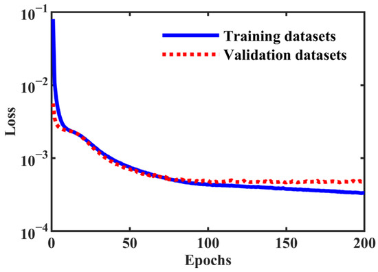
Figure 9.
The loss of the ResNet for MT noise suppression.
Table 4.
The average denoising SNR of all validation datasets for different methods.
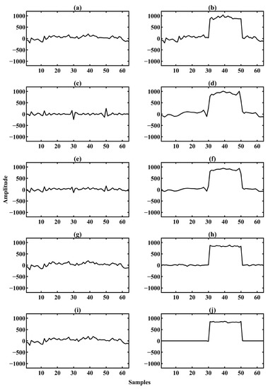
Figure 10.
A denoising sample in validation datasets. (a) Noise-free and (b) Noise data. The denoising results of (c) the wavelet, (e) the dictionary learning, (g) the ResNet without identification and (i) our approach. The difference between the denoising results of (d) the wavelet, (f) the dictionary learning, (h) the ResNet without identification and (j) our approach with noise data.
4.2. The Denoising of Test Datasets
We use this trained neural network to process all test datasets and show the denoising results of the fifth test dataset in Figure 11, while we show those of the twelfth test dataset in Figure 12. The denoising results of the corresponding amplified section in Figure 6 are shown in Figure 13. From these figures, we can see that the identified noise is both attenuated, and the noise-free data sections are well protected simultaneously. When we deal with the test datasets, the apparent resistivity, phase, and polarization direction can be regarded as the norm of MT denoising performance [50]. We continue to take the fifth and twelfth test datasets as examples. Figure 14 and Figure 15 show their apparent resistivity and phase curves before and after denoising via our approach. Figure 16 and Figure 17 show their polarization directions. In Figure 14 and Figure 15, as for the noise data, the apparent resistivity curves are smooth and continuous in the high frequency, while they are in a state of chaos and distortion in the low frequency. After denoising by our approach, the apparent resistivity curves become smooth and continuous without chaos and distortion in the low frequency. These phenomena can also be seen in the phase curves. The noise data phase is diffuse while the denoising data phase stays coherent in the low frequency. Therefore, the proposed approach is effective for the field MT data denoising since it can rectify the distortions in apparent resistivity and phase.
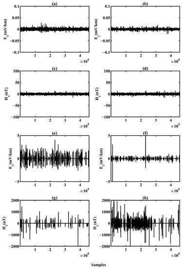
Figure 11.
The denoising results of the 5th test dataset. (a–d) are the denoising results for , , , and , respectively. (e–h) are the extracted noise for , , , and , respectively.
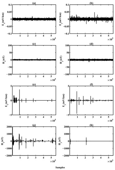
Figure 12.
The denoising results of the 12th test dataset. (a–d) are the denoising results for , , , and , respectively. (e–h) are the extracted noise for , , , and , respectively.
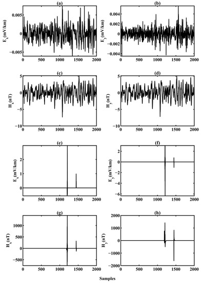
Figure 13.
The denoising results of amplified section in the 5th test dataset. (a–d) are the denoising results for , , , and , respectively. (e–h) are the extracted noise for , , , and , respectively.
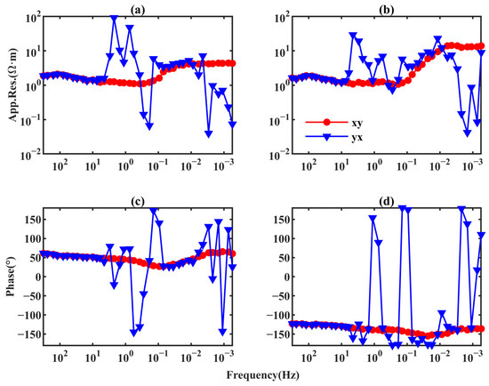
Figure 14.
The apparent resistivity and phase of the 5th test dataset. (a) , (b) , (c) and (d) curves.
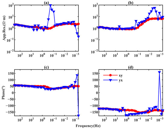
Figure 15.
The apparent resistivity and phase of the 12th test dataset. (a) , (b) , (c) and (d) curves.
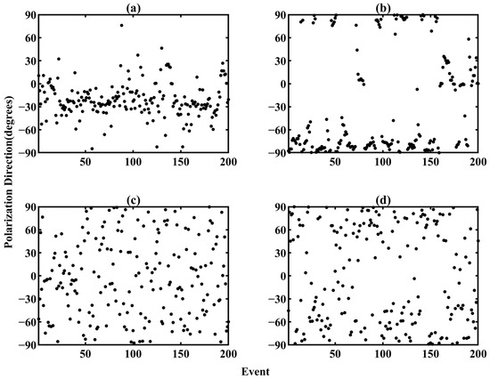
Figure 16.
The polarization direction of the 5th test dataset. The electric field of (a) noise data and (c) denoising data at 0.2 Hz. The magnetic field of (b) noise data and (d) denoising data at 0.2 Hz. Dots denote the polarization direction of different data sections.
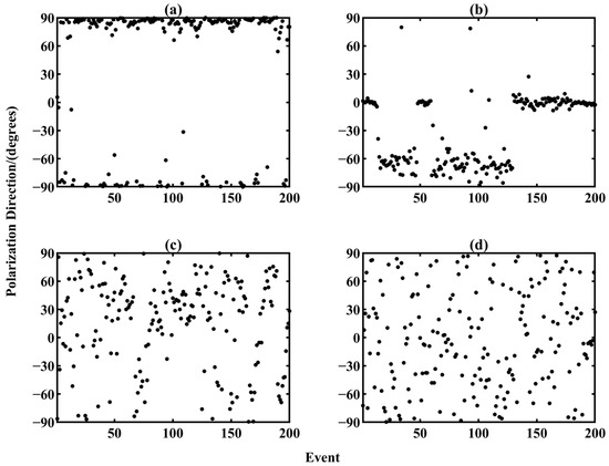
Figure 17.
The polarization direction of the 12th test dataset. The electric field of (a) noise data and (c) denoising data at 0.2 Hz. The magnetic field of (b) noise data and (d) denoising data at 0.2 Hz. Dots denote the polarization direction of different data sections.
We compare our approach’s noise data and denoising results in Figure 16 and Figure 17 for polarization direction. From these two figures, we can see that the noise leads to points converging at some angles, such as the range from −60° to 0° and from −60° to −90° in Figure 16a,b, respectively, the range from −75° to −90° and from 75° to 90° in Figure 17a, and the range from −75° to −90° in Figure 17b. However, as for the denoising data, their polarization directions become overall random in electric and magnetic fields in Figure 16 and Figure 17. Therefore, these results support our approach to attenuate the MT noise well, even if this noise level is unknown for our ResNet.
5. Conclusions
In this paper, we propose a novel MT denoising approach. Based on deep learning, we design a deep neural network containing the skip-connection blocks to form the ResNet. Owing to the ResNet’s unique architecture, our network has an excellent fitting ability and robustness against network degradation. Furthermore, over 10,000,000 datasets and the variable learning rate are used in our network training to ensure the ResNet’s generalization. Our workflow is divided into two parts in terms of MT noise characteristics, called identification and suppression. Before training the ResNet, a time window is used to reduce computational memory. In the identification, the GAF is applied to expand the datasets’ space, which helps MT noise identification. After identification, we retain the noise-free data section and feed the noise data section into our network to achieve the MT noise suppression.
Our experiments show that our ResNet’s accuracy in the MT noise identification is relatively high at over 98%, which is beneficial for protecting the noise-free data section. In addition, our ResNet has a good generalization in identification. When the noise level is unknown, our ResNet can still identify it. Our tests also indicate whether the GASF or GADF does not influence the performance of MT noise identification. Similarly, the time window size does not influence the performance of identification, while its size is proportional to the running time of the ResNet.
As for the MT noise suppression, our experiments show that our approach has a state-of-the-art performance among sparse representation methods. We also find that with the expansion of time window size, the ResNet loss becomes smaller for the MT noise suppression, while this loss becomes stable after the time window size outweighs 1 × 64. Similar to the MT noise identification, as the time window size grows, the ResNet’s running time increases. In addition, our ResNet has good generalization. It can remove the noise whose level is unknown. Our approach can rectify the distortion of the apparent resistivity and phase and randomize the electric and magnetic fields’ polarization direction. Therefore, our approach can be useful in MT denoising, even if MT data suffer from harsh noises. Our approach can also be applied in other fields since it is not based on any signals’ assumptions. For example, our approach’s identification function can be applied in face recognition, electroencephalogram signal identification, machine fault diagnosis, etc. Simultaneously, its denoising function can be used in seismic deblending, image denoising, speech denoising, etc.
Although our approach has many good effects on MT denoising, it is not perfect for achieving denoising thoroughly. First, we should make a good training dataset to ensure the effectiveness of our network. In the MT noise identification, because our approach cannot obtain 100% accuracy, it allows a little noise to remain that will not be fed into our ResNet to denoise. When our ResNet meets the harmonic wave noise, its long period brings about our approach’s degradation, which will become the ResNet without identification. Since this noise is throughout the whole MT data, the identification function of our network is useless. In this paper, we only discuss the time window influences with the length ranging from 32 to 256 for our ResNet. Thus, expanding the time window out of this range and discussing these time windows’ influences are directions to improve our approach. In addition, training the apparent resistivity rather than the time series is a potential direction, which can overcome our approach’s degradation caused by harmonic wave noise.
Author Contributions
L.Z.: Conceptualization, Methodology, Software, Visualization, Investigation, Formal Analysis, Writing—Original Draft; Z.R.: Conceptualization, Software, Validation, Funding Acquisition, Resources, Supervision, Writing—Review and Editing; X.X.: Funding Acquisition, Resources, Supervision, Conceptualization, Data Curation, Writing—Review and Editing; J.T.: Funding Acquisition, Resources, Supervision, Writing—Review and Editing; G.L.: Software, Visualization, Resources, Supervision, Writing—Review and Editing. All authors have read and agreed to the published version of the manuscript.
Funding
This research was funded by the National Natural Science Foundation of China (41830107 and 41904076), the Shenzhen Science and Technology Program (JCYJ20210324125601005), the Innovation-Driven Project of Central South University (2021zzts0257), the Open Fund from Key Laboratory of Metallogenic Prediction of Nonferrous Metals and Geological Environment Monitoring, Ministry of Education (2021YSJS02), and the National Key R&D Program of China (2018YFC0603202).
Data Availability Statement
Data associated with this research are available and can be obtained by contacting the corresponding author.
Conflicts of Interest
The authors declare no conflict of interest.
References
- Vozoff, K. The magnetotelluric method. In Electromagnetic Methods in Applied Geophysics; Nabighian, M.N., Ed.; Society of Exploration Geophysicists: Tulsa, OK, USA, 1991; pp. 641–711. [Google Scholar]
- Simpson, F.; Bahr, K. Practical Magnetotellurics; Cambridge University Press: Cambridge, UK, 2005. [Google Scholar]
- Cai, J.; Tang, J.; Hua, X.; Gong, Y. An analysis method for magnetotelluric data based on the Hilbert–Huang Transform. Explor. Geophys. 2009, 40, 197–205. [Google Scholar] [CrossRef]
- Tong, X.Z.; Liu, J.X.; Xie, W.; Xu, L.H.; Guo, R.W.; Cheng, Y.T. Three-dimensional forward modeling for magnetotelluric sounding by finite element method. J. Cent. South Univ. Technol. 2009, 16, 136–142. [Google Scholar] [CrossRef]
- Tang, J.T.; Wang, F.Y.; Ren, Z.Y.; Guo, R.W. 3-D direct current resistivity forward modeling by adaptive multigrid finite element method. J. Cent. South Univ. Technol. 2010, 17, 587–592. [Google Scholar] [CrossRef]
- Tikhonov, A.N. On determining electrical characteristics of the deep layers of the Earth’s crus. Dokl. Akad. Nauk. 1950, 73, 295–297. [Google Scholar]
- Cagniard, L. Basic theory of the magnetotelluric method of geophysical prospecting. Geophysics 1953, 18, 605–635. [Google Scholar] [CrossRef]
- Chave, A.D.; Jones, A.G. The Magnetotelluric Method. Theory and Practice; Cambridge University Press: Cambridge, UK, 2012. [Google Scholar]
- Wang, H.; Liu, W.; Xi, Z.Z.; Fang, J.H. Nonlinear inversion for magnetotelluric sounding based on deep belief network. J. Cent. South Univ. 2019, 26, 2482–2494. [Google Scholar] [CrossRef]
- Rodi, W.; Mackie, R.L. Nonlinear conjugate gradients algorithm for 2-D magnetotelluric inversion. Geophysics 2001, 66, 174–187. [Google Scholar] [CrossRef]
- Larnier, H.; Sailhac, P.; Chambodut, A. New application of wavelets in magnetotelluric data processing. reducing impedance bias. Earth Planets Space 2016, 68, 70. [Google Scholar] [CrossRef]
- Gang, Z.; Xianguo, T.; Xuben, W.; Song, G.; Huailiang, L.; Nian, Y.; Yong, L.; Tong, S. Remote reference magnetotelluric processing algorithm based on magnetic field correlation. Acta Geod. Geophys. 2018, 53, 45–60. [Google Scholar] [CrossRef]
- Huang, K.Y.; Chiang, C.W.; Wu, Y.H.; Lai, K.Y.; Hsu, H.L. Comparing the effect of different distances of the remote reference stations on the audio-magnetotelluric responses. AGU Fall Meet. Abstr. 2019, 2019, GP13B-0580. [Google Scholar]
- Chen, H.; Guo, R.; Dong, H.; Wang, Y.; Li, J. Comparison of stable maximum likelihood estimator with traditional robust estimator in magnetotelluric impedance estimation. J. Appl. Geophys. 2020, 177, 104046. [Google Scholar] [CrossRef]
- Smaï, F.; Wawrzyniak, P. Razorback, an open source Python library for robust processing of magnetotelluric data. Front. Earth Sci. 2020, 8, 296. [Google Scholar] [CrossRef]
- Li, J.; Zhang, X.; Gong, J.; Tang, J.; Ren, Z.; Li, G.; Deng, Y.; Cai, J. Signal-noise identification of magnetotelluric signals using fractal-entropy and clustering algorithm for targeted de-noising. Fractals 2018, 26, 1840011. [Google Scholar] [CrossRef]
- Platz, A.; Weckmann, U. An automated new pre-selection tool for noisy Magnetotelluric data using the Mahalanobis distance and magnetic field constraints. Geophys. J. Int. 2019, 218, 1853–1872. [Google Scholar] [CrossRef]
- Zhang, K.; Qi, G. The Combination of Static Shift Correction and 3D Inversion for Magnetotelluric Data and Its Application. AGU Fall Meet. Abstr. 2018, 2018, NS11A-0574. [Google Scholar]
- Moorkamp, M.; Avdeeva, A.; Basokur, A.T.; Erdogan, E. Inverting magnetotelluric data with distortion correction-stability, uniqueness and trade-off with model structure. Geophys. J. Int. 2020, 222, 1620–1638. [Google Scholar] [CrossRef]
- Zhang, X.; Li, D.; Li, J.; Li, Y.; Wang, J.; Liu, S.; Xu, Z. Magnetotelluric signal-noise separation using IE-LZC and MP. Entropy 2019, 21, 1190. [Google Scholar] [CrossRef] [Green Version]
- Li, J.; Zhang, X.; Tang, J. Noise suppression for magnetotelluric using variational mode decomposition and detrended fluctuation analysis. J. Appl. Geophys. 2020, 180, 104127. [Google Scholar] [CrossRef]
- Gamble, T.D.; Goubau, W.M.; Clarke, J. Magnetotellurics with a remote magnetic reference. Geophysics 1979, 44, 53–68. [Google Scholar] [CrossRef] [Green Version]
- Ritter, O.; Junge, A.; Dawes, G. New equipment and processing for magnetotelluric remote reference observations. Geophys. J. Int. 1998, 132, 535–548. [Google Scholar] [CrossRef] [Green Version]
- Sims, W.E.; Bostick, F.X., Jr.; Smith, H.W. The estimation of magnetotelluric impedance tensor elements from measured data. Geophysics 1971, 36, 938–942. [Google Scholar] [CrossRef] [Green Version]
- Sutarno, D.; Vozoff, K. Robust M-estimation of magnetotelluric impedance tensors. Explor. Geophys. 1989, 20, 383–398. [Google Scholar] [CrossRef]
- Chave, A.D. Estimation of the magnetotelluric response function. the path from robust estimation to a stable maximum likelihood estimator. Surv. Geophys. 2017, 38, 837–867. [Google Scholar] [CrossRef]
- Escalas, M.; Queralt, P.; Ledo, J.; Marcuello, A. Polarisation analysis of magnetotelluric time series using a wavelet-based scheme. a method for detection and characterisation of cultural noise sources. Phys. Earth Planet. Inter. 2013, 218, 31–50. [Google Scholar] [CrossRef]
- Parker, R.L.; Booker, J.R. Optimal one-dimensional inversion and bounding of magnetotelluric apparent resistivity and phase measurements. Phys. Earth Planet. Inter. 1996, 98, 269–282. [Google Scholar] [CrossRef]
- Guo, R.; Dosso, S.E.; Liu, J.; Liu, Z.; Tong, X. Frequency-and spatial-correlated noise on layered magnetotelluric inversion. Geophys. J. Int. 2014, 199, 1205–1213. [Google Scholar] [CrossRef]
- Tang, J.; Li, J.; Xiao, X.; Xu, Z.M.; Li, H.; Zhang, C. Magnetotelluric sounding data strong interference separation method based on mathematical morphology filtering. J. Cent. South Univ. Sci. Technol. 2012, 43, 2215–2221. [Google Scholar]
- Carbonari, R.; D’Auria, L.; Di Maio, R.; Petrillo, Z. Denoising of magnetotelluric signals by polarization analysis in the discrete wavelet domain. Comput. Geosci. 2017, 100, 135–141. [Google Scholar] [CrossRef]
- Ling, Z.; Wang, P.; Wan, Y.; Li, T. Effective denoising of magnetotelluric (MT) data using a combined wavelet method. Acta Geophys. 2019, 67, 813–824. [Google Scholar] [CrossRef]
- Li, G.; Liu, X.; Tang, J.; Deng, J.; Hu, S.; Zhou, C.; Chen, C.; Tang, W. Improved shift-invariant sparse coding for noise attenuation of magnetotelluric data. Earth Planets Space 2020, 72, 45. [Google Scholar] [CrossRef] [Green Version]
- Zhang, H.; Yang, X.; Ma, J. Can learning from natural image denoising be used for seismic data interpolation? Geophysics 2020, 85, WA115–WA136. [Google Scholar] [CrossRef]
- LeCun, Y.; Bengio, Y.; Hinton, G. Deep learning. Nature 2015, 521, 436–444. [Google Scholar] [CrossRef] [PubMed]
- Carbonari, R.; Di Maio, R.; Piegari, E.; D’Auria, L.; Esposito, A.; Petrillo, Z. Filtering of noisy magnetotelluric signals by SOM neural networks. Phys. Earth Planet. Inter. 2018, 285, 12–22. [Google Scholar] [CrossRef]
- Chen, H.; Guo, R.; Liu, J.; Wang, Y.; Lin, R. Magnetotelluric data denoising with recurrent neural network. In Proceedings of the SEG 2019 Workshop: Mathematical Geophysics: Traditional vs Learning, Beijing, China, 5–7 November 2019; Society of Exploration Geophysicists: Houston, TX, USA, 2020; pp. 116–118. [Google Scholar]
- He, K.; Zhang, X.; Ren, S.; Sun, J. Deep residual learning for image recognition. In Proceedings of the IEEE Conference on Computer Vision and Pattern Recognition, Las Vegas, NV, USA, 27–30 June 2016; pp. 770–778. [Google Scholar]
- Yao, H.; Ma, H.; Li, Y.; Feng, Q. DnResNeXt Network for Desert Seismic Data Denoising. IEEE Geosci. Remote Sens. Lett. 2022, 19, 1–5. [Google Scholar] [CrossRef]
- Kingma, D.P.; Ba, J. Adam: A method for stochastic optimization. arXiv 2014, arXiv:1412.6980v9. Available online: Https.//arxiv.org/abs/1412.6980 (accessed on 22 December 2014). [Google Scholar]
- Mousavi, S.M.; Zhu, W.; Sheng, Y.; Beroza, G.C. CRED. A deep residual network of convolutional and recurrent units for earthquake signal detection. Sci. Rep. 2019, 9, 10267. [Google Scholar] [CrossRef]
- Wu, B.; Meng, D.; Wang, L.; Liu, N.; Wang, Y. Seismic impedance inversion using fully convolutional residual network and transfer learning. IEEE Geosci. Remote Sens. Lett. 2020, 17, 2140–2144. [Google Scholar] [CrossRef]
- Paszke, A.; Gross, S.; Chintala, S.; Chanan, G.; Yang, E.; DeVito, Z. Automatic differentiation in PyTorch. In Proceedings of the 31st Conference on Neural Information Processing Systems, Long Beach, CA, USA, 4–9 December 2017. [Google Scholar]
- Wang, Z.; Oates, T. Imaging time-series to improve classification and imputation. arXiv 2015, arXiv:1506.00327. Available online: Https.//arxiv.org/abs/1506.00327 (accessed on 27 June 2015). [Google Scholar]
- Hong, Y.Y.; Martinez, J.J.F.; Fajardo, A.C. Day-ahead solar irradiation forecasting utilizing gramian angular field and convolutional long short-term memory. IEEE Access 2020, 8, 18741–18753. [Google Scholar] [CrossRef]
- Thanaraj, K.P.; Parvathavarthini, B.; Tanik, U.J.; Rajinikanth, V.; Kadry, S.; Kamalanand, K. Implementation of deep neural networks to classify EEG signals using gramian angular summation field for epilepsy diagnosis. arXiv 2020, arXiv:2003.04534. Available online: https.//arxiv.org/abs/2003.04534 (accessed on 8 Mar 2020). [Google Scholar]
- Safi, A.A.; Beyer, C.; Unnikrishnan, V.; Spiliopoulou, M. Multivariate time series as images: Imputation using convolutional denoising autoencoder. In Proceedings of the International Symposium on Intelligent Data Analysis, Konstanz, Germany, 17–29 April 2020; Springer: Cham, Switzerland, 2020; pp. 1–13. [Google Scholar]
- Garcia, X.; Jones, A.G. Robust processing of magnetotelluric data in the AMT dead band using the continuous wavelet transform. Geophysics 2008, 73, F223–F234. [Google Scholar] [CrossRef] [Green Version]
- Tang, J.; Li, G.; Zhou, C.; Ren, Z.; Xiao, X.; Liu, Z. Denoising AMT data based on dictionary learning. Chin. J. Geophys.-Chin. Ed. 2018, 61, 3835–3850. [Google Scholar]
- Weckmann, U.; Magunia, A.; Ritter, O. Effective noise separation for magnetotelluric single site data processing using a frequency domain selection scheme. Geophys. J. Int. 2005, 161, 635–652. [Google Scholar] [CrossRef] [Green Version]
Publisher’s Note: MDPI stays neutral with regard to jurisdictional claims in published maps and institutional affiliations. |
© 2022 by the authors. Licensee MDPI, Basel, Switzerland. This article is an open access article distributed under the terms and conditions of the Creative Commons Attribution (CC BY) license (https://creativecommons.org/licenses/by/4.0/).