Article

Adaptive Task Scheduling for Edge-Intelligent Systems: An Online Sleeping Restless Bandits Framework

1
Department of Computer Science and Engineering, Southeast University, Nanjing 210000, China
2
North Information Control Research Academy Group Co., Ltd., Nanjing 210000, China
*
Author to whom correspondence should be addressed.
These authors contributed equally to this work.
Symmetry 2026, 18(6), 951; https://doi.org/10.3390/sym18060951
Submission received: 2 May 2026 / Revised: 28 May 2026 / Accepted: 29 May 2026 / Published: 1 June 2026
(This article belongs to the Special Issue Symmetry and Asymmetry in Embedded Systems)

Abstract

In edge-intelligent systems, efficient resource management and task scheduling are critical but challenging due to the dynamic and heterogeneous nature of edge nodes (e.g., IoT devices, drones). We model this dynamic resource allocation challenge as an online sleeping Restless Multi-Armed Bandits (RMAB) problem, where each edge node (arm) operates as a Markov decision process. Unlike prior RMAB frameworks assuming perpetual availability, our setting captures the stochastic availability of edge nodes across rounds. The system controller (learner) is unaware of the transition functions, reward distributions, and node availability a priori. The goal is to maximize expected cumulative rewards through adaptive node selection. To explore this target problem, we first derive an asymptotically optimal sleeping-index policy (SIP) as the oracle based on the fluid process transformation. Then we propose OSILA (Online Sleeping Index-aware Learning Algorithm), featuring a Minimum Exploration Guarantee (MEG) mechanism for efficient exploration. This is coupled with a modified Linear Programming-based exploitation mechanism to construct an online sleeping index, effectively handling dynamic node availability. To the best of our knowledge, this work is the first to provide the theoretical analysis (which achieves O ˜ ( K T 2 / 3 log T ) regret where K is the number of arms and T is the time horizon) to the online sleeping RMAB problem. Empirical results validate both theoretical guarantees and practical effectiveness in dynamic edge computing environments.

1. Introduction

With the rapid evolution of 5G networks, the Internet of Things (IoT), and smart manufacturing, edge computing has emerged as a transformative paradigm [1,2]. By processing tasks closer to the data source rather than relying solely on centralized cloud servers, edge computing drastically reduces latency, enhances reliability, and improves data privacy. As the volume of multi-modal data grows, and the demand for personalized, intelligent services (such as AR/VR, autonomous drones, and smart healthcare) increases, traditional cloud computing architectures struggle to handle the massive scale and maintain rigorous Quality of Service (QoS) standards. Consequently, “edge intelligence”—the seamless integration of networking, computing, storage, and AI applications at the network edge—has become a critical enabler for next-generation technological applications.
Despite its immense potential, realizing true edge intelligence is fraught with heterogeneous challenges. Edge environments are inherently dynamic and symmetric/asymmetric in topology; edge nodes (e.g., IoT devices, mobile sensors, and drones) often face severe resource constraints, including limited battery life, fluctuating communication channel qualities, and varying computational capacities. These constraints lead to the stochastic availability of resources, where edge nodes may frequently alternate between active and inactive (or unreachable) states. Therefore, designing efficient models and architecture frameworks for task scheduling, computation offloading, and resource management in such dynamic, resource-constrained systems remains an open and highly active research area.
This practical importance is also reflected in the recent edge-computing literature, where task scheduling, computation offloading, and resource allocation have been extensively studied from system, algorithmic, and application perspectives [3,4,5,6,7]. However, these works mainly focus on direct scheduling or coordination mechanisms in edge systems, rather than online restless bandit learning under stochastic arm availability.
To mathematically capture and solve this complex resource management challenge, the Restless Multi-Armed Bandits (RMAB) model [8] has been widely applied to sequential decision-making problems across various domains, including wireless networks [9,10], resource allocation [11,12], and healthcare [13]. This model typically involves a learner (e.g., a central edge controller) interacting with K N + arms (representing edge nodes), each described as a Markov Decision Process (MDP). In each round of RMAB, the learner selects M K arms to pull, after which each arm transits to new states based on its stationary transition kernel. Rewards (e.g., system throughput, QoS, or negative latency) are stochastically generated based on the arms’ state, and the learner’s goal is to maximize the expected cumulative reward.
The existing RMAB literature primarily focuses on static environments with a fixed decision space, where all arms are assumed to be perpetually available in every round [14,15,16,17]. However, in edge-intelligent systems, the decision space is intrinsically dynamic. Two practical edge computing applications are presented below.
(1)
Application 1: Task Offloading in Wireless Edge Networks. The decision maker (edge server) needs to select which end devices to offload tasks to or retrieve data from. Each device exhibits restless behavior: its internal state (e.g., buffer level, channel quality, energy reserve) autonomously evolves over time [18,19,20]. However, due to environmental interference or energy depletion, the availability of each device follows an unknown distribution, resulting in a dynamically changing set of selectable devices. Consequently, system transitions heavily depend on which devices are available in each round, fundamentally altering the policy optimization.
(2)
Application 2: Drone-Assisted Data Collection. In smart city or agricultural IoT scenarios, drones serve as mobile edge nodes to collect data from distributed sensors. Each sensor’s state (e.g., data freshness, storage capacity) changes continuously. Due to the drone’s mobility and varying weather conditions, a sensor’s availability to establish a reliable communication link shifts over time. This dynamic availability implies that state transitions and data collection efficiency depend not only on the chosen scheduling action but also on the real-time availability of the communication links, complicating the design of symmetric data distribution and scheduling policies.
To capture the dynamic nature of the decision space, a series of existing literature [21,22,23] modeled the dynamic decision space as sleeping bandits, where the set of available arms for the learner’s decision in each round follows an unknown distribution that varies stochastically. However, the RMAB problem under the sleeping setting has not been adequately considered or studied to address the real-world heterogeneous challenges in edge computing as mentioned above. The critical challenges mainly lie in the complex interplay between node availability and restless Markovian reward optimization. This gap motivates our work.
In this paper, we formulate a framework for edge-intelligent systems by considering the online RMAB problem under a sleeping setting. In each round, the learner (edge controller) needs to select at most M nodes from the revealed set of available nodes to interact with. Each node’s availability follows an independent, unknown distribution, and the learner is unaware of the state transition dynamics and reward distributions in advance. The goal of the learner is to minimize the expected cumulative policy regret, which is the difference between the cumulative QoS/reward under the deterministic stationary optimal policy and the proposed online algorithm. This fundamental problem presents critical and new challenges: (1) Traditional RMAB oracles (e.g., the Whittle index policy) lose their asymptotic optimality guarantees under the time-varying action space induced by stochastic node availability; (2) Efficiently learning both the restless nodes’ MDP parameters and their availability distributions requires novel, sample-efficient mechanisms due to their stochastic interdependence; (3) Achieving sub-linear regret requires new analytical tools to mathematically decouple the impact of dynamic node availability from the restless state evolution during the online learning process.
Existing studies in recent years have not been able to address the above challenges [16,17]. In the sleeping bandit setting [21], where both the availability and reward are stochastic, an efficient online policy is to pull the arm with the highest upper confidence bound on the reward from the revealed available set in each round, without considering the impact of estimating arm availability on the algorithm. In classic RMAB methods [15,24,25], the availability of arms prevents existing index-aware oracles from guaranteeing asymptotic optimality, making online algorithms infeasible under the sleeping setting, and simple greedy-based modifications cannot achieve significant performance. These online schemes actually have lower exploration efficiency, and the selection methods do not consider arm availability. The reward of each arm depends on its state and action, and actions are coupled with the availability. These factors need to be considered comprehensively. We validate these in Section 6.
To the best of our knowledge, this is the first work to study online sleeping RMAB problems and achieve the O ˜ ( T 2 / 3 ) sub-linear policy regret. The contributions of this work are summarized below.
  • We are the first to investigate the open challenge of the online sleeping Restless Multi-Armed Bandit (RMAB) problem, which demands addressing the complex interplay between arm availability and restless Markovian reward optimization.
  • Given the transition dynamics, reward distributions, and availability, we design a sleeping index policy (SIP) as an oracle for the online problem by constructing a fluid process.
  • We propose the Minimum Exploration Guarantee (MEG) mechanism that enables efficient exploration for online algorithms in dynamic environments (In this paper, dynamic environments refer to the time-varying available set I t induced by stochastic arm availability, together with the restless evolution of arm states under stationary transition kernels and fixed availability probabilities, rather than non-stationary model parameters drifting over time ). We employ Laplace analysis to describe the characteristic function of the exploration rounds, and apply Taylor approximation to prove their convergence to the Gumbel distribution under the MEG mechanism. In conjunction with the online SIP derived from the modified LP solution, we present a low-complexity online algorithm OSILA with an O ˜ ( K T 2 / 3 log T ) regret guarantee.
  • Based on real-world applications, we constructed problem instances for experimental validation. The results confirm that SIP is asymptotically optimal in the offline setting. In the online scenario, the regret performance of OSILA outperforms other baseline algorithms.

2. Related Work

Since our motivating applications arise from edge-intelligent systems, we first note that there is indeed a growing body of literature on scheduling in edge computing environments. Recent surveys review resource scheduling and delay-sensitive task scheduling from broad system and application perspectives [3,4], while representative recent studies investigate time-slotted offloading, collaborative multi-server allocation, and multi-edge resource allocation under dynamic system conditions [5,6,7]. These studies are highly relevant from the application side, but they do not address the online sleeping RMAB formulation considered here, where the key challenge is to jointly handle restless state evolution, unknown model parameters, and stochastic arm availability within a regret-minimization framework.
Online learning for Sleeping Bandits. Prior to the study of sleeping bandits, earlier work addressed the sleeping expert problem [26,27,28,29], which is a variation of the sleeping bandits under a full-information feedback mechanism, where the reward of pulling arms is revealed at the end of each round. With bandit feedback taken into account, Kleinberg et al. [21] were the first to study the sleeping bandits, where both rewards and the set of available arms vary stochastically, and they proposed an online algorithm achieving O ˜ ( T K log T ) regret. Follow-up research can be roughly divided into two categories: one focuses on whether the rewards model and availabilities are stochastic or adversarial [22,23,30,31]. The other explores online combinatorial problems within the sleeping bandits framework [32,33,34]. For the stochastic reward model with adversarial availabilities, Saha et al. [22] achieve a regret of O ˜ ( K 2 T ) in the independent setting and O ˜ ( 2 K T ) in the non-independent setting. Gaillard et al. [31] addressed the scenario where both rewards and availabilities are adversarial, proposing an algorithm with O ˜ ( K T log K ) regret. Subsequently, Nguyen and Mehta [23] further improved the regret under this setting to O ˜ ( T log K ) . Another research direction was by Neu and Valko [32], who explored the sleeping bandits in a combinatorial setting. Kale et al. [33] analyzed the hardness of the online sleeping combinatorial optimization problems and provided the lower bound of the per-action regret as Ω ( poly ( K ) T 1 δ ) .
Online learning for RMAB. When the transition dynamics of each arm are given, Papadimitriou and Tsitsiklis [35] proved that the RMAB problem is P-SPACE hard. Accordingly, a series of works have proposed index-structure-based policy under conditions such as indexability and unichain, guaranteeing asymptotic optimality [24,36,37,38]. When the transition dynamics of the MDP for each arm are unknown, RMAB becomes an online learning problem. Colored-UCRL2 [14] is the first algorithm that provides a sub-linear regret but incurs exponential computational complexity. To overcome this challenge, Wang et al. [15] proposed a low-complexity online algorithm with O ˜ ( T 2 / 3 ) regret assuming that the oracle is given. Under the assumption of indexability in RMAB, the UCWhittle [16] achieves O ˜ ( T log T ) regret based on Whittle’s index policy and upper confidence bound. Another category of index-aware approaches based on occupancy measures is extensively applied in finite-horizon [38], infinite-horizon [25], and adversarial reward settings [17], also achieving O ˜ ( T ) regret. Jiang et al. [39] considered the online RMAB where the Markov chain states are unobservable and proposed a Thompson Sampling-based algorithm that achieves O ˜ ( T ) Bayesian regret.
Due to the distinctions between stochastic reward models and restless Markovian reward models, algorithms based on the sleeping bandits framework, such as AUER [21] and LFG [34], are not applicable to the online RMAB problem. Moreover, in RMAB problems with availability constraints, existing index-based policies fail to guarantee asymptotic optimality and are unable to address the dynamic decision space in online scenarios. To the best of our knowledge, the online sleeping RMAB problem remains open, which motivates our research.

3. Model and Problem Statement

In this section, we introduce the sleeping restless bandits model and its online problem formulation.

3.1. Setup: Sleeping RMAB

Suppose that the arm space is [ K ] : = { 1 , 2 , , K } , where K is the number of arms. Each arm i [ K ] is modeled as an independent Markov Decision Process (MDP) defined by a tuple ( S , A , r i , P i ) . The state space S , the action space A , the reward function r i : = S × A [ 0 , 1 ] , and the transition probability P i : = S × A × S [ 0 , 1 ] . We consider a T-round sequential game. At each round t, the learner is presented with a set of available arms, defined as I t [ K ] , and needs to select m t : = min { | I t | , M } arms from this set to pull, where M is the maximum number of arms that can be selected in each round. The availability of arms is defined as follows.
Independent Availabilities. We assume that each arm i [ K ] is independently available at each round with a probability z i [ 0 , 1 ] . Specifically, for all arms i [ K ] , I { i I t } B e r ( z i ) , z i remains fixed over time, and  z i is independent of z j for i j .
We define an indicator variable a i ( t ) { 0 , 1 } , such that a i ( t ) = 1 indicates the learner selects arm i to pull in round t, and  a i ( t ) = 0 otherwise. The number of arms pulled is constrained by the budget M such that i a i ( t ) M . Let A t denote the set of arms pulled by the algorithm at round t, where A t I t , and  | A t | M . Each selected arm i generates a stochastic reward r i ( t ) : = r ( s i ( t ) , a i ( t ) ) , depending on its state s i ( t ) and action a i ( t ) . Without loss of generality, we assume that r i ( t ) [ 0 , 1 ] with the mean denoted as r ¯ ( s i , a i ) , i . The learner’s actions are described by a deterministic policy π : = 2 [ K ] × S K A K . The learner’s goal is to optimize the total expected reward:
S-RMAB : max π lim T inf 1 T E π [ t i I t r i ( t ) ] s . t . i I t a i ( t ) M , t [ T ] .
Case study [AoI (Age of Information (AoI), as a metric for quantifying information freshness, has been widely applied to destination-centric network systems) optimization in edge-intelligent systems]: Consider an edge server gathering real-time sensory data from K edge devices over M unreliable communication channels to support time-sensitive intelligent tasks (e.g., real-time inference or model updates). Edge device i [ K ] transmits only with available energy, harvested via a Bernoulli process (probability z i ) [12,19,40]. The decision maker needs to select available devices for data transmission in each round. The objective in such an edge intelligent system is to minimize the time-average AoI under channel resource constraints to maintain data freshness, i.e.,  min π lim T 1 T E π [ i t h i ( t ) ] , subject to i a i ( t ) M . ( h i ( t ) denotes the AoI of device i at time t. Specifically, if the device has sufficient energy and is selected for transmission successfully, then h i ( t ) = 1 ; otherwise, h i ( t ) = h i ( t 1 ) + 1 ). The detailed performance evaluation of this case study is given in Section 6 and Appendix C.

3.2. Objective and Online Setting

We focus on the problem of Online Sleeping Restless Multi-Armed Bandits (OS-RMAB), where the learner repeatedly interacts with the available arms I t [ K ] in an episodic manner. The learner is unaware of the values of the transition probability P i , the reward function r i , and the availability probabilities z i . Then, the definition of policy regret can be given by
Reg T : = E π [ t = 1 T J A t t = 1 T J A t ] ,
where J A t = i A t r i ( t ) ( J A t = i A t r i ( t ) ) represents the accumulated reward obtained under the offline optimal policy π (under the algorithm π ) at round t, respectively. The analysis of the offline optimal policy (as oracle of the target bandit problem) is given in Section 4.1.
Remark 1.  
The fundamental distinction between the regret defined in Equation (2) and the regret metric in a non-sleeping setting is that the set of available arms changes dynamically, where the offline optimal policy π may not be optimal in each round. In this paper, we focus on policy regret [22,32]. Given the inherent hardness of combinatorial sleeping bandits and restless bandit problems, the design of online algorithms with sub-linear regret guarantees remains an open problem.
Remark 2.  
Notably, even with known Markovian dynamics, solving the S-RMAB  problem is  P-SPACE hard  [35], rendering the search for an optimal policy π intractable. Thus, we aim to construct an offline policy that satisfies asymptotic optimality (see Theorem 1), acting as an oracle for the online sleeping restless bandit problem and guiding the design of online algorithms.

4. Online Learning Algorithm Design

In this section, we first analyze the complexity of the sleeping RMAB problem, design a sleeping index-based oracle by relaxing some constraints, and establish the asymptotic optimality of the sleeping index policy. Next, we introduce a Minimum Exploration Guarantee mechanism to construct estimators with probabilistic upper bounds for unknown parameters and propose an explore-then-commit based algorithm under the online sleeping index policy.

4.1. Oracle: Optimal Sleeping Index-Based Policy

To construct the oracle policy, following the approach of classical RMAB methods [8], we begin by relaxing the budget constraint as lim T sup 1 T E π [ i I t a i ( t ) ] M . At this point, each arm can be regarded as an independent Constrained Markov Decision Process (CMDP). Then, we employ the fluid analysis to reformulate the problem and convert it into a solvable Linear Programming (LP) problem.
The core idea of fluid analysis is to construct a statistical variable whose steady-state distribution allows the original stochastic model to consider only the system’s mean drifts. For a given policy π , we define a time-dependent statistical variable X s i , a i π ( t ) to describe the number of times arm i is in ( s i , a i ) S × A at round t. Under this modeling, the objective function of the relaxed S-RMAB problem can be defined as:
J R π : = lim T 1 T E π t = 1 T i I t ( s i , a i ) r ¯ ( s i , a i ) X s i , a i π ( t ) ,
where r ¯ ( s i , a i ) is the mean reward of arm i in state s i and action a i . Note that the expected time average budget constraint relaxes the feasible region of the S-RMAB; hence, J R π serves as an upper bound of J π = t J A t . Then, we aim to characterize the equilibrium state of the fluid formulation of the relaxed S-RMAB using a fixed probability. To ensure the existence of a stationary steady-state distribution in such a stochastic system, we adopt an assumption widely used in state-of-the-art studies [24,41].
Assumption 1.  
For i [ K ] , the process describing the state of arm i is unichain, regardless of the policy employed.
We denote x ˜ s i , a i π = lim T E π [ t : i I t I { s i ( t ) = s i , a i ( t ) = a i } ] t I { i I t } as the stationary probability of all available rounds of arm i in state s i and action a i . Since the availability probabilities of arms are independent, the steady-state probability of each arm i at any round can be expressed as x s i , a i π = z i x ˜ s i , a i π . Furthermore, if the system achieves equilibrium, it implies that a i A s i S P ( s i , a i , s i ) x s i , a i π = a i A s i S P ( s i , a i , s i ) x s i , a i π .
Under Assumption 1 and the equilibrium condition, the relaxed S-RMAB can be equivalently reformulated as an LP ( P i , r ¯ i , z i ) problem [42]. The details of the LP can be found in Appendix B. We denote x ˜ s i , a i = arg max LP ( P i , r ¯ i , z i ) as the optimal solution of LP. Thus, we can evaluate the value of each arm in different states s i , based on the sleeping index w ( s i ) = x ˜ s i , 1 a i A x ˜ s i , a i . Accordingly, we formally define the sleeping index policy (SIP) below:
Definition 1 (Sleeping Index Policy (SIP)). 
Given availability probabilities z i and sleeping index w ( s i ) , i [ K ] . At time slot t [ T ] , we activate the arms with top- m t : = min { | I t | , M } sleeping indices in I t .
We then show that SIP is asymptotically optimal within the same asymptotic regime as methods such as Whittle’s Index policy [8], ERC policy [25], and others [24,41]. We define a scaling factor α R + , such that if there are α K arms, the budget per round is scaled proportionally to α M . Under this asymptotic regime, the objective function of the relaxed S-RMAB is given by:
J π , α = lim T 1 T E π t = 1 T i I t ( s i , a i ) r ¯ ( s i , a i ) X s i , a i π , α ( t ) α ,
and we have the following theorem.
Theorem 1.  
The sleeping index policy π S is asymptotically optimal, i.e.,  lim α J π S , α J π = 0 .
Proof. 
The main idea of the proof is as follows. We first analyze the behavior of the fluid process X s i , a i π , α ( t ) for any arm i [ K ] under a given policy π , demonstrating that as the system grows large ( α ), it converges to a deterministic system x s i , a i π ( t ) described by a set of ordinary differential equations (ODEs). Subsequently, we examine the steady-state probability distribution properties of this system. By establishing the tightness and uniform integrability of the probability distribution, we express the long-term reward represented by the fluid process X s i , a i π , α ( t ) in terms of the optimal solution π .
To prove the asymptotic optimality of the sleeping index policy π S , we first present the following necessary definition:
Definition 2 (Asymptotic optimality).
A policy π is asymptotically optimal if
lim α J π , α J π = 0 ,
where the long-term reward J π , α can be given by:
J π , α : = lim sup T 1 T E π , α t = 1 T i I t ( s i , a i ) S × A r ¯ ( s i , a i ) X s i , a i π , α ( t ) α d t ,
Definition 3 (Density-dependent population process).
A sequence of Markov process X α on 1 α N d ( d 1 ) is called a density-dependent population process if there exists a finite number of transitions, say L N d , such that for each l L , the rate of transition from X α X α + l α is α c l ( X α ) , where c l ( . ) does not depend on α.
Next, we will show that the fluid process 1 α X s i , a i π S , α belongs to the class of density-dependent population processes, as defined in Definition 3. The transition rates of the process 1 α X s i , a i π S , α can be expressed as follows:
x x + e i s α e i s α at rate α a i = 0 1 P ( s i , a i , s i ) x s i , a i π S ,
where e i s R | S | × 1 is a vector composed of all zeros except for position s which is one and x s i , 1 π S = min { ( M k , j A i * ( s ) x j k , 1 π S ) + , x s i , a i π S } . A i * ( s ) is defined as the set of all combinations ( k , j ) , k [ K ] , j S , such that under the sleeping index policy π S , the index of the class-k arms in state j is larger than the index of the class-i arms in state s. Based on Equation (7), we have x x + l α , l L , where L is a finite number of vector in N K | S | . Thus, the fluid process 1 α X s i , a i π S , α is a density dependent population process, and can be modeled by the continuous bounded function c l ( . ) . We denote p α , π S as the stationary invariant distribution under the sleeping index policy π S . Moreover, the ODEs of the system are constructed as below:
d X s i , a i π S , α ( t ) d t = l l c l ( X s i , a i π s , α ( t ) ) with X s i , a i π S , α ( 0 ) = x N .
Let Ψ t ( x ) be the value of the Equation (8) at time t. Then, the difference between the expected value of all trajectories of the ODEs system solution and the expectation of the fluid limit process X s i , a i π S , α ( t ) with α can be given by:
lim α | x E c l ( X s i , a i π S , α ( t ) ) p α , π S d x x c l Ψ t ( X s i , a i π S , α ( 0 ) ) p α , π S d x | = ( a ) lim α | x c l X s i , a i π S , α ( t ) c l Ψ t ( X s i , a i π S , α ( 0 ) p α , π S d x | ( b ) lim α x 2 sup x c l ( x ) Pr { X s i , a i π S , α ( t ) Ψ t ( X s i , a i π S , α ( 0 ) ) > ϵ } + δ p α , π S d x
where ϵ , δ > 0 . Step (a) holds since p α , π S is the stationary invariant distribution. Step (b) is derived from the fact that c l ( . ) is a continuous bounded function. For any variables a and b, there exists ϵ , δ > 0 such that a b ϵ , c l ( a ) c l ( b ) δ . Thus, we have
E | c l ( X s i , a i π S , α ( t ) ) c l ( Ψ t ( X s i , a i π S , α ( 0 ) ) | = E | c l ( X s i , a i π S , α ( t ) ) c l ( Ψ t ( X s i , a i π S , α ( 0 ) ) | I { X s i , a i π S , α ( t ) Ψ t ( X s i , a i π S , α ( 0 ) ) ϵ } + E | c l ( X s i , a i π S , α ( t ) ) c l ( Ψ t ( X s i , a i π S , α ( 0 ) ) | I { X s i , a i π S , α ( t ) Ψ t ( X s i , a i π S , α ( 0 ) ) > ϵ } = δ + 2 sup x c l ( x ) Pr { X s i , a i π S , α ( t ) Ψ t ( X s i , a i π S , α ( 0 ) ) > ϵ }
Lemma 1  
([43]).  Assume that for all compact E R d , l | l | sup x c l ( x ) < , and  C ( x ) = l L l c l ( x ) is Lipschitz on E. If  lim α X α ( 0 ) = x 0 in probability, then for all t > 0 :
lim α sup s t | X α ( s ) x ( s ) | = 0 , i n p r o b a b i l i t y .
According to Lemma 1, we infer Pr { X s i , a i π S , α ( t ) Ψ t ( X s i , a i π S , α ( 0 ) ) > ϵ } = 0 . Together with Equation (9), this leads to lim α | x E c l ( X s i , a i π S , α ( t ) ) p α , π S d x x c l Ψ t ( X s i , a i π S , α ( 0 ) ) p α , π S d x | < δ . Hence, when α , the fluid process X s i , a i π S , α ( t ) converges to the deterministic system described by the ODEs. Additionally, there exists a stationary distribution p α , π S , where any limit point of p α , π S is composed of solutions to the ODEs.
Lemma 2 
([44]).  If C ( . ) has a unique stationary point x * to which all trajectories converge, then the stationary measures p α , π concentrate around x * as α :
lim α p α , π w e a k δ x * w h e r e δ x * i s t h e D i r a c m e a s u r e i n x * .
Indeed, according to Lemma 2, the stationary distribution p α , π S can be characterized as a set of Dirac-based static solutions under the sleeping index policy π S . Prior to this, we examine the tightness and uniform integrability of the stationary distribution p α , π S , allowing us to further deduce the closed-form expression of the long-term reward with respect to the optimal solution π .
Since at any time t, arm i [ K ] is not always available, the state space of the process X s i , a i π S , α ( t ) satisfies | X | < . In this case, the state space X is compact. Hence, for any ϵ > 0 , we can simply take K ϵ = X , and  Pr { X K ϵ } = Pr { } = 0 < ϵ . Then, p α , π S is tightness. Similarly, any function f ( x ) defined on the state space X . Let M 0 f = sup x X | f ( x ) | , we have X | f ( x ) | p α , π S d x < and { x X : | f ( x ) | > M 0 } | f ( x ) | p α , π S = 0 . Thus, p α , π S is uniform integrability. Based on this conclusion and Lemma 2, the long-term reward under the sleeping index policy can be represented as:
J π S , α = lim T 1 T E π S , α t = 1 T i I t ( s i , a i ) r ¯ ( s i , a i ) X s i , a i π S , α ( t ) α d t = ( a ) i [ K ] ( s i , a i ) lim α x X p α , π S ( x ) z i r ¯ ( s i , a i ) x s i , a i π S , α α = ( b ) i [ K ] ( s i , a i ) x X lim α p α , π S ( x ) z i r ¯ ( s i , a i ) x s i , a i π S , α α = ( c ) i [ K ] s i S z i r ¯ ( s i , 0 ) x ˜ s i , 0 + r ¯ ( s i , 1 ) x ˜ s i , 1 J π .
where x ˜ s i , a i = arg max LP ( P i , r ¯ i , z i ) , as shown in Equation (A1). Step (a) is satisfied because the stationary distribution p α , π S and the arm available distribution are tight, which follows from the ergodic theorem. Step (b) is a consequence of uniform integrability. According to Lemma 2, step (c) shows that the stationary distribution p α , π S weakly converges to the static probability x ˜ s i , a i defined on the Dirac measure. Furthermore, based on the definition of π , we have J π S , α J , and thus lim α J π S , α J π = 0 .    □
Remark 3.  
As the classical RMAB methods [8,24,25,41] fail to guarantee asymptotic optimality for the  S-RMAB  problem, as shown in Section 6. The sleeping setting impacts the asymptotic properties of SIP by dynamically changing the decision space due to varying arm availability. When | I t | < M , selecting all arms is optimal. For  | I t | M , the independence of the available arms and the tightness of its stationary distribution are critical, enabling fluid analysis using the ergodic theorem.

4.2. Online Learning Algorithm: OSILA

In this subsection, we consider the sleeping RMAB problem in online scenarios and adopt the explore-then-commit framework, which separates the exploration and exploitation phases to improve learning efficiency. Following this framework, we begin by discussing the estimation of unknown system parameters in an online setting. Subsequently, we detail the design of execution strategies based on these estimates. Finally, we introduce the Online Sleeping Index-aware Learning Algorithm (OSILA).

4.2.1. Minimum Exploration Guarantee Mechanism

Under the sleeping framework, the set of available arms for the learner in each round t [ T ] follows a stochastic process. To achieve a probabilistic upper-bound estimation method within the stochastic exploration rounds, we propose the MEG mechanism as outlined in Algorithm 1. The main concept of this mechanism is to guarantee a minimum selection count for each arm i, resulting in the selection period T i adhering to a negative binomial distribution. The minimum selection threshold G ( T ) is a parameter dependent on T. As T increases, we analyze the characteristic function of the exploration phase T 1 modeled as the extreme value of all T i (i.e., T 1 = max i [ K ] T i ), using the Laplace transform method and show that it converges to a Gumbel distribution. Combined with Hoeffding’s inequality, this yields a probabilistic upper bound for the estimated availability probability of each arm.
The intuition behind MEG is that classical forced exploration in non-sleeping RMAB fixes the exploration horizon in advance, since every arm can always be selected when needed. This strategy is no longer reliable in OS-RMAB, because low-availability arms may not appear often enough within a predetermined number of rounds. MEG therefore fixes the exploration target rather than the exploration time: it keeps tracking the number of actual pulls of each arm and stops only when every arm has been selected at least G ( T ) times. This design directly guarantees enough samples for constructing the confidence intervals of ( P ^ , r ^ , z ^ ) , which is essential for controlling the exploitation regret. At the same time, it turns the exploration length T 1 into a random variable determined by the slowest arm to reach the target. This is precisely why the distributional analysis of T 1 is needed and why G ( T ) becomes the key parameter balancing exploration regret and exploitation regret.
Algorithm 1 Minimum Exploration Guarantee Mechanism
1:
Input: create a counter C i ( t ) N for each arm i [ K ] to keep track of the number of times it has pulled. Set C i ( 1 ) = 0 for all i.
2:
At each round  t = 1 , 2 , , T :
3:
Identify the available set I t .
4:
From I t , select the min { | I t | , M } arms with the lowest C i ( t ) values. If there are ties, we select randomly.
5:
Pull the selected arms and increment their counters C i ( t + 1 ) = C i ( t ) + 1 , i A t
6:
Until: All C i ( t ) counters reach G ( T ) .
Lemma 3.  
We estimate each arm’s availability probability z ^ i with empirical mean z ^ i = t = 1 T 1 I { i I t } T 1 . We have
Pr { | z ^ i z i | ϵ z } = 0 Pr { | z ^ i z i | z i | T i = t } f T 1 ( t ) d t 2 exp 2 G ( T ) ( 1 z i ) ( 2 log K + γ ) z i 2 log K + μ ϵ z 2 ,
where ϵ z is the confidence radius, μ = G ( T ) z i , and  γ = 0.5772 is the Euler–Mascheroni constant.
Proof. 
Under the sleeping framework, the exploration phase T 1 is actually a random variables. Assume T 1 is distributed according to some distribution f T 1 ( . ) , and we have
Pr { | z ^ i z i | ϵ z } = t = 1 Pr { | z ^ i z i | ϵ z | T 1 = t } f T 1 ( t ) d t ,
and according to Hoffeding’s inequality, we have Pr { | z ^ i z i | ϵ z | T 1 = t } 2 exp ( 2 ϵ z 2 t ) . Then,
Pr { | z ^ i z i | ϵ z } 2 t = 1 exp ( 2 ϵ z 2 t ) f T 1 ( t ) d t .
Next, we analyze the characteristics of the probability density function f T 1 ( t ) . For each arm i [ T ] , the total number of rounds required for it to be pulled G ( T ) times still follows a negative binomial distribution, i.e.,  T i NB ( G ( T ) , z i ) , and the probability mass function (PMF) can be given by:
Pr { T i = t } = t 1 G ( T ) 1 z i G ( T ) ( 1 z i ) t G ( T ) t G ( T ) .
Subsequently, we intend to employ the Laplace transform to analyze the characteristic function of the T 1 = max i [ K ] T i , which converges to the Gumbel distribution as T becomes large. In particular, the characteristic function of T i is defined as:
L T i ( s ) = E [ e s T i ] = t = G ( T ) e s t Pr { T i = t } = t = G ( T ) e s t t 1 G ( T ) 1 z i G ( T ) ( 1 z i ) t G ( T ) = t = G ( T ) + k z i G ( T ) k = 0 e s ( G ( T ) + k ) G ( T ) + k 1 G ( T ) 1 ( 1 z i ) k = z i G ( T ) e s G ( T ) k = 0 G ( T ) + k 1 G ( T ) 1 e s k ( 1 z i ) k = z i G ( T ) e s G ( T ) 1 ( 1 z i ) e s G ( T ) = z i e s 1 ( 1 z i ) e s G ( T ) .
Moreover, given that T 1 = max i [ K ] T i and T i follows the property of independent and identical distribution, the characteristic function of T 1 can be explicitly expressed as:
L T 1 ( s ) = E [ e s max i [ K ] T i ] = i = 1 K E [ e s T i ] = z i e s 1 ( 1 z i ) e s G ( T ) K .
Based on the Taylor series approximation theory (as s 0 ), it follows that L T 1 ( s ) = ( z i ( 1 s + o ( s 2 ) ) 1 ( 1 z i ) ( 1 s + o ( s 2 ) ) ) G ( T ) K = exp ( z i s ) G ( T ) K + o ( s 2 ) . Thus, with T growing larger, the random variable T 1 is normalized, i.e.,  T 1 μ β . Let μ = G ( T ) z i + G ( T ) ( 1 z i ) z i 2 log K , β = G ( T ) ( 1 z i ) z i 2 log K , then L T 1 ( s ) = e e ( s μ ) / β , which is the characteristic function of the Gumbel distribution. Substituting this result into Equation (16), we deduce
Pr { | z ^ i z i | ϵ z } 2 exp 2 G ( T ) ( 1 z i ) ( 2 log K + γ ) z i 2 log K + G ( T ) z i ϵ z 2 .
   □
Next, we define N T 1 ( s i , a i , s i ) as the number of transitions from state s i to state s i under action a i during the exploration phase T 1 . We estimate the unknown state transition probability with the empirical mean P ^ ( s i , a i , s i ) = N T 1 ( s i , a i , s i ) max { 1 , s i S N T 1 ( s i , a i , s i ) } . Similarly, the stochastic reward can be estimated as r ^ ( s i , a i ) = t = 1 T 1 r ( s i , a i ) I { s i ( t ) = s i , a i ( t ) = a i } max { 1 , s i S N T 1 ( s i , a i , s i ) } . We aim to build sufficiently accurate estimates. Let events E z : = { | z ^ i z i | ϵ z | i } , E P : = { | P ^ ( s i , a i , s i ) P ( s i , a i , s i ) | ϵ P , r | i , ( s , a ) } , and E r : = { | r ^ ( s i , a i ) r ¯ ( s i , a i ) | ϵ P , r | i , ( s , a ) } represent the estimates that lies within the confidence intervals, while ϵ z and ϵ P , r denote the corresponding confidence radius. When the three events occur concurrently, we obtain a set of plausible events B : = { B i [ K ] = E z E P E r } .

4.2.2. Modified LP-Based Exploitation Mechanism

In the online setting, since the learner does not have information on the available probabilities, transition probabilities, and the reward of each arm before making decisions, the sleeping index policy under the oracle cannot be directly derived by solving the LP. We construct the auxiliary variable y ˜ ( s i , a i , s i ) = P ( s i , a i , s i ) z i x ˜ s i , a i π to transform the online sleeping restless bandits problem into a Modified Linear Programming (MLP) problem with respect to y ˜ . The description of MLP ( P ^ i , r ^ i + ϵ P , r , z ^ i ) is provided in Appendix B. Then, we define the optimal solution of MLP as y ˜ ( s i , a i , s i ) . Similarly to the sleeping index policy, under the online setting, the probability of arm i in state s i towards maximizing the total rewards can be defined as ω ˜ ( s i ) : = s i S y ˜ ( s i , 1 , s i ) ( a i , s i ) A × S y ˜ ( s i , a i , s i ) . Based on the online sleeping index, we choose the top- m t arms with index ω ˜ ( s i ) in the availability set I t during the exploitation phase ( T 2 ) .
The MLP remains polynomial in problem size. Its variable size scales as K | S | 2 | A | , and the associated flow balance, budget, occupancy, and confidence constraints also grow polynomially with K, | S | , and  | A | . Hence, the MLP can be solved in polynomial time by standard interior-point methods. In practice, the constraint matrix is sparse and largely arm-separable except for the global budget coupling; thus, commercial LP solvers can exploit this structure effectively. For the problem sizes considered in our experiments, the LP step is not a computational bottleneck, although its cost may become more noticeable in very large-scale instances.

4.2.3. Main Idea of OSILA

By integrating the MEG mechanism with the Modified LP-based Exploitation mechanism, we develop the Online Sleeping Index-aware Learning Algorithm (OSILA) to solve S-RMAB under the online setting.
In general, the parameter G ( T ) in Algorithm 2 influences its performance and runtime. When G ( T ) is large enough, the execution time of the MEG mechanism becomes longer, resulting in higher regret during this phase. Conversely, sufficient exploration during the execution period ensures that the estimate tuple lies within a smaller confidence interval with high probability, thereby minimizing regret in this segment. G ( T ) serves to balance the exploration and exploitation trade-offs in Algorithm 2.
Before presenting Algorithm 2, we clarify its inputs. The algorithm takes the time horizon T and the exploration threshold G ( T ) as external inputs. The budget M and the spaces S and A are assumed to be known from the problem setup. In each round, the learner observes the currently available set I t and the current arm states. In contrast, the transition kernels P i , expected rewards r ¯ i , and availability probabilities z i are unknown model parameters and are estimated online through the MEG exploration phase before constructing the plausible set B and solving the modified LP.
Algorithm 2 Online Sleeping Index-aware Learning Algorithm (OSILA)
1:
Input: Time horizon T and exploration threshold G ( T ) ; the budget M and the spaces S , A are given by the problem setup.
2:
Execute the Minimum Exploration Guarantee Mechanism, with the termination time defined as T 1 .
3:
By calculating t = 1 T 1 I { i I t } / T 1 , along with P ^ ( s i , a i , s i ) and r ^ ( s i , a i ) , we obtain the estimate tuple ( z ^ i , P ^ i , r ^ i ) , and construct a set of plausible events B .
4:
for  t = T 1 + 1  to  T  do
5:
   Compute the online sleeping index ω ˜ ( s i ) by solving MLP ( B ) .
6:
   Pull arms with top- m t online sleeping indices in I t .
7:
end for

5. Performance Analysis

In this section, we present our theoretical results towards the proposed online algorithm OSILA, along with discussions and a proof sketch.

5.1. Main Results and Discussions

Theorem 2.  
Under Assumptions 1, let z m i n = min i [ K ] z i , z m a x = max i [ K ] z i and take G ( T ) = T 2 / 3 , the regret of OSILA satisfies:
Reg T O 1 z m i n + 2 2 z m a x | S | 3 / 2 | A | 1 / 2 log T K T 2 / 3
Notably, Theorem 2 shows that the proposed algorithm OSILA is the first to achieve the O ˜ ( T 2 / 3 ) sub-linear policy regret bound in polynomial form with respect to | S | , | A | and K for the online sleeping restless bandits problem. The main factors that enable Algorithm 2 to achieve O ˜ ( T 2 / 3 ) regret are twofold. First, during the exploration phase, we design a novel MEG mechanism, which provides a probabilistic upper bound for the estimate in the form of G ( T ) and ensures that the accumulated regret during exploration remains sub-linear and related to G ( T ) . Second, by solving MLP ( B ) , we construct the online index policy, which, after decoupling the regret, yields a polynomial bound in terms of G ( T ) .
Compared to other online restless bandit algorithms [15,25,38,39] with the same explore-then-commit framework and achieve O ˜ ( T ) regret, our algorithm requires fewer rounds in the exploration phase to obtain accurate estimates of the unknown parameters when arm sleeping is not considered. Thus, the algorithm can achieve better regret performance guarantees. In contrast to these works, OSILA can deal with the dynamics of the available arms set in each round and make accurate estimates. Furthermore, due to the randomness of exploration rounds, the decoupling method for non-sleeping restless bandits is not directly applicable to analyze the regret bound in the exploitation phase. We thus adopted a different method to address this challenge.
Remark 4.  
Achieving O ˜ ( T 2 / 3 ) regret is non-trivial for online sleeping RMAB due to the complex coupling between restless dynamics and stochastic availability, which necessitates a careful decoupling for effective learning. We note that similar O ˜ ( T 2 / 3 ) bounds are standard in other challenging non-stationary settings, such as non-stationary stochastic bandits [45,46] and reinforcement learning with changing environments [47], where the dynamic nature of the problem makes the optimal O ˜ ( T ) regret unattainable.
Discuss 1. The independent availability assumption is mainly adopted to obtain a tractable oracle and a rigorous regret analysis. Technically, it enables the factorized occupancy characterization used in the LP formulation and supports the finite-time analysis of the MEG exploration phase. If arm availabilities are correlated due to shared communication conditions, interference, or common energy patterns, the MEG mechanism still terminates in finite time as long as each arm has a positive marginal availability z i > 0 , although the random exploration length T 1 may become larger, especially under negative correlations. In that case, the LP based only on marginal probabilities z i should be interpreted as an approximation rather than an exact oracle characterization, while the resulting online sleeping index may still serve as a practically useful heuristic. A rigorous treatment of correlated availability would require modeling joint availability statistics or a latent common environment state, which is beyond the scope of the current paper.
Discuss 2. Regarding non-stationary environments, the current theoretical guarantees are established for stationary transition kernels and availability probabilities. Since OSILA follows an explore-then-commit structure, if these dynamics drift significantly after the exploration phase, the learned indices may gradually become sub-optimal. A practical extension is to combine OSILA with sliding-window estimation or epoch-based restart mechanisms, so that the MEG exploration phase is periodically re-invoked to forget outdated information and refresh the estimates of ( P , r , z ) . Developing dynamic-regret guarantees under such non-stationary sleeping RMAB settings is an interesting direction for future work.

5.2. Proof Sketch of Theorem 2

In this subsection, we outline the proof sketch of the main result. The regret of the OSILA is initially decomposed into exploration phase regret and exploitation phase regret, as shown below:
Reg T = E π [ t = 1 T 1 J A t J A t ] Reg T 1 + E π [ t = T 1 + 1 T J A t J A t ] Reg T 2
Bounding  Reg T 1 . The regret Reg T 1 , induced by the MEG mechanism in the exploration phase T 1 , can be simply bounded by the following Lemma.
Lemma 4.  
Let z m i n = min i [ K ] z i , the regret in the exploration phase can be bounded as
Reg T 1 M E [ T 1 ] M K G ( T ) M × 1 z m i n .
Proof. 
Let z m i n = min i [ K ] z i , the regret of Reg T 1 is given by:
Reg T 1 ( a ) M E [ T 1 ] = ( b ) M G ( T ) + 2 log K G ( T ) ( 1 z i ) z i + γ G ( T ) ( 1 z i ) z i 2 log K ( c ) O G ( T ) K z m i n
The first inequality holds because at most m t = min { | I t | , M } arms are selected in each round t and the reward is upper bounded by one. Thus, the upper bound of Reg T 1 depends on the product of the expectation of T 1 and the number of arms selected, i.e., Reg T 1 t 1 [ T 1 ] E [ m t ] ( 1 0 ) M E [ T 1 ] . Under the MEG mechanism, Lemma 3 proves that the random variable T 1 converges to the Gumbel distribution, which validates equation (b). By taking the leading term and the smallest selection probability, we derive E [ T 1 ] O ( K G ( T ) z m i n M ) .    □
Lemma 4 holds based on two key facts. First, the maximum reward value for each arm is one, and the learner can select at most m t = min { | I t | , M } arms per round. Another influencing factor is the expected number of rounds in the exploration phase. As shown in Lemma 3, T 1 converges to the Gumbel distribution under the MEG mechanism. Thus, regret Reg T 1 is of the form O ˜ ( G ( T ) ) .
Bounding  Reg T 2 . Next, we bound the regret incurred during the exploitation phase by dividing it into two components: the sum of regret from good event occurrences and that from bad event occurrences.
Reg T 2 : = Reg T 2 E [ I { B i B } ] + Reg T 2 E [ I { B i B } ] .
The following lemma provides a bound for the regret under the occurrence of all failure events.
Lemma 5.  
When η 1 , η 2 ( 0 , 1 ) , the regret conditioned on the failure event is given by
Reg T 2 E [ I { B i B } ] M T 2 ( η 1 + η 2 ) G ( T )
when ϵ z = log 2 K η 1 G ( T ) 2 ( C 1 + C 2 ) , ϵ P , r = log 4 K | S | | A | η 2 G ( T ) 2 max { 1 , N T 1 ( s i , a i ) } , C 1 = G ( T ) + 2 log K G ( T ) ( 1 z i ) z i , and C 2 = γ G ( T ) ( 1 z i ) z i 2 log K .
Proof. 
Based on the definition of set B , the set comprising all failure event is { E z c E P c E r c } . Here, event E z c is the complement of event E z , that is, E z c : = { | z ^ i z i | > ϵ z | i } . Similarly, this holds for the other two events. According to Chernoff–Hoeffding inequality [48], we have
Pr { | z ^ i z i | > log 2 K η 1 G ( T ) 2 ( C 1 + C 2 ) } η 1 K G ( T ) , Pr { | r ^ i r ¯ i | > log 4 K | S | | A | η 2 G ( T ) 2 max { 1 , N T 1 ( s i , a i ) } } η 2 2 K | S | | A | G ( T ) Pr { | P ^ ( s i , a i , s i ) P ( s i , a i , s i ) | > log 4 K | S | | A | η 2 G ( T ) 2 max { 1 , N T 1 ( s i , a i ) } } η 2 2 K | S | | A | G ( T ) ,
where C 1 = G ( T ) + 2 log K G ( T ) ( 1 z i ) z i , and  C 2 = γ G ( T ) ( 1 z i ) z i 2 log K . For any i [ K ] , B i B = E z c E P c E z c . By summing over all arms, states, and actions jointly, we can get
Pr { B i B } i [ K ] Pr { | z ^ i z i | > ϵ z } + i [ K ] s i S a i A Pr { | P ^ ( s i , a i , s i ) P ( s i , a i , s i ) | > ϵ P , r } + i [ K ] s i S a i A Pr { | r ^ i r ¯ i | > ϵ P , r } 2 K exp ( 2 ( C 1 + C 2 ) ϵ z 2 ) + 4 K | S | | A | exp ( 2 ϵ P , r 2 N T 1 ( s i , a i ) ) .
Thus, by setting ϵ z = log 2 K η 1 G ( T ) 2 ( C 1 + C 2 ) , ϵ P , r = log 4 K | S | | A | η 2 G ( T ) 2 max { 1 , N T 1 ( s i , a i ) } , the regret conditioned on the failure event is given by
Reg T 2 E [ I { B i B } ] M T 2 E [ I { B i B } ] M T 2 2 K exp ( 2 ( C 1 + C 2 ) ϵ z 2 ) + 4 K | S | | A | exp ( 2 ϵ P , r 2 N T 1 ( s i , a i ) ) M T 2 ( η 1 + η 2 ) G ( T ) .
   □
Then, we analyze the regret associated with good event occurrences. Based on Lemma 5, we establish that Pr { B i B } 1 ( η 1 + η 2 ) / G ( T ) . To characterize this component of regret, we define the unknown MDPs as Ω : = [ ω 1 , ω 2 , , ω K ] , where each ω i is represented as ( z i , P ( s i , a i , s i ) , R ( s i , a i ) ) . The value function for arm i at state s i under the policy π is V π ( s i , 1 ) = E π t = 1 T 2 z i R ( s i , t , a i , t ) . Moreover, the Bellman equations Θ for the MDPs Ω under the policy π can be defined as Θ Ω V π ( s i ) = z i E [ R ( s i , a i ) + s i S P ( s i , a i , s i ) V π ( s i ) ] .
For Reg T 2 E [ I { B i B } ] , we decompose it via Bellman equations into per-round sleeping value function differences under the learning policy π ˜ S (derived by solving MLP ( B ) in OSILA to construct online indices). Through upper confidence interval estimation, we obtain V π Ω ( s i , 1 ) V π ˜ S Ω ^ ( s i , 1 ) 0 , directly yielding the following lemma.
Lemma 6.  
Let V m a x be the upper bound of the sleeping value function. The part of regret with significant event occurrences can be bounded by:
Reg T 2 E [ I { B i B } ] i [ K ] t = 1 T 2 E π ˜ S 1 + | S | V m a x ϵ z + ϵ P , r
Proof. 
We denote the optimal policy as π , and the learned policy π ˜ S . Based on the definition of Bellman Equations, we have
Reg T 2 E [ I { B i B } ] = i [ K ] V π Ω ( s i , 1 ) V π ˜ S Ω ( s i , 1 ) = i [ K ] V π Ω ( s i , 1 ) V π ˜ S Ω ^ ( s i , 1 ) + V π ˜ S Ω ^ ( s i , 1 ) V π ˜ S Ω ( s i , 1 ) ( a ) i [ K ] V π ˜ S Ω ^ ( s i , 1 ) V π ˜ S Ω ( s i , 1 ) = ( b ) i [ K ] Θ π ˜ S Ω ^ V π ˜ S Ω ^ ( s i , 1 ) Θ π ˜ S Ω V π ˜ S Ω ( s i , 1 ) = i [ K ] Θ π ˜ S Ω ^ Θ π ˜ S Ω V π ˜ S Ω ^ ( s i , 1 ) + Θ π ˜ S Ω V π ˜ S Ω ^ V π ˜ S Ω ( s i , 1 ) = i [ K ] E π ˜ S t = 1 T 2 Θ π ˜ S Ω ^ Θ π ˜ S Ω V π ˜ S Ω ^ ( s i , t )
Step (a) holds because policy π ˜ S is obtained by solving the MLP ( B ) , with the upper confidence estimation of the objective function chosen, resulting in V π Ω ( s i , 1 ) V π ˜ S Ω ^ ( s i , 1 ) 0 . Step (b) is valid based on the definition of the Bellman equation. Where,
Θ π ˜ S Ω ^ Θ π ˜ S Ω V π ˜ S Ω ^ ( s i , t ) = E π ˜ S [ z ^ i P ^ ( s i , t , a i , t ) + z ^ i s S P ^ ( s i , t , a i , t , s ) V π ˜ S Ω ^ ( s ) z i r ( s i , t , a i , t ) z i s S P ( s i , t , a i , t ) V π ˜ S Ω ^ ( s ) ]
By plugging Equation (32) into Equation (31), we obtain:
Reg T 2 E [ I { B i B } ] i [ K ] t = 1 T 2 E π ˜ S s S ( z ^ i P ^ ( s i , t , a i , t , s ) z i P ( s i , t , a i , t , s ) ) V π ˜ S Ω ^ ( s ) T e r m 1 + z ^ i r ^ ( s i , t , a i , t ) z i r ( s i , t , a i , t ) T e r m 2
For the part of Term 1, we have:
T e r m 1 = z ^ i r ^ ( s i , t , a i , t ) z i r ( s i , t , a i , t ) = ( z ^ i z i ) r ^ ( s i , t , a i , t ) + z i ( r ^ ( s i , t , a i , t ) r ( s i , t , a i , t ) ) ϵ z + ϵ P , r
Then, for the part of Term 2, we can obtain:
Term 2 = s S z ^ i P ^ ( s i , t , a i , t , s ) z i P ( s i , t , a i , t , s ) V π ˜ S Ω ^ ( s ) s S ( z ^ i z i ) P ( s i , t , a i , t , s ) + z i ( P ^ ( s i , t , a i , t , s ) P ( s i , t , a i , t , s ) ) V m a x | S | ( ϵ z + ϵ P , r ) V m a x
By combining Equation (34) and Equation (35), we have t e r m 1 + t e r m 2 ( 1 + | S | V m a x ) ( ϵ z + ϵ P , r ) , and 
Reg T 2 E [ I { B i B } ] i [ K ] E π ˜ S t = 1 T 2 ( 1 + | S | V m a x ) ( ϵ z + ϵ P , r )
   □
Based on Lemma 6, the upper bound of the regret with favorable event occurrences concerning G ( T ) is presented below:
Lemma 7.  
Let z m a x = max i [ K ] z i . Under the algorithm OSILA, we have
R e g T 2 E [ I { B i B } ] 2 ( 1 + | S | V m a x ) K 2 T 2 G ( T ) log ( 2 K G ( T ) ) z m a x + log ( 4 K | S | | A | G ( T ) ) | S | | A |
Proof. 
First, based on Lemma 6, part Reg T 2 E [ I { B i B } ] can be represented as follows:
Reg T 2 E [ I { B i B } ] i [ K ] E π ˜ S t = 1 T 2 ( 1 + | S | V m a x ) ( ϵ z + ϵ P , r ) = 1 + | S | V m a x × i [ K ] E T 2 log ( 2 K η 1 G ( T ) ) 2 ( C 1 + C 2 ) + log ( 4 K | S | | A | G ( T ) η 2 ) E t = 1 T 2 1 2 max { 1 , N T 1 ( s i , a i ) }
where C 1 = G ( T ) + 2 log K G ( T ) ( 1 z i ) z i , and  C 2 = γ G ( T ) ( 1 z i ) z i 2 log K . And, we have
C 1 + C 2 2 log K G ( T ) + ( 2 log K + γ ) G ( T ) ( 1 z m a x ) z m a x 2 log K
Thus, for the term of E [ T 2 log ( 2 K η 1 G ( T ) ) 2 ( C 1 + C 2 ) ] ,
E T 2 log ( 2 K η 1 G ( T ) ) 2 ( C 1 + C 2 ) 2 2 T 2 log ( 2 K η 1 G ( T ) ) 2 log K z m a x 2 log K G ( T ) + ( 2 log K + γ ) G ( T ) ( 1 z m a x )
Next, for the term of E t = 1 T 2 1 2 max { 1 , N T 1 ( s i , a i ) } ,
E t = 1 T 2 1 2 max { 1 , N T 1 ( s i , a i ) } = 2 2 T 2 E [ 1 N T 1 ( s i , a i ) ] ( a ) 2 2 T 2 1 E [ N T 1 ( s i , a i ) ] ( b ) 2 2 T 2 1 E [ N T 1 ( s i , a i ) ] ( c ) 2 2 T 2 | S | | A | G ( T )
Step (a) and (b) are based on Jensen’s inequality, and step (c) follows from C i = s S a A N T 1 ( s i , a i ) G ( T ) . Hence, we have
Reg T 2 E [ I { B i B } ] 2 ( 1 + | S | V m a x ) K 2 T 2 G ( T ) log ( 2 K G ( T ) ) z m a x + log ( 4 K | S | | A | G ( T ) ) | S | | A |
This completes the proof.    □
Consequently, when G ( T ) = T 2 / 3 , the claim of Theorem 2 follows directly from Lemmas 4, 5 and 7.

6. Experiments

In this section, we validate two main theoretical insights using two application instances: (1) the asymptotic optimality of the sleeping index policy in offline settings, and (2) the sublinear cumulative regret and superior performance of OSILA in online scenarios.
Application instances construction. We constructed problem instances based on two real-world RMAB applications: (1) adherence to continuous positive airway pressure therapy (CPAP) [17,41,49], and (2) AoI optimization in edge-intelligent systems [12,40]. For each CPAP instance, the state space is S = { 1 , 2 , 3 } , and the reward values for each arm under different states and actions follow a uniform distribution with means of 0.3, 0.6, and 0.9. The availability probabilities of the arms are independently drawn from the interval [ 0.1 , 0.9 ] . The budget is set to M = 0.3 K . The AoI instance follows settings similar to [12,40]. More details are provided in Appendix C. In all experiments, the oracle LP for SIP and the modified LP subproblems arising in OSILA were solved using Gurobi. Unless otherwise stated, the online experiments used the theoretically motivated choice G ( T ) = T 2 / 3 , with  K = 20 , budget M = 0.3 K , and time horizon T varying from 5000 to 50,000, and each online data point was averaged over 100 independent trials. For the offline optimality-gap study, we fixed T = 50,000 and varied the number of arms from 20 to 100. All baseline algorithms were evaluated on the same generated instances and under the same realized arm-availability process for each trial.
Baselines. In the offline scenario, we compared the sleeping index policy with the ERC policy [25] and Whittle’s index policy [8]. These two policies have been proven to be asymptotically optimal without the arm-sleeping condition. To fit our setting, we modified them into greedy-based ERC and Whittle’s index policy. In each round, the  min { | I t | , M } arms with the highest indices under the ERC/Whittle policy are selected from the available set. In the online scenario, we evaluated our OSILA with the UCB algorithm [50], UC-Whittle [16], and GM-R2MAB [25] using these constructed problem instances. Similarly, to fit the sleeping setting, during the exploitation phase of the UC-Whittle and GM-R2MAB, we select the top- min { | I t | , M } arms with the highest online ERC/Whittle’s indices from the available set. The UCB algorithm, widely used for stochastic sleeping bandits, achieves a regret bound of O ˜ ( T ) . UC-Whittle and GM-R2MAB, two state-of-the-art algorithms, address the online RMAB problem in non-sleeping settings. Thus, we compare the above advanced algorithms with our proposed method.
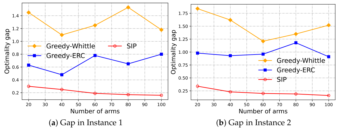
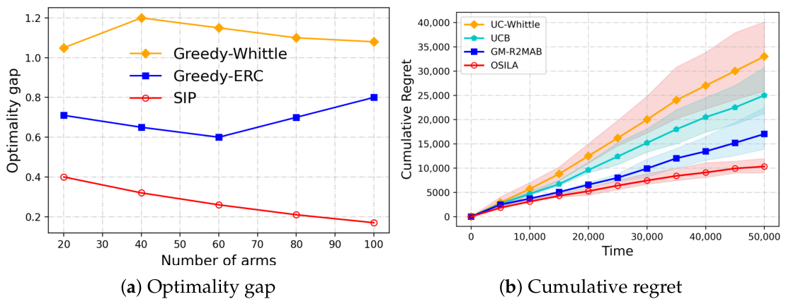
Asymptotic optimality. In the asymptotic optimality analysis of the sleeping index policy, we conducted experiments with T = 50,000 rounds. The optimality gap is defined as the difference between the upper bound of the optimal solution for the S-RMAB problem and the cumulative reward of the index policy. The upper bound of the optimal solution can be obtained by solving the LP problem using Gurobi [51]. We evaluated the variation in the optimality gap for three policies (SIP, greedy-ERC, and greedy-Whittle) as the number of arms increased from 20 to 100. As shown in Figure 1 and Figure 2a, Whittle’s index policy and the ERC policy no longer exhibit asymptotic optimality under the sleeping settings as the number of arms grows. In contrast, the proposed sleeping index policy demonstrates an optimality gap converging to zero, confirming the validity of Theorem 1. This trend is consistent with the theory: greedy-ERC and greedy-Whittle are adapted from non-sleeping RMAB policies and therefore do not account for the structural effect of stochastic arm availability in the oracle construction, whereas SIP is derived directly from the relaxed sleeping LP and explicitly incorporates availability into the index design.
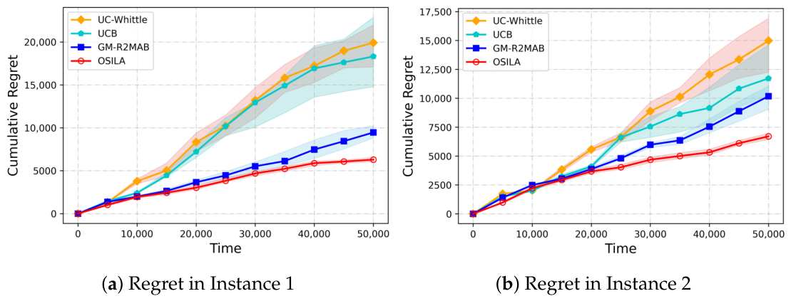
Regret. Under the online setting, we further evaluate the performance of the OSILA. The number of arms is set to K = 20 , and the rounds for each independent experiment vary from 5000 to 50,000. We repeat the independent trials 100 times, and the mean and error range of the algorithm’s cumulative reward are computed. In the regret plots, the solid lines represent the mean values over all repeated experiments, while the shaded regions indicate the fluctuation range across individual trials. As shown in Figure 2b and Figure 3, under the scenario with dynamically changing sets of available arms, the expected regret of our proposed OSILA outperforms GM-R2MAB, UC-Whittle, and UCB algorithms in both problem instances. Specifically, at T = 50,000 rounds, OSILA achieves an average cumulative regret reduction in 35.7% compared to GM-R2MAB, 55.7% against UCB, and 64.1% versus UC-Whittle across three problem instances. This significant improvement stems from OSILA’s high exploration efficiency in dynamic decision spaces — it intelligently allocates sampling resources to rapidly estimate restless state transitions while minimizing wasted explorations on unavailable arms, thereby adapting more effectively to stochastic availability patterns. Furthermore, the cumulative regret of OSILA exhibits a sub-linear growth pattern with increasing rounds. This confirms that the OSILA effectively addresses the online sleeping restless bandits problem.
From a qualitative perspective, the performance gain comes from both components of OSILA, but their roles are slightly different across baselines. Compared with UCB, the main advantage comes from the online sleeping index construction, since UCB does not exploit the restless state dynamics and therefore cannot prioritize arms according to long-term state-dependent value. In contrast, compared with UC-Whittle and GM-R2MAB, which already use RMAB-style indices but are designed for non-sleeping settings, the larger gain mainly comes from the availability-aware exploration mechanism and the sleeping-aware exploitation rule working together. MEG prevents low-availability arms from being persistently under-explored, while the online sleeping index uses the learned availability information to rank only the currently available arms more appropriately. In this sense, the strongest empirical gains of OSILA come from the joint effect of availability-aware exploration and sleeping-aware index construction, rather than from either component alone.

7. Conclusions

This paper is the first to study the online sleeping RMAB problem motivated by dynamic edge-intelligent systems with stochastic arm availability and restless state evolution. We first derive a sleeping-index policy as the oracle through fluid relaxation and establish its asymptotic optimality. Building on this oracle, we then propose OSILA, which combines the Minimum Exploration Guarantee mechanism with an online sleeping-index construction to handle unknown transitions, rewards, and availabilities. On the theoretical side, we characterize the stochastic exploration length and prove a regret bound of O ˜ ( K T 2 / 3 log T ) . On the empirical side, experiments on CPAP intervention planning and AoI optimization in edge-intelligent systems validate both the oracle behavior and the practical effectiveness of OSILA against representative baselines. Future work includes extending the framework to correlated availabilities and non-stationary environments.

Author Contributions

Conceptualization, S.S. and C.F.; methodology, S.S.; software, S.S.; validation, S.S.; formal analysis, S.S.; investigation, S.S. and C.F.; resources, Y.X.; data curation, S.S. and Y.X.; writing—original draft preparation, S.S.; writing—review and editing, S.S., C.F., Y.X., and W.W.; visualization, S.S.; supervision, C.F. and W.W.; project administration, Y.X.; funding acquisition, Y.X. All authors have read and agreed to the published version of the manuscript.

Funding

This research was funded by China Postdoctoral Science Foundation grant number 2025M784430.

Data Availability Statement

The original contributions presented in this study are included in the article. Further inquiries can be directed to the corresponding author.

Conflicts of Interest

Author Dr. Yuhang Xu was employed by the company “North Information Control Research Academy Group Co., Ltd”. The remaining authors declare that the research was conducted in the absence of any commercial or financial relationships that could be construed as a potential conflict of interest.

Appendix A. Main Variables

The main variables used in this paper are summarized in Table A1.
Table A1. Main Variables.
VariableDescription
KNumber of arms
TTotal number of time steps
S State space
A Action space
MBudget constraint on the number of active arms
z i Availability probability of arm i
I t Set of available arms at time t
r ¯ ( s i , a i ) Expected reward for arm i in state s i with action a i
P ( s i , a i , s i ) Transition probability from s i to s i under action a i
π Policy
J π Long-term average reward under policy π
x s i , a i π ( t ) Probability of arm i being in state s i and taking action a i at time t
G ( T ) Number of exploration rounds per arm
r ^ , P ^ , z ^ Estimated reward, transition probability, and availability probability

Appendix B. Equivalent and Modified Linear Programming Problems

In this section, we first provide the construction details for the equivalent transformation of the relaxed S-RMAB into a Linear Programming (LP) formulation. Given the stationary probabilities x ˜ s i , a i π = lim T E π [ t : i I t I { s i ( t ) = s i , a i ( t ) = a i } ] t I { i I t } and the equilibrium condition, we can construct the following LP problem:
max x ˜ s i , a i π i = 1 K z i s i S r ¯ ( s i , 0 ) x ˜ s i , 0 π + r ¯ ( s i , 1 ) x ˜ s i , 1 π ,
s . t . a i A s i S P ( s i , a i , s i ) z i x ˜ s i , a i π = a i A s i S P ( s i , a i , s i ) z i x ˜ s i , a i π i ,
i = 1 K z i s i S x ˜ s i , 1 π M ,
s i S a i A x ˜ s i , a i π = 1 , x ˜ s i , a i π 0 , i , s i , a i .
In the online setting, precise parameters (e.g., r i , P i , z i ) are unknown, making direct LP (Equation (A1)) infeasible. To address this, we reformulate the LP by introducing auxiliary variables y ˜ . This reformulates the problem into the MLP ( r ^ i , P ^ i , z ^ i ) , which depends only on estimates (sampled using the MEG mechanism) and decision variables y ˜ . The details are as follows:
max y ˜ ( s i , a i , s i ) i = 1 K ( s i , a i ) s i S r ^ ( s i , a i ) + ϵ P , r y ˜ ( s i , a i , s i ) ,
s . t . a i A s i S y ˜ ( s i , a i , s i ) = a i A s i S y ˜ ( s i , a i , s i ) ,
i = 1 K s i S s i S y ˜ ( s i , 1 , s i ) M ,
( s i , a i ) s i S y ˜ ( s i , a i , s i ) = z ^ i ,
y ˜ ( s i , a i , s i ) s i S y ˜ ( s i , a i , s i ) P ^ i ϵ P , r .
We choose the Upper Confidence Bounds (UCB) estimators for r ^ ( s i , a i ) , as shown in Equation (A2a). As s i P ( s i , a i , s i ) = 1 , we have s i S y ˜ ( s i , a i , s i ) = s i S P ( s i , a i , s i ) z i x ˜ s i , a i π = z i x ˜ s i , a i π , we can reformulate the equilibrium condition, as shown in Equation (A2b). Similarly, the constructed auxiliary variable y ˜ enables the transformation of constraints Equation (A1c) and Equation (A1d) into Equation (A2c) and Equation (A2d). We expect the solution to the modified LP to remain within the confidence interval. Based on y ˜ ( s i , a i , s i ) / s i S y ˜ ( s i , a i , s i ) = P i , and | P ^ i P i | ϵ P , r , we have Equation (A2e).

Appendix C. Details of the Numerical Case-Study

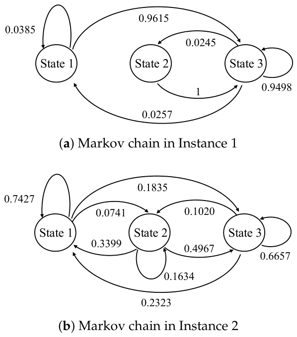
Continuous Positive Airway Pressure (CPAP) Therapy is highly effective for obstructive sleep apnea when used consistently [17,41,49]. However, patient non-adherence reduces its efficacy. We model CPAP adherence behavior as a two-state system (“Adherence” and “Non-Adherence”), based on a three-level clinical adherence scale (states 1 = low, 2 = intermediate, 3 = acceptable). Patients in the “Adherence” state have a higher probability of maintaining acceptable adherence (state 3). Transition probabilities between states differ between the two adherence clusters, as shown in Figure A1.
Figure A1. State transition probability for CPAP.
Symmetry 18 00951 g0a1
For each CPAP instance, the state space is S = { 1 , 2 , 3 } , and the reward values for each arm under different states and actions follow a uniform distribution with means of 0.3, 0.6, and 0.9. The availability probabilities of the arms are independently drawn from the interval [ 0.1 , 0.9 ] . The budget is set to M = 0.3 K .
Freshness optimization in edge-intelligent systems. Consider an edge server gathering real-time sensory data from K edge devices (sources) over M unreliable communication channels to support time-sensitive intelligent tasks. The decision maker needs to select devices for transmission in each round t [ T ] . We define an indicator variable a i ( t ) { 0 , 1 } to represent whether device i is selected in round t. A successful scheduling can occur only when the device has sufficient energy. In this process, devices can harvest energy from ambient source such as solar or wind power. The energy harvesting process is typically modeled as a Bernoulli process [12,19,40], where energy is harvested in each round with probability z i . Specifically, each device has a unit-sized battery, and both the harvested and consumed energy are fixed to one unit. Additionally, a unit of energy is depleted in each round, irrespective of whether the device is scheduled for transmission. Given the limited and unstable channel availability, the decision maker must comply with constraint i a i ( t ) M at each round, while transmissions are subject to a failure probability of 1 p i . The goal of the system is to ensure that the collected data is as fresh as possible.
To measure information freshness, we use the Age of Information (AoI) [9,52], defined as the time elapsed since the generation time-stamp of the freshest information at the receiver. Let h i ( t ) be the AoI of device i at round t, evolving as follows:
h i ( t + 1 ) = h i ( t ) + 1 , transmission failure 1 , otherwise .
Accordingly, the above problem can be formulated as an SRMAB problem, i.e.,
min π lim T 1 T E π [ i t h i ( t ) ] , subject to i a i ( t ) M .
Subsequently, we construct an instance under this problem setting. Consider that the age of each device i is bounded by a constant h m a x = 5 . Then, the state space for each device is S = { 1 , 2 , , h m a x } . The state transition probabilities can be described as follows:
Pr { h i ( t + 1 ) | h i ( t ) , a i ( t ) = 0 } = I { h i ( t + 1 ) = min { h i ( t ) + 1 , h m a x } } Pr { h i ( t + 1 ) | h i ( t ) , a i ( t ) = 1 } = p i , h i ( t + 1 ) = 1 1 p i , h i ( t + 1 ) = min { h i ( t ) + 1 , h m a x }
The reward of each device is negatively correlated with its AoI and follows a uniform distribution with means of 0.8, 0.7, 0.6, 0.5, and 0.4, respectively. The energy arrival probabilities z i and channel transmission probabilities p i are independently drawn from the interval [ 0.1 , 0.9 ] . The budget is set to M = 0.3 K .

References

  1. Ji, C.; Wu, F.; Zhu, Z.; Chang, L.P.; Liu, H.; Zhai, W. Memory-efficient deep learning inference with incremental weight loading and data layout reorganization on edge systems. J. Syst. Archit. 2021, 118, 102183. [Google Scholar] [CrossRef] [Scilit]
  2. Ji, C.; Pan, R.; Chang, L.P.; Shi, L.; Zhu, Z.; Liang, Y.; Kuo, T.W.; Xue, C.J. Inspection and Characterization of App File Usage in Mobile Devices. ACM Trans. Storage 2020, 16, 1–25. [Google Scholar] [CrossRef] [Scilit]
  3. Raeisi-Varzaneh, M.; Dakkak, O.; Habbal, A.; Kim, B.S. Resource scheduling in edge computing: Architecture, taxonomy, open issues and future research directions. IEEE Access 2023, 11, 25329–25350. [Google Scholar] [CrossRef] [Scilit]
  4. Avan, A.; Azim, A.; Mahmoud, Q.H. A state-of-the-art review of task scheduling for edge computing: A delay-sensitive application perspective. Electronics 2023, 12, 2599. [Google Scholar] [CrossRef] [Scilit]
  5. Fan, W.; Liu, X.; Yuan, H.; Li, N.; Liu, Y. Time-slotted task offloading and resource allocation for cloud-edge-end cooperative computing networks. IEEE Trans. Mob. Comput. 2024, 23, 8225–8241. [Google Scholar] [CrossRef] [Scilit]
  6. Xu, C.; Guo, J.; Li, Y.; Zou, H.; Jia, W.; Wang, T. Dynamic parallel multi-server selection and allocation in collaborative edge computing. IEEE Trans. Mob. Comput. 2024, 23, 10523–10537. [Google Scholar] [CrossRef] [Scilit]
  7. Chen, Z.; Xiong, B.; Chen, X.; Min, G.; Li, J. Joint computation offloading and resource allocation in multi-edge smart communities with personalized federated deep reinforcement learning. IEEE Trans. Mob. Comput. 2024, 23, 11604–11619. [Google Scholar] [CrossRef] [Scilit]
  8. Whittle, P. Restless bandits: Activity allocation in a changing world. J. Appl. Probab. 1988, 25, 287–298. [Google Scholar] [CrossRef] [Scilit]
  9. Kadota, I.; Sinha, A.; Uysal-Biyikoglu, E.; Singh, R.; Modiano, E. Scheduling policies for minimizing age of information in broadcast wireless networks. IEEE/ACM Trans. Netw. 2018, 26, 2637–2650. [Google Scholar] [CrossRef] [Scilit]
  10. Maatouk, A.; Kriouile, S.; Assad, M.; Ephremides, A. On the optimality of the Whittle’s index policy for minimizing the age of information. IEEE Trans. Wirel. Commun. 2020, 20, 1263–1277. [Google Scholar] [CrossRef] [Scilit]
  11. Xiong, G.; Wang, S.; Yan, G.; Li, J. Reinforcement learning for dynamic dimensioning of cloud caches: A restless bandit approach. IEEE/ACM Trans. Netw. 2023, 31, 2147–2161. [Google Scholar] [CrossRef] [Scilit]
  12. Sun, S.; Wu, W.; Fu, C.; Qiu, X.; Luo, J.; Wang, J. AoI Optimization in Multi-source Update Network Systems under Stochastic Energy Harvesting Model. IEEE J. Sel. Areas Commun. 2024, 42, 3172–3187. [Google Scholar] [CrossRef] [Scilit]
  13. Mate, A.; Perrault, A.; Tambe, M. Risk-Aware Interventions in Public Health: Planning with Restless Multi-Armed Bandits. In Proceedings of the AAMAS, Virtual, 3–7 May 2021; pp. 880–888. [Google Scholar]
  14. Ortner, R.; Ryabko, D.; Auer, P.; Munos, R. Regret bounds for restless markov bandits. In International Conference on Algorithmic Learning Theory; Springer: Berlin/Heidelberg, Germany, 2012; pp. 214–228. [Google Scholar]
  15. Wang, S.; Huang, L.; Lui, J. Restless-UCB, an efficient and low-complexity algorithm for online restless bandits. Adv. Neural Inf. Process. Syst. 2020, 33, 11878–11889. [Google Scholar]
  16. Wang, K.; Xu, L.; Taneja, A.; Tambe, M. Optimistic whittle index policy: Online learning for restless bandits. In Proceedings of the AAAI Conference on Artificial Intelligence, Washington, DC, USA, 7–14 February 2023; Volume 37, pp. 10131–10139. [Google Scholar]
  17. Xiong, G.; Li, J. Provably Efficient Reinforcement Learning for Adversarial Restless Multi-Armed Bandits with Unknown Transitions and Bandit Feedback. In Proceedings of the Forty-First International Conference on Machine Learning, Vienna, Austria, 21–27 July 2024. [Google Scholar]
  18. Kadota, I.; Modiano, E. Minimizing the Age of Information in Wireless Networks with Stochastic Arrivals. IEEE Trans. Mob. Comput. 2021, 20, 1173–1185. [Google Scholar] [CrossRef]
  19. Hatami, M.; Codreanu, M. On the age-optimality of relax-then-truncate approach under partial battery knowledge in energy harvesting IoT networks. In 2023 21st International Symposium on Modeling and Optimization in Mobile, Ad Hoc, and Wireless Networks (WiOpt); IEEE: New York, NY, USA, 2023; pp. 589–596. [Google Scholar]
  20. Chen, G.; Liew, S.C.; Shao, Y. Uncertainty-of-information scheduling: A restless multiarmed bandit framework. IEEE Trans. Inf. Theory 2022, 68, 6151–6173. [Google Scholar] [CrossRef] [Scilit]
  21. Kleinberg, R.; Niculescu-Mizil, A.; Sharma, Y. Regret bounds for sleeping experts and bandits. Mach. Learn. 2010, 80, 245–272. [Google Scholar] [CrossRef] [Scilit]
  22. Saha, A.; Gaillard, P.; Valko, M. Improved sleeping bandits with stochastic action sets and adversarial rewards. In International Conference on Machine Learning; PMLR: Cambridge, MA, USA, 2020; pp. 8357–8366. [Google Scholar]
  23. Nguyen, Q.M.; Mehta, N. Near-optimal per-action regret bounds for sleeping bandits. In International Conference on Artificial Intelligence and Statistics; PMLR: Cambridge, MA, USA, 2024; pp. 2827–2835. [Google Scholar]
  24. Verloop, I. Asymptotically optimal priority policies for indexable and nonindexable restless bandits. Ann. Appl. Probab. 2016, 26, 1947–1995. [Google Scholar] [CrossRef] [Scilit]
  25. Xiong, G.; Wang, S.; Li, J. Learning infinite-horizon average-reward restless multi-action bandits via index awareness. Adv. Neural Inf. Process. Syst. 2022, 35, 17911–17925. [Google Scholar]
  26. Blum, A. Empirical support for winnow and weighted-majority algorithms: Results on a calendar scheduling domain. Mach. Learn. 1997, 26, 5–23. [Google Scholar] [CrossRef] [Scilit]
  27. Freund, Y.; Schapire, R.E.; Singer, Y.; Warmuth, M.K. Using and combining predictors that specialize. In Proceedings of the Twenty-Ninth Annual ACM Symposium on Theory of Computing, El Paso, TX, USA, 4–6 May 1997; pp. 334–343. [Google Scholar]
  28. Blum, A.; Mansour, Y. From external to internal regret. J. Mach. Learn. Res. 2007, 8, 1307–1324. [Google Scholar]
  29. Kanade, V.; Steinke, T. Learning hurdles for sleeping experts. ACM Trans. Comput. Theory (TOCT) 2014, 6, 1–16. [Google Scholar] [CrossRef] [Scilit]
  30. Kanade, V.; McMahan, H.B.; Bryan, B. Sleeping experts and bandits with stochastic action availability and adversarial rewards. In Artificial Intelligence and Statistics; PMLR: Cambridge, MA, USA, 2009; pp. 272–279. [Google Scholar]
  31. Gaillard, P.; Saha, A.; Dan, S. One arrow, two kills: A unified framework for achieving optimal regret guarantees in sleeping bandits. In International Conference on Artificial Intelligence and Statistics; PMLR: Cambridge, MA, USA, 2023; pp. 7755–7773. [Google Scholar]
  32. Neu, G.; Valko, M. Online combinatorial optimization with stochastic decision sets and adversarial losses. Adv. Neural Inf. Process. Syst. 2014, 27, 2780–2788. [Google Scholar]
  33. Kale, S.; Lee, C.; Pál, D. Hardness of online sleeping combinatorial optimization problems. Adv. Neural Inf. Process. Syst. 2016, 29, 2189–2197. [Google Scholar]
  34. Li, F.; Liu, J.; Ji, B. Combinatorial sleeping bandits with fairness constraints. IEEE Trans. Netw. Sci. Eng. 2019, 7, 1799–1813. [Google Scholar] [CrossRef] [Scilit]
  35. Papadimitriou, C.H.; Tsitsiklis, J.N. The complexity of optimal queuing network control. Math. Oper. Res. 1999, 24, 293–305. [Google Scholar] [CrossRef] [Scilit]
  36. Weber, R.R.; Weiss, G. On an index policy for restless bandits. J. Appl. Probab. 1990, 27, 637–648. [Google Scholar] [CrossRef] [Scilit]
  37. Akbarzadeh, N.; Mahajan, A. Restless bandits with controlled restarts: Indexability and computation of Whittle index. In 2019 IEEE 58th Conference on Decision and Control (CDC); IEEE: New York, NY, USA, 2019; pp. 7294–7300. [Google Scholar]
  38. Xiong, G.; Li, J.; Singh, R. Reinforcement learning augmented asymptotically optimal index policy for finite-horizon restless bandits. In Proceedings of the AAAI Conference on Artificial Intelligence, Online, 22 February–1 March 2022; Volume 36, pp. 8726–8734. [Google Scholar]
  39. Jiang, B.; Jiang, B.; Li, J.; Lin, T.; Wang, X.; Zhou, C. Online restless bandits with unobserved states. In International Conference on Machine Learning; PMLR: Cambridge, MA, USA, 2023; pp. 15041–15066. [Google Scholar]
  40. Hatami, M.; Leinonen, M.; Chen, Z.; Pappas, N.; Codreanu, M. On-demand AoI minimization in resource-constrained cache-enabled IoT networks with energy harvesting sensors. IEEE Trans. Commun. 2022, 70, 7446–7463. [Google Scholar] [CrossRef] [Scilit]
  41. Wang, S.; Xiong, G.; Li, J. Online restless multi-armed bandits with long-term fairness constraints. In Proceedings of the AAAI Conference on Artificial Intelligence, Vancouver, BC, Canada, 20–28 February 2024; Volume 38, pp. 15616–15624. [Google Scholar]
  42. Puterman, M.L. Markov Decision Processes: Discrete Stochastic Dynamic Programming; John Wiley & Sons: Hoboken, NJ, USA, 2014. [Google Scholar]
  43. Ethier, S.N.; Kurtz, T.G. Markov Processes: Characterization and Convergence; John Wiley & Sons: Hoboken, NJ, USA, 2009. [Google Scholar]
  44. Gast, N.; Bruno, G. A mean field model of work stealing in large-scale systems. ACM SIGMETRICS Perform. Eval. Rev. 2010, 38, 13–24. [Google Scholar] [CrossRef] [Scilit]
  45. Besbes, O.; Gur, Y.; Zeevi, A. Stochastic multi-armed-bandit problem with non-stationary rewards. Adv. Neural Inf. Process. Syst. 2014, 27, 199–207. [Google Scholar]
  46. Cheung, W.C.; Simchi-Levi, D.; Zhu, H. Learning to optimize under non-stationarity. In The 22nd International Conference on Artificial Intelligence and Statistics; PMLR: Cambridge, MA, USA, 2019; pp. 1079–1087. [Google Scholar]
  47. Ortner, R.; Gajane, P.; Auer, P. Variational regret bounds for reinforcement learning. In Uncertainty in Artificial Intelligence; PMLR: Cambridge, MA, USA, 2020; pp. 81–90. [Google Scholar]
  48. Hoeffding, W. Probability inequalities for sums of bounded random variables. In The Collected Works of Wassily Hoeffding; Springer: New York, NY, USA, 1994; pp. 409–426. [Google Scholar]
  49. Herlihy, C.; Prins, A.; Srinivasan, A.; Dickerson, J.P. Planning to fairly allocate: Probabilistic fairness in the restless bandit setting. In Proceedings of the 29th ACM SIGKDD Conference on Knowledge Discovery and Data Mining, Long Beach, CA, USA, 6–10 August 2023; pp. 732–740. [Google Scholar]
  50. Lattimore, T.; Szepesvári, C. Bandit Algorithms; Cambridge University Press: Cambridge, UK, 2020. [Google Scholar]
  51. Gurobi Optimization, LLC. Gurobi Optimizer Reference Manual; Gurobi Optimization, LLC: Beaverton, OR, USA, 2024. [Google Scholar]
  52. Sun, Y.; Uysal-Biyikoglu, E.; Yates, R.D.; Koksal, C.E.; Shroff, N.B. Update or wait: How to keep your data fresh. IEEE Trans. Inf. Theory 2017, 63, 7492–7508. [Google Scholar] [CrossRef] [Scilit]
Figure 1. Optimality gap for CPAP application.
Symmetry 18 00951 g001
Figure 2. Performance comparison for case study AoI optimization in edge intelligent systems.
Symmetry 18 00951 g002
Figure 3. Regret for CPAP application.
Symmetry 18 00951 g003
Disclaimer/Publisher’s Note: The statements, opinions and data contained in all publications are solely those of the individual author(s) and contributor(s) and not of MDPI and/or the editor(s). MDPI and/or the editor(s) disclaim responsibility for any injury to people or property resulting from any ideas, methods, instructions or products referred to in the content.