Optimal Transformation-Based Median Estimation Under Stratified Double Sampling with Limited Auxiliary Information

Abstract

This study develops a new class of transformation-based estimators for estimating the population median within a stratified two-phase sampling framework. The proposed approach is designed to improve estimation accuracy while reducing survey costs, particularly in situations where auxiliary information is partially available or expensive to collect. By using suitable transformations of the auxiliary variable, the estimators achieve greater stability and robustness in the presence of skewed distributions and extreme observations. Theoretical properties of the proposed estimators are established using first-order approximations, leading to explicit expressions for bias and mean squared error. Optimal conditions are also derived to ensure improved efficiency. To evaluate performance, both simulation experiments and real-world datasets are considered under a variety of distributional settings and correlation structures. The results consistently show that the proposed estimators outperform conventional approaches, including ratio, regression, and exponential-type estimators, in terms of efficiency. In particular, notable improvements are observed for skewed and heavy-tailed populations, where traditional methods often perform poorly. These findings highlight the practical usefulness of the proposed methodology for survey applications in fields such as economics, public health, and social sciences, where reliable median estimation is essential.

1. Introduction

A sampling design can be particularly costly when attempting to obtain accurate estimates in survey research, especially when the population is skewed or contains extreme values. In such cases, the median is a more appropriate measure of central tendency than the arithmetic mean, which may produce unreliable results. Median-based analysis has become widely used in many fields, including monitoring computer network traffic, studying species distribution in ecology, and evaluating public policies, where extreme responses can significantly influence average outcomes. As a practical extension of stratification methods, stratified two-phase sampling balances estimation accuracy with survey economy. In economic surveys, stratifying data by employment status provides reliable estimates of median income, while grouping individuals by age or disease severity in health studies improves the estimation of median recovery times. Therefore, the advantages of this approach are evident in practical applications. These applications demonstrate the effectiveness of stratified two-phase sampling as a reliable method for conducting surveys. Further details regarding the use of auxiliary information can be found in [1,2].

The problem of population median estimation has attracted considerable attention in survey sampling, particularly when dealing with skewed populations and extreme observations. Important theoretical results on linear functions of order statistics were presented in [3], which later provided the basis for many developments in median estimation. The practical importance of median estimation in sample surveys was discussed in [4], while confidence interval procedures for finite population quantiles under simple and stratified random sampling were developed in [5]. Further investigations on lower bounds for confidence coefficients associated with interval estimation of finite population quantiles were carried out in [6]. The role of auxiliary information in improving population median estimation was later demonstrated in [7]. Improved ratio and regression estimation methods were introduced in [8], motivating several subsequent contributions in survey sampling theory. Extensions of median estimation to double sampling frameworks were studied in [9], whereas a generalized class of estimators using two auxiliary variables in double sampling was proposed in [10]. Additional theoretical developments and applications in sampling theory were presented in [11]. Later, median estimation procedures under two-phase sampling using two auxiliary variables were proposed in [12], leading to substantial improvements in estimation efficiency.

Further advancements in population median estimation have focused on improving efficiency and robustness through the effective use of auxiliary information. Improvements in estimating the population median under both simple random and stratified random sampling were presented in [13]. Several flexible classes of estimators for median estimation in survey sampling were later proposed in [14], providing alternative approaches for achieving higher estimation accuracy. More recently, simulation-based studies on auxiliary variable methods for population median estimation using real data across different sample sizes were conducted in [15]. A family of estimators utilizing auxiliary information for improved population median estimation was introduced in [16], whereas improved difference-type estimators for survey sampling applications were proposed in [17]. Generalized classes of median estimators based on auxiliary variables were further developed in [18], while robust auxiliary measures for neutrosophic finite median estimation were explored in [19]. The balance between estimation accuracy and survey cost under stratified random sampling was emphasized in [20]. In addition, improved and robust difference-type estimators for population median estimation were discussed in [21,22,23]. Efficient ratio-cum-median estimators were proposed in [24], whereas efficiency considerations under fixed survey cost conditions were examined in [25]. Furthermore, robust stratified median estimation procedures based on auxiliary transformations and nontraditional auxiliary measures for asymmetric populations were introduced in [26].

For skewed or non-normal populations, conventional estimators such as ratio, regression, exponential, and product estimators often become unreliable because they rely on distributional symmetry and are highly sensitive to extreme observations. To overcome the limitations highlighted in [15], the present study introduces transformation-based estimators within a stratified two-phase random sampling framework to improve estimation accuracy and stability. Since the median provides a more robust measure of central tendency and the auxiliary information collected during the first phase enhances estimation efficiency, the proposed procedures are particularly useful in variable situations such as weather-dependent agricultural yields, manufacturing processes involving defective items, and highly skewed educational outcomes.

The proposed class of estimators offers several distinct contributions to survey methodology. Its distributional adaptability ensures reliable performance in skewed or non-normal populations, where conventional estimators often fail. The proposed approach is also resistant to outliers, making it less vulnerable to extreme values and thereby improving estimation accuracy in real-world data settings. The stratified two-phase sampling design reduces overall survey cost without compromising precision by effectively utilizing supplementary information collected during the first phase. In addition, the transformation-enhanced approach outperforms traditional ratio and regression estimators in terms of relative efficiency. The generalizability of the proposed method further extends its applicability to various fields where accurate median estimation is important, including income analysis, healthcare, and agriculture. Furthermore, both simulation studies and real datasets demonstrate cross-distributional consistency, confirming that the proposed estimators are reliable and stable under different statistical conditions.

Although the present work is motivated by earlier transformation-based median estimation procedures, the current study extends the methodology to a substantially more complex stratified two-phase sampling framework. Unlike conventional single-stage or simple two-phase settings, the proposed approach adopts independent first-phase and second-phase sampling within each stratum, requiring separate derivations of bias, mean squared error, and optimal parameter conditions under stratified double sampling.

The proposed framework further combines stratum-specific auxiliary transformations to improve robustness and efficiency in heterogeneous populations where auxiliary information may be partially available or expensive to obtain. In addition, the study develops a generalized family of estimators containing several transformation sub classes and evaluates their performance under skewed and heavy-tailed distributions as well as real population datasets. These extensions considerably broaden the practical applicability of transformation-based median estimation under complex survey designs.

Practical Implementation and Applicability of the Proposed Estimators

The proposed class of transformation-based estimators is designed not only to improve theoretical efficiency but also to provide practical applicability in real survey situations where auxiliary information may be partially available or costly to obtain. The estimators can be implemented using standard statistical software such as R, MATLAB, SPSS, or Python without requiring complicated computational procedures. Since the methodology is based on sample medians, auxiliary transformations, and first-order approximations, the implementation process remains computationally manageable even for moderately large populations.

In practical applications, the first-phase sample can be used to collect inexpensive auxiliary information, while the second-phase sample is utilized for obtaining both study and auxiliary variables. This structure is especially useful in large-scale surveys where complete information on the study variable is difficult, time-consuming, or expensive to obtain. The proposed estimators therefore offer an effective balance between estimation precision and survey cost.

An additional advantage of the proposed methodology is its flexibility under different population structures. The transformation parameters introduced in the estimator family allow the method to adapt efficiently to skewed, heavy-tailed, and heterogeneous populations where traditional ratio and regression estimators may lose efficiency. The simulation and empirical analyses presented in this study demonstrate that the estimators maintain stable performance across different correlation levels and distributional settings.

Furthermore, the proposed estimators can be applied in a wide range of practical fields including health surveys, economic investigations, agricultural studies, educational assessments, and social science research, where robust estimation of the population median is often more appropriate than mean-based estimation. The improved efficiency and stability observed in both simulated and real datasets indicate that the proposed methodology can serve as a reliable alternative to existing median estimators under stratified two-phase sampling designs.

2. Notation and Symbols

This section presents the notation and general framework used for median estimation. Consider a finite population of size N denoted by:

$$\Omega =\{{\Omega }_1,{\Omega }_2,{\Omega }_3,\dots ,{\Omega }_N\}.$$

The population is subdivided into L non-overlapping and exhaustive strata, where stratum h contains $N_h$ units, and is expressed as:

$${\displaystyle \sum _{h=1}^L}{N}_h=N.$$

where Y denotes the study variable of interest and X denotes an auxiliary variable used to improve the accuracy of the estimates. Simple random samples of size $m_h$ are independently drawn without replacement from each stratum, and these are combined to obtain the total sample size in phase l:

$$X_{1h}=\{x_{1h},x_{2h},\dots ,x_{mh}\}$$

and

$${\displaystyle \sum _{h=1}^L}{m}_h=m.$$

The observations at the initial sampling phase are measured for the auxiliary variable X. These observations are then used to approximate the population median of X, denoted by $M_x$, based on the sampled values.

The sample observations in phase II,

$$X_{2h}=\{x_{1h},x_{2h},\dots ,x_{nh}\},$$

are then selected by drawing $n_h$ units from each first-phase sample within each stratum using SRSWOR, where

$${\displaystyle \sum _{h=1}^L}{n}_h=n.$$

At this phase of the survey, information is gathered simultaneously for the study variable Y and the auxiliary variable $X.$

Let the hth stratum’s population medians be denoted by $M_{yh}$ and $M_{xh},$ respectively. Their two-phase sample estimates are ${\widehat{M}}_{x_{1h}},{\widehat{M}}_{x_{2h}},$ and ${\widehat{M}}_{yh}$. The probability densities at the respective medians in the hth stratum are represented by $f_{yh}\left(M_{yh}\right)$ and $f_{xh}\left(M_{xh}\right)$. The relationship between these medians is defined by

$${\rho }_{x_h{y}_h}(M_{xh},M_{yh})=4Q_{11h}(x_h,y_h)-1,$$

with $Q_{11h}$ representing the probability that

$$Q(x_h\le M_{xh},y_h\le M_{yh}).$$

A basic framework for determining bias and mean squared error is provided by the following expressions, which relate relative errors to their corresponding expected values. These formulations are important for evaluating the accuracy and reliability of estimators, as they allow researchers to approximate the expected deviation from the true population parameter while accounting for sampling variability.

$${\Delta }_{0h}=\left({\displaystyle \frac{{\widehat{M}}_{yh}-M_{yh}}{M_{yh}}}\right),$$

$${\Delta }_{1h}=\left({\displaystyle \frac{{\widehat{M}}_{x_{1h}}-M_{xh}}{M_{xh}}}\right)$$

and

$${\Delta }_{2h}=\left({\displaystyle \frac{{\widehat{M}}_{x2h}-M_{xh}}{M_{xh}}}\right),$$

such that $E\left({\Delta }_{ih}\right)=0$ for $i=0,1,2$.

Further,

$$E\left({\Delta }_{0h}^2\right)={\delta }_{1h}{C}_{M_{yh}}^2,$$

$$E\left({\Delta }_{1h}^2\right)={\delta }_{2h}{C}_{M_{xh}}^2,$$

$$E\left({\Delta }_{2h}^2\right)={\delta }_{1h}{C}_{M_{xh}}^2,$$

$$E\left({\Delta }_{0h}{\Delta }_{1h}\right)={\delta }_{2h}{C}_{M_{yxh}}={\rho }_{yxh}{C}_{M_{yh}}{C}_{M_{xh}},$$

$$E\left({\Delta }_{0h}{\Delta }_{2h}\right)={\delta }_{1h}{C}_{M_{yxh}}={\rho }_{yxh}{C}_{M_{yh}}{C}_{M_{xh}},$$

$$E\left({\Delta }_{1h}{\Delta }_{2h}\right)={\delta }_{2h}{C}_{M_{xh}}^2,$$

where

$$C_{M_{yh}}={\displaystyle \frac{1}{M_{yh}{f}_{yh}\left(M_{yh}\right)}},$$

$$C_{M_{xh}}={\displaystyle \frac{1}{M_{xh}{f}_{xh}\left(M_{xh}\right)}},$$

$${\delta }_{1h}={\displaystyle \frac{1}{4}}\left({\displaystyle \frac{1}{n_h}}-{\displaystyle \frac{1}{N_h}}\right),$$

$${\delta }_{2h}={\displaystyle \frac{1}{4}}\left({\displaystyle \frac{1}{m_h}}-{\displaystyle \frac{1}{N_h}}\right),$$

$${\delta }_{3h}={\displaystyle \frac{1}{4}}\left({\displaystyle \frac{1}{n_h}}-{\displaystyle \frac{1}{m_h}}\right).$$

3. Review of Conventional Estimators

The median estimators developed in the literature perform differently depending on the sampling design and population structure. This section provides a thorough analysis of these estimators, emphasizing their theoretical properties such as variance, bias, and mean squared error. Examining these methods not only provides a basis for comparison but also highlights the limitations of existing approaches, thereby laying the groundwork for the development of improved and more efficient estimation methods.

Using the stratified two-phase sampling approach, the conventional sample median estimator and associated variance expression are defined as follows, initially introduced by [4]:

$${\widehat{D}}_{1st}={\displaystyle \sum _{h=1}^L}{W}_h{\widehat{M}}_{y_h}$$

(1)

and

$$Var\left({\widehat{D}}_{1st}\right)={\displaystyle \sum _{h=1}^L}{\delta }_{1h}{W}_h^2{M}_{yh}^2{C}_{M_{yh}}^2.$$

(2)

In this research, we modify the ratio estimator proposed by [9] for double sampling to accommodate stratified double sampling, which is expressed as follows:

$${\widehat{D}}_{2st}={\displaystyle \sum _{h=1}^L}{W}_h\left({\displaystyle \frac{{\widehat{M}}_{yh}}{{\widehat{M}}_{x_{2h}}}}\right){\widehat{M}}_{x_{1h}}.$$

(3)

We can use the following first-order formulas to obtain estimates of ${\widehat{D}}_{2st}$:

$$Bias\left({\widehat{D}}_{2st}\right)\cong {\displaystyle \sum _{h=1}^L}{W}_h{\delta }_{3h}{M}_{yh}\left(C_{M_{xh}}^2-C_{M_{yxh}}\right)$$

(4)

and

$$MSE\left({\widehat{D}}_{2st}\right)\cong {\displaystyle \sum _{h=1}^L}{W}_h^2{M}_{yh}^2\left[{\delta }_{1h}{C}_{M_{yh}}^2+{\delta }_{3h}\left(C_{M_{xh}}^2-2C_{M_{yxh}}\right)\right].$$

(5)

The difference-type estimator is rewritten using the method of [11] in stratified two-phase sampling. For ${\widehat{D}}_{3st}$, the following expression holds:

$${\widehat{D}}_{3st}={\displaystyle \sum _{h=1}^L}{W}_h\left[{\widehat{M}}_{yh}+d_{1h}\left({\widehat{M}}_{x_{1h}}-{\widehat{M}}_{x_{2h}}\right)\right].$$

(6)

The optimum mean MSE for ${\widehat{D}}_{3st}$ at the best value of $d_{1h}$ using the first-order approximation is as follows:

$$MSE{\left({\widehat{D}}_{3st}\right)}_{min}\cong {\displaystyle \sum _{h=1}^L}{W}_h^2{M}_{yh}^2{C}_{M_{yh}}^2\left({\delta }_{1h}-{\delta }_{3h}{\rho }_{yxh}^2\right),$$

(7)

where

$$d_{1h\left(opt\right)}={\displaystyle \frac{{\rho }_{yxh}{M}_{yh}{C}_{M_{yh}}}{M_{xh}{C}_{M_{xh}}}}.$$

In this work, the exponential estimators proposed by [27] under double sampling are generalized to stratified double sampling as described below:

$${\widehat{D}}_{4st}={\displaystyle \sum _{h=1}^L}{W}_h{\widehat{M}}_{yh}exp\left({\displaystyle \frac{{\widehat{M}}_{x_{1h}}-{\widehat{M}}_{x_{2h}}}{{\widehat{M}}_{x_{1h}}+{\widehat{M}}_{x_{2h}}}}\right)$$

(8)

and

$${\widehat{D}}_{5st}={\displaystyle \sum _{h=1}^L}{W}_h{\widehat{M}}_{yh}exp\left({\displaystyle \frac{{\widehat{M}}_{x_{2h}}-{\widehat{M}}_{x_{1h}}}{{\widehat{M}}_{x_{1h}}+{\widehat{M}}_{x_{2h}}}}\right).$$

(9)

The corresponding formulas are valid under a first-order expansion and can be written as follows:

$$Bias\left({\widehat{D}}_{4st}\right)\cong {\displaystyle \frac{1}{2}}{\displaystyle \sum _{h=1}^L}{W}_h{\delta }_{3h}{M}_{yh}\left({\displaystyle \frac{3}{4}}{C}_{M_{xh}}^2-C_{M_{yxh}}\right),$$

(10)

$$Bias\left({\widehat{D}}_{5st}\right)\cong {\displaystyle \frac{1}{2}}{\displaystyle \sum _{h=1}^L}{W}_h{\delta }_{3h}{M}_{yh}\left({\displaystyle \frac{3}{4}}{C}_{M_{xh}}^2+C_{M_{yxh}}\right),$$

(11)

$$MSE\left({\widehat{D}}_{4st}\right)\cong {\displaystyle \sum _{h=1}^L}{W}_h^2{M}_{yh}^2\left[{\delta }_{1h}{C}_{M_{yh}}^2+{\delta }_{3h}{C}_{M_{xh}}^2\left({\displaystyle \frac{1}{4}}-T_h\right)\right]$$

(12)

and

$$MSE\left({\widehat{D}}_{5st}\right)\cong {\displaystyle \sum _{h=1}^L}{W}_h^2{M}_{yh}^2\left[{\delta }_{1h}{C}_{M_{yh}}^2+{\delta }_{3h}{C}_{M_{xh}}^2\left({\displaystyle \frac{1}{4}}+T_h\right)\right],$$

(13)

where

$$T_h={\displaystyle \frac{{\rho }_{yxh}{C}_{M_{yh}}}{C_{M_{xh}}}}.$$

This study is an extension of the work of [8,12], in which estimators were proposed under the two-phase sampling scenario. The stratified formulas can be expressed as follows:

$${\widehat{D}}_{6st}={\displaystyle \sum _{h=1}^L}{W}_h\left[d_{2h}{\widehat{M}}_{yh}+d_{3h}\left({\widehat{M}}_{x_{1h}}-{\widehat{M}}_{x_{2h}}\right)\right],$$

(14)

$${\widehat{D}}_{7st}={\displaystyle \sum _{h=1}^L}{W}_h\left[d_{4h}{\widehat{M}}_{yh}+d_{5h}\left({\widehat{M}}_{x_{1h}}-{\widehat{M}}_{x_{2h}}\right)\right]\left({\displaystyle \frac{{\widehat{M}}_{x_{1h}}}{{\widehat{M}}_{x_{2h}}}}\right),$$

(15)

$${\widehat{D}}_{8st}={\displaystyle \sum _{h=1}^L}{W}_h\left[d_{6h}{\widehat{M}}_{yh}+d_{7h}\left({\widehat{M}}_{x_{1h}}-{\widehat{M}}_{x_{2h}}\right)\right]\left({\displaystyle \frac{{\widehat{M}}_{x_{1h}}-{\widehat{M}}_{x_{2h}}}{{\widehat{M}}_{x_{1h}}+{\widehat{M}}_{x_{2h}}}}\right).$$

(16)

The formulas given below represent the estimators in a stratified two-phase design and can be expressed as follows:

$$Bias{\left({\widehat{D}}_{6st}\right)}_{min}\cong -{\displaystyle \sum _{h=1}^L}{W}_h{M}_{yh}\left[{\displaystyle \frac{{\delta }_{1h}{C}_{M_{yh}}^2{C}_{M_{xh}}^2-{\delta }_{3h}{C}_{M_{yxh}}^2}{C_{M_{xh}}^2\left(1+{\delta }_{1h}{C}_{M_{yh}}^2\right)-{\delta }_{3h}{C}_{M_{yxh}}^2}}\right],$$

(17)

$$\begin{array}{cc}\hfill Bias{\left({\widehat{D}}_{7st}\right)}_{min}\cong {\displaystyle \sum _{h=1}^L}{W}_h[M_{yh}\left(d_{4h\left(opt\right)}-1\right)& +{\delta }_{3h}\{d_{4h\left(opt\right)}{M}_{yh}\left(C_{M_{xh}}^2-C_{M_{yxh}}\right)\hfill \\ \hfill +d_{5h\left(opt\right)}{M}_{xh}{C}_{M_{xh}}^2\left\}\right],& \end{array}$$

(18)

$$Bias{\left({\widehat{D}}_{8st}\right)}_{min}\cong {\displaystyle \sum _{h=1}^L}{W}_h{M}_{yh}\left[-1+{\displaystyle \frac{{\delta }_{3h}}{4}}{C}_{M_x}^2\left\{-1+d_{6h\left(opt\right)}\left({\displaystyle \frac{M_{xh}+8{\rho }_{yxh}{M}_{yh}}{M_{xh}}}\right)\right\}\right],$$

(19)

$$MSE{\left({\widehat{D}}_{6st}\right)}_{min}\cong {\displaystyle \sum _{h=1}^L}{W}_h^2{M}_{yh}^2\left[{\displaystyle \frac{{\delta }_{1h}{C}_{M_{yh}}^2{C}_{M_{xh}}^2-{\delta }_{3h}{C}_{M_{yxh}}^2}{C_{M_{xh}}^2\left(1+{\delta }_{1h}{C}_{M_{yh}}^2\right)-{\delta }_{3h}{C}_{M_{yxh}}^2}}\right],$$

(20)

$$\begin{array}{cc}\hfill MSE{\left({\widehat{D}}_{7st}\right)}_{min}& \cong {\displaystyle \sum _{h=1}^L}{W}_h^2[{\left\{Bias\left({\widehat{D}}_{7st}\right)\right\}}_{min}^2+{\delta }_{1h}{M}_{yh}^2{d}_{4h\left(\mathrm{opt}\right)}^2{C}_{M_{yh}}^2\hfill \\ \hfill & +{\delta }_{3h}\{C_{M_{xh}}^2{\left(d_{4h\left(\mathrm{opt}\right)}{M}_{yh}+d_{5h\left(\mathrm{opt}\right)}{M}_{xh}\right)}^2\hfill \\ \hfill & -2d_{4h\left(\mathrm{opt}\right)}{M}_{yh}{C}_{M_{yxh}}\left(d_{4h\left(\mathrm{opt}\right)}{M}_{yh}+d_{5h\left(\mathrm{opt}\right)}{M}_{xh}\right)\left\}\right]\hfill \end{array}$$

(21)

$$MSE{\left({\widehat{M}}_8\right)}_{min}\cong {\displaystyle \sum _{h=1}^L}{W}_h^2\left[Bias{\left({\widehat{D}}_{8st}\right)}_{min}+{\displaystyle \frac{{\delta }_{3h}}{4}}{d}_{6h\left(opt\right)}^2{M}_{yh}^2{C}_{M_{xh}}^2\right],$$

(22)

where

$$d_{2h\left(opt\right)}={\displaystyle \frac{C_{M_{xh}}^2}{C_{M_{xh}}^2\left(1+{\delta }_{1h}{C}_{M_{yh}}^2\right)-{\delta }_{3h}{C}_{M_{yxh}}^2}},$$

$$d_{3h\left(opt\right)}={\displaystyle \frac{M_{yh}{C}_{M_{yxh}}}{M_{xh}\left[C_{M_{xh}}^2\left(1+{\delta }_{1h}{C}_{M_{yh}}^2\right)-{\delta }_{3h}{C}_{M_{yxh}}^2\right]}},$$

$$d_{4h\left(opt\right)}=\left[{\displaystyle \frac{C_{M_{xh}}^2}{C_{M_{xh}}^2\left(1+{\delta }_{1h}{C}_{M_{yh}}^2\left\{1+{\delta }_{3h}{C}_{M_{xh}}^2\right\}\right)+{\delta }_{3h}{C}_{M_{yxh}}^2\left(1+C_{M_{xh}}^2\right)}}\right],$$

$$d_{5h\left(opt\right)}=M_{yh}\left[{\displaystyle \frac{C_{M_{xh}}^2\left({\delta }_{1h}{C}_{M_{yh}}^2-1\right)+C_{M_{yxh}}\left(1+{\delta }_{3h}{C}_{M_{yxh}}\right)}{C_{M_{xh}}^2\left(1+{\delta }_{1h}{C}_{M_{yh}}^2\left\{1+{\delta }_{3h}{C}_{M_{xh}}^2\right\}\right)+{\delta }_{3h}{C}_{M_{yxh}}^2\left(1+C_{M_{xh}}^2\right)}}\right],$$

$$d_{6h\left(opt\right)}={\displaystyle \frac{1}{8}}\left[{\displaystyle \frac{8-{\delta }_{2h}{C}_{M_{xh}}^2}{1+{\delta }_{1h}{C}_{M_{xh}}^2\left(1-{\rho }_{yxh}^2\right)}}\right],$$

$$d_{7h\left(opt\right)}={\displaystyle \frac{M_{yh}}{M_{xh}}}\left[{\displaystyle \frac{1}{2}}+d_{6h\left(opt\right)}\left({\displaystyle \frac{{\rho }_{yxh}{M}_{yh}}{M_{xh}}}\right)-1\right].$$

4. Order-Statistic-Based Estimators

In this section, we suggest a new group of median estimators for stratified double sampling. This is based on the work of [15]. The method incorporates transformations of auxiliary information to improve the estimation of the population median. The specific form of the estimator is given below:

$${\widehat{Z}}_{st}={\sum }_{h=1}^L{W}_h\left[{\alpha }_{1h}{\widehat{M}}_{yh}{\left({\displaystyle \frac{{\widehat{M}}_{x_{1h}}}{{\widehat{M}}_{x_{2h}}}}\right)}^{p_{1h}}+{\alpha }_{2h}{\left({\displaystyle \frac{{\widehat{M}}_{x_{1h}}}{{\widehat{M}}_{x_{2h}}}}\right)}^{p_{2h}}\right]exp\left[{\displaystyle \frac{{\varphi }_{1h}({\widehat{M}}_{x_{1h}}-{\widehat{M}}_{x_{2h}})}{{\varphi }_{1h}({\widehat{M}}_{x_{1h}}+{\widehat{M}}_{x_{2h}})+2{\varphi }_{2h}}}\right],$$

(23)

where $p_{1h},p_{2h}\in \{0,-1,1\}$. Efficiency is improved by optimally selecting the constants $({\alpha }_{1h},{\alpha }_{2h})$. Distinct subclasses of (23) are obtained when ${\varphi }_{1h}$ and ${\varphi }_{2h}$ are specified either as constants or as functions derived from robust statistics of X (see

Table 1. Subfamilies of the proposed estimator corresponding to distinct parameter values.

Different Estimators of ${\widehat{\mathit{Z}}}_{\mathbf{st}}$	${\varphi }_{\mathbf{1}\mathit{h}}$	${\varphi }_{\mathbf{2}\mathit{h}}$	${\mathit{p}}_{1\mathit{h}}$	${\mathit{p}}_{2\mathit{h}}$
${\widehat{Z}}_1={\sum }_{h=1}^L{W}_h\left[{\alpha }_{1h}{\widehat{M}}_{yh}\left({\displaystyle \frac{{\widehat{M}}_{x_{1h}}}{{\widehat{M}}_{x_{2h}}}}\right)+{\alpha }_{2h}\left({\displaystyle \frac{{\widehat{M}}_{x_{2h}}}{{\widehat{M}}_{x_{1h}}}}\right)\right]exp\left({\displaystyle \frac{{\varphi }_{1h}({\widehat{M}}_{x_{1h}}-{\widehat{M}}_{x_{2h}})}{{\varphi }_{1h}({\widehat{M}}_{x_{1h}}+{\widehat{M}}_{x_{2h}})+2{\varphi }_{2h}}}\right)$	$Q{D}_h$	$T{M}_h$	1	$-1$
${\widehat{Z}}_2={\sum }_{h=1}^L{W}_h\left[{\alpha }_{1h}{\widehat{M}}_{yh}\left({\displaystyle \frac{{\widehat{M}}_{x_{1h}}}{{\widehat{M}}_{x_{2h}}}}\right)+{\alpha }_{2h}\right]exp\left({\displaystyle \frac{{\varphi }_{1h}({\widehat{M}}_{x_{1h}}-{\widehat{M}}_{x_{2h}})}{{\varphi }_{1h}({\widehat{M}}_{x_{1h}}+{\widehat{M}}_{x_{2h}})+2{\varphi }_{2h}}}\right)$	$M{R}_h$	$T{M}_h$	1	0
${\widehat{Z}}_3={\sum }_{h=1}^L{W}_h\left[{\alpha }_{1h}{\widehat{M}}_{yh}\left({\displaystyle \frac{{\widehat{M}}_{x_{2h}}}{{\widehat{M}}_{x_{1h}}}}\right)+{\alpha }_{2h}\left({\displaystyle \frac{{\widehat{M}}_{x_{2h}}}{{\widehat{M}}_{x_{1h}}}}\right)\right]exp\left({\displaystyle \frac{{\varphi }_{1h}({\widehat{M}}_{x_{1h}}-{\widehat{M}}_{x_{2h}})}{{\varphi }_{1h}({\widehat{M}}_{x_{1h}}+{\widehat{M}}_{x_{2h}})+2{\varphi }_{2h}}}\right)$	$Q{A}_h$	$Q{D}_h$	$-1$	$-1$
${\widehat{Z}}_4={\sum }_{h=1}^L{W}_h\left[{\alpha }_{1h}{\widehat{M}}_{yh}+{\alpha }_{2h}\left({\displaystyle \frac{{\widehat{M}}_{x_{1h}}}{{\widehat{M}}_{x_{2h}}}}\right)\right]exp\left({\displaystyle \frac{{\varphi }_{1h}({\widehat{M}}_{x_{1h}}-{\widehat{M}}_{x_{2h}})}{{\varphi }_{1h}({\widehat{M}}_{x_{1h}}+{\widehat{M}}_{x_{2h}})+2{\varphi }_{2h}}}\right)$	$Q{D}_h$	$Q{A}_h$	0	1
${\widehat{Z}}_5={\sum }_{h=1}^L{W}_h\left[{\alpha }_{1h}{\widehat{M}}_{yh}+{\alpha }_{2h}\left({\displaystyle \frac{{\widehat{M}}_{x_{2h}}}{{\widehat{M}}_{x_{1h}}}}\right)\right]exp\left({\displaystyle \frac{{\varphi }_{1h}({\widehat{M}}_{x_{1h}}-{\widehat{M}}_{x_{2h}})}{{\varphi }_1({\widehat{M}}_{x_{1h}}+{\widehat{M}}_{x_{2h}})+2{\varphi }_{2h}}}\right)$	$T{M}_h$	$M{R}_h$	0	$-1$
${\widehat{Z}}_6={\sum }_{h=1}^L{W}_h\left[{\alpha }_{1h}{M}_{yh}\left({\displaystyle \frac{{\widehat{M}}_{x_{1h}}}{{\widehat{M}}_{x_{2h}}}}\right)+{\alpha }_{2h}\left({\displaystyle \frac{{\widehat{M}}_{x_{1h}}}{{\widehat{M}}_{x_{2h}}}}\right)\right]exp\left({\displaystyle \frac{{\varphi }_{1h}({\widehat{M}}_{x_{1h}}-{\widehat{M}}_{x_{2h}})}{{\varphi }_{1h}({\widehat{M}}_{x_{1h}}+{\widehat{M}}_{x_{2h}})+2{\varphi }_{2h}}}\right)$	$D{M}_h$	$Q{R}_h$	1	1
${\widehat{Z}}_7={\sum }_{h=1}^L{W}_h\left[{\alpha }_{1h}{\widehat{M}}_{yh}\left({\displaystyle \frac{{\widehat{M}}_{x_{2h}}}{{\widehat{M}}_{x_{1h}}}}\right)+{\alpha }_{2h}\left({\displaystyle \frac{{\widehat{M}}_{x_{1h}}}{{\widehat{M}}_{x_{2h}}}}\right)\right]exp\left({\displaystyle \frac{{\varphi }_{1h}({\widehat{M}}_{x_{1h}}-{\widehat{M}}_{x_{2h}})}{{\varphi }_{1h}({\widehat{M}}_{x_{1h}}+{\widehat{M}}_{x_{2h}})+2{\varphi }_{2h}}}\right)$	$M{R}_h$	$Q{A}_h$	$-1$	1
${\widehat{Z}}_8={\sum }_{h=1}^L{W}_h\left[{\alpha }_{1h}{\widehat{M}}_{yh}\left({\displaystyle \frac{{\widehat{M}}_{x_{2h}}}{{\widehat{M}}_{x_{1h}}}}\right)+{\alpha }_{2h}\right]exp\left({\displaystyle \frac{{\varphi }_{1h}({\widehat{M}}_{x_{1h}}-{\widehat{M}}_{x_{2h}})}{{\varphi }_{1h}({\widehat{M}}_{x_{1h}}+{\widehat{M}}_{x_{2h}})+2{\varphi }_{2h}}}\right)$	$Q{R}_h$	$D{M}_h$	$-1$	0

). The parameters ${\varphi }_{1h}$ and ${\varphi }_{2h}$ thus act as adjustment components.

• where

  $$D{M}_h={\displaystyle \frac{{\sum }_{i=1}^9{D}_{ih}}{9}},$$

  $$Q{D}_h={\displaystyle \frac{Q_{3h}-Q_{1h}}{2}},$$

  $$T{M}_h={\displaystyle \frac{Q_{1h}+2Q_{2h}+Q_{3h}}{4}},$$

  $$Q{R}_h=Q_{3h}-Q_{1h},$$

  $$Q{A}_h={\displaystyle \frac{Q_{3h}+Q_{1h}}{2}},$$

  and

  $$M{R}_h={\displaystyle \frac{X_{hmin}+X_{hmax}}{2}},$$

  represent the decile mean, quartile deviation, quartile range, quartile average, and mid-range.

The proposed subclasses provide a flexible estimation framework capable of adapting to different population structures and characteristics of auxiliary information. Since different transformation forms respond differently to variations in skewness, heterogeneity, and correlation structures, the availability of multiple subclasses increases the practical applicability of the proposed methodology. In practical survey settings, the choice of a particular subclass is guided by the nature of the auxiliary information, the distributional properties of the population, and computational convenience. Overall, the proposed family of estimators offers a broad and adaptable framework for efficient median estimation under stratified two-phase sampling designs.

Reformulating Equation (23) through relative errors yields the following expression:

$$\begin{array}{c}{\widehat{Z}}_{st}={\sum }_{h=1}^L{W}_h\left[{\alpha }_{1h}{M}_{yh}\left(1+{\Delta }_{0h}\right){\left(1+{\Delta }_{1h}\right)}^{p_{1h}}{\left(1+{\Delta }_{2h}\right)}^{-p_{1h}}+{\alpha }_{2h}{\left(1+{\Delta }_{1h}\right)}^{p_{2h}}{\left(1+{\Delta }_{2h}\right)}^{-p_{2h}}\right]\hfill \\ \times exp\left[{\displaystyle \frac{g_h\left({\Delta }_{1h}-{\Delta }_{2h}\right)}{2}}{\left(1+{\displaystyle \frac{g_h}{2}}\left({\Delta }_{1h}+{\Delta }_{2h}\right)\right)}^{-1}\right],\hfill \end{array}$$

(24)

where

$$g_h={\displaystyle \frac{{\varphi }_{1h}{M}_{xh}}{{\varphi }_{1h}{M}_{xh}+{\varphi }_{2h}}}.$$

Through a first-order Taylor series expansion of Equation (24), the following approximation is obtained. All terms beyond the second order $({\Delta }_{ih}>2)$ are neglected because their contributions are negligible. Thus, we obtain:

$$\begin{array}{c}{\widehat{Z}}_{st}-{\sum }_{h=1}^L{W}_h{M}_{yh}\cong -{\sum }_{h=1}^L{W}_h{M}_{yh}+{\alpha }_{1h}{\widehat{M}}_{yh}\left[1+{\Delta }_{0h}+{\Delta }_{1h}\left(p_{1h}+{\displaystyle \frac{g_h}{2}}\right)-{\Delta }_{2h}\left(p_{1h}+{\displaystyle \frac{g_h}{2}}\right)\right.\hfill \\ +{\Delta }_{1h}^2\left({\displaystyle \frac{p_{1h}{g}_h}{2}}-{\displaystyle \frac{g_h^2}{8}}+{\displaystyle \frac{p_{1h}(p_{1h}-1)}{2}}\right)+{\Delta }_{2h}^2\left({\displaystyle \frac{p_{1h}{g}_h}{2}}+{\displaystyle \frac{3g_h^2}{8}}+{\displaystyle \frac{p_{1h}(p_{1h}+1)}{2}}\right)-{\Delta }_{0h}{\Delta }_{1h}\left(p_{1h}+{\displaystyle \frac{g_h}{2}}\right)\hfill \\ \left.-{\Delta }_{0h}{\Delta }_{2h}\left(p_{1h}+{\displaystyle \frac{g_h}{2}}\right)-{\Delta }_{1h}{\Delta }_{2h}{\left(p_{1h}+{\displaystyle \frac{g_h}{2}}\right)}^2\right]+{\alpha }_{2h}\left[1+{\Delta }_{1h}\left(p_{2h}+{\displaystyle \frac{g_h}{2}}\right)-{\Delta }_{2h}\left(p_{2h}+{\displaystyle \frac{g_h}{2}}\right)\right.\hfill \\ \left.+{\Delta }_{1h}^2\left({\displaystyle \frac{p_{2h}{g}_h}{2}}-{\displaystyle \frac{g_h^2}{8}}+{\displaystyle \frac{p_{2h}(p_{2h}-1)}{2}}\right)+{\Delta }_{2h}^2\left({\displaystyle \frac{p_{2h}{g}_h}{2}}+{\displaystyle \frac{3g_h^2}{8}}+{\displaystyle \frac{p_{2h}(p_{2h}+1)}{2}}\right)-{\Delta }_{1h}{\Delta }_{2h}{\left(p_{2h}+{\displaystyle \frac{g_h}{2}}\right)}^2\right].\hfill \end{array}$$

(25)

To evaluate the bias of $\widehat{Z}st$, Equation (25) is reformulated in expectation form, where each term ${\Delta }_{0h},{\Delta }_{1h},{\Delta }_0^2,{\Delta }_{1h}^2,{\Delta }_{2h}^2,{\Delta }_{0h}{\Delta }_{1h},{\Delta }_{0h}{\Delta }_{2h},{\Delta }_{1h}{\Delta }_{2h}$ is replaced with its expected value. This yields:

$$Bias\left({\widehat{Z}}_{st}\right)\cong -{\displaystyle \sum _{h=1}^L}{W}_h\left[M_{yh}-{\alpha }_{1h}{M}_{yh}{\Gamma }_{3h}-{\alpha }_{2h}{\Gamma }_{5h}\right],$$

(26)

$$\begin{array}{c}{\Gamma }_{3h}=\left[1+{\delta }_{1h}\left\{C_{M_{xh}}^2\left({\displaystyle \frac{4p_{1h}\left(p_{1h}+1+g_h\right)+3g_h^2}{8}}\right)-\left.C_{M_{yxh}}\left({\displaystyle \frac{2p_{1h}+g_h}{2}}\right)\right\}\right.\right.\hfill \\ +{\delta }_{2h}\left\{C_{M_{xh}}^2\left\{{\displaystyle \frac{-4p_{1h}\left(p_{1h}+1-g_h\right)-3g_h^2}{8}}\right\}\right.-\left.\left.C_{M_{yxh}}\left({\displaystyle \frac{2p_{1h}+g_h}{2}}\right)\right\}\right],\hfill \end{array}$$

and

$${\Gamma }_{5h}=\left[1+{\delta }_{3h}{C}_{M_{xh}}^2\left({\displaystyle \frac{4p_{2h}\left(p_{2h}+g_h+1\right)+3g_h^2}{8}}\right)\right],$$

where

$${\delta }_{3h}={\delta }_{1h}-{\delta }_{2h}.$$

We calculate the mean squared error of ${\widehat{Z}}_{st}$ by squaring both sides of Equation (25), applying expectation, and neglecting higher-order terms $({\Delta }_{ih}>2)$. Substituting each error term with its expected value gives:

$$\begin{array}{cc}\hfill MSE\left({\widehat{Z}}_{st}\right)\cong & {\displaystyle \sum _{h=1}^L}{W}_h^2[M_{yh}^2+{\alpha }_{1h}^2{M}_{yh}^2{\Gamma }_{1h}+{\alpha }_{2h}^2{\Gamma }_{2h}-2{\alpha }_{1h}{M}_{yh}^2{\Gamma }_{3h}-2{\alpha }_{2h}{M}_{yh}{\Gamma }_{5h}\hfill \\ \hfill & +2{\alpha }_{1h}{\alpha }_{2h}{M}_{yh}{\Gamma }_{4h}],\hfill \end{array}$$

(27)

where

$$\begin{array}{c}{\Gamma }_{1h}=\left[1+{\delta }_{1h}\left\{C_{M_{yh}}^2+C_{M_{xh}}^2\left\{{\left(p_{1h}+{\displaystyle \frac{g_h}{2}}\right)}^2+\left.\left(p_{1h}{g}_h+{\displaystyle \frac{3g_h^2}{4}}+{\displaystyle \frac{p_{1h}\left(p_{1h}+1\right)}{2}}\right)\right\}\right.\right.\right.-\left.4C_{M_{yxh}}\left(p_{1h}+{\displaystyle \frac{g_h}{2}}\right)\right\}\hfill \\ +{\delta }_{2h}\left\{C_{M_{xh}}^2\left\{{\left(p_{1h}+{\displaystyle \frac{g_h}{2}}\right)}^2\right.\right.+\left(p_{1h}{g}_h-{\displaystyle \frac{g_h^2}{4}}+p_{1h}\left(p_{1h}-1\right)\right)\left.-4\left(p_{1h}+{\displaystyle \frac{g_h}{2}}\right)\right\}+\left.\left.4C_{M_{yxh}}\left(p_{1h}+{\displaystyle \frac{g_h}{2}}\right)\right\}\right],\hfill \end{array}$$

$$\begin{array}{c}{\Gamma }_{2h}=\left[1+{\delta }_{1h}{C}_{M_{xh}}^2\left\{{\left(p_{2h}+{\displaystyle \frac{g_h}{2}}\right)}^2+\left.\left(p_{2h}{g}_h+{\displaystyle \frac{3g_h^2}{4}}+p_{2h}\left(p_{2h}+1\right)\right)\right\}\right.\right.+{\delta }_{2h}{C}_{M_{xh}}^2\left\{{\left(p_{2h}+{\displaystyle \frac{g_h}{2}}\right)}^2\right.\hfill \\ \left.\left.+\left(p_{2h}{g}_h-{\displaystyle \frac{g_h^2}{4}}+p_{2h}\left(p_{2h}-1\right)\right)-4{\left(p_{2h}+{\displaystyle \frac{g_h}{2}}\right)}^2\right\}\right],\hfill \end{array}$$

and

$$\begin{array}{c}{\Gamma }_{4h}=\left[1+{\delta }_{1h}\left\{C_{M_{xh}}^2\left\{\left({\displaystyle \frac{p_{1h}{g}_h}{2}}+{\displaystyle \frac{3g_h^2}{8}}+{\displaystyle \frac{p_{1h}\left(p_{1h}+1\right)}{2}}\right)+\left(p_{1h}+{\displaystyle \frac{g_h}{2}}\right)\left(p_{2h}+{\displaystyle \frac{g_h}{2}}\right)+\left({\displaystyle \frac{p_{2h}{g}_h}{2}}+{\displaystyle \frac{3g_h^2}{8}}+{\displaystyle \frac{p_{2h}\left(p_2+1\right)}{2}}\right)\right.\right.\right.\hfill \\ -\left.C_{M_{yxh}}\left(p_{1h}+p_{2h}+g_h\right)\right\}+{\delta }_{2h}\left\{C_{M_{xh}}^2\left\{\left({\displaystyle \frac{p_{1h}{g}_h}{2}}-{\displaystyle \frac{g_h^2}{8}}+{\displaystyle \frac{p_{1h}\left(p_{1h}-1\right)}{2}}\right)-\left(p_{1h}+{\displaystyle \frac{g_h}{2}}\right)\left(p_{2h}+{\displaystyle \frac{g_h}{2}}\right)\right.\right.\hfill \\ +\left({\displaystyle \frac{p_{2h}{g}_h}{2}}-{\displaystyle \frac{g_h^2}{8}}+{\displaystyle \frac{p_{2h}\left(p_{2h}-1\right)}{2}}\right)\left.-{\left(p_{1h}+{\displaystyle \frac{g_h}{2}}\right)}^2-{\left(p_{2h}+{\displaystyle \frac{g_h}{2}}\right)}^2\right\}+C_{M_{yxh}}(p_{1h}+p_{2h}+g_h).\hfill \end{array}$$

The optimal values of ${\alpha }_{1h}$ and ${\alpha }_{2h}$, which minimize Equation (27) and ensure the best performance, are given by:

$${\alpha }_{1h\left(opt\right)}={\displaystyle \frac{{\Gamma }_{2h}{\Gamma }_{3h}-{\Gamma }_{4h}{\Gamma }_{5h}}{{\Gamma }_{1h}{\Gamma }_{2h}-{\Gamma }_{4h}^2}}$$

and

$${\alpha }_{2h\left(opt\right)}={\displaystyle \frac{M_{yh}\left({\Gamma }_{1h}{\Gamma }_{5h}-{\Gamma }_{3h}{\Gamma }_{4h}\right)}{{\Gamma }_{1h}{\Gamma }_{2h}-{\Gamma }_{4h}^2}}.$$

The optimal constants are obtained under the regularity condition

$${\Gamma }_{1h}{\Gamma }_{2h}-{\Gamma }_{4h}^2\ne 0$$

and the denominator is assumed to remain sufficiently bounded away from zero to ensure numerical stability of the proposed estimators. In the simulation and empirical investigations considered in this study, this condition was satisfied for all populations and parameter settings examined.

Substituting the optimal values of ${\alpha }_{1h}$ and ${\alpha }_{2h}$ into Equations (26) and (27) yields the optimum expressions for the bias and mean squared error of ${\widehat{Z}}_{st}$.

$$Bias{\left({\widehat{Z}}_{st}\right)}_{min}\cong -{\displaystyle \sum _{h=1}^L}{W}_h{M}_{yh}\left[1-{\displaystyle \frac{\left({\Gamma }_{1h}{\Gamma }_{5h}^2+{\Gamma }_{2h}{\Gamma }_{3h}^2-2{\Gamma }_{3h}{\Gamma }_{4h}{\Gamma }_{5h}\right)}{{\Gamma }_{1h}{\Gamma }_{2h}-{\Gamma }_{4h}^2}}\right]$$

(28)

and

$$MSE{\left({\widehat{Z}}_{st}\right)}_{min}\cong {\displaystyle \sum _{h=1}^L}{W}_h^2{M}_{yh}^2\left[1-{\displaystyle \frac{\left({\Gamma }_{1h}{\Gamma }_{5h}^2+{\Gamma }_{2h}{\Gamma }_{3h}^2-2{\Gamma }_{3h}{\Gamma }_{4h}{\Gamma }_{5h}\right)}{{\Gamma }_{1h}{\Gamma }_{2h}-{\Gamma }_{4h}^2}}\right].$$

(29)

The theoretical derivations presented in this study are based on first-order approximation techniques commonly used in survey sampling theory. Although such approximations may become less accurate under extremely skewed or heavy-tailed populations, they continue to provide analytically tractable and practically useful measures of estimator performance. To support the theoretical findings, extensive simulation experiments and empirical analyses were additionally conducted under different distributional settings, where the proposed estimators demonstrated stable and consistent behavior.

5. Comparative Evaluation of Estimator Properties

The MSE of the suggested estimator is compared to the comparable results of eight benchmark estimators to assess efficiency, specifically ${\widehat{D}}_{1st}$, ${\widehat{D}}_{2st}$, ${\widehat{D}}_{3st}$, ${\widehat{D}}_{4st}$, ${\widehat{D}}_{5st}$, ${\widehat{D}}_{6st},$${\widehat{D}}_{7st},$ and ${\widehat{D}}_{8st}$.

(i): 

The inequality is obtained by combining the optimality expression in (29) with the variance relation given in (2):

$$Var\left({\widehat{D}}_{1st}\right)>MSE{\left({\widehat{Z}}_{st}\right)}_{min} \mathrm{if},$$

$${\displaystyle \sum _{h=1}^L}{W}_h^2{M}_{yh}^2\left[{\displaystyle \frac{{\Gamma }_{1h}{\Gamma }_{5h}^2+{\Gamma }_{2h}{\Gamma }_{3h}^2-2{\Gamma }_{3h}{\Gamma }_{4h}{\Gamma }_{5h}}{{\Gamma }_{1h}{\Gamma }_{2h}-{\Gamma }_{4h}^2}}\right]>{\displaystyle \sum _{h=1}^L}{W}_h^2{M}_{yh}^2\left[1-{\delta }_{1h}{C}_{M_{yh}}^2\right].$$

(ii): 

This condition emerges from the comparison between (29) and the error formulation in (5):

$$MSE\left({\widehat{Z}}_{2st}\right)>MSE{\left({\widehat{Z}}_{st}\right)}_{min} \mathrm{if},$$

$${\displaystyle \sum _{h=1}^L}{W}_h^2{M}_{yh}^2\left[{\displaystyle \frac{{\Gamma }_{1h}{\Gamma }_{5h}^2+{\Gamma }_{2h}{\Gamma }_{3h}^2-2{\Gamma }_{3h}{\Gamma }_{4h}{\Gamma }_{5h}}{{\Gamma }_{1h}{\Gamma }_{2h}-{\Gamma }_{4h}^2}}\right]>{\displaystyle \sum _{h=1}^L}{W}_h^2{M}_{yh}^2\left[1-{\delta }_{1h}{C}_{M_{yh}}^2-{\delta }_{3h}\left(C_{M_{xh}}^2-2C_{M_{yxh}}\right)\right].$$

(iii): 

By jointly considering (29) and the corresponding MSE representation in (7), the following inequality is established:

$$MSE{\left({\widehat{D}}_{3st}\right)}_{min}>MSE{\left({\widehat{Z}}_{st}\right)}_{min} \mathrm{if},$$

$${\displaystyle \sum _{h=1}^L}{W}_h^2{M}_{yh}^2\left[{\displaystyle \frac{{\Gamma }_{1h}{\Gamma }_{5h}^2+{\Gamma }_{2h}{\Gamma }_{3h}^2-2{\Gamma }_{3h}{\Gamma }_{4h}{\Gamma }_{5h}}{{\Gamma }_{1h}{\Gamma }_{2h}-{\Gamma }_{4h}^2}}\right]>{\displaystyle \sum _{h=1}^L}{W}_h^2{M}_{yh}^2\left[1-C_{M_{yh}}^2\left({\delta }_{1h}-{\delta }_{3h}{\rho }_{yx}^2\right)\right].$$

(iv): 

The relationship stated below is a direct consequence of (29) along with Equation (12):

$$MSE\left({\widehat{D}}_{4st}\right)>MSE{\left({\widehat{Z}}_{st}\right)}_{min} \mathrm{if},$$

$${\displaystyle \sum _{h=1}^L}{W}_h^2{M}_{yh}^2\left[{\displaystyle \frac{{\Gamma }_{1h}{\Gamma }_{5h}^2+{\Gamma }_{2h}{\Gamma }_{3h}^2-2{\Gamma }_{3h}{\Gamma }_{4h}{\Gamma }_{5h}}{{\Gamma }_{1h}{\Gamma }_{2h}-{\Gamma }_{4h}^2}}\right]>{\displaystyle \sum _{h=1}^L}{W}_h^2{M}_{yh}^2\left[1-{\delta }_{1h}{C}_{M_{yh}}^2-{\delta }_{3h}{C}_{M_{xh}}^2\left({\displaystyle \frac{1}{4}}-T_h\right)\right].$$

(v): 

From the combination of (29) and the expression in (13), the subsequent condition is deduced:

$$MSE\left({\widehat{D}}_{5st}\right)>MSE{\left({\widehat{Z}}_{st}\right)}_{min} \mathrm{if},$$

$${\displaystyle \sum _{h=1}^L}{W}_h^2{M}_{yh}^2\left[{\displaystyle \frac{{\Gamma }_{1h}{\Gamma }_{5h}^2+{\Gamma }_{2h}{\Gamma }_{3h}^2-2{\Gamma }_{3h}{\Gamma }_{4h}{\Gamma }_{5h}}{{\Gamma }_{1h}{\Gamma }_{2h}-{\Gamma }_{4h}^2}}\right]>{\displaystyle \sum _{h=1}^L}{W}_h^2{M}_{yh}^2\left[1-{\delta }_{1h}{C}_{M_{yh}}^2-{\delta }_{3h}{C}_{M_{xh}}^2\left({\displaystyle \frac{1}{4}}+T_h\right)\right].$$

(vi): 

On the basis of (29) together with the formulation in (20), the following inequality holds:

$$MSE{\left({\widehat{D}}_{6st}\right)}_{min}>MSE{\left({\widehat{Z}}_{st}\right)}_{min} \mathrm{if},$$

$${\displaystyle \sum _{h=1}^L}{W}_h^2{M}_{yh}^2\left[{\displaystyle \frac{{\Gamma }_{1h}{\Gamma }_{5h}^2+{\Gamma }_{2h}{\Gamma }_{3h}^2-2{\Gamma }_{3h}{\Gamma }_{4h}{\Gamma }_{5h}}{{\Gamma }_{1h}{\Gamma }_{2h}-{\Gamma }_{4h}^2}}\right]>{\displaystyle \sum _{h=1}^L}{W}_h^2{M}_{yh}^2\left[1-{\displaystyle \frac{{\delta }_{1h}{C}_{M_{yh}}^2{C}_{M_{xh}}^2-{\delta }_{3h}{C}_{M_{yxh}}^2}{C_{M_{xh}}^2\left(1+{\delta }_{1h}{C}_{M_{yh}}^2\right)-{\delta }_{3h}{C}_{M_{yxh}}^2}}\right].$$

(vii): 

The relationship stated below is a direct consequence of (29) along with Equation (21):

$$MSE{\left({\widehat{D}}_{7st}\right)}_{min}>MSE{\left({\widehat{Z}}_{st}\right)}_{min} \mathrm{if},$$

$${\displaystyle \sum _{h=1}^L}{W}_h^2{M}_{yh}^2\left[{\displaystyle \frac{{\Gamma }_{1h}{\Gamma }_{5h}^2+{\Gamma }_{2h}{\Gamma }_{3h}^2-2{\Gamma }_{3h}{\Gamma }_{4h}{\Gamma }_{5h}}{{\Gamma }_{1h}{\Gamma }_{2h}-{\Gamma }_{4h}^2}}\right]>{\displaystyle \sum _{h=1}^L}{W}_h^2{M}_{yh}^2\left[1-{\displaystyle \frac{MSE{\left({\widehat{D}}_{7st}\right)}_{min}}{M_{yh}^2}}\right].$$

(viii): 

The relationship stated below is a direct consequence of (29) along with Equation (22):

$$MSE{\left({\widehat{D}}_{8st}\right)}_{min}>MSE{\left({\widehat{Z}}_{st}\right)}_{min} \mathrm{if},$$

$${\sum }_{h=1}^L{W}_h^2{M}_{yh}^2\left[{\displaystyle \frac{{\Gamma }_{1h}{\Gamma }_{5h}^2+{\Gamma }_{2h}{\Gamma }_{3h}^2-2{\Gamma }_{3h}{\Gamma }_{4h}{\Gamma }_{5h}}{{\Gamma }_{1h}{\Gamma }_{2h}-{\Gamma }_{4h}^2}}\right]>{\sum }_{h=1}^L{W}_h^2{M}_{yh}^2\left[1-\left\{{\displaystyle \frac{Bias{\left({\widehat{D}}_{8st}\right)}_{min}}{M_{yh}^2}}+{\displaystyle \frac{{\delta }_{3h}}{4}}{d}_{6h\left(opt\right)}^2{C}_{M_{xh}}^2\right\}\right].$$

6. Simulation Design and Numerical Assessment

This section evaluates the efficiency of the proposed class of estimators relative to existing methods. The study is based on five simulated populations generated from suitably chosen positively skewed distributions, along with three real datasets used to assess their practical performance.

6.1. Simulation Study

In median-based investigations, the choice of distributions must reflect both the data structure and statistical properties. The median, being less sensitive to skewness, extreme observations, and non-normality, remains a reliable measure. An artificial finite population of size $N=1600$ is generated as the basis for the subsequent stratified double sampling procedure. The auxiliary variable X is drawn from several distributions representing varied real-world conditions, while the study variable Y is generated to exhibit a specified correlation structure with X. Five distinct populations are considered to capture a wide range of distributional shapes, tail behaviors, and association strengths between X and Y.

For all simulated populations, the random error term e was generated independently from a normal distribution with mean zero and population-specific variance, i.e.,

$$e\sim N(0,{\sigma }_{e,i}^2),i=1,2,\dots ,5,$$

where the variance of the error component was selected to maintain the desired correlation structure between the study and auxiliary variables under different population settings.

• Population 1 (Exponential Distribution A). The auxiliary variable follows $X\sim \mathrm{Exponential}(\lambda =1/0.40)$, showing strong right skewness. The relationship is defined by $Y=0.50X+e$, where $e\sim N(0,{\sigma }_{e,1}^2)$. This construction produces an approximate correlation of ${\rho }_{yx}=0.50$ between X and Y.
• Population 2 (Exponential Distribution B). The variable $X\sim \mathrm{Exponential}(\lambda =1/0.75)$, showing a more moderate degree of skewness. The corresponding study variable is $Y=0.35X+e$, where $e\sim N(0,{\sigma }_{e,2}^2)$ resulting in a correlation of ${\rho }_{yx}\approx 0.35$.
• Population 3 (Gamma Distribution). The Gamma distribution with parameters $a_1=10$ and $a_2=12$, showing moderate right skewness. The Y is generated using the relationship $Y=0.70X+e,$ where $e\sim N(0,{\sigma }_{e,3}^2),$ producing an approximate correlation of ${\rho }_{yx}\approx 0.50$.
• Population 4 (Cauchy Distribution). The auxiliary variable follows a heavy-tailed distribution, $X\sim \mathrm{Cauchy}(t_0=10,t_1=6)$. The study variable is modeled as $Y=-0.30X+e$, where $e\sim N(0,{\sigma }_{e,4}^2),$ indicating a negative linear association of ${\rho }_{yx}=-0.30$.
• Population 5 (Lognormal Distribution). The auxiliary variable X follows a lognormal distribution with parameters ${\mu }_1=8.2$ and ${\mu }_2=4.0$, indicating mild skewness. The study variable Y is defined as $Y=0.60X+e,$ where $e\sim N(0,{\sigma }_{e,5}^2).$ This specification produces an approximate correlation of ${\rho }_{yx}=0.60$ between X and Y.

The selection of distributions was made to ensure coverage of distributional features frequently encountered in practice. These distributions together represent symmetric and asymmetric patterns, phenomena with light and heavy tails, and extreme value situations. This wide range provides a thorough basis for simulation research, allowing for a thorough assessment of estimator stability and behavior in various population scenarios. The PREs of the new group and existing estimators are examined under different distributional settings and correlation patterns, in line with the approaches of [15]. The following experiments steps were conducted in R (v. 4.4.0) to evaluate efficiency and robustness.

1.

Population generation under stratification. Partition the finite data of size N into L nonoverlapping strata with sizes $N_h$ and weights $W_h=N_h/N$ (${\sum }_{h=1}^L{N}_h=1600$, ${\sum }_h{W}_h=1$). In each stratum h, draw the auxiliary variable $X_h$ from a specified distribution (with stratum-specific parameters), and generate the study variable from

$$Y_h={\rho }_{yxh}{X}_h+e_h,e_h\sim N(0,{\sigma }_{e,h}^2),$$

allowing the X and Y association and noise to vary by stratum.

2.

Phase-I (first-phase sampling on X only). Within each stratum h, select an SRSWOR of size $m_h$ with ${\sum }_{h=1}^L{m}_h=m$. Record only the auxiliary measurements X.

3.

Phase-II (second-phase subsampling on X and Y). From the phase-I sample in each stratum h, select a subsample of size $n_h<m_h$ (SRSWOR; ${\sum }_{h=1}^L{n}_h=n$). For these units, observe both X and Y.

4.

Estimator construction (median-based, stratified). Combine phase-I information on X with the paired $(X,Y)$ from phase-II to compute median-based estimators under stratification (e.g., simple, ratio, difference, exponential, Rao–Gupta, and the proposed transformation class). The finite-population target is defined at the stratum level and aggregated using stratum weights, e.g., the stratified median target $M_y={\sum }_{h=1}^L{W}_h{M}_{yh}$.

5.

Monte Carlo evaluation. Repeat the two-phase stratified design (Steps 1–4) for a large number of replications (e.g., 25,000) to study sampling behavior.

6.

Performance summaries. The sampling process is repeated 25,000 times in order to achieve uniform results. On the estimator and in combination with m and n, MSE is calculated as the average of all replicas. The percent relative efficiency (PRE) and empirical MSE of each estimator are then computed below:

$$MSE{\left({\widehat{R}}_E\right)}_{min}={\displaystyle \frac{{\sum }_{v=1}^{\mathrm{25,000}}{\left({\widehat{R}}_{Ev}-M_y\right)}^2}{\mathrm{25,000}}}$$

and

$$\mathrm{PRE}={\displaystyle \frac{\mathrm{Var}\left({\widehat{D}}_{1st}\right)}{\mathrm{MSE}{\left({\widehat{R}}_E\right)}_{min}}}\times 100,$$

where ${\widehat{R}}_E={\widehat{D}}_{1st},{\widehat{D}}_{2st},{\widehat{D}}_{3st},{\widehat{D}}_{4st},{\widehat{D}}_{5st},{\widehat{D}}_{6st},{\widehat{D}}_{7st}{\widehat{D}}_{8st},{\widehat{Z}}_{1st},{\widehat{Z}}_{2st},\dots ,{\widehat{Z}}_{8st}.$ The results obtained from the simulation are given in

Table 2. Simulation analysis results based on PRE values.

Estimator	PRE-1	PRE-2	PRE-3	PRE-4	PRE-5
${\widehat{D}}_{1st}$	100.00	100.00	100.00	100.00	100.00
${\widehat{D}}_{2st}$	146.72	136.45	128.93	131.52	134.08
${\widehat{D}}_{3st}$	158.46	150.21	142.80	147.62	152.09
${\widehat{D}}_{4st}$	164.18	157.94	150.31	154.08	159.73
${\widehat{D}}_{5st}$	110.92	111.87	114.76	118.32	114.57
${\widehat{D}}_{6st}$	172.65	165.32	159.29	162.46	168.22
${\widehat{D}}_{7st}$	177.84	169.04	163.44	166.87	171.95
${\widehat{D}}_{8st}$	181.27	172.39	166.92	170.42	175.11
${\widehat{Z}}_{1st}$	262.83	278.65	286.17	295.54	281.63
${\widehat{Z}}_{2st}$	273.19	289.72	297.34	307.29	292.77
${\widehat{Z}}_{3st}$	281.48	298.46	306.88	316.58	302.11
${\widehat{Z}}_{4st}$	288.95	306.11	314.62	324.97	310.38
${\widehat{Z}}_{5st}$	294.63	312.72	321.39	332.81	318.12
${\widehat{Z}}_{6st}$	301.52	318.93	328.22	340.95	325.64
${\widehat{Z}}_{7st}$	307.74	325.48	334.76	347.92	333.71
${\widehat{Z}}_{8st}$	313.92	331.87	341.52	354.86	340.24

.

6.2. Empirical Performance Evaluation

An empirical analysis is carried out using three real population data sets described in this subsection. These data sets were selected from different practical fields, including employment and industrial activity, educational statistics, and household economic data, to evaluate the performance and applicability of the proposed estimators under diverse real-life situations. The populations provide different correlation structures and variability patterns between the study and auxiliary variables, thereby offering a suitable framework for comparative efficiency analysis. The corresponding summary statistics for the considered populations are presented in

Table 3. Summary statistics for Population-1 under stratified structure.

Parameter	Stratum-1	Stratum-2
$N_h$	36	36
$m_h$	18	18
$n_h$	9	9
$X_{h_{min}}$	24	24
$X_{h_{max}}$	1986	2055
$M_{x_h}$	168.500	171.500
$M_{y_h}$	10,484.500	10,494.500
${\sigma }_h$	438.519	452.713
$f_{x_h}\left(M_{x_h}\right)$	0.002463666	0.002315051
$f_{y_h}\left(M_{y_h}\right)$	0.00004033736	0.00004086913
${\rho }_{y_h{x}_h}$	0.912	0.519
$T{M}_h$	193.438	195.750
$D{M}_h$	432.500	431.500
$S{k}_h$	2.106	2.345
$Q{A}_h$	218.375	220
$Q{D}_h$	127.125	132.500
$MA{D}_h$	193.438	99
$Q{R}_h$	252.25	265
$M{R}_h$	1005	1039.500

,

Table 4. Summary statistics for Population-2 under stratified structure.

Parameter	Stratum-1	Stratum-2
$N_h$	36	36
$m_h$	18	18
$n_h$	9	9
$X_{h_{min}}$	388	84
$X_{h_{max}}$	1534	478
$M_{x_h}$	1016.500	206
$M_{y_h}$	116,230	49,661
${\sigma }_{x_h}$	402.609	424.937
$f_{x_h}\left(M_{x_h}\right)$	0.000951993	0.004094403
$f_{y_h}\left(M_{y_h}\right)$	0.00000835	0.0000143374
${\rho }_{y_h{x}_h}$	0.784	0.875
$T{M}_h$	891.188	210.688
$D{M}_h$	982.650	231
$S{k}_h$	1.008	1.023
$Q{A}_h$	891.875	215.375
$Q{D}_h$	982.650	62.875
$MA{D}_h$	289	267
$Q{R}_h$	378.250	125.750
$M{R}_h$	961	281

and

Table 5. Summary statistics for Population 3 under stratified structure.

Parameter	Stratum-1	Stratum-2
$N_h$	18	18
$m_h$	9	9
$n_h$	5	5
$X_{h_{min}}$	28	15
$X_{h_{max}}$	95	75
$M_{x_h}$	60.664	44.205
$M_{y_h}$	52.728	46.339
${\sigma }_h$	10.130	12.750
$f_{x_h}\left(M_{x_h}\right)$	0.0004729	0.0003791
$f_{y_h}\left(M_{y_h}\right)$	0.0000219	0.0000481
${\rho }_{y_h{x}_h}$	0.337	0.496
$T{M}_h$	61.623	45.287
$D{M}_h$	61.600	45.242
$S{k}_h$	0.300	0.500
$Q{A}_h$	54.287	48.940
$Q{D}_h$	6.840	8.614
$MA{D}_h$	8.100	10.200
$Q{R}_h$	13.721	17.201
$M{R}_h$	61.500	45

.

Population 1. 

Two time points are used to represent employment and industrial activity in this data set from the 2013 edition of Punjab Development Statistics (p. 226) [28]. $Y_1$ represents employment in each district in 2010, while $X_1$ represents the number of registered factories in each district. The total district-level employment for 2012 is represented by $Y_2$, while the number of factories registered in the same year is indicated by $X_2$. When combined, these factors offer a standardized framework for relating employment trends across districts to industrial establishments. The following website provides a download link: http://repository.lahoreschool.edu.pk/xmlui/bitstream/handle/123456789/13023/2013.pdf?sequence=1&isAllowed=y (accessed on 13 May 2026). The summary statistics are presented in Table 3.

Population 2. 

The data-set used for empirical evaluation is from Punjab Development Statistics 2014 (p. 135) [29], which offers statistics on government schools during the 2012–2013 school year. Primary and middle school student enrollment statistics by gender are part of the given information on the population being studied. In this context, $X_1$ denotes the number of government primary schools (boys and girls combined), while $Y_1$ indicates the total number of registered students. In parallel, $X_2$ indicates the number of government middle schools for both sexes, while $Y_2$ records the total number of middle-level students enrolled. The data can be downloaded using the following URL: http://repository.lahoreschool.edu.pk/xmlui/bitstream/handle/123456789/13900/Dev-2014.pdf?sequence=1&isAllowed=y (accessed on 13 May 2025). The summary measures are given in Table 4.

Population 3. 

Data on household income and food expenditures are combined in the data-set from [1]. Whereas X is defined as weekly income, signifying economic position, Y is defined as household food spending, affected by employment-related factors. The summary statistics are presented in Table 5.

6.3. Discussion and Interpretation of Findings

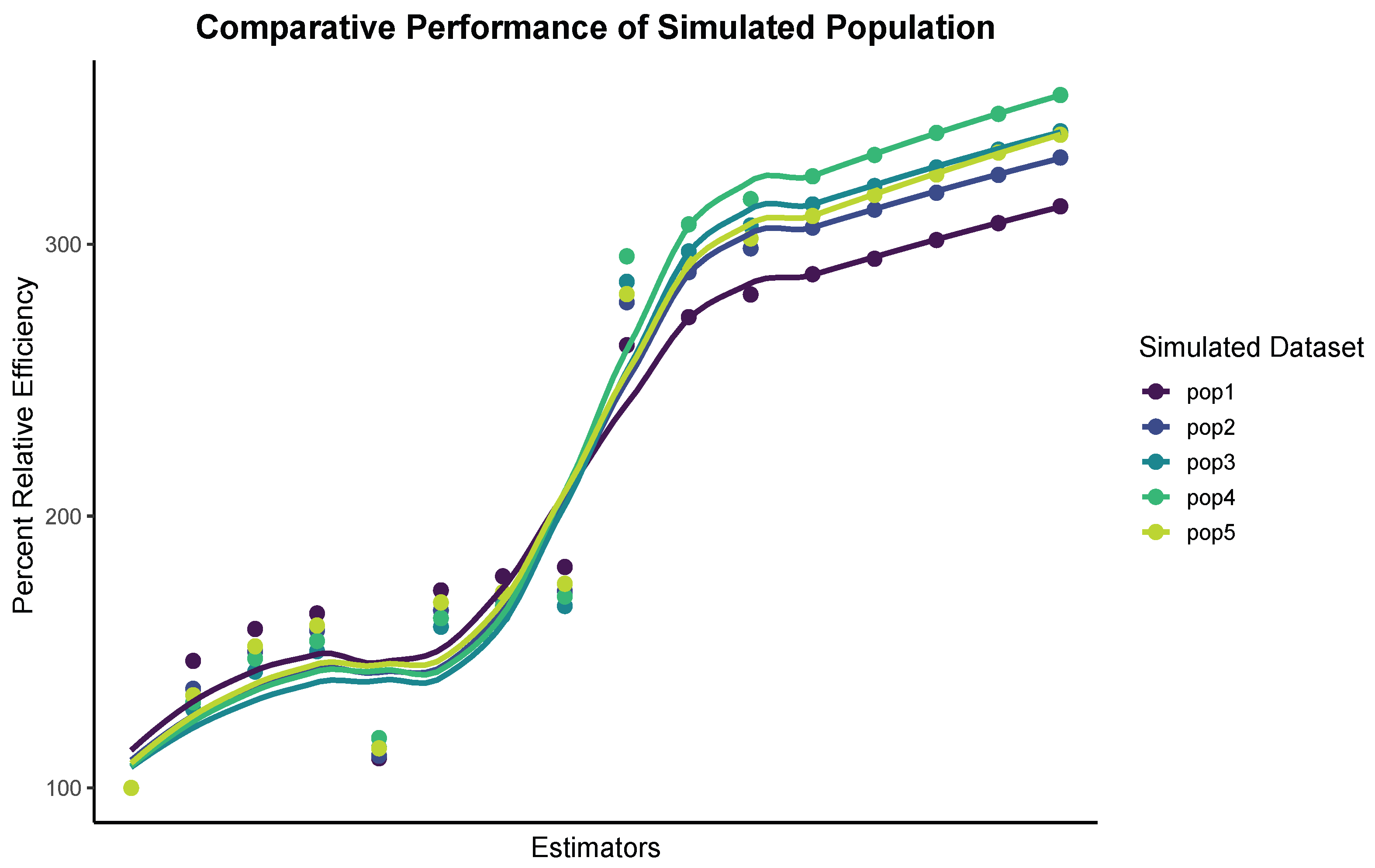
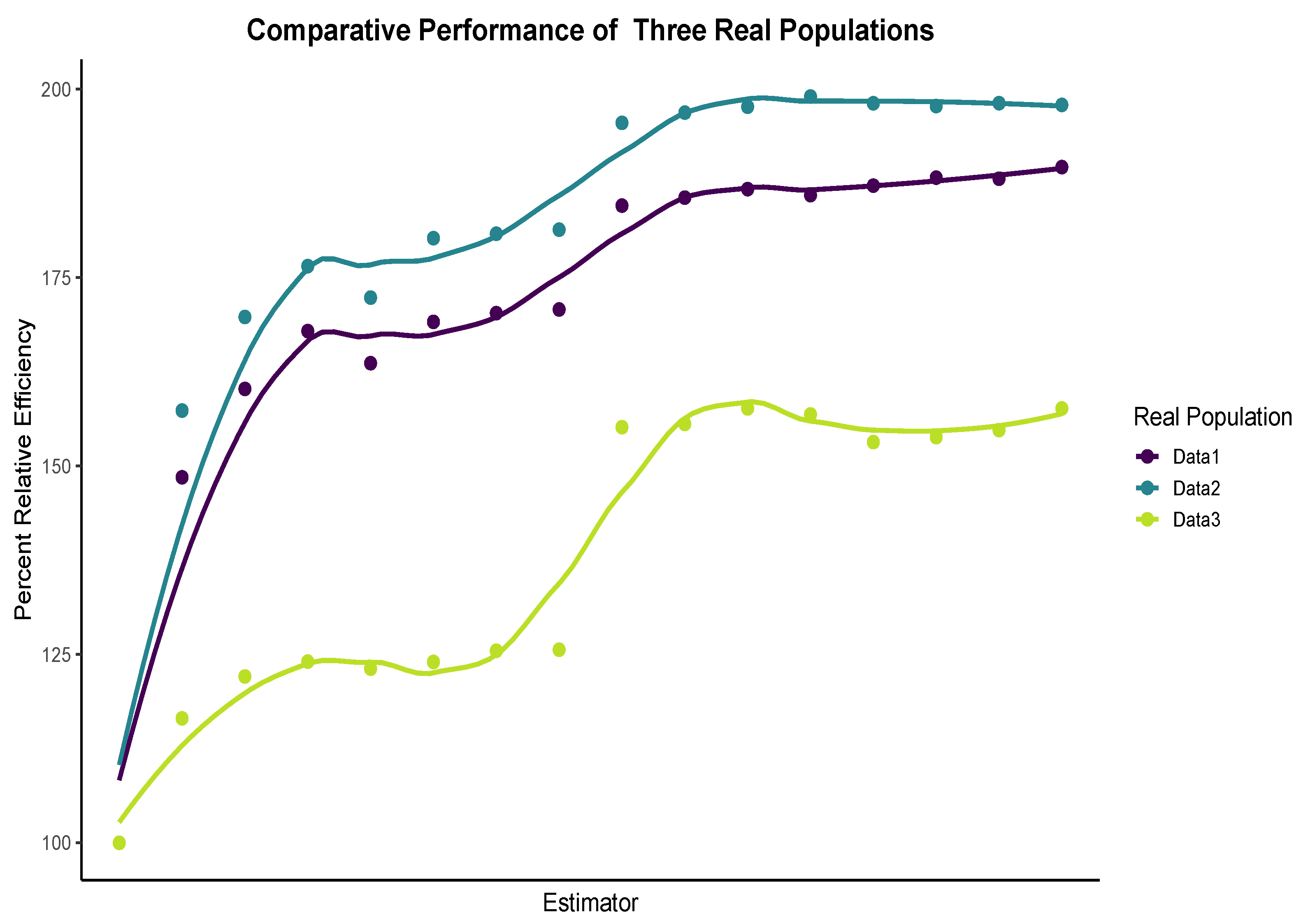
When comparing transformation-based estimators to traditional approaches, the suggested estimator class clearly outperforms traditional methods on both simulated and real-world datasets. Figure 1 and Figure 2, as well as Table 2 and

Table 6. Comparison of the PREs values based on actual population data.

Estimator	PRE-1	PRE-2	PRE-3
${\widehat{D}}_{1st}$	100.00	100.00	100.00
${\widehat{D}}_{2st}$	148.51	157.36	116.52
${\widehat{D}}_{3st}$	160.24	169.78	122.08
${\widehat{D}}_{4st}$	167.91	176.53	124.05
${\widehat{D}}_{5st}$	163.65	172.35	123.11
${\widehat{D}}_{6st}$	169.13	180.24	124.01
${\widehat{D}}_{7st}$	170.29	180.83	125.49
${\widehat{D}}_{8st}$	170.78	181.37	125.63
${\widehat{Z}}_{1st}$	184.56	195.54	155.16
${\widehat{Z}}_{2st}$	185.62	196.90	155.59
${\widehat{Z}}_{3st}$	186.74	197.68	157.65
${\widehat{Z}}_{4st}$	185.95	199.03	156.85
${\widehat{Z}}_{5st}$	187.21	198.14	153.18
${\widehat{Z}}_{6st}$	188.27	197.77	153.83
${\widehat{Z}}_{7st}$	188.13	198.15	154.77
${\widehat{Z}}_{8st}$	189.67	197.92	157.64

, provide consistent validation that the new group of estimators achieves significantly enhanced efficiency values, demonstrating their robustness in various statistical applications.

• Performance on simulated populations: All transformation-based estimators perform better than the traditional ratio, regression, exponential, and difference-type estimators across the five simulated populations, as shown in Table 2 and Figure 1. The efficiency values show a constant improvement in efficiency, as they increase gradually from $Z_{1st}$ to $Z_{8th}$. The largest PREs are recorded by estimators like $Z_{6st}$, $Z_{7st}$, and $Z_{8st}$; these estimators frequently cross 300 percent, whilst conventional estimators stay below 180 percent. This outcome highlights the significant advantages of using phase-wise stratification and auxiliary transformations, which improve stability even in distributions that are heavily tailed or strongly skewed.
• The PRE patterns observed for Populations 3 and 5 are relatively similar because both populations exhibit moderate positive correlation structures and comparatively stable distributional behavior despite originating from different distributions. In both cases, the transformation-based estimators effectively utilize auxiliary information under positively skewed population settings, resulting in closely related efficiency trends. This similarity further indicates that the proposed estimator family maintains stable performance across different distributional forms when the underlying correlation structure between the study and auxiliary variables is reasonably comparable.
• Validation on real populations: The same efficiency trends are confirmed to apply to empirical data in Table 6 and Figure 2. In all three real-life populations, the transformation-based estimators continue to produce better PRE values; the greatest overall performance is given by $Z_{8st}$. The suggested approaches show their dependability outside of controlled simulation conditions in each dataset by showing resistance to distributional asymmetry and moderate correlations between the variables Y and X.
• It is important to note that the PRE values obtained from the simulation study are comparatively larger than those observed for the real population datasets. This behavior is expected because the simulated populations were generated under controlled distributional environments specifically designed to evaluate estimator performance under skewed and heavy-tailed conditions. Under such settings, the transformation structure can more effectively utilize auxiliary information, leading to larger relative efficiency improvements.
• In contrast, real population data naturally contain additional variability arising from heterogeneous population structures, irregular correlations, measurement fluctuations, and practical survey complexities. These factors generally reduce the magnitude of achievable efficiency improvements. Nevertheless, the proposed estimators continue to demonstrate clear superiority over the existing estimators in both simulated and empirical analyses, indicating that the observed efficiency improvements are not simulation-driven but reflect the overall robustness and practical applicability of the proposed methodology.
• The derivation of the proposed estimators is based on first-order Taylor series approximation techniques commonly adopted in survey sampling theory. These approximations are developed under the assumption that the sampling errors are sufficiently small so that higher-order terms may be neglected for analytical tractability. It is acknowledged that, under extremely heavy-tailed distributions such as the Cauchy distribution, higher-order moments may not exist and the approximation accuracy may therefore be affected. However, the inclusion of the Cauchy population in the simulation study was intended to examine the practical robustness and stability of the proposed estimators under challenging distributional settings. The simulation and empirical findings indicate that the proposed estimators continue to exhibit stable and improved performance even in such heavy-tailed situations.

7. Conclusions and Future Perspectives

The study develops a transformation-based family of estimators for estimating the population median under a stratified two-phase sampling design. Analytical expressions for optimal bias and mean squared error are derived and supported by an extensive simulation study as well as real population data. The results clearly indicate that the proposed estimators consistently outperform conventional ratio, regression, difference, and exponential estimators in terms of percent relative efficiency. The improvements in efficiency are especially apparent for skewed, heavy-tailed populations or those influenced by outliers. These findings confirm that using transformations of auxiliary information under a two-phase design enhances both the stability and precision of median estimation while reducing the overall cost of data collection.

The transformation-based approach also demonstrates adaptability when the second-phase sample size is considerably smaller than that of the first phase. This property makes the estimators particularly valuable for large-scale surveys or field studies where complete auxiliary information cannot be obtained due to budgetary or logistical limitations. The ability to achieve higher precision without additional data collection enhances their appeal in socioeconomic, agricultural, and health statistics applications, where cost efficiency and robustness are equally important.

Future research may expand this framework in several meaningful directions. One promising line of inquiry is the extension of the proposed estimators to multistage and spatial sampling designs, which frequently occur in environmental and regional studies. Another important development would be to incorporate mechanisms for non-response and missing data within the same transformation structure to preserve estimator efficiency under incomplete observations. Additionally, integrating multiple auxiliary variables and exploring adaptive or nonlinear transformation functions could further enhance estimator flexibility. The inclusion of computational tools or open-source implementations would also support broader use of these methods in practice. Overall, the proposed transformation-based estimators provide a foundation for continued research on robust, cost-effective, and adaptable estimation techniques in modern survey methodology.

The simulation study is conducted under linear relationships between the study and auxiliary variables, which is a commonly adopted framework in survey sampling investigations. While the proposed estimators perform efficiently under different distributional settings, future research may further examine their behavior under nonlinear population structures and more complex dependency patterns between the study and auxiliary variables. This work mainly focuses on point estimation and efficiency improvement; however, the development of standard error estimation procedures and confidence interval methods for the proposed family of estimators may further improve its practical applicability. Therefore, future research may focus on inferential procedures and interval estimation under stratified two-phase sampling schemes.

References

1. Cochran, W.B. Sampling Techniques; John Wiley and Sons: Hoboken, NJ, USA, 1963. [Google Scholar]
2. Särndal, C.E. Sample survey theory vs. general statistical theory: Estimation of the population mean. Int. Stat. Rev./Rev. Int. Stat. 1972, 40, 1–12. [Google Scholar] [CrossRef]
3. Stigler, S.M. Linear functions of order statistics. Ann. Math. Stat. 1969, 40, 770–788. [Google Scholar] [CrossRef]
4. Gross, S. Median estimation in sample surveys. In Proceedings of the Section on Survey Research Methods; American Statistical Association Ithaca: Alexandria, VA, USA, 1980. [Google Scholar]
5. Sedransk, J.; Meyer, J. Confidence intervals for the quantiles of a finite population: Simple random and stratified simple random sampling. J. R. Stat. Soc. Ser. B (Methodol.) 1978, 40, 239–252. [Google Scholar] [CrossRef]
6. Philip, S.; Sedransk, J. Lower bounds for confidence coefficients for confidence intervals for finite population quantiles. Commun. Stat.-Theory Methods 1983, 12, 1329–1344. [Google Scholar] [CrossRef]
7. Kuk, Y.C.A.; Mak, T.K. Median estimation in the presence of auxiliary information. J. R. Stat. Soc. Ser. B 1989, 51, 261–269. [Google Scholar] [CrossRef]
8. Rao, T.J. On certail methods of improving ration and regression estimators. Commun. Stat.-Theory Methods 1991, 20, 3325–3340. [Google Scholar] [CrossRef]
9. Singh, S.; Joarder, A.H.; Tracy, D.S. Median estimation using double sampling. Aust. N. Z. J. Stat. 2001, 43, 33–46. [Google Scholar] [CrossRef]
10. Khoshnevisan, M.; Singh, H.P.; Singh, S.; Smarandache, F. A General Class of Estimators of Population Median Using Two Auxiliary Variables in Double Sampling; Virginia Polytechnic Institute and State University: Blacksburg, VA, USA, 2002. [Google Scholar]
11. Singh, S. Advanced Sampling Theory with Applications: How Michael Selected Amy; Springer Science & Business Media: Berlin/Heidelberg, Germany, 2003; Volume 2. [Google Scholar]
12. Gupta, S.; Shabbir, J.; Ahmad, S. Estimation of median in two-phase sampling using two auxiliary variables. Commun. Stat.-Theory Methods 2008, 37, 1815–1822. [Google Scholar] [CrossRef]
13. Aladag, S.; Cingi, H. Improvement in estimating the population median in simple random sampling and stratified random sampling using auxiliary information. Commun. Stat.-Theory Methods 2015, 44, 1013–1032. [Google Scholar] [CrossRef]
14. Solanki, R.S.; Singh, H.P. Some classes of estimators for median estimation in survey sampling. Commun. Stat.-Theory Methods 2015, 44, 1450–1465. [Google Scholar] [CrossRef]
15. Daraz, U.; Almulhim, F.A.; Alomair, M.A.; Alomair, A.M. Population median estimation using auxiliary variables: A simulation study with real data across sample sizes and parameters. Mathematics 2025, 13, 1660. [Google Scholar] [CrossRef]
16. Sharma, P.; Lata, A.; Yadav, S.K.; Noor-ul-Amin, M. Family of estimators for estimating population median using auxiliary information in survey sampling. J. Reliab. Stat. Stud. 2025, 18, 343–370. [Google Scholar] [CrossRef]
17. Baig, A.; Masood, S.; Ahmed Tarray, T. Improved class of difference-type estimators for population median in survey sampling. Commun. Stat.-Theory Methods 2019, 49, 5778–5793. [Google Scholar] [CrossRef]
18. Sharma, P.; Singh, R. Generalized class of estimators for population median using auxiliary information. Hacet. J. Math. Stat. 2015, 44, 443–453. [Google Scholar] [CrossRef]
19. Masood, S.; Ibrar, B.; Shabbir, J.; Movaheedil, Z. Estimating neutrosophic finite median employing robust measures of the auxiliary variable. Sci. Rep. 2024, 14, 10255. [Google Scholar] [CrossRef] [PubMed]
20. Sharma, P.; Pusa, N.; Kumari, M.; Singh, P. Balancing accuracy and cost: A new estimator for stratified random sampling. Commun. Stat.-Simul. Comput. 2025, 1–17. [Google Scholar] [CrossRef]
21. Shabbir, J.; Gupta, S. A generalized class of difference type estimators for population median in survey sampling. Hacet. J. Math. Stat. 2017, 46, 1015–1028. [Google Scholar] [CrossRef]
22. Irfan, M.; Maria, J.; Shongwe, S.C.; Zohaib, M.; Bhatti, S.H. Estimation of population median under robust measures of an auxiliary variable. Math. Probl. Eng. 2021, 2021, 4839077. [Google Scholar] [CrossRef]
23. Shabbir, J.; Gupta, S.; Narjis, G. On improved class of difference type estimators for population median in survey sampling. Commun. Stat.-Theory Methods 2022, 51, 3334–3354. [Google Scholar] [CrossRef]
24. Subzar, M.; Lone, S.A.; Ekpenyong, E.J.; Salam, A.; Aslam, M.; Raja, T.A.; Almutlak, S.A. Efficient class of ratio cum median estimators for estimating the population median. PLoS ONE 2023, 18, e0274690. [Google Scholar] [CrossRef] [PubMed]
25. Iseh, M.J. Model formulation on efficiency for median estimation under a fixed cost in survey sampling. Model Assist. Stat. Appl. 2023, 18, 373–385. [Google Scholar] [CrossRef]
26. Alghamdi, A.S.; Almulhim, F.A. Stratified median estimation using auxiliary transformations: A robust and efficient approach in asymmetric populations. Axioms 2025, 17, 1127. [Google Scholar] [CrossRef]
27. Singh, H.P.; Vishwakarma, G.K. Modified exponential ratio and product estimators for finite population mean in double sampling. Austrian J. Stat. 2007, 36, 217–225. [Google Scholar] [CrossRef]
28. Bureau of Statistics. Punjab Development Statistics Government of the Punjab, Lahore, Pakistan; Bureau of Statistics: Islamabad, Pakistan, 2013. [Google Scholar]
29. Bureau of Statistics. Punjab Development Statistics Government of the Punjab, Lahore, Pakistan; Bureau of Statistics: Islamabad, Pakistan, 2014. [Google Scholar]
Figure 1. The graph shows how well the new class of estimators works compared to the previous ones by showing their percent relative efficiency on simulated data.
Symmetry 18 00933 g001
Figure 2. The graph compares the efficiency of a new group of estimators and previous estimators through their PRE on real data.
Symmetry 18 00933 g002