4.1. Datasets and Data Preparation
Experiments are conducted on the public CALCE A123 battery dataset, as introduced in Ref. [
44]. This dataset has been widely adopted in battery modeling and SOC estimation studies because it provides carefully curated cycling records with synchronized voltage, current, and temperature measurements, together with dynamic load profiles that are close to electric-vehicle operating scenarios [
45]. In the present work, CALCE is used to evaluate estimation accuracy under different fixed ambient temperatures and operating conditions within a consistent dynamic-drive-cycle setting.
For the CALCE benchmark, this study focuses on the A123 lithium-ion cells tested under dynamic driving-related current profiles. The CALCE dynamic dataset contains three representative operating conditions, namely the Federal Urban Driving Schedule (FUDS), Dynamic Stress Test (DST), and US06 highway driving profile [
44]. Among them, FUDS is selected as the primary operating condition for the main comparison experiments. The reason is twofold. First, FUDS describes typical urban electric-vehicle driving behavior, including start-up, acceleration, cruising, deceleration, and stop phases, and is therefore more representative of practical battery-management scenarios than a purely simplified laboratory load. Second, compared with DST, which is derived from a simplified power–time profile, and US06, which emphasizes more aggressive high-speed and high-acceleration operation, FUDS provides a better balance between dynamic richness and practical relevance. Unless otherwise specified, the main experimental setting in this paper is the CALCE A123 dataset under the FUDS profile at 25 °C. In addition, performance under different fixed ambient temperatures is evaluated under 0 °C, 10 °C, 25 °C, and 40 °C, while DST and US06 are retained as supplementary operating conditions for condition-wise comparison.
To examine whether the proposed framework generalizes beyond the original CALCE A123 benchmark, external validation is conducted on the NASA Ames lithium-ion battery aging dataset [
46]. Four commonly used laboratory-scale 18650 cells, B0005, B0006, B0007, and B0018, are selected because they provide synchronized voltage, current, measured cell temperature, time, and discharge-capacity records over repeated cycling. In the NASA experiment, SOC labels are generated from the discharge trajectories by the same Coulomb-counting protocol, and a leave-one-cell-out strategy is adopted: one cell is used only for testing, while the remaining three cells are used for training and validation. This protocol evaluates cell-level generalization under an independent public benchmark rather than random sample-level interpolation within a single cell. The NASA dataset is used here as a classical external benchmark and should not be interpreted as a modern high-capacity NMC/NCA EV-pack dataset.
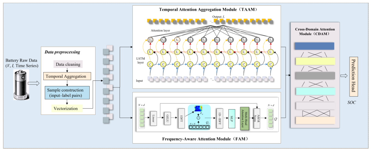
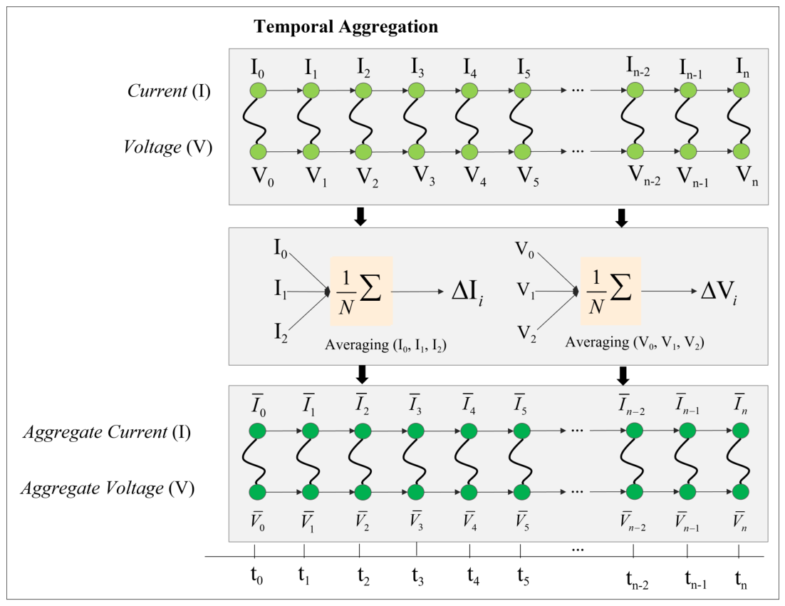
To ensure consistency with the proposed JTFCD-Net, raw measurements are processed under a unified pipeline. First, only complete discharge trajectories containing valid voltage, current, and temperature measurements are retained. Since the present work focuses on SOC estimation together with voltage reconstruction during dynamic evolution, sliding windows are sampled from these discharge trajectories for training and testing. For the main comparative experiments, FUDS discharge trajectories at the selected temperatures are used; DST and US06 are included in the operating-condition study. Second, duplicated timestamps, missing samples, and obvious outliers are removed, after which the remaining trajectories are resampled to a uniform time interval using linear interpolation. This step is necessary because both the dual-task learning target and the temporal modules in JTFCD-Net assume a consistent temporal grid.
The reference SOC labels are generated by Coulomb counting. Let
denote the discharge current magnitude at time step
t and
denote the reference capacity used for label construction. The discrete reference SOC label is computed as
where
is the Coulombic efficiency and the initial SOC of each selected discharge trajectory is set to
. In the present CALCE study, a unified
and constant
are adopted for all selected trajectories to keep the label construction protocol consistent across the dataset and all compared models. Therefore, these SOC values are treated as Coulomb-counting-based reference labels rather than error-free physical ground truths.
After label generation, each time step is represented by a multivariate feature vector
where
The inclusion of both raw measurements and first-order temporal differences is designed to match the temporal aggregation block introduced in
Section 3.2. Specifically, the multi-branch one-dimensional convolutions in the temporal aggregation module are intended to capture local transients at different receptive fields. The raw channels provide absolute operating-state information, whereas the differential channels explicitly highlight local voltage and current transitions, enabling the convolution branches to respond more effectively to abrupt load perturbations, relaxation behavior, and local trend changes. It should also be noted that first-order differencing may amplify measurement noise, especially under real dynamic driving conditions with imperfect onboard sensors. In this study, this risk is partly mitigated by removing missing samples and obvious outliers, resampling all trajectories to a uniform time grid, normalizing each feature channel using training-set statistics, and processing the resulting features through fixed-length sliding windows with multi-scale convolution and attention-based aggregation. Nevertheless, these operations should be viewed as noise-mitigation measures rather than a complete solution to sensor-noise robustness.
All feature channels are normalized using statistics computed from the training set only:
where
and
denote the mean and standard deviation of the
j-th feature channel. Sliding windows are then constructed to form the model input:
where
in the present implementation. For each input window, the supervision signals are the terminal SOC label
and the voltage reconstruction target
In this manner, the dataset construction process is fully aligned with the dual-task design of JTFCD-Net. The fixed-length input tensor preserves the local neighborhoods required by temporal aggregation, while the full window voltage target supplies the sequence-level supervision used by the reconstruction branch. This auxiliary target is important because SOC supervision alone is sparse at the window level, whereas reconstructing encourages the shared backbone to preserve the temporal morphology of battery response, including transient drops, recovery effects, and temperature-dependent polarization behavior. In this paper, the role of the voltage branch is to improve the reliability of SOC estimation by helping the backbone retain informative intermediate dynamics that would otherwise be compressed away when optimizing only the terminal SOC target.
To avoid information leakage, the trajectories of each battery cell are divided in chronological order with a ratio of 70% for training, 15% for validation, and 15% for testing. The earlier portion is used for training, the middle portion for validation, and the later portion for testing, so that the model is always evaluated on later operating stages that are unseen during optimization. All sliding windows inherit the split of the parent trajectory.
4.3. Experimental Settings
The proposed JTFCD-Net is implemented in PyTorch 2.0.1 and trained end-to-end on a single GPU platform. Unless otherwise stated, the window length is set to , the hidden feature dimension is set to , the number of attention heads in TAAM is , and the shared cross-domain attention dimension in CDAM is set to . In the temporal aggregation block, three parallel one-dimensional convolution branches are employed with kernel sizes to capture local battery dynamics at different temporal scales. For the feed-forward block in TAAM, the intermediate dimension is set to . In FAM, the channel reduction dimension is set to . The loss balancing coefficient in the joint objective is fixed to .
During training, the Adam optimizer is adopted with an initial learning rate of , a batch size of 128, and a weight decay of . The model is trained for at most 200 epochs, and early stopping is applied according to the validation RMSE to avoid overfitting. The learning rate is reduced automatically when the validation performance saturates. All input normalization statistics are computed only from the training split, and the same normalization parameters are reused for validation and test samples to ensure a fair evaluation protocol.
All compared methods use the same data split and the same input variables whenever possible. The optimizer family, epoch budget, early-stopping criterion, and normalization protocol are kept consistent across methods. This setting helps ensure that the reported performance differences mainly reflect differences in representation learning and supervision design rather than inconsistencies in data partitioning or preprocessing. Under this protocol, the proposed JTFCD-Net can be evaluated consistently on CALCE while maintaining alignment between the dataset construction procedure and the architecture described in
Section 3.
4.4. Computational Complexity and Inference Cost
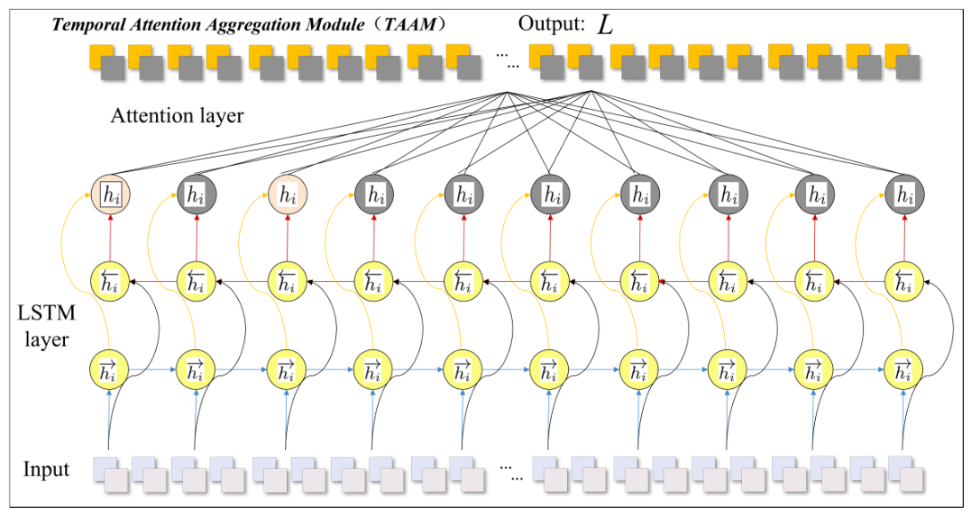
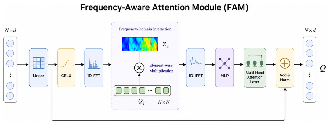
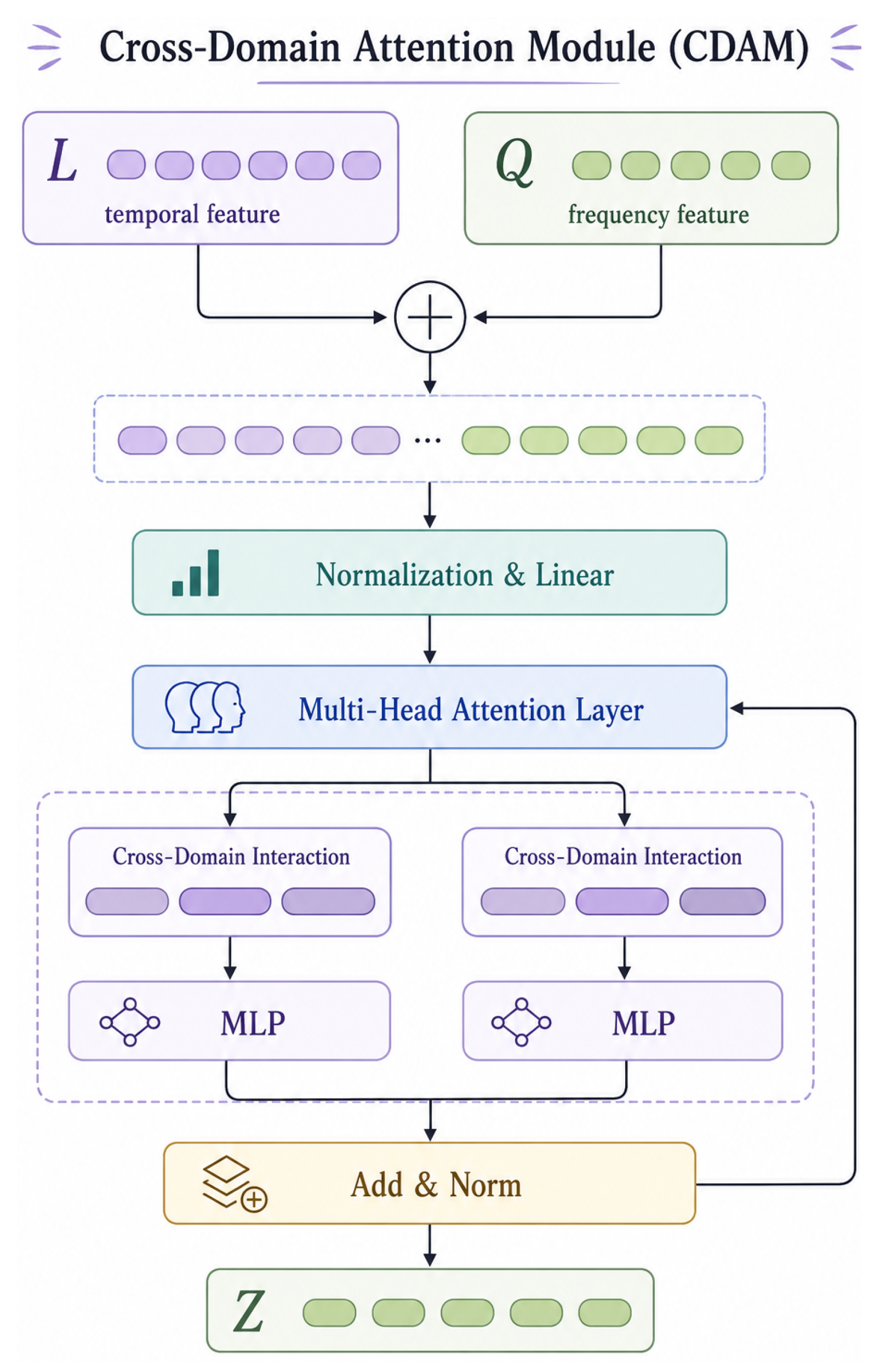
The computational cost of JTFCD-Net is mainly determined by the multi-scale temporal aggregation block, TAAM, FAM, and CDAM. For a window length L, input dimension , hidden dimension d, feed-forward dimension , CDAM projection dimension , and FAM reduction dimension r, the temporal aggregation block costs approximately . TAAM costs , where the term comes from temporal self-attention. FAM costs because it uses one global Fourier transform and a small channel MLP. CDAM costs and stores two attention matrices. Therefore, TAAM and CDAM dominate the total complexity, while FAM contributes only a small additional cost.
Under the default setting used in this study (, , , , and ), the implemented JTFCD-Net contains approximately trainable parameters (0.24 M). Single-window inference was profiled with batch size 1 and on the CPU of the same workstation used for experiments, giving an average latency of about ms per window. This result provides a practical reference for the implemented model size and workstation-level inference cost.
4.5. Baseline Models
To verify the effectiveness of the proposed backbone, JTFCD-Net is compared with six representative sequence modeling baselines, including a vanilla recurrent neural network (RNN), LSTM, BiLSTM, 1D-CNN, Transformer, and Mamba. These baselines cover the main families of sequence processing methods that are widely used in time-series learning and battery state estimation, namely plain recurrent modeling [
40,
47], gated recurrence [
17,
48], bidirectional recurrence [
23,
49], convolutional sequence encoding [
21,
50], self-attention [
31,
51], and state-space sequence modeling [
52]. The inclusion of these methods allows the comparison to cover both classical and recent long-sequence architectures under a unified SOC estimation protocol.
For fairness, all baseline models use the same sliding-window input, the same normalized feature channels, the same train–validation–test split, and the same optimizer family and training schedule described in
Section 4.3. The hidden width and number of layers of each baseline are adjusted so that the trainable parameter budgets are kept in the same sub-million scale as JTFCD-Net. The parameter counts reported in
Table 1 are rounded implementation-level estimates, including the prediction head, and are used only to indicate model-scale comparability rather than exact framework-independent constants. Unless otherwise stated, recurrent baselines use the final hidden state for SOC regression, whereas 1D-CNN, Transformer, and Mamba apply temporal average pooling followed by the same two-layer multilayer perceptron prediction head. The references associated with each baseline are intended to indicate the original or representative source of the corresponding model family; the baselines used here are standardized implementations under a unified protocol rather than exact reproductions of every published training protocol.
CNN–LSTM [
19], a representative hybrid architecture that combines local convolutional feature extraction with recurrent temporal modeling, is included in the main CALCE benchmark. In the NASA external validation, JTFCD-Net is compared with Mamba, which is the strongest baseline in the CALCE experiments, and CNN–LSTM as a hybrid baseline. A full physics-informed-neural-network comparison is not included in the current experimental scope because such models typically require additional physical assumptions, equivalent-circuit identification, or electrochemical parameters that are not uniformly specified in the selected public datasets.
4.6. Comparison with Baseline Methods
Based on the above settings, several groups of comparative experiments are conducted. Unless otherwise specified, the main comparison setting is the CALCE A123 dataset under the FUDS operating profile at 25 °C. On top of this main benchmark, analyses are performed to study performance under different fixed ambient temperatures for FUDS and operating-condition robustness under DST and US06. Following common practice in the battery estimation literature, all SOC errors are multiplied by 100 and reported in percentage form. All external baseline methods are trained using SOC supervision only, and JTFCD-Net (SOC-only) is also reported by setting
. The full JTFCD-Net is trained with the joint SOC estimation and voltage reconstruction objective described in
Section 3. This difference in supervision is intentional: the auxiliary voltage branch is part of the proposed method itself and is introduced to improve the reliability of SOC estimation under dynamic conditions. Therefore, the comparison should be interpreted as an overall framework comparison under matched data splits, inputs, and model scale, rather than as a same-supervision ablation of backbone architectures. In all tables, the model names are followed by their representative source references. The architecture ablation studies are conducted under the main setting of CALCE FUDS at 25 °C, while a temperature-input ablation is included in the NASA external validation. This ablation evaluates the use of measured cell-temperature information, not robustness under prescribed pack-level dynamic thermal profiles.
Several observations can be drawn from
Table 2,
Table 3 and
Table 4. First, under the main comparison setting of CALCE FUDS at 25 °C, JTFCD-Net yields the lowest errors, with an MAE of 0.11%, an RMSE of 0.15%, and a MaxE of 0.47%. The CNN–LSTM baseline obtains an RMSE of 0.24%, which is better than the standalone LSTM and 1D-CNN baselines but still weaker than the stronger global-sequence baselines and the proposed method. The SOC-only variant still outperforms the strongest external baseline, while full voltage reconstruction further reduces the RMSE from 0.18% to 0.15%. The improvement over Mamba and Transformer is clear but still moderate, which better reflects a realistic advantage under a strong baseline setting rather than an excessively optimistic gap. Compared with Mamba, the absolute MAE reduction is only 0.04 percentage points, so the engineering impact should be interpreted as incremental rather than decisive.
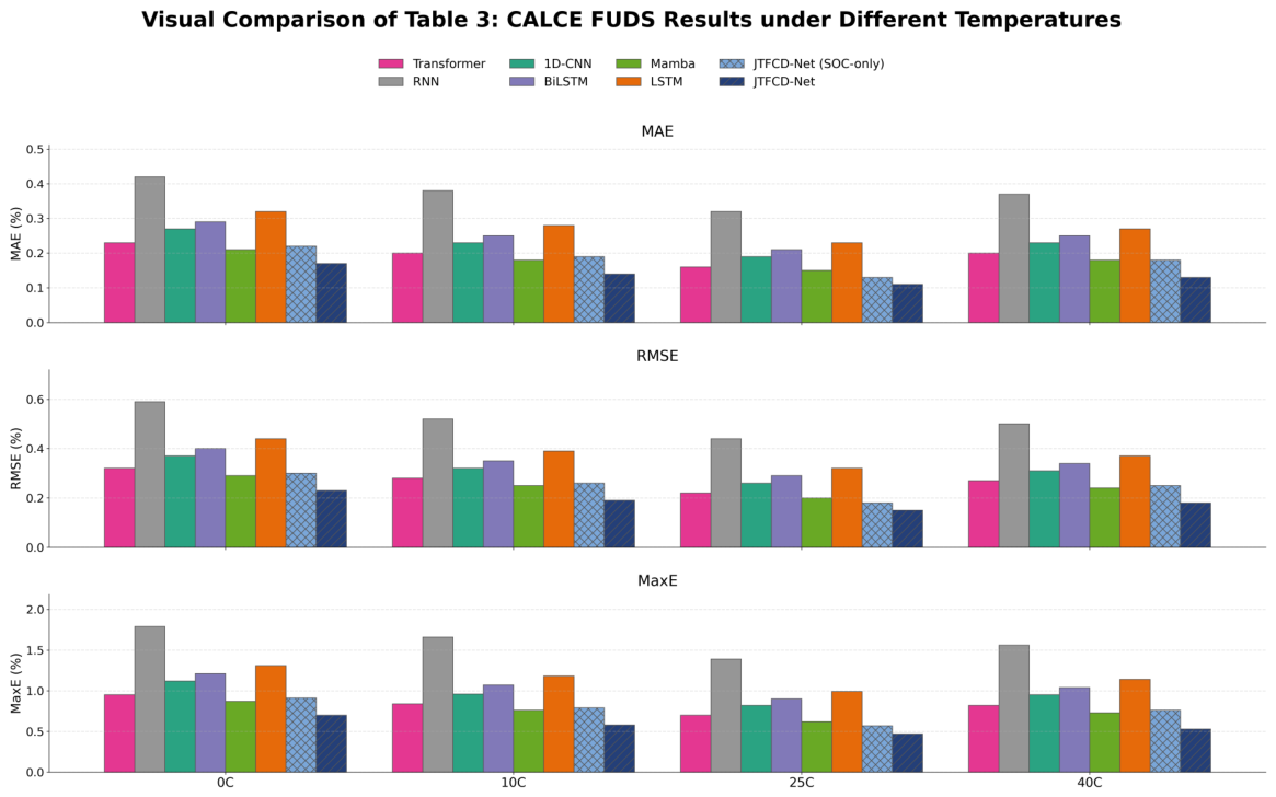
Second, the CALCE FUDS fixed-temperature comparison results show a clear thermal effect. The most challenging case is 0 °C, where all models exhibit their largest errors. This behavior is physically reasonable because low temperature increases polarization, internal resistance, and voltage hysteresis, making the mapping from measurable terminal signals to latent SOC more nonlinear and less stable. As the temperature approaches 25 °C, the error of every method decreases, which indicates that the electrochemical response becomes easier to model under moderate thermal conditions. At 40 °C, the error rises slightly again, reflecting the influence of temperature-induced side reactions and drift in dynamic behavior. The SOC-only variant is not consistently better than Mamba under all temperatures, whereas the full model remains clearly better after adding voltage reconstruction supervision. However, these controlled isothermal tests should not be interpreted as direct evidence of robustness under continuously varying pack-temperature trajectories during real vehicle operation.
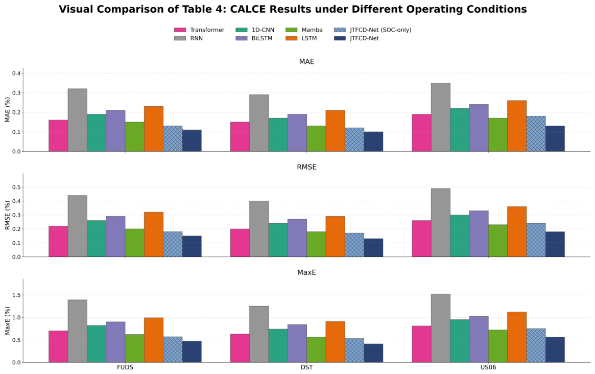
Third, the supplementary CALCE condition comparison demonstrates that the proposed method is not limited to FUDS alone. At 25 °C, JTFCD-Net attains the lowest MAE, RMSE, and MaxE under FUDS, DST, and US06. Among the three conditions, DST is slightly easier because its load profile is more regular, whereas US06 is the most challenging because it contains more aggressive high-power transients. Under US06, JTFCD-Net (SOC-only) is slightly weaker than Mamba, indicating that the auxiliary task is especially useful under aggressive load variation. This pattern is consistent with the design motivation of the temporal and frequency branches: multi-scale local aggregation helps capture rapid current changes, while TAAM, FAM, and CDAM help maintain stable estimation under more abrupt and spectrally complex load profiles.
Fourth, the relative ranking of the baseline models is also informative. The gated recurrent baselines outperform the vanilla RNN, confirming that long-term memory is essential for battery SOC tracking. The 1D-CNN baseline further improves over recurrent models because local transients and short-term voltage-current interactions are important in dynamic SOC estimation. Transformer and Mamba provide stronger performance than the purely recurrent and convolutional baselines, indicating that global dependency modeling is beneficial. Nevertheless, their improvements remain limited compared with JTFCD-Net because they do not explicitly combine multi-scale temporal aggregation, frequency-informed channel recalibration, and cross-domain fusion under a dual-task learning objective.
For clearer interpretation of the numerical results, the data reported in
Table 3 and
Table 4 are further visualized in grouped bar charts, as shown in
Figure 6 and
Figure 7. The visual comparison makes the relative margin among competing methods more intuitive. In particular, the advantage of JTFCD-Net can be observed consistently across all three error metrics, and the margin becomes more pronounced under low-temperature or highly dynamic conditions. This performance pattern is consistent with representation-level temporal–frequency symmetry, which incorporates complementary frequency-aware cues into temporal representations.
4.9. Ablation Studies
To analyze the contribution of each design component, a series of ablation experiments are conducted only under the main experimental setting of CALCE FUDS at 25 °C. The ablations focus on five aspects: backbone module contribution, the role of voltage reconstruction supervision, the effect of multi-scale temporal aggregation, the effect of observation window length, and the sensitivity to the loss balancing coefficient. Unless otherwise stated, the ablation experiments follow the same training settings as the full model.
To justify the default choice of
, a sensitivity analysis is conducted by changing only the observation window length while keeping the remaining model and training settings unchanged. As shown in
Table 8, increasing
L from 64 to 128 clearly reduces SOC RMSE, whereas further increasing
L to 256 provides only a slight improvement from 0.15% to 0.14%. In contrast, the relative theoretical cost, computed from the complexity terms in
Section 4.4 and normalized to
, increases to about
at
. Therefore,
is selected as a balanced setting between estimation accuracy and computational overhead.
Several conclusions can be drawn from the ablation results. First,
Table 9 shows that each proposed module contributes positively to performance under the main benchmark of CALCE FUDS at 25 °C. TAAM provides a substantial improvement over the temporal aggregation front end alone, indicating the importance of long-range dependency modeling. The band-aware FAM variant improves only slightly over TAAM, whereas the proposed FAM yields a larger gain, suggesting that lightweight global spectral channel recalibration is more effective in this setting than explicit band splitting. This ablation compares end-to-end frequency modeling variants within the same backbone, not all handcrafted spectral augmentations. Replacing simple concatenation with CDAM further reduces RMSE from 0.20% to 0.18%, but this improvement is moderate rather than decisive; therefore, CDAM should be viewed as an explicit interaction design whose cost–benefit trade-off requires careful consideration for real-time deployment. The best results are obtained only when all modules are retained and jointly optimized.
Second,
Table 10 directly verifies the importance of voltage reconstruction supervision. When the auxiliary branch is removed, the SOC RMSE increases from 0.15% to 0.18%. Replacing full-window voltage reconstruction with only a terminal-voltage target provides limited benefit, but it still remains inferior to reconstructing the entire voltage sequence. This result supports the central design choice of the paper: dense sequence-level voltage supervision helps preserve informative intermediate dynamics and thereby improves the reliability of SOC estimation more effectively than a point-wise auxiliary target.
Third,
Table 11 shows that the multi-scale temporal aggregation strategy is consistently better than any single receptive field. This observation is physically intuitive because battery voltage response contains short-term current-induced drops, medium-term polarization effects, and slower recovery components. A single convolution kernel cannot capture all these dynamics equally well, whereas the proposed multi-branch design provides a more complete local description before the sequence is processed by the later attention and cross-domain modules.
Fourth,
Table 8 shows that the default window length is a practical compromise. The shorter window
reduces cost but loses useful temporal context, while
yields only marginal accuracy improvement at substantially higher computational cost.
Finally,
Table 12 shows that the tradeoff coefficient
should remain moderate. When
is too small, the auxiliary branch cannot contribute enough reliability-enhancing supervision; when it is too large, the optimization focus shifts excessively toward voltage reconstruction. The best balance is achieved at
, which is therefore adopted in all main experiments.