Damage Imaging in Plate Structures Under Broadband Chirp Excitation Based on f-k Domain Modal Separation and Additive–Multiplicative Modal Fusion

Abstract

Compared with conventional narrowband excitation, broadband chirp excitation covers a wider frequency range and can therefore provide richer damage-response information for plate structures. In this study, the application of a modal superposition imaging method based on frequency-wavenumber (f-k) domain modal separation and additive–multiplicative fusion under broadband chirp excitation was investigated through numerical simulations and experiments. First, the acquired signals were separated in the f-k domain, and the A₀ and S₀ modal responses were extracted, respectively. Subsequently, modal fusion imaging was implemented by fusing the imaging results of different modes through additive–multiplicative modal fusion. The results show that, within the selected frequency band, single-modal imaging can effectively characterize the damage location, whereas modal fusion can further reduce the damage region and improve the localization accuracy. Compared with time-domain common-source method (CSM) imaging, the f-k domain method can make fuller use of the effective frequency components within the selected frequency band and can account for guided-wave dispersion, thereby producing more compact imaging results while maintaining localization accuracy. These results verify the effectiveness of the proposed method under broadband chirp excitation and demonstrate its potential for multimodal damage identification.

1. Introduction

Traditionally, the excitation signals used for guided-wave-based damage detection in plate structures are narrowband sinusoidal waves modulated by window functions. Their narrow bandwidth suppresses dispersion to the greatest extent and generates single-mode guided waves with relatively weak dispersive effects [1]. However, narrowband signals cannot cover all characteristic frequencies associated with damage and can provide only partial damage-related information, thereby limiting the evaluation accuracy of modal-analysis-based methods. In addition, related theoretical studies on nonlinear evolution equations have also enriched the understanding of complex wave-propagation and dispersion phenomena [2]. For this reason, linear chirp excitation has attracted increasing attention in guided-wave inspection in recent years [3,4]. Because its instantaneous frequency continuously sweeps over a prescribed range, a chirp signal can cover the entire frequency band and is therefore suitable for frequency-sweep testing as well as multiband and multimodal detection [5,6]. In 2013, Michaels et al. [7] demonstrated the use of broadband chirp excitation to generate ultrasonic guided waves in plate structures, showing that chirp signals can efficiently excite Lamb waves across a wide frequency range with improved data acquisition efficiency and signal-to-noise characteristics. In 2018, Feng et al. [8] applied chirp-excited Lamb waves to damage detection in composite plates and demonstrated their effectiveness for delamination identification in anisotropic carbon-fiber-reinforced polymer (CFRP) structures. In 2022, Tan et al. [9] pointed out that broadband chirp excitation can cover multiple frequency responses within a single excitation, enabling the simultaneous acquisition of multimodal information, reducing repeated excitation, and improving detection efficiency. In 2023, Xu et al. [10] combined nonlinear chirp signals with a pulse-compression method to achieve high-contrast imaging under low excitation amplitudes while obtaining damage-sensitive features at multiple frequencies. In 2025, Li et al. [11] further proposed a full-focusing imaging method that exploits the full-frequency contribution of broadband guided-wave echoes, effectively improving spatial resolution and imaging accuracy in plate structures. These studies indicate that broadband chirp excitation can acquire rich multi-frequency and multimodal information, thereby providing comprehensive signal features for damage imaging. However, when such multi-frequency and multimodal signals are directly used for imaging, noise, modal aliasing, and dispersion may reduce imaging quality, and their advantages cannot be fully exploited. Therefore, the effective integration of multi-frequency and multimodal information has become a key issue in further improving the accuracy of damage imaging in plate structures.

In recent years, multisource data-fusion methods have been widely applied to damage detection and imaging so as to fully exploit information from different sensors, frequencies, and modes, thereby improving the accuracy and robustness of damage identification [12,13,14,15]. In 2016, He et al. [16] employed single-mode reverse-time migration and a normalized zero-lag cross-correlation imaging condition to image and quantitatively analyze multiple damages in isotropic plates. In 2018, Chang et al. [17] proposed a matrix beamforming method using a linear chirp signal as the excitation source and a scanning laser Doppler vibrometer (SLDV) as the receiver to measure guided-wave fields in thick aluminum and composite plates. In 2022, Guo et al. [18] adopted a probabilistic imaging method in composite structures to statistically fuse multichannel sensor data, thereby achieving high-precision localization and quantitative analysis of slight damage. In 2023, Xu et al. [19] proposed a multi-narrowband frequency-fusion strategy for phased-array imaging, in which Lamb-wave signals at different frequencies were combined in a weighted manner, effectively suppressing sidelobe interference and improving the spatial resolution of damage localization. In 2024, Zhang et al. [20] combined Lamb waves with a Bayesian fusion algorithm and integrated signal information from different paths through a probabilistic model, thereby achieving high-precision damage-localization imaging while reducing dependence on the number of sensors. In addition, Yang et al. [21] proposed a decision-level sensor-fusion method that jointly used guided-wave monitoring data and vibration-sensor data, thereby enhancing damage discrimination and localization stability through decision-level integration. In 2025, Gao et al. [22] further proposed a dual-frequency fusion method. By combining imaging results at two different frequencies, the grating-lobe effect was significantly reduced, and imaging clarity and localization accuracy were improved. In the same year, Zhu et al. [23] also excited different modal signals using broadband excitation and demonstrated that broadband excitation after multiband filtering yields better structural damage imaging than narrowband excitation. These studies show that, through appropriate data-fusion strategies, information from different sources can complement one another, which not only improves the accuracy of single-sensor or single-frequency imaging, but also significantly enhances damage localization and imaging performance in structures [24,25]. Although these studies have provided an important foundation for broadband guided-wave imaging and multimodal fusion, some limitations still remain. First, although broadband chirp excitation can provide rich multifrequency and multimodal information within a single excitation, if it is directly used for imaging, it is still susceptible to dispersion, modal aliasing, and redundant reflected components, making it difficult for the advantages of broadband information to be fully utilized. Second, existing fusion studies have mainly focused on multifrequency information fusion, multi-sensor fusion, or modal information utilization at a single level, whereas studies on combining modal separation with modal fusion imaging under broadband conditions remain relatively limited. Therefore, under broadband chirp excitation, how to effectively separate multimodal guided-wave responses, fully utilize the effective frequency-segmented information within the selected band, and improve the accuracy of damage localization and imaging through appropriate modal fusion remains a key issue that deserves further investigation.

To address the above issues, a broadband guided-wave damage-imaging method based on f-k domain modal separation and additive–multiplicative modal fusion is proposed in this study. Unlike approaches in which broadband responses are approximated as single-center-frequency signals, the broadband chirp response is regarded herein as being composed of multiple frequency-segmented components, so that damage-sensitive information within the selected frequency band can be more fully retained while guided-wave dispersion is taken into account. On this basis, the A₀ and S₀ low-order modes are explicitly separated in the f-k domain, and time-domain common-source method (CSM) imaging and f-k domain CSM imaging are performed, respectively, under the same broadband multimodal condition, so that a direct comparison between the two imaging routes can be achieved. Furthermore, an additive–multiplicative modal fusion strategy is adopted to fuse the imaging results of different modes, so that the damage region jointly indicated by different modes can be highlighted while mode-specific background spurious responses can be suppressed. Through finite element simulations and experimental validation, the localization accuracy, image compactness, and applicability of the proposed method in broadband guided-wave damage imaging of plate structures were systematically investigated in this study, thereby providing a new approach for multimodal guided-wave damage imaging under broadband chirp excitation.

2. Theory of Modal Separation and Data-Fusion Imaging

For a linear chirp signal, the damage-reflected signal cannot be adequately described by only a single center frequency because of its wide frequency bandwidth. To address this issue, cosine windows are introduced to extract guided-wave components corresponding to different center frequencies, and the corresponding imaging results are then superposed. In the present study, the selected frequency band was divided into multiple center-frequency components by cosine windows with a fixed frequency interval of 5 kHz, and the corresponding imaging results were then superposed.

2.1. Separation of Guided-Wave Modes

To separate the A₀ and S₀ modes, an appropriate three-dimensional window function is constructed in the f-k domain. In order to extract a single Lamb-wave mode, a band-pass filter is designed in the frequency-wavenumber space so that different guided-wave modes can be obtained, and the corresponding equation is given as follows:

$$W_2(f,k_x,k_y)=w(f)w(f,k_x,k_y)$$

(1)

where w(f) denotes the cosine window in the frequency domain and is used to select guided-wave components with different center frequencies; w(f, k_x, k_y) denotes the modal-separation window function in the f-k domain, and its expression is given by

$$w(f,k_x,k_y)=\left\{\begin{array}{cc}{\displaystyle \frac{1}{2}}[1+\cos (\pi {\displaystyle \frac{D_k(f,k_x,k_y)}{D_f}})]& if{D}_k(f,k_x,k_y)\le D_f\\ 0& else\end{array}\right.$$

(2)

where D_f denotes the width of the filtering window, and the bandwidth of the filtering window is used to control the retention range of the spectral components of the target mode. In both the simulations and experiments, a window bandwidth of 500 m⁻¹ was uniformly adopted so that a balance could be achieved between complete retention of the target modal information and effective separation of the A₀ and S₀ modes. D_k(f, k_x, k_y) denotes the difference between the actual wavenumber value and the reference wavenumber value, and its corresponding equation is given as follows:

$$D_k(f,k_x,k_y)=\left|k\right|-k_{ref}(f)$$

(3)

where $\left|k\right|=\sqrt{k_x^2+k_y^2}$, and k_ref(f) denotes the reference wavenumber of the target mode at the corresponding frequency.

$$U_w(f,k_x,k_y)=U(f,k_x,k_y)W_2(f,k_x,k_y)$$

(4)

According to Equation (4), guided-wave signals of different modes can be extracted in the f-k domain by using the designed window function and can then be used for damage imaging.

2.2. Time-Domain CSM Imaging

When the plate-like structure is divided into grid elements of appropriate size, as shown in Figure 1, the excitation source is located at the coordinates (x₁, y₁), and the receiving array element is located at the coordinates (x_i, y_j). Based on the geometric relationship, the distances between the damage point (x, y) and the excitation source and the receiving point can be calculated, and the corresponding equations are given as follows:

$$d_1(x,y)=\sqrt{{(x-x_1)}^2+{(y-y_1)}^2}$$

(5)

$$d_{ij}(x,y)=\sqrt{{(x-x_i)}^2+{(y-y_j)}^2}$$

(6)

Accordingly, the propagation time of the guided wave from the excitation source (x₁,y₁) to the damage point (x, y) can be expressed as

$$t_{1f}(x,y)={\displaystyle \frac{\sqrt{{(x-x_1)}^2+{(y-y_2)}^2}}{c_{g,\theta }\left(f\right)}}$$

(7)

The propagation time of the guided wave from the damage point (x, y) to the receiving point (x_i, y_j) can be expressed as

$$t_{2f}(x,y)={\displaystyle \frac{\sqrt{{(x-x_i)}^2+{(y-y_j)}^2}}{c_{g,\alpha }\left(f\right)}}$$

(8)

where c_g,θ and c_g,α denote the group velocities at the corresponding center frequencies for different angles.

Because only one excitation source is employed in the CSM, and array signals are acquired in a one-transmit/multiple-receive manner, the total propagation time of the guided wave from the excitation source (x₁, y₁) to the damage point (x, y), and then from the damage point (x, y) to the receiving point (x_i, y_j), can be expressed as

$$t_f(x,y)=t_{1f}(x,y)+t_{2f}(x,y)={\displaystyle \frac{\sqrt{{(x-x_1)}^2+{(y-y_2)}^2}}{c_{g,\theta }\left(f\right)}}+{\displaystyle \frac{\sqrt{{(x-x_i)}^2+{(y-y_j)}^2}}{c_{g,\alpha }\left(f\right)}}$$

(9)

By filling the signal amplitude at the corresponding time into the corresponding grid cell, the pixels of the corresponding grid cells on the plate can be represented. The corresponding equation is given as follows:

$$A(x,y)={\displaystyle \sum _{i=1}^N{\displaystyle \sum _{j=1}^M{\displaystyle \sum _{f=1}^L{u}_{ijf}}}}(t_{1f}(x,y))$$

(10)

where N and M denote the numbers of array elements in the x and y directions, respectively; f denotes the selected center-frequency index; L denotes the total number of center frequencies involved in the superposition; and u_ij denotes the time-domain signal acquired by different receiving array elements. By amplitude superposition of the acquired time-domain signals, the time-domain imaging result of the linear chirp signal can be obtained.

2.3. f-k Domain CSM Imaging

Let the acquired time-domain signal matrix be

$$u_{ij}(t)=\left[\begin{array}{cccc}{u}_{11}(t)& u_{12}(t)& \cdot \cdot \cdot & u_{1N}(t)\\ u_{21}(t)& u_{22}(t)& \cdot \cdot \cdot & u_{2N}(t)\\ \cdot \cdot \cdot & \cdot \cdot \cdot & \cdot \cdot \cdot & \cdot \cdot \cdot \\ u_{M1}(t)& u_{M2}(t)& \cdot \cdot \cdot & u_{MN}(t)\end{array}\right]$$

(11)

In this matrix, u_ij(t) denotes the time-domain signal recorded by each array element in the rectangular array. After Fourier transformation of the measured data, U_ij(f) can be obtained, that is, the signal matrix is transformed from the time domain into the frequency domain.

$$U_{ij}(f)=\left[\begin{array}{cccc}{U}_{11}(f)& U_{12}(f)& \cdot \cdot \cdot & U_{1N}(f)\\ U_{21}(f)& U_{22}(f)& \cdot \cdot \cdot & U_{2N}(f)\\ \cdot \cdot \cdot & \cdot \cdot \cdot & \cdot \cdot \cdot & \cdot \cdot \cdot \\ U_{M1}(f)& U_{M2}(f)& \cdot \cdot \cdot & U_{MN}(f)\end{array}\right]$$

(12)

The imaging process is essentially a coherent superposition of the signals in U(t) at each grid point of the plate to be inspected. In physical terms, this is equivalent to delay-and-sum (DAS) imaging in the time domain, and its expression is

$$A(x,y)=‖{\displaystyle \sum _{i=1}^N{\displaystyle \sum _{j=1}^M{\displaystyle \sum _{f=f_k}^{f_f}{U}_{ij}(f)e^{[ik(f)d_{ij}(x,y)]}}}}‖$$

(13)

In this equation, all retained frequency components participate in the imaging process, and the dispersion effect of the wave is taken into account.

2.4. Additive-Multiplicative Modal Data-Fusion Imaging

Because different guided-wave modes exhibit different response characteristics to damage, single-modal imaging can usually reflect only part of the damage information. More reliable damage-identification results can be obtained by fusing the images obtained from different modes. Additive modal fusion tends to retain more background clutter, whereas multiplicative modal fusion may excessively suppress the damage response when the local response is weak. In order to further enhance damage characterization capability, an additive–multiplicative data-fusion strategy of modal amplitudes is adopted in this study, and multimodal superposition imaging is performed on the imaging results of different modes. This conclusion is further verified in the simulation results presented in Section 3. Let A_i(x, y) denote the imaging matrix of the i-th mode, where the amplitude at each grid point (x, y) corresponds to one pixel in the image. By performing additive–multiplicative fusion on the imaging results of different modes, the total fused amplitude can be expressed as

$$A_{total}(x,y)={\displaystyle \frac{1}{2}}{\displaystyle {\displaystyle \sum _{i=1}^{N-1}}{\displaystyle \sum _{j=i+1}^N{A}_i(x,y)}}{A}_j(x,y)+{\displaystyle {\displaystyle \sum _{i=1}^N}{(A_i(x,y))}^2}$$

(14)

Through self-multiplication and cross-multiplication of the damage-imaging results of different modes, followed by summation, fusion of the imaging results of different modes can be achieved. By superposing the imaging results of N modes according to this data-fusion method, an optimized fused damage image can be obtained.

2.5. Quantitative Evaluation Metrics for Imaging

In order to better describe the results of damage-localization imaging quantitatively, the root mean squared error (RMSE) and the universal image quality index (UIQI) were selected in this study to compare and analyze the differences between the fused results and the reference image (the actual damage image), thereby objectively evaluating the quality of the obtained damage image. The expression of RMSE is given as follows:

$$RMSE(S,R)=\sqrt{{\displaystyle \frac{1}{M\times N}}{\displaystyle \sum _{i=1}^M{\displaystyle \sum _{j=1}^N{\left[S\left(i,j\right)-R\left(i,j\right)\right]}^2}}}$$

(15)

where S(i, j) denotes the fused image and R(i, j) denotes the reference image. In this study, the reference image R(i, j) was constructed according to the actual damage location and geometric dimensions, and the imaging matrix was normalized before RMSE and UIQI were calculated. Smaller values indicate greater similarity to the reference image. The expression of UIQI is given as follows:

$$Q(S,R)={\displaystyle \frac{{\sigma }_{SR}}{{\sigma }_S{\sigma }_R}}+{\displaystyle \frac{2{\mu }_S{\mu }_R}{{{\mu }_S}^2+{{\mu }_R}^2}}+{\displaystyle \frac{2{\sigma }_S{\sigma }_R}{{{\sigma }_S}^2+{{\sigma }_R}^2}}$$

(16)

where ${\sigma }_{SR}$ represents the covariance between S and R, while ${\sigma }_S$ and ${\sigma }_R$ represent the standard deviations of S and R, respectively, and ${\mu }_S$ and ${\mu }_R$ represent the mean values of S and R, respectively. In this equation, ${\displaystyle \frac{{\sigma }_{SR}}{{\sigma }_S{\sigma }_R}}$ represents the correlation, ${\displaystyle \frac{2{\mu }_S{\mu }_R}{{{\mu }_S}^2+{{\mu }_R}^2}}$ represents the mean luminance similarity, and ${\displaystyle \frac{2{\sigma }_S{\sigma }_R}{{{\sigma }_S}^2+{{\sigma }_R}^2}}$ represents the contrast similarity. A larger UIQI value indicates a closer resemblance to the reference image.

3. Numerical Simulation of Damage Imaging Under Chirp Excitation

3.1. Finite-Element Model Setup

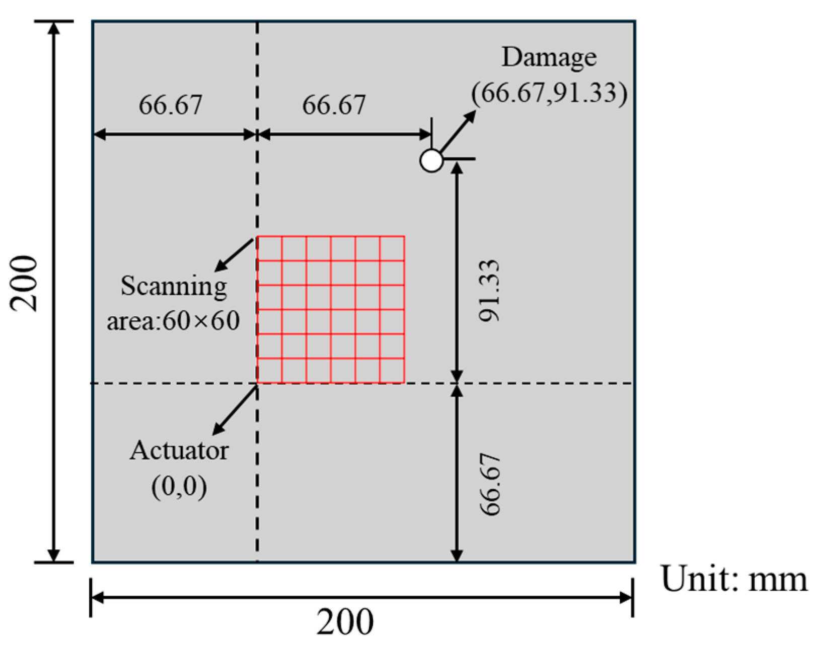
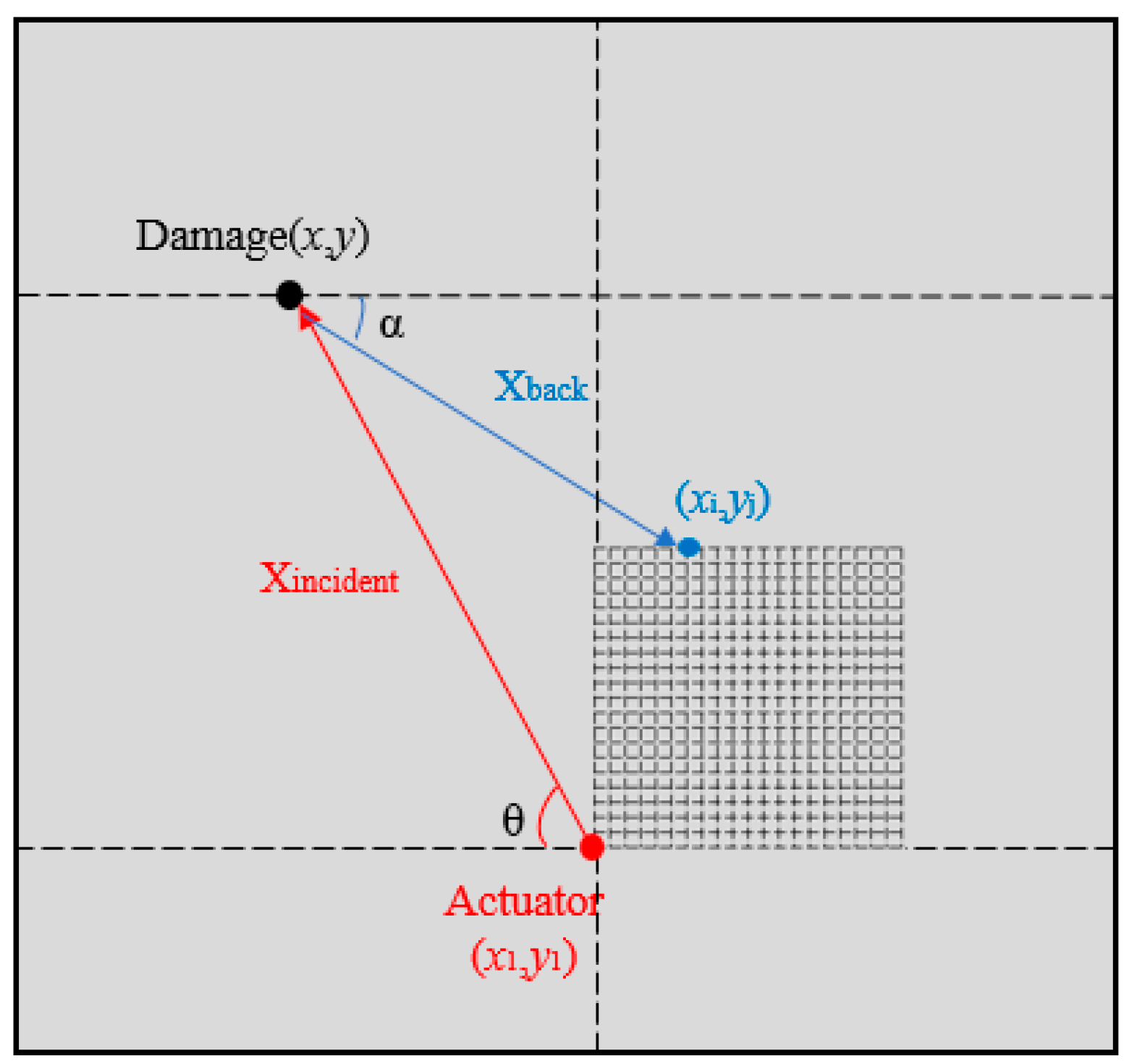
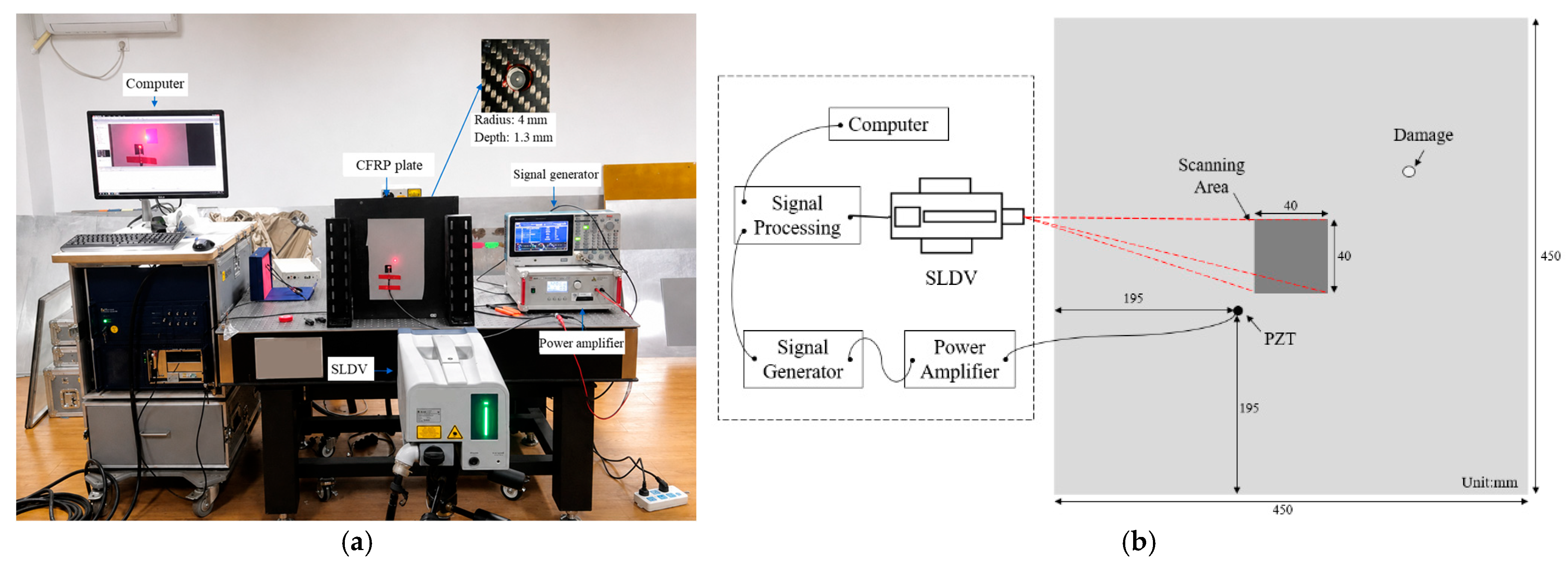
The finite-element model of the damaged aluminum plate established in this study is shown in Figure 2. The red line in the figure denotes the scanning path used to extract spatiotemporal information. The scanning length is 60 mm, the interval between adjacent scanning points is 0.5 mm, and the scanning direction is 45°. The dimensions of the aluminum-plate model are 200 mm × 200 mm × 1 mm. The excitation point is located at one-third of the distance from both the lower boundary and the left boundary. The diameter of the excitation region is 6 mm, and the diameter of the through-hole damage is 8 mm, with its center located at (68.67 mm, 91.33 mm). The material parameters of the aluminum plate are as follows: elastic modulus, 70 GPa; Poisson’s ratio, 0.33; density, 2700 kg/m³.

In the numerical simulation, a linear chirp signal is used to excite ultrasonic guided waves. When guided waves propagate in the plate and encounter damage or boundaries, both damage-reflected waves and boundary-reflected waves are generated. For a numerical model of relatively small size, the energy of the boundary reflections may even exceed that of the damage reflections, thereby severely affecting the final imaging results. In experiments, however, the actual plate structure is larger, and the boundary reflections are therefore usually weaker than those in the numerical model. To reduce this discrepancy, low-reflection boundaries are adopted in the numerical model, and a Rayleigh damping layer with a width of 20 mm is arranged along the model edges. The Rayleigh mass-damping coefficient is taken as 2 × 10⁵, and the Rayleigh stiffness-damping coefficient is taken as 5 × 10⁻⁷. Meanwhile, in order to ensure simulation accuracy, the element size should satisfy

$$L\le {\displaystyle \frac{{\lambda }_{\min }}{10}}$$

(17)

where L denotes the finite-element mesh size and λ_min denotes the shortest wavelength of the Lamb wave.

In this study, considering the distinguishability of the A₀ and S₀ modes under broadband excitation as well as the requirements of imaging analysis, and given that the S₀ modal response is relatively weak in the lower frequency range and is therefore unfavorable for stable separation and comparative analysis of the two modes, a linear chirp signal with a bandwidth of 250–550 kHz was selected as the excitation; thus, the highest frequency was 550 kHz. Correspondingly, the wavelength of the S₀ mode is 9.6 mm, whereas that of the A₀ mode is 3.56 mm. By comprehensively considering computational cost and solution accuracy, a refined mesh is adopted in the damage region and the excitation region, while the mesh size in the remaining regions is 0.35 mm, and two swept elements are arranged through the thickness direction.

In addition to solution accuracy, transient dynamic analysis must also satisfy the requirements of numerical stability and convergence. According to the Newmark time-integration scheme, at least 20 time steps are required within one Lamb-wave period. Its expression is

$$\Delta t\le {\displaystyle \frac{1}{20f_{\max }}}$$

(18)

where ∆t denotes the time step and f_max denotes the highest frequency within the selected frequency band. By comprehensively considering overall computational efficiency, the time step is set to 0.05 μs.

3.2. Simulation Results of Modal Superposition Imaging Under Chirp Excitation

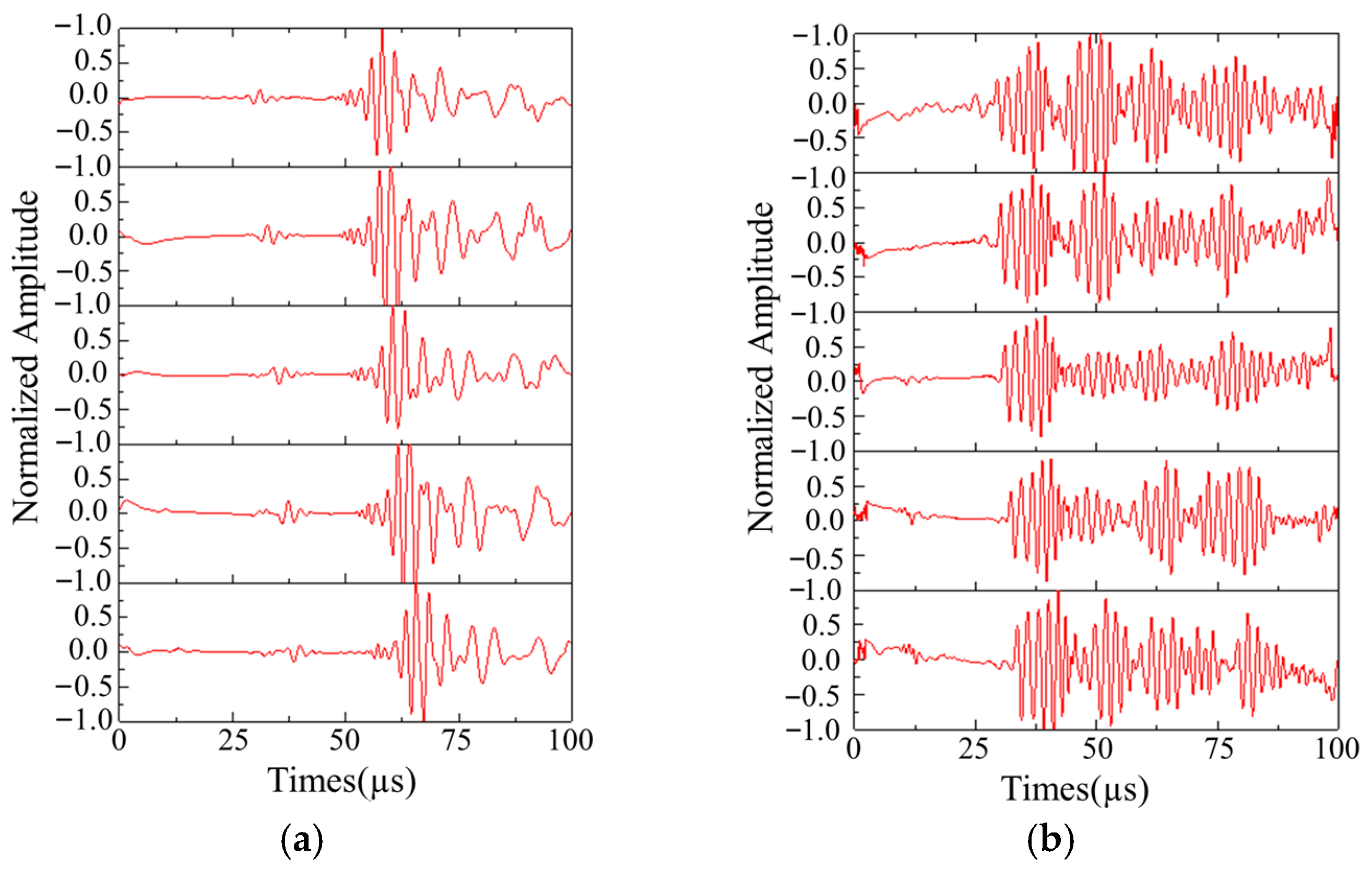
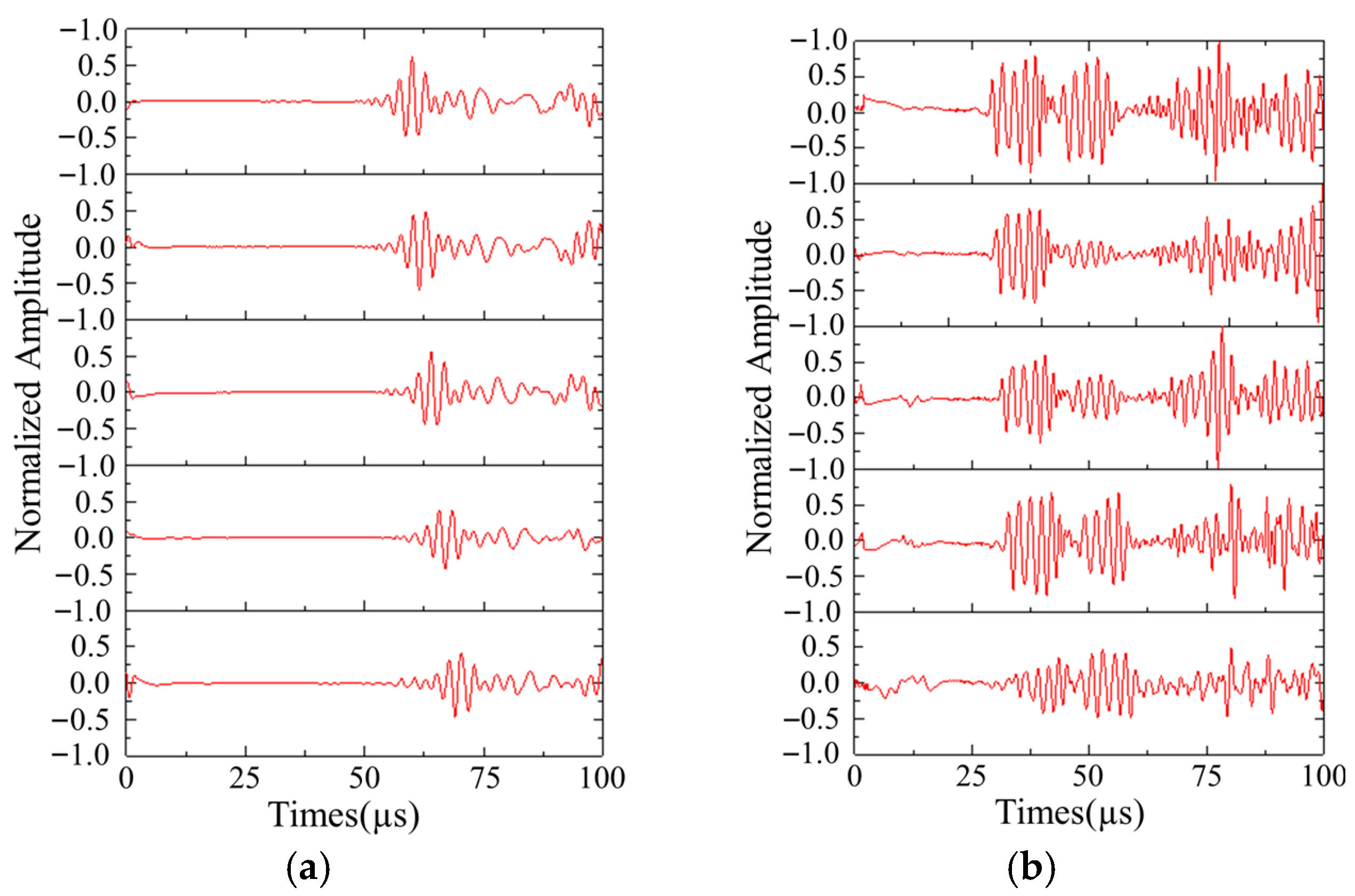
In damage imaging, a 12 × 12 array is selected. The position of the first array element is (5 mm, 5 mm), and that of the last array element is (60 mm, 60 mm), with an element spacing of 5 mm. Figure 3a shows the reflected responses acquired by different array elements after extraction of the A₀ mode, where the wave packet with the largest amplitude corresponds to the damage-reflected wave of the A₀ mode. Figure 3b shows the S₀ mode response, in which the earliest arriving wave packet is the S₀ mode damage-reflected wave, whereas the subsequent wave packets are mainly redundant information such as boundary reflections.

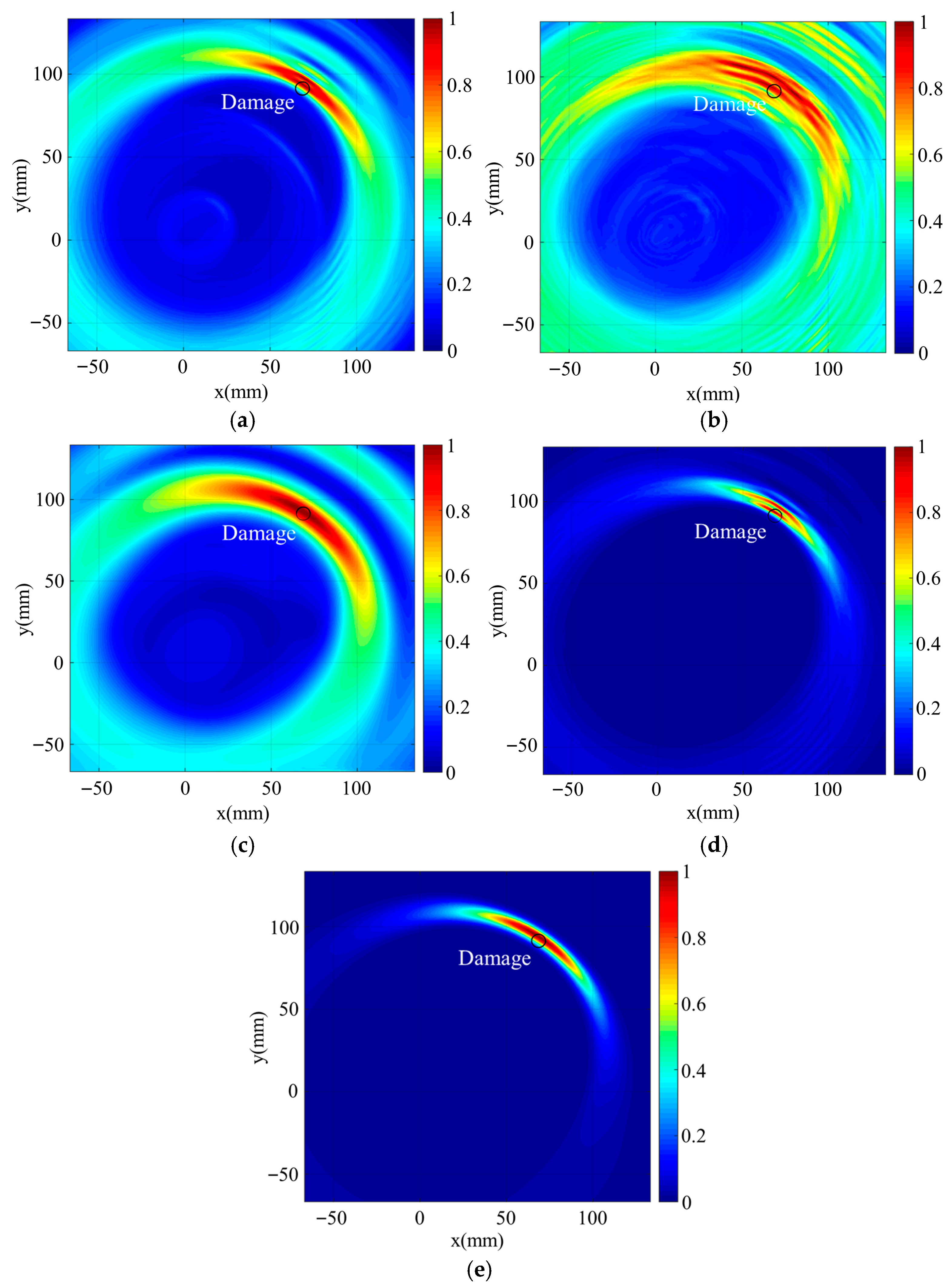
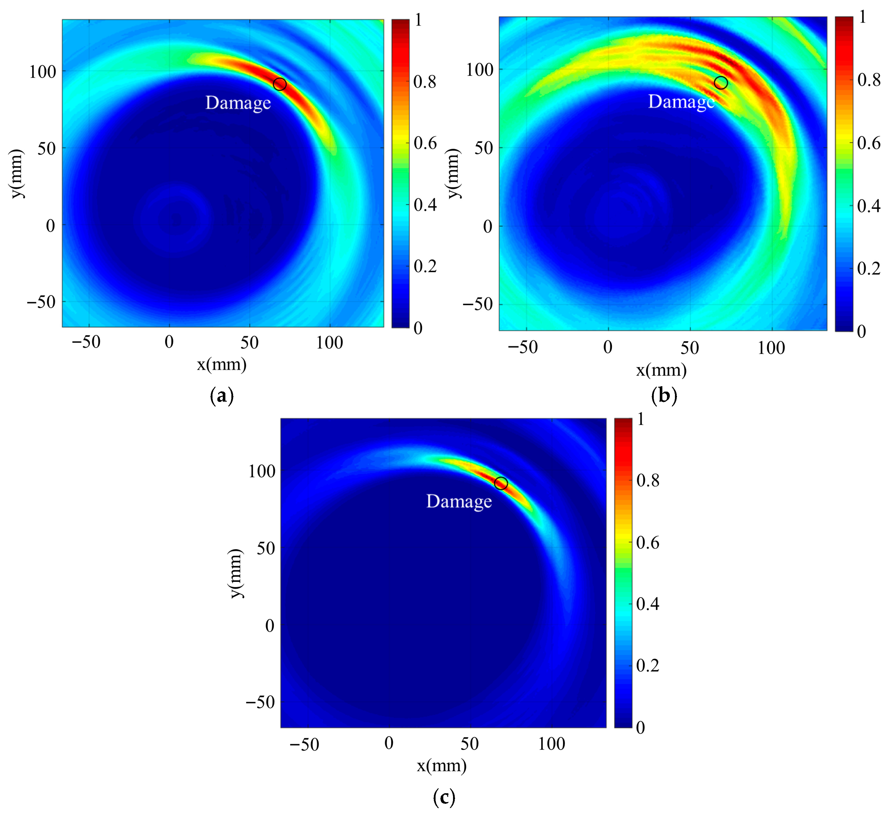
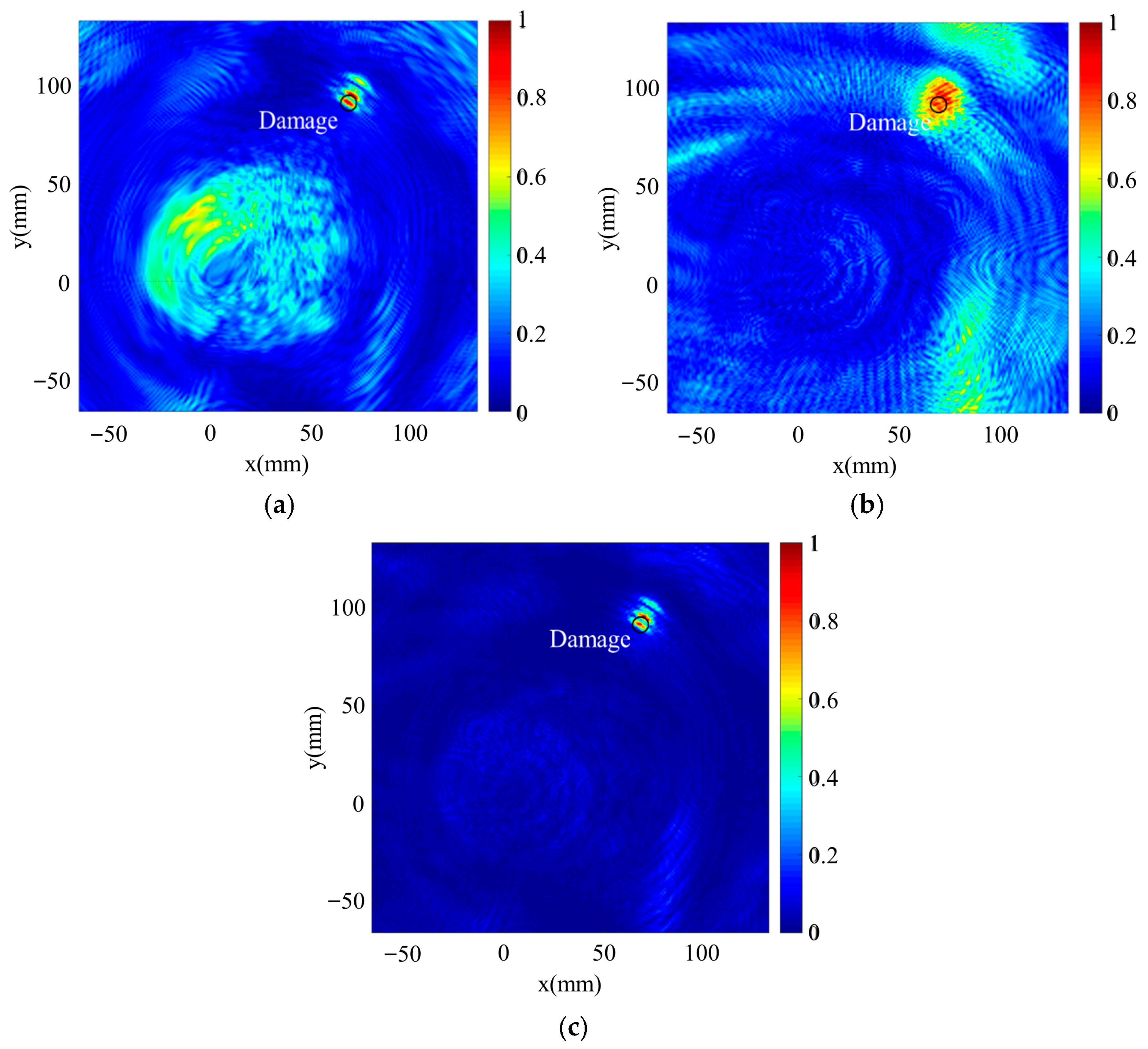
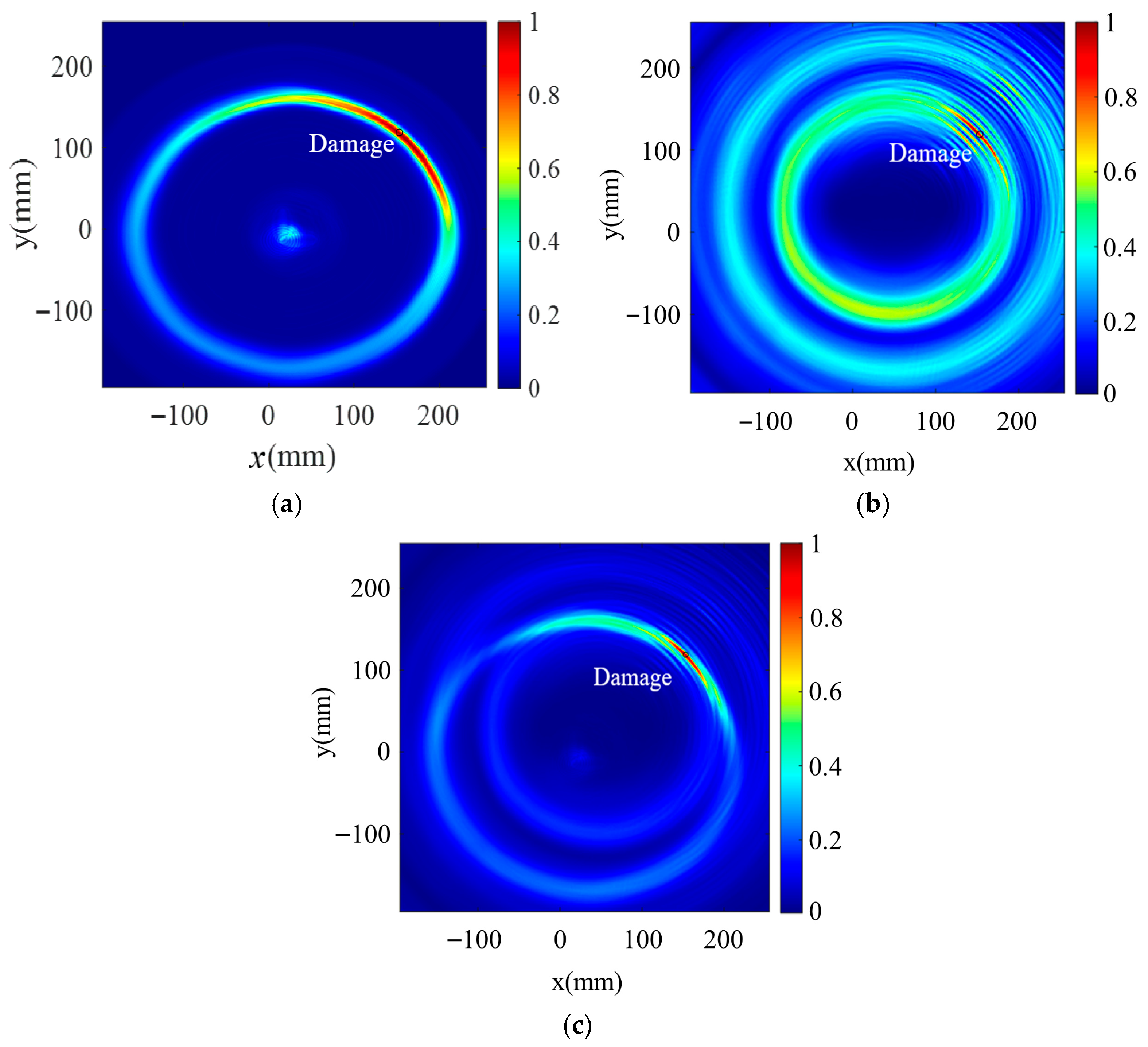
The selected array-element signals were imaged by the time-domain CSM algorithm through separated-modal superposition. The time-domain imaging results are shown in Figure 4, where Figure 4a,b present the time-domain CSM imaging results of the A₀ and S₀ modes, respectively; Figure 4c,d present the imaging results obtained by amplitude addition and amplitude multiplication of the S₀ and A₀ modes, respectively; and Figure 4e presents the imaging result obtained after additive–multiplicative modal fusion. The black circle in the figure denotes the true damage location. By comparing the two single-modal results, it can be seen that the damage-imaging region of the S₀ mode is wider than that of the A₀ mode, and the image purity is relatively lower. Neither of the two single-modal images is ideal when used alone. After image-data fusion, information from the two modes is combined. Compared with single-modal imaging, the damage-imaging region after modal superposition is significantly reduced, and the localization capability is improved. Through comparison, it can be seen that amplitude multiplication and additive–multiplicative modal fusion perform better than amplitude addition. Compared with the damage-imaging results obtained from a single mode, more accurate damage-imaging results can be achieved by using the image-data-fusion method to combine the sensitivities of different modes to damage. It can further be observed that the damage-imaging area can be reduced by means of data-fusion, and that both amplitude multiplication and additive–multiplicative modal fusion produce smaller damage-imaging regions and higher localization accuracy than amplitude addition.

In order to further quantitatively compare the localization performance of different imaging methods, the damage-imaging results were evaluated from three aspects, namely the coordinate error of the peak-amplitude point, RMSE, and UIQI, as shown in

Table 1. Error analysis of damage imaging results in the time domain.

Method	Coordinate Error of the Maximum Amplitude Point (mm)	RMSE	UIQI
A0 time-domain imaging	2.98	0.3936	0.0014
S0 time-domain imaging	3.07	0.5621	0.0009
Modal summation imaging	0.23	0.4398	0.0018
Modal multiplication imaging	0.23	0.2427	0.0087
Additive–multiplicative fusion imaging	0.23	0.2163	0.0103

. It can be seen from the table that the coordinate errors of the damage-imaging results for the single A₀ mode, single S₀ mode, modal addition, modal multiplication, and additive–multiplicative modal fusion are 2.98 mm, 3.07 mm, 0.23 mm, 0.23 mm, and 0.23 mm, respectively. The localization results for the single A₀ mode, single S₀ mode, modal addition, modal multiplication, and additive–multiplicative modal fusion are all located within the damage range (≤4 mm), but the localization errors are significantly reduced after multimodal fusion. The corresponding RMSE values are 0.3936, 0.5621, 0.4398, 0.2427, and 0.2163, respectively, and the UIQI values are 0.0014, 0.0009, 0.0018, 0.0087, and 0.0103, respectively. Although the coordinate errors of the damage-localization results for modal addition, modal multiplication, and additive–multiplicative modal fusion are identical, additive–multiplicative modal fusion yields the smallest RMSE and the largest UIQI. This indicates that, compared with the damage-imaging results of the single A₀ mode, single S₀ mode, modal addition, and modal multiplication, the additive–multiplicative modal fusion result shows the smallest discrepancy from the actual damage and better overall performance.

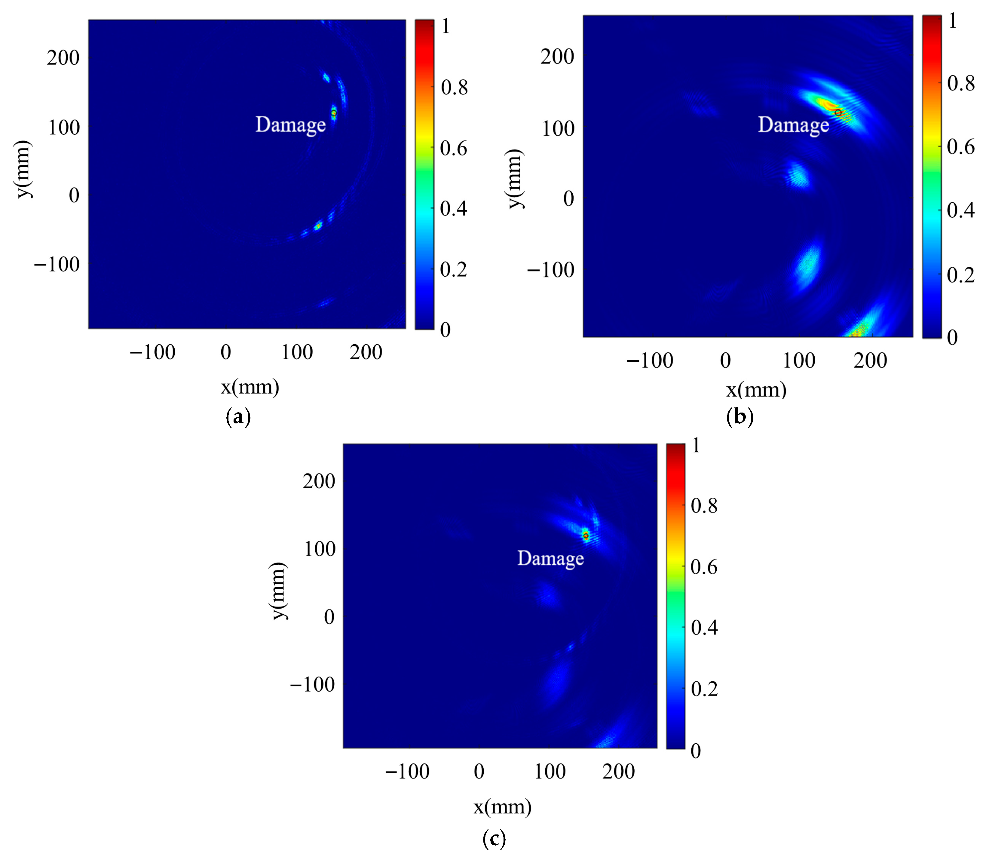
On the basis of time-domain CSM imaging, the selected array signals were further subjected to modal superposition imaging by using the f-k domain CSM algorithm, as shown in Figure 5. 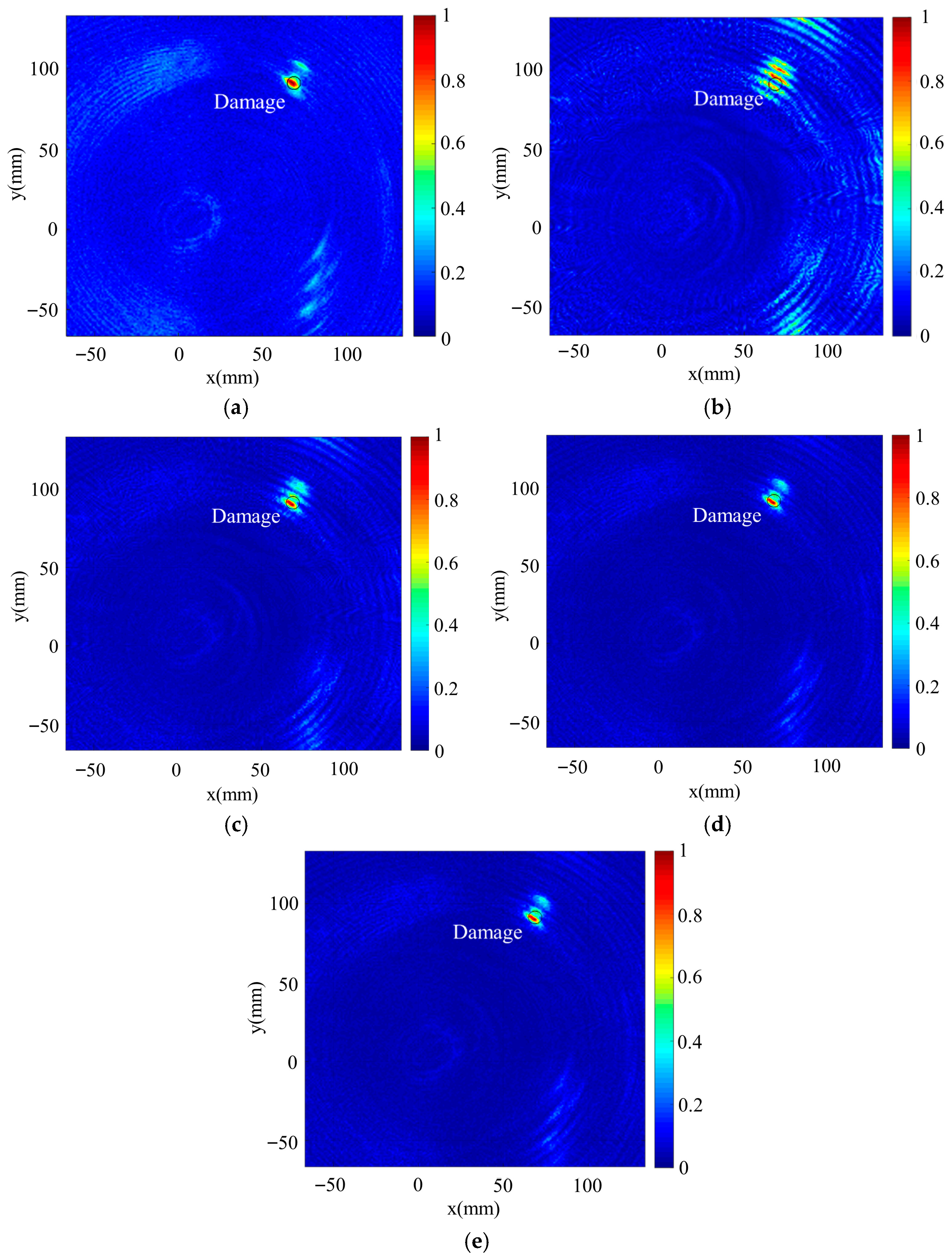Figure 5a,b show the f-k domain CSM imaging results of the A₀ and S₀ modes, respectively; Figure 5c,d show the imaging results obtained by amplitude addition and amplitude multiplication of the S₀ and A₀ modes, respectively; and Figure 5e shows the imaging result obtained after additive–multiplicative modal fusion. The brightest pixel represents the center of the simulated damage image, and the black circle represents the actual damage location. By comparing the two single-modal results, it can be seen that, consistent with the conclusion obtained for time-domain CSM, the damage-imaging region of the S₀ mode is wider than that of the A₀ mode, and the image purity is also relatively lower. Neither of the two single-modal images is ideal when used alone. After image-data fusion, the information from the two modes is combined. Compared with single-modal imaging, the damage-imaging region after modal superposition is significantly reduced, and the localization capability is improved. It can further be observed that, for f-k domain CSM imaging, the damage-imaging area can also be reduced by using the data-fusion method, and that both amplitude multiplication and additive–multiplicative modal fusion produce smaller damage-imaging regions and higher localization accuracy than amplitude addition.

As shown in

Table 2. Analysis of f-k domain error-evaluation indicators.

Method	Coordinate Error of the Maximum Amplitude Point (mm)	RMSE	UIQI
A0 imaging in the f-k domain	1.87	0.1473	0.0315
S0 imaging in the f-k domain	4.58	0.2156	0.0143
Modal summation imaging	0.81	0.1253	0.0434
Modal multiplication imaging	0.81	0.0926	0.0629
Additive–multiplicative fusion imaging	0.81	0.0718	0.0783

, the damage-imaging results of the five imaging methods in the f-k domain were evaluated from three aspects, namely the coordinate error of the peak-amplitude point, RMSE, and UIQI. It can be seen that the coordinate errors of the damage-imaging results for the single A₀ mode, single S₀ mode, modal addition, modal multiplication, and additive–multiplicative modal fusion are 1.87 mm, 4.58 mm, 0.81 mm, 0.81 mm, and 0.81 mm, respectively. The localization results for the A₀ mode, modal addition, modal multiplication, and additive–multiplicative modal fusion are all located within the damage range (≤4 mm), whereas the error of the single S₀ mode exceeds the damage range. The corresponding RMSE values are 0.1473, 0.2156, 0.1253, 0.0926, and 0.0718, respectively, and the corresponding UIQI values are 0.0315, 0.0143, 0.0434, 0.0629, and 0.0783, respectively. Although the coordinate errors of the damage-localization results for modal addition, modal multiplication, and additive–multiplicative modal fusion are identical, additive–multiplicative modal fusion yields the smallest coordinate error, the smallest RMSE, and the largest UIQI. This indicates that, compared with the damage-imaging results of the single A₀ mode, single S₀ mode, modal addition, and modal multiplication, the additive–multiplicative modal fusion result exhibits the smallest discrepancy from the actual damage and superior performance.

It should be noted that boundary reflections remain one of the major factors affecting the current simulation-imaging quality, especially for the S₀ mode. Although low-reflection boundaries and Rayleigh damping layers were adopted in the numerical model to reduce the interference of boundary reflections with damage imaging, the residual boundary-reflection components were not completely eliminated. Compared with the A₀ mode, the S₀ mode propagates at a higher velocity and therefore travels a longer path within the same sampling time window, making it more likely to overlap in space and time with residual boundary-reflection components. As a result, the imaging region is expanded, the background response is enhanced, and the localization error is increased. This is also one of the main reasons why the single-modal result of the S₀ mode is inferior to that of the A₀ mode in the simulations. Meanwhile, additive–multiplicative modal fusion can suppress inconsistent background spurious responses among different modes to a certain extent; therefore, the fused result still shows a more compact damage region and higher localization accuracy.

Overall, because the contributions of all frequency components within the selected frequency band and the dispersion effect are comprehensively taken into account, f-k domain CSM performs better than time-domain CSM in terms of single-modal imaging and image compactness. At the same time, the proposed additive–multiplicative modal-fusion method also shows certain advantages over conventional modal addition and modal multiplication in terms of imaging quality and damage-localization performance. Therefore, the feasibility of the proposed f-k domain CSM imaging algorithm under broadband chirp excitation is verified through numerical simulations.

4. Experimental Investigation of Damage Imaging Under Chirp Excitation

4.1. Experimental Setup

In order to verify the damage-imaging results under chirp excitation, an experimental platform was established for the aluminum plate, as shown in Figure 6. The excitation signal was generated by a signal generator, amplified by a power amplifier, and then applied to the plate through a piezoelectric transducer (PZT). The vibration response within the scanning region was measured by the SLDV laser head, and the acquired time-domain signals were then transmitted back to the signal-processing system. Meanwhile, the output of the signal generator was synchronized with the signal processor, so that synchronous observation of the excitation signal and the received signal could be achieved. The sampling frequency of the SLDV was 5 MHz. The dimensions of the aluminum plate used in the experiment were 500 mm × 500 mm, and a 200 mm × 200 mm region was selected as the imaging area. The PZT was placed at the coordinate origin (0 mm, 0 mm), and the PZT used in the experiment had a diameter of 10 mm and a thickness of 0.7 mm. The damage center was located at (68.67 mm, 91.33 mm), and the damage diameter was 8 mm. In order to ensure the simultaneous existence of multiple modes, a linear chirp signal of 250–550 kHz was used for damage excitation and detection.

4.2. Experimental Results and Discussion

A 12 × 12 array was used for the final damage imaging. The position of the first array element is (5 mm, 5 mm), and that of the last array element is (60 mm, 60 mm), with an element spacing of 5 mm. Figure 7 shows the filtered reflected responses of several array elements. In Figure 7a, the wave packet with the largest amplitude in the A₀ mode corresponds to the damage reflection, whereas the remaining wave packets mainly correspond to redundant information such as boundary reflections. In Figure 7b, the earliest arriving wave packet of the S₀ mode corresponds to the damage reflection, whereas the subsequent wave packets are likewise mainly composed of redundant information such as boundary reflections.

The CSM method was first used to perform time-domain imaging of the selected array signals. Figure 8a,b present the single-modal imaging results, where the black circle denotes the true damage location. In Figure 8a, the A₀ mode image is more concentrated than the S₀ mode image, but its high-response region is still larger than the actual defect size. For the S₀ mode, the high-response region is more dispersed and the imaging quality is poorer. Therefore, among the single-modal time-domain results, the A₀ mode performs better than the S₀ mode, although the imaging quality of both remains limited. Figure 8c shows the image obtained after data fusion through additive–multiplicative modal combination. The damage-imaging result becomes more compact, indicating that modal superposition can, to a certain extent, enhance damage characterization and improve imaging quality.

As shown in

Table 3. Analysis of time-domain error-evaluation indicators.

Method	Coordinate Error of the Maximum Amplitude Point (mm)	RMSE	UIQI
A0 time-domain imaging	7.21	0.3824	0.0012
S0 time-domain imaging	7.44	0.4973	0.0007
Additive–multiplicative fusion imaging	5.94	0.2127	0.0276

, the damage-localization and imaging results of the proposed additive–multiplicative modal-fusion method, the single A₀-mode method, and the single S₀-mode method in the time domain were evaluated in terms of the coordinate error of the peak-amplitude point, RMSE, and UIQI. It can be seen from the table that the coordinate errors of the damage-imaging results for the single A₀ mode, single S₀ mode, and additive–multiplicative modal fusion are 7.21 mm, 7.44 mm, and 5.94 mm, respectively. Although the localization performance is improved after data fusion by additive–multiplicative modal fusion compared with that of single-modal imaging, the result still lies outside the damage range. The corresponding RMSE values are 0.3824, 0.4973, and 0.2127, respectively, and the corresponding UIQI values are 0.0012, 0.0007, and 0.0276, respectively. It can be seen from the table that the additive–multiplicative modal fusion result yields the smallest coordinate error, the smallest RMSE, and the largest UIQI. This indicates that, compared with the damage-localization imaging results of the single A₀ mode and the single S₀ mode, the additive–multiplicative modal fusion result shows the smallest discrepancy from the actual damage and better performance.

Therefore, under experimental conditions, time-domain CSM can achieve preliminary damage localization, but problems such as strong background response and limited localization accuracy still remain. To further improve damage-identification capability under broadband excitation, the f-k domain imaging method is required. The f-k domain CSM imaging results are shown in Figure 9. The black circle denotes the actual damage location, and the brightest pixel denotes the center of the experimental image. Figure 9a presents the single A₀ mode result, and Figure 9b presents the single S₀ mode result. The A₀ mode image is more concentrated than its time-domain counterpart, indicating that the localization accuracy is significantly improved, although a relatively large green patch still exists in the middle of the image and the image quality remains limited. Compared with time-domain imaging, the S₀ mode result likewise shows a more concentrated damage region and better localization performance. Figure 9c shows the imaging result obtained after additive–multiplicative modal fusion. The damage region is further compressed, the background spurious response is significantly weakened, and the overall image quality and localization stability are both improved.

As shown in

Table 4. Analysis of f-k domain error-evaluation indicators.

Method	Coordinate Error of the Maximum Amplitude Point (mm)	RMSE	UIQI
A0 imaging in the f-k domain	2.13	0.3383	0.0068
S0 imaging in the f-k domain	2.74	0.4211	0.0037
Additive–multiplicative fusion imaging	0.91	0.1284	0.0786

, the damage-localization and imaging results of the proposed additive–multiplicative modal-fusion method and the single A₀-mode and single S₀-mode methods in the f-k domain were evaluated in terms of the coordinate error of the peak-amplitude point, RMSE, and UIQI. It can be seen from the table that the damage-imaging results of the single A₀ mode and the single S₀ mode are both located within the damage range (≤4 mm), with errors of 2.13 mm and 2.74 mm, respectively. Compared with the corresponding single-modal damage-imaging results in the time domain, the localization accuracy is improved. After additive–multiplicative modal fusion, the localization error is further reduced to 0.91 mm. Meanwhile, the corresponding RMSE values are 0.3383, 0.4211, and 0.1284, and the corresponding UIQI values are 0.0068, 0.0037, and 0.0786. It can be seen from the table that the additive–multiplicative modal fusion result yields the smallest coordinate error, the smallest RMSE, and the largest UIQI. This indicates that, compared with the damage-localization imaging results of the single A₀ mode and the single S₀ mode, the additive–multiplicative modal fusion result shows the smallest discrepancy from the actual damage and better performance.

In order to demonstrate the engineering feasibility of the algorithm, the processing times required by the time-domain CSM and the f-k domain CSM were compared. A unified computing platform was used, consisting of an Intel(R) Core(TM) i5-13400 processor, 32 GB memory, and Matlab R2024a. Under the current dataset and implementation process, the total processing time of the time-domain CSM route was approximately 3.2 s, whereas the processing time of the f-k domain CSM route for a single mode was approximately 8.7 s. For additive–multiplicative modal fusion, the total processing time of the f-k domain route was 13.9 s. The higher computational time of the f-k domain method is mainly attributed to the need for modal separation in the f-k domain and coherent accumulation of multiple retained frequency components during imaging. Nevertheless, the required imaging time remains acceptable, and the proposed method improves both image compactness and localization accuracy.

Because the dimensions of the plate structure are finite, the acquired guided-wave signals contain not only damage reflections but also redundant components such as boundary reflections, and these components affect the purity and localization stability of single-modal imaging to a certain extent. For the S₀ mode, this effect is more pronounced and is manifested as a more expanded damage region and a stronger background spurious response. Although f-k domain modal separation can weaken part of the interference by retaining effective frequency-wavenumber components near the target mode, its influence cannot be completely eliminated when boundary reflections overlap with damage reflections within the same modal branch. Therefore, boundary reflections remain an inherent limitation that must be addressed by the current method under experimental conditions. Overall, the experimental results are basically consistent with the simulation results, indicating that the imaging method based on f-k domain modal separation and additive–multiplicative modal fusion possesses good damage-detection capability under broadband chirp excitation.

4.3. Experimental Validation on a CFRP Plate

In order to verify the applicability of the proposed algorithm, a damage-detection experimental system for a composite plate was established, as shown in Figure 10a. Figure 10b presents the composite-plate damage-detection experimental system together with its specific positional arrangement and instrument connections. The PZT was positioned slightly below and to the left of the center of the plate, at a distance of 195 mm from the nearest boundary. The position of the PZT was set as the origin (0 mm, 0 mm). The coordinates of the prefabricated flat-bottom-hole damage were (153 mm, 119 mm), and the blind-hole damage had a radius of 4 mm and a depth of 1.3 mm. The SLDV scanning area was located in the 40 mm × 40 mm region at the center of the plate.

The specific material parameters of the orthotropic CFRP composite plate used in the experiment are listed in

Table 5. Physical property parameters of the CFRP composite plate.

Density (kg/m3)	Thickness (mm)	E1 (GPa)	E2 (GPa)	E3 (GPa)	G12 (GPa)	G13 (GPa)	G23 (GPa)	v12	v13	v23
1520	2	135	10	10	5.5	4.5	5.5	0.0183	0.25	0.45

. The dimensions of the selected plate were 450 mm × 450 mm × 2 mm. The driving signal was generated by a function generator, amplified by a power amplifier, and output through the PZT. The displacement signals within the designed scanning area on the CFRP plate were acquired by the SLDV.

The received array-element signals were first processed for damage imaging by using the CSM method. Figure 11a,b present the time-domain single-modal imaging results of the A₀ and S₀ modes, respectively, in which the black circle denotes the true damage location. By comparing the two results, it can be seen that, relative to the actual damage, the damage-detection results of both modes are obviously larger and exceed the actual damage range. In addition, because the amplitude difference between the damage signal and the boundary-reflection signal of the S₀ mode is less pronounced than that of the A₀ mode, many regions with high pixel values are present in the S₀ result, thereby increasing the difficulty of interpretation. By applying the proposed additive–multiplicative modal-fusion imaging method to the two modal results, the fused damage-imaging result shown in Figure 11c is obtained. It can be seen that the damage-imaging result becomes more compact after additive–multiplicative modal fusion, thereby verifying the feasibility of the additive–multiplicative modal-fusion method for orthotropic CFRP composite plates.

Table 6. Analysis of time-domain error-evaluation indicators.

Method	Coordinate Error of the Maximum Amplitude Point (mm)	RMSE	UIQI
A0 time-domain imaging	3.7	0.4763	0.0032
S0 time-domain imaging	5.94	0.5676	0.0022
Additive–multiplicative fusion imaging	2.34	0.1661	0.0102

presents the analysis of time-domain error-evaluation indicators, in which the damage results were evaluated from three aspects, namely the coordinate error of the peak-amplitude point, RMSE, and UIQI. It can be seen from the table that the coordinate errors of the damage-imaging results for the single A₀ mode, the single S₀ mode, and the additive–multiplicative modal fusion are 3.7 mm, 5.94 mm, and 2.34 mm, respectively. The localization results of the A₀ mode and the fused result are both located within the damage range (≤4 mm), whereas the error of the single S₀ mode exceeds the damage range. The corresponding RMSE values are 0.4763, 0.5676, and 0.1661, respectively, and the corresponding UIQI values are 0.0032, 0.0022, and 0.0102, respectively. It can be seen from the table that the additive–multiplicative modal fusion result yields the smallest coordinate error, the smallest RMSE, and the largest UIQI. This indicates that, compared with the results of the single A₀ and S₀ modes, the additive–multiplicative modal fusion result shows the smallest discrepancy from the actual damage and better performance. It can also be seen from Figure 11 that the high-response area of the damage is smaller in the fused result.

Compared with time-domain imaging, f-k domain imaging can take all frequency components containing damage information within the selected band into account, thereby acquiring more damage information to improve the imaging accuracy. The received array-element signals were then processed for damage imaging. Figure 12a,b show the f-k domain single-modal damage-imaging results of the A₀ and S₀ modes, respectively, and the actual damage location is marked by a black circle in the figures. From the analysis of the two single-modal images, it can be seen that the damage-region areas of both modal images are relatively concentrated, but isolated regions with high pixel values still exist in both images. These spurious images affect the judgment of damage localization, and the overall image purity is poor. By applying the proposed additive–multiplicative modal-fusion imaging method to the two modal results, the fused damage-imaging result shown in Figure 12c is obtained. It can be seen that the damage-imaging result becomes more compact after additive–multiplicative modal fusion, indicating that modal superposition can enhance damage characterization and improve imaging quality to a certain extent.

Table 7. Analysis of f-k domain error-evaluation indicators.

Method	Coordinate Error of the Maximum Amplitude Point (mm)	RMSE	UIQI
A0 imaging in the f-k domain	3.28	0.2464	0.0429
S0 imaging in the f-k domain	4	0.2829	0.0113
Additive–multiplicative fusion imaging	2.06	0.1139	0.0858

presents the analysis of the f-k domain error-evaluation indicators for the experiment, in which the damage results were evaluated from three aspects, namely the coordinate error of the peak-amplitude point, RMSE, and UIQI. It can be seen from the table that the coordinate errors of the damage-imaging results for the single A₀ mode, the single S₀ mode, and the fused result are 3.28 mm, 4 mm, and 2.06 mm, respectively, all of which lie within the damage range (≤4 mm). The corresponding RMSE values are 0.2464, 0.2829, and 0.1139, respectively, and the corresponding UIQI values are 0.0429, 0.0113, and 0.0858, respectively. It can be seen from the table that the fused result yields the smallest coordinate error, the smallest RMSE, and the largest UIQI. Compared with the results of the single A₀ and S₀ modes, the fused result shows the smallest discrepancy from the actual damage and better performance.

5. Conclusions

In this study, a broadband guided-wave damage imaging method based on f-k domain mode separation and additive–multiplicative modal fusion was proposed through numerical simulations and experimental investigations, and the validation objects were extended from an isotropic aluminum plate containing through-hole defects to an orthotropic composite plate containing blind-hole defects. The results indicate that the f-k domain mode separation can provide effective input for A₀- and S₀-mode imaging, while the additive–multiplicative modal fusion can further improve the compactness and localization accuracy of the damage region. Compared with time-domain CSM imaging, although a longer computation time is required by f-k domain CSM, the effective frequency components within the selected frequency band can be more fully utilized and the guided-wave dispersion effect can be taken into account, thereby yielding more stable and more compact imaging results. Both the simulation and experimental results demonstrate that the proposed method exhibits good damage identification capability and promising application potential under broadband chirp excitation. It should be noted that the feasibility of the proposed method has, at present, still been mainly validated under the existing numerical and experimental conditions. Further investigations are still required in future work on plates with different sizes and geometrical shapes, on more complex damage forms such as cracks and delamination, and on issues including low signal-to-noise ratio conditions, repeatability, and the influence of boundary reflections, so that the engineering applicability of the proposed method can be evaluated more comprehensively.