Phase-Field Modeling of Fracture Propagation Patterns Under Proppant Support in Sequential Hydraulic Fracturing

Abstract

Numerical simulation of sequential fracturing in horizontal wells for shale gas and oil extraction requires careful consideration of mechanical interactions between proppant and fracture surfaces—a challenge that remains largely unresolved. This study proposes a novel phase-field model featuring a strain-based formulation and a width-dependent proppant reaction force. Unlike previous studies, we integrate an empirical propped force solution, adapted from established work to account for rock properties and proppant support, to capture nonlinear fracture closure. Results show that reaction stress models significantly dictate propped geometry. The model’s fracture length, width, and closure predictions are validated against theoretical solutions. We conducted a sensitivity analysis to evaluate how fracture deflection angles and widths vary with dimensionless fracture spacing, in situ stress contrast, and proppant strength. Numerical results show that proppants induce pronounced morphological asymmetry and distinct geometric discrepancies. Specifically, the heterogeneous support provided by proppants and the resulting stress redistribution alter fracture propagation paths, leading to an 8% reduction in fracture length and a marked difference in fracture orientation of approximately 80° between supported and unsupported fractures, highlighting the important role of proppants in governing fracture geometry. Both dimensionless fracture spacing and in situ stress contrast strongly influence fracture deflection, with proppant strength also contributing. The propped-force formulation is further extended to nonplanar fractures, enabling application to sequential fracturing with multiple fractures. These results highlight fracture propagation mechanisms and demonstrate the robustness of the proposed phase-field model.

1. Introduction

Hydraulic fracturing is a key technology for developing unconventional reservoirs such as shale gas, tight oil, and coalbed methane, enabling efficient hydrocarbon recovery from formations with extremely low permeability and porosity [1,2]. By injecting high-pressure fluid, it creates fractures that enhance reservoir connectivity and fluid flow [3]. Over the past few decades, this technique has transformed energy production, particularly in North America, and driven advances in modeling, treatment design, and reservoir characterization [4].

The first experimental application of hydraulic fracturing to enhance oil recovery was carried out in 1947 at the Gutan Field in Texas, USA. Although vertical wells dominated early hydraulic fracturing operations, horizontal well fracturing technologies, introduced in the 1980s, have demonstrated significantly higher production efficiency compared to vertical wells [5]. In recent years, staged fracturing has become a common practice in the development of unconventional reservoirs. By dividing a single well into multiple fracturing stages, this technique increases the stimulated reservoir volume and enhances production [6]. While hydraulic fracturing has revolutionized unconventional resource extraction, significant room for improvement remains. Statistical data from mature North American oil and gas fields reveal a critical challenge: approximately one-third of perforations fail to generate effective hydraulic fractures [7]. This highlights a substantial opportunity to enhance current techniques despite their successes [8]. 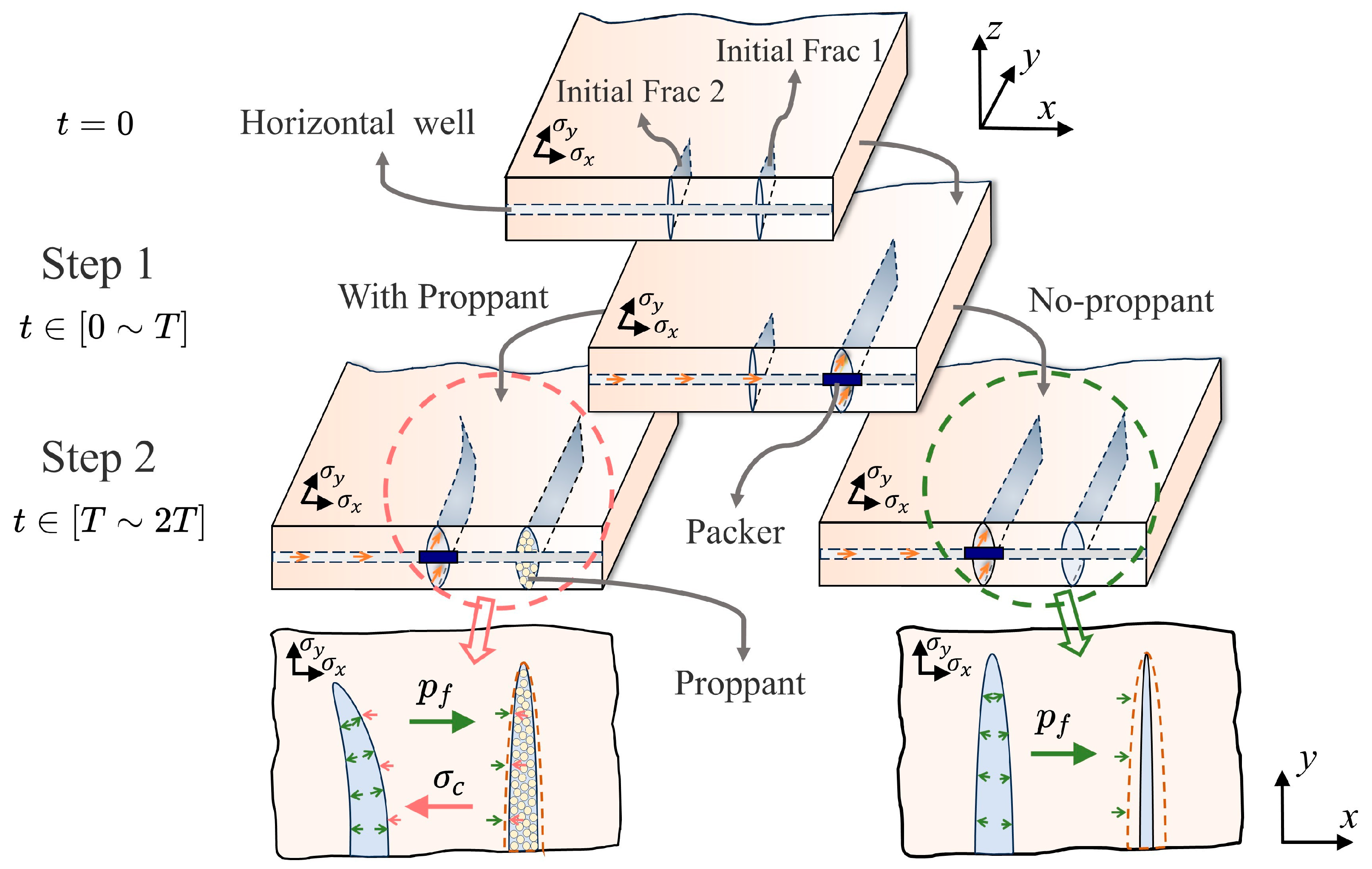Figure 1 illustrates a two-step sequential fracturing process. Initially, a fracture is created, and proppant is injected along with the fracturing fluid. This proppant is crucial for keeping the fracture open by preventing the fracture surfaces from closing after the fluid leaks off into the surrounding rock. Subsequently, a second fracture is initiated at a specific distance from the first. However, a key challenge arises with the propagation of these subsequent fractures: they often deflect. This deflection is primarily due to stress shadowing effects, where the in situ stress field is altered by the previously propped fractures. Such stress alterations can impede fracture propagation or even lead to unwanted fracture coalescence [9,10]. Addressing these stress shadowing effects is vital for optimizing multi-stage fracturing operations and maximizing resource recovery. Beyond conventional operations, the sensitivity of rock fracture behavior to diverse loading conditions and stress perturbations has been widely recognized. For example, cyclic in situ methane detonation fracturing can generate complex fracture networks through transient high-pressure loading [11], while thermal–cryogenic treatments consisting of cyclic heating and liquid nitrogen cooling induce fracture evolution and mechanical degradation in rock [12]. These studies indicate that fracture behavior is highly sensitive to loading conditions and stress perturbations, highlighting the critical role of stress evolution in controlling fracture propagation.

Many numerical models have been proposed to simulate hydraulic fracturing, such as Extended Finite Element Method (XFEM), Finite-discrete element method (FDEM), Discrete Fracture Network (DFN), Cohesive Zone Method (CZM), and Displacement Discontinuity Method (DDM) and Peridynamics (PD). XFEM enables crack propagation modeling without the need for remeshing, but struggles with convergence difficulties and three-dimensional (3D) problems with complex fracture geometries [13]. FDEM enables accurate simulation of both continuum deformation and fracture-induced discontinuities, effectively capturing crack initiation and dynamic propagation [14]. However, it typically requires fine meshing and is computationally intensive, particularly for large-scale three-dimensional problems [15,16]. DFN models efficiently simulate flow in pre-existing fracture networks, especially in large-scale settings, but they cannot capture the propagation of new fractures and offer limited interaction with the surrounding matrix, restricting its use in dynamic fracturing scenarios. CZM is widely used due to its physical clarity and ability to represent fracture toughness explicitly; however, it requires prior knowledge of crack paths or the placement of cohesive elements, making it less suitable for problems involving spontaneous and complex fracture evolution [17,18]. DDM is efficient for linear elastic materials with simple geometries but lacks accuracy in nonlinear or heterogeneous media [19,20]. PD naturally simulates fracture initiation, propagation, and branching without requiring additional criteria or remeshing, making it well-suited for modeling discontinuous media [21]. The Phase-Field Method (PFM) uses a continuous field to represent fractures, enabling the natural simulation of crack initiation, propagation, branching, and interaction without explicitly [22,23]. Its robustness and adaptability make PFM particularly well-suited for modeling hydraulic fracturing [24,25,26]. Beyond traditional fracture modeling, recent advances have extended variational phase-field approaches to account for frictional contact and non-penetration constraints, effectively preventing unphysical interpenetration [27]. In parallel, advanced fluid-driven phase-field formulations have emerged, utilizing hybrid-dimensional iterative schemes [28] and updated Lagrangian frameworks with geometric nonlinearity [29]. These developments, often complemented by dynamic mesh refinement, enable the robust simulation of coupled hyperelastic deformations and nonlinear fluid flow within a unified, versatile framework for complex multi-physics fracture processes.

Over the past decades, significant efforts have been dedicated to developing numerical models for simulating staged fracturing processes. These models have greatly advanced our understanding of fracture propagation behavior under multi-stage stimulation. Regarding the simulation of proppant distribution within fractures, current techniques primarily encompass multiphase flow models [30] and the Computational Fluid Dynamics–Discrete Element Method (CFD-DEM) [31]. In multiphase flow models, the injected mixture is simplified, with proppant particles treated as the solid phase and the fracturing fluid as the liquid phase. Conversely, CFD-DEM explicitly represents proppant as discrete 2D discs or 3D spheres, which are assumed to be rigid bodies interacting through collisions [32]. Additionally, the proppant transport model based on the phase-field method can accurately predict the concentration distribution of proppants [33]. Although these methods can capture the overall distribution of proppants within fractures, a critical gap remains: the accurate estimation of the complex interactions between the proppant and the fracture surfaces. Sesetty and Ghassemi [8] proposed a staged fracturing model using the DDM, which incorporated proppant support into the simulation framework. While the DDM offers valuable insights into stress interactions between fractures, its applicability in practical engineering scenarios is significantly constrained by fundamental limitations in handling nonlinear problems, such as elastoplastic deformation of rock, as well as the intricate processes of proppant crushing and compaction. These limitations ultimately compromise the accuracy and reliability of DDM in predicting real-world fracture propagation and reservoir performance. Tian et al. [34] introduced a staged fracturing model based on the XFEM, enabling the simulation of fracture initiation and propagation without explicit mesh alignment. However, this model neglected the mechanical contribution of proppants, leading to an underestimation of the stress shadowing effect—an important mechanism that influences the trajectory of subsequent fractures. Shi et al. [35] developed an XFEM-based framework incorporating the closure of propped fracture, in which proppants are assumed to be arranged in an idealized multilayer hexagonal close-packed structure, while neglecting proppant embedment into fracture surfaces. Liu et al. [36] proposed an XFEM model incorporating a spring-based representation of proppants. However, the spring elements, modeled as linear elastic units, cannot accurately capture the nonlinear mechanical behavior of proppants. More recently, Zhu et al. [37] proposed a PFM for simulating staged hydraulic fracturing processes. Although the model can simulate complex fracture geometries without requiring explicit fracture tracking algorithms, it does not account for proppant-induced reaction forces [38]. In summary, existing models are limited in their ability to represent the influence of proppant on fracture evolution within a unified framework that accounts for its dependence on fracture width behavior.

To address this limitation, this work presents a phase-field framework that incorporates a strain-based fracture width formulation coupled with a width-dependent proppant support representation. Unlike conventional linear models, our approach integrates the nonlinear coupling between proppant-induced reaction stress and fracture width evolution, thereby capturing the essential mechanical response of the proppant pack under closure stress. This combination enables the precise capturing of interaction forces between proppants and complex fracture walls. Although complex transport processes are simplified to a uniform distribution in this idealized scenario, the model remains a valuable tool for characterizing intricate fracture morphologies. Although complex transport processes are simplified to a uniform distribution in this idealized scenario, the model still provides useful insights into fracture morphologies, albeit with some limitations. By systematically analyzing parameter sensitivities, this research elucidates the mechanisms governing sequential fracture propagation, providing a theoretical foundation for more efficient reservoir stimulation.

2. Methodology

The phase-field model uses a smeared method for simulating crack propagation. This section introduces the phase-field equations governing fracture propagation, the model’s assumptions and the integration of a strain-based fracture width formulation coupled with the proppant-induced reaction stress.

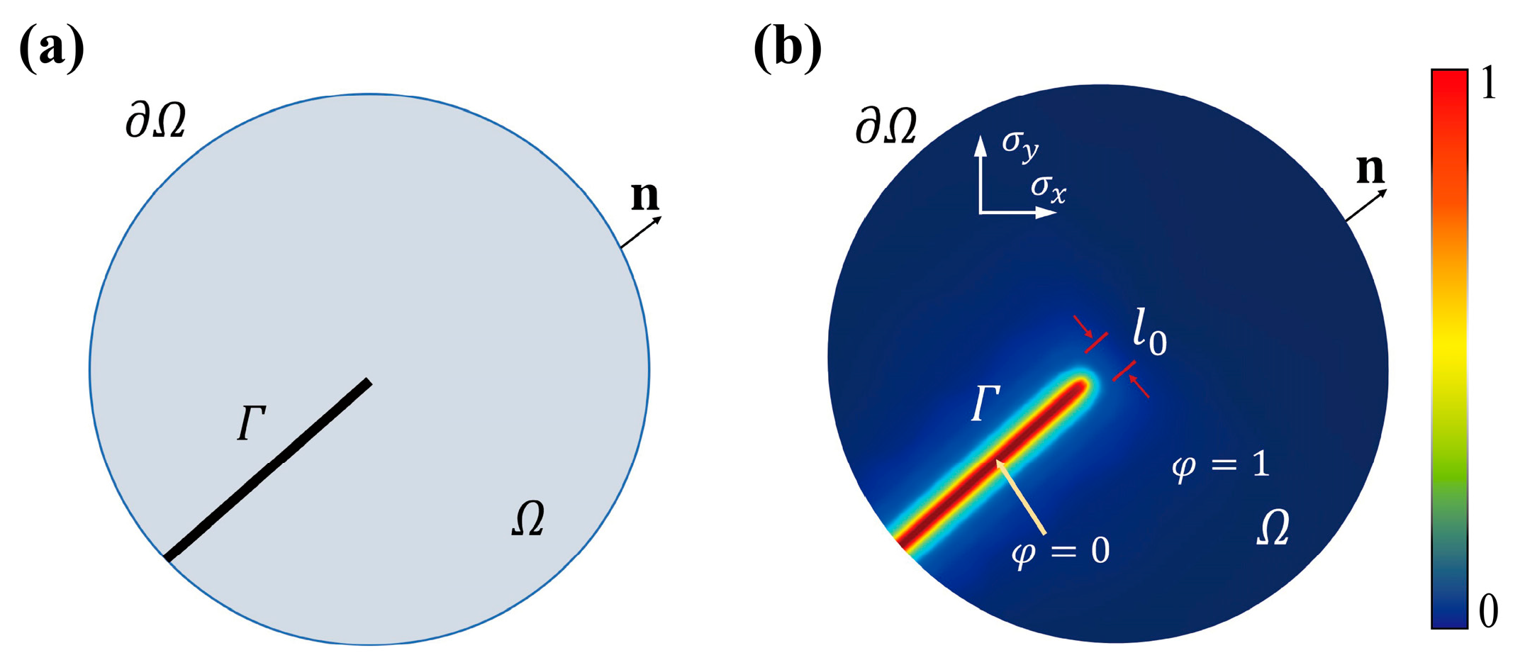
The phase-field method for fracture modeling is based on two fundamental physical fields: the vector-valued elastic field and the scalar-valued phase field. Typically, the phase-field model assumes an arbitrary bounded domain $\Omega$, which is composed of external boundary $\partial \Omega$ and internal boundary $\Gamma$. The diffusion crack topology (see Figure 2b) can be constructed based on the sharp crack topology (see Figure 2a) proposed by Miehe et al. [39], and described by using the field variable $\phi$. The phase-field is described by a scalar field $\phi (\mathrm{x},\mathrm{t})\in [0, 1]$, where $\phi =0$ represents the intact solid domain, $\phi =1$ denotes the fully damaged domain, and the intermediate region where $\phi$ lies between 0 and 1 is referred to as the transition domain, indicating partially damaged material. A length scale parameter $l_0$ is introduced to control the width of this transition domain [40]. In the initial state of the model, the intact solid region and the predefined initial crack are assigned values of $\phi =0$ and $\phi =1$, respectively.

2.1. Governing Equations of Phase-Field Method

According to the variational principle of fracture, the system’s behavior is governed by the competition between energy storage and dissipation. The total energy functional of the coupled system can be established as:

$$\Psi ={\Psi }^{\mathsf{\epsilon }}+{\Psi }^d-{\Psi }^k-{\Psi }^p+{\Psi }^c-{\Psi }^e$$

(1)

where ${\Psi }^{\epsilon }$ and ${\Psi }^d$ represent the elastic strain energy and the fracture dissipation energy, respectively. The term ${\Psi }^c$ accounts for the potential energy associated with proppant resistance, treated as a positive contribution because the mechanical reinforcement provided by the proppant effectively enhances the system’s internal energy storage. Conversely, the kinetic energy ${\Psi }^k$, the work done by fluid pressure ${\Psi }^p$, and the work done by external loads ${\Psi }^e$ are subtracted from the functional. Subtracting these external and inertial energy contributions ensures the functional correctly dictates the system’s equilibrium and evolution.

Kristensen et al. [41] proposed a formula for calculating the elastic energy of isotropic, homogeneous, linear elastic materials:

$${\Psi }^{\mathsf{\epsilon }}=\underset{\Omega }{\int }{\psi }_{\mathsf{\epsilon }}\left(\mathsf{\epsilon }\right)d\Omega$$

(2)

where the strain tensor $\mathsf{\epsilon }$ can be expressed in terms of the displacement field $\mathbf{u}$ as:

$$\mathsf{\epsilon }={\displaystyle \frac{\left(\nabla \mathbf{u}+\nabla {\mathbf{u}}^T\right)}{2}}$$

(3)

The evolution of the phase field is driven by elastic energy. To ensure that cracks propagate only under tensile loading, the elastic energy is decomposed into tensile components ${\psi }_{\mathsf{\epsilon }}^{+}\left(\mathsf{\epsilon }\right)$ and compressive components ${\psi }_{\mathsf{\epsilon }}^{-}\left(\mathsf{\epsilon }\right)$, which are represented by the tensile stain tensor ${\mathsf{\epsilon }}_{+}$ and compressive strain tensor ${\mathsf{\epsilon }}_{-}$, respectively:

$${\psi }_{\mathsf{\epsilon }}^{+}\left(\mathsf{\epsilon }\right)={\displaystyle \frac{\lambda }{2}}{{〈tr\left(\mathsf{\epsilon }\right)〉}_{+}}^2+\mu tr\left({{\mathsf{\epsilon }}_{+}}^2\right)$$

(4a)

$${\psi }_{\mathsf{\epsilon }}^{-}\left(\mathsf{\epsilon }\right)={\displaystyle \frac{\lambda }{2}}{{〈tr\left(\mathsf{\epsilon }\right)〉}_{-}}^2+\mu tr\left({{\mathsf{\epsilon }}_{-}}^2\right)$$

(4b)

where strain tensor $\mathsf{\epsilon }={\mathsf{\epsilon }}_{+}+{\mathsf{\epsilon }}_{-}$, $\mathsf{\lambda }$ and $\mathsf{\mu }$ are Lam $\acute{e}$ constants, typically computed as:

$$\left\{\begin{array}{c}\lambda ={\displaystyle \frac{Ev}{\left(1+v\right)\left(1-2v\right)}}\\ \mu ={\displaystyle \frac{E}{2\left(1+v\right)}}\end{array}\right.$$

(5)

The phase-field only affects the tensile part of the elastic energy, as crack propagation is primarily driven by tensile energy [42]. Therefore, the elastic energy density can be decomposed into tensile part ${\psi }_{\mathsf{\epsilon }}^{+}\left(\mathsf{\epsilon }\right)$ and compressive part ${\psi }_{\mathsf{\epsilon }}^{-}\left(\mathsf{\epsilon }\right)$, and is ultimately expressed as:

$${\psi }_{\mathsf{\epsilon }}\left(\mathsf{\epsilon }\right)=g\left(\phi \right){\psi }_{\mathsf{\epsilon }}^{+}\left(\mathsf{\epsilon }\right)+{\psi }_{\mathsf{\epsilon }}^{-}\left(\mathsf{\epsilon }\right)$$

(6)

The degradation function $g\left(\phi \right)=(1-k)(1-\phi {)}^2+k$ characterizes the reduction in elastic energy density due to material damage within the solid. Specifically, $g\left(0\right)=1$ ensures that the elastic energy density remains unaffected in the undamaged domain, while $g\left(1\right)=0$ corresponds to complete degradation in the fully damaged state. The parameter k, typically chosen as a small positive constant ($k\ll 1$), is introduced to avoid numerical singularities by ensuring that the tensile component of the elastic energy does not vanish entirely as the phase-field $\phi$ approaches 1.

${\Psi }^{\mathsf{\epsilon }}$ can be finally represented as:

$${\Psi }^{\mathsf{\epsilon }}=\underset{\Omega }{\int }\left\{g\left(\phi \right)\left[{\displaystyle \frac{\lambda }{2}}{{〈tr\left(\mathsf{\epsilon }\right)〉}_{+}}^2+\mu tr\left({{\mathsf{\epsilon }}_{+}}^2\right)\right]+\left[{\displaystyle \frac{\lambda }{2}}{{〈tr\left(\mathsf{\epsilon }\right)〉}_{-}}^2+utr\left({{\mathsf{\epsilon }}_{-}}^2\right)\right]\right\}d\Omega$$

(7)

Dissipated fracture energy ${\Psi }^d$ can be represented as:

$${\Psi }^d=\underset{\Gamma }{\int }{G}_{c}dS$$

(8)

where G_c characterizes the energy release rate generated during crack evolution. The crack surface density per unit volume $\gamma (\phi ,\nabla \phi )$ can be represented as:

$$\gamma \left(\phi ,\nabla \phi \right)={\displaystyle \frac{{\phi }^2}{2l_0}}+{\displaystyle \frac{l_0}{2}}{\left|\nabla \phi \right|}^2$$

(9)

By combining Equations (8) and (9), the final form of ${\Psi }^d$ can be rewritten as:

$${\Psi }^d=\underset{\Omega }{\int }{G}_c\gamma \left(\phi ,\nabla \phi \right)d\Omega$$

(10)

The kinetic energy of the fracturing fluid is incorporated into the total energy functional to account for dynamic effects during fluid-driven crack propagation. The kinetic energy functional ${\Psi }^k$ can be expressed as:

$${\Psi }^k=\underset{\Omega }{\int }{\displaystyle \frac{1}{2}}\left(\rho \dot{\mathbf{u}}·\dot{\mathbf{u}}\right)d\Omega$$

(11)

where $\rho$ denotes the density of the fracturing fluid, and $\dot{\mathbf{u}}$ represents the time derivative of the displacement field, which corresponds to the velocity.

Hydraulic pressure energy ${\psi }^p$ can be represented as:

$${\Psi }^p=\underset{\Omega }{\int }\alpha p\left(\nabla ·\mathbf{u}\right)d\Omega$$

(12)

where Biot’s coefficient is defined as:

$$\alpha =1-\left({\displaystyle \frac{K_T}{K_S}}\right)$$

(13)

where $K_T$ and $K_S$ being the bulk moduli of the entire porous medium and the solid grains, respectively. $p$ represents the pore fluid pressure. $\nabla ·\mathbf{u}$ is volumetric strain of $\Omega$.

The function ${\psi }^c\left(w\right)$ represents the energy per unit fracture area stored in the proppant pack due to fracture closure, defined as the work required to compress the fracture from the fully open state $w_{max}$ to the current width $w$.

$${\psi }^c(w)=\underset{w_{max}}{\overset{w_0}{\int }}{\sigma }_c\left(w\right)dw$$

(14)

where ${\sigma }_c\left(w\right)$ denotes the closure stress in a propped fracture, $w$ denotes the normal opening displacement at an arbitrary point on the crack surface. $w_{max}$ denotes the maximum fracture width before proppant injection, and $w_0$ represents the width after fracture closure.

${\Psi }^c$ denotes the proppant resistance energy during fracture closure, obtained by integrating the local energy density ${\psi }^c\left(w\right)$, which depends on the fracture width, over the entire fracture surface $\Gamma$. By using the crack surface density per unit volume, $\gamma (\phi ,\nabla \phi )$, the surface energy associated with a crack can be represented as a domain integral over the phase field describing the cracked region. Accordingly, the energy associated with the proppant force can be reformulated as:

$${\Psi }^c={\int }_{\Gamma }{\psi }^c\left(w\right)d\Gamma ={\int }_{\mathsf{\Omega }}{\psi }^c\left(w\right)\gamma \left(\phi ,\nabla \phi \right)d\mathsf{\Omega }$$

(15)

External energy is generally composed of the work performed by two categories of forces, namely the body force $\mathbf{b}$ and the boundary traction force $\mathbf{f}$ acting on the outer boundary $\partial \Omega$. ${\psi }^e$ can be finally represented as:

$${\Psi }^e=\underset{\Omega }{\int }\mathbf{b}·\mathbf{u}d\Omega +\underset{\partial {\Omega }_{h_i}}{\int }\mathbf{f}·\mathbf{u}dS$$

(16)

According to Equations (7), (10)–(12), (15) and (16), the total energy functional can be rewritten as:

$$\begin{gathered} \Psi =\underset{\Omega }{\int }\left[g\left(\phi \right){\psi }_{\mathit{\epsilon }}^{+}\left(\epsilon \right)+{\psi }_{\mathit{\epsilon }}^{-}\left(\epsilon \right)\right]d\Omega +\underset{\Omega }{\int }{G}_c\gamma \left(\phi ,\nabla \phi \right)d\Omega -\underset{\Omega }{\int }{\displaystyle \frac{1}{2}}\left(\rho \dot{\mathbf{u}}·\dot{\mathbf{u}}\right)d\Omega - \\ \underset{\Omega }{\int }\alpha p\left(\nabla ·\mathbf{u}\right)d\Omega +{\int }_{\Omega }{\psi }^c\left(w\right)\gamma \left(\phi ,\nabla \phi \right)d\Omega -\left(\underset{\Omega }{\int }\mathbf{b}·\mathbf{u}d\Omega +\underset{\partial {\Omega }_{\mathbf{f}}}{\int }\mathbf{f}·\mathbf{u}dS\right) \end{gathered}$$

(17)

The weak form of the governing equations for the phase field $\phi$ and the displacement field $\mathbf{u}$ can be expressed as:

$$\begin{gathered} \delta \Psi =\underset{\Omega }{\int }\left({\displaystyle \frac{\partial g\left(\phi \right)}{\partial \phi }}{\psi }_{\mathsf{\epsilon }}^{+}\left(\mathsf{\epsilon }\right)\delta \phi +{\displaystyle \frac{\partial {\psi }_{\mathsf{\epsilon }}\left(\mathsf{\epsilon }\right)}{\partial \mathsf{\epsilon }}}:\nabla \delta \mathbf{u}\right)d\Omega +\underset{\Omega }{\int }{G}_c\left({\displaystyle \frac{\phi }{l_0}}\delta \phi +l_0\nabla \phi ·\nabla \delta \phi \right)d\Omega -\underset{\Omega }{\int }\rho \ddot{\mathbf{u}}·\mathsf{\delta }\mathbf{u}d\Omega - \\ \underset{\Omega }{\int }\left(\alpha p\mathbf{I}\right):\nabla \delta \mathbf{u}d\Omega +\underset{\Omega }{\int }\left[{\psi }^c\left(w\right)\left({\displaystyle \frac{\phi }{l_0}}\delta \phi +l_0\nabla \phi ·\nabla \delta \phi \right)+\gamma \left(\phi ,\nabla \phi \right){\displaystyle \frac{\partial {\psi }^c\left(w\right)}{\partial \mathsf{\epsilon }}}:\nabla \delta \mathbf{u}\right]d\Omega \\ -\left(\underset{\Omega }{\int }\mathbf{b}·\delta \mathbf{u}d\Omega +\underset{\partial {\Omega }_{\mathbf{f}}}{\int }\mathbf{f}·\delta \mathbf{u}dS\right) \end{gathered}$$

(18)

In accordance with the second law of thermodynamics, the minimization of the energy functional leads to the equilibrium state corresponding to the minimum free energy of the system, in agreement with physical observations. When the first variation in the energy functional equals zero, the energy reaches its minimum. By separating $\delta \psi$ into the phase-field and displacement-field governing equations, we obtain the following formulations respectively:

$$\underset{\Omega }{\int }\left\{\left({\displaystyle \frac{\partial g\left(\phi \right)}{\partial \phi }}{\psi }_{\mathsf{\epsilon }}^{+}\left(\mathsf{\epsilon }\right)+G_c{\displaystyle \frac{\phi }{l_0}}+{\psi }^c\left(w\right){\displaystyle \frac{\phi }{l_0}}\right)\delta \phi -\left(G_c{l}_0\nabla \phi +{\psi }^c\left(w\right)l_0\nabla \phi \right)·\nabla \delta \phi \right\}d\Omega =0$$

(19a)

$$\underset{\Omega }{\int }\mathit{\sigma }:\nabla \delta \mathbf{u}d\Omega -\underset{\Omega }{\int }\left(\rho \ddot{\mathbf{u}}+\mathbf{b}\right)·\mathsf{\delta }\mathbf{u}d\Omega -\underset{\partial {\Omega }_{\mathbf{f}}}{\int }\mathbf{f}·\delta \mathbf{u}dS=0$$

(19b)

where $\mathit{\sigma }$ is the Cauchy stress tensor given as $\mathit{\sigma }={\displaystyle \frac{\partial {\psi }_{\mathsf{\epsilon }}\left(\mathsf{\epsilon }\right)}{\partial \mathsf{\epsilon }}}-\alpha p\mathbf{I}+\gamma \left(\phi ,\nabla \phi \right){\displaystyle \frac{\partial {\psi }^c\left(w\right)}{\partial \mathsf{\epsilon }}}$.

By applying the Gauss divergence theorem and the chain rule, the corresponding weak form is obtained as follows:

$$\begin{gathered} \underset{\Omega }{\int }\left[G_c{\displaystyle \frac{\phi }{l_0}}+{\psi }^c\left(w\right){\displaystyle \frac{\phi }{l_0}}-2\left(1-k\right)\left(1-\phi \right){\psi }_{\mathit{\epsilon }}^{+}\left(\mathsf{\epsilon }\right)-\nabla ·\left(G_c{l}_0\nabla \phi +{\psi }^c\left(w\right)l_0\nabla \phi \right)\right]\delta \phi d\Omega \\ +\underset{\partial \Omega }{\int }\left(G_c{l}_0\nabla \phi +{\psi }^c\left(w\right)l_0\nabla \phi \right)·\mathbf{n}·\delta \phi dS=0 \end{gathered}$$

(20a)

$$\underset{\Omega }{\int }\left[\nabla ·\mathit{\sigma }-\rho \ddot{\mathit{u}}-\mathit{b}\right]·\delta \mathit{u}d\Omega +\underset{\partial {\Omega }_{\mathit{f}}}{\int }\left(\mathit{f}-\mathit{\sigma }·\mathit{n}\right)·\delta \mathit{u}dS=0$$

(20b)

The boundary conditions are specified as follows:

$$\nabla \phi ·\mathbf{n}=0 \mathrm{o}\mathrm{n} \partial \Omega$$

(21a)

$$\mathit{\sigma }·\mathbf{n}=\mathbf{f} \mathrm{o}\mathrm{n} \partial {\Omega }_{\mathbf{f}}$$

(21b)

The strong form of the governing equations can be formulated based on Equations (20a) and (20b).

$$\left[{\displaystyle \frac{2l_0\left(1-k\right)H_{\phi }\left(x,t\right)}{G_c+{\psi }^c\left(w\right)}}+1\right]\phi -l_0^2{\nabla }^2\phi ={\displaystyle \frac{2l_0\left(1-k\right){\psi }_{\epsilon }^{+}}{G_c+{\psi }^c\left(w\right)}}$$

(22a)

$$\nabla ·\mathit{\sigma }-\rho \ddot{\mathbf{u}}-\mathbf{b}=0$$

(22b)

where $H_{\phi }(x,t)$ denotes the historical state variables, which is introduced to prevent crack closure under varying loads. $H_{\phi }(x,t)$ can be expressed as:

$$H_{\phi }\left(x,t\right)=\underset{s\in \left[0,t\right]}{\mathit{max}}{\psi }_{\mathsf{\epsilon }}^{+}\left(\mathsf{\epsilon }\right)$$

(23)

In hydraulic fracturing problems, the initial crack is considered as a predefined fracture. According to Borden et al. [43], the initial phase field of the predefined crack can be described using a strain history field function:

$$\left\{\begin{array}{c}{\displaystyle \frac{B{G}_c}{2l_0}}\left[1-{\displaystyle \frac{2d\left(x,l\right)}{l_0}}\right], d\left(x,l\right)\le {\displaystyle \frac{l_0}{2}}\\ 0, d\left(x,l\right)>{\displaystyle \frac{l_0}{2}}\end{array}\right.$$

(24)

where $B$ is a scalar parameter, typically taken as $1 \times {10}^3$, and $d(x,l)$ denotes the shortest distance from an arbitrary point to the centerline of the initial crack.

2.2. A Proppant–Fracture Interaction Model

The fracture width $w$ is closely related to the strain distribution within the material element, a relationship consistent with established fracture width assumptions. This relationship formulated as [44]:

$$w=h_e{\mathsf{\epsilon }}_{\mathbf{n}}·{\mathbf{n}}_{\mathbf{f}}$$

(25)

where $h_e$ denotes the element size, ${\mathsf{\epsilon }}_{\mathbf{n}}$ is the normal strain vector, can be represented by the normal strains in the $x$ and $y$ directions, ${\epsilon }_{\mathrm{x}}$ and ${\epsilon }_{\mathrm{y}}$, respectively:

$${\mathsf{\epsilon }}_{\mathbf{n}}=\mathsf{\epsilon }·{\mathbf{n}}_{\mathbf{f}}$$

(26)

$$w=h_e(\mathsf{\epsilon }·{\mathbf{n}}_{\mathbf{f}})·{\mathbf{n}}_{\mathbf{f}}=h_e{{(\mathbf{n}}_{\mathbf{f}}}^T\mathsf{\epsilon }{\mathbf{n}}_{\mathbf{f}})=h_e{{(\mathbf{n}}_{\mathbf{f}}}^T{\displaystyle \frac{\left(\nabla \mathbf{u}+\nabla {\mathbf{u}}^T\right)}{2}}{\mathbf{n}}_{\mathbf{f}})$$

(27)

and ${\mathbf{n}}_{\mathbf{f}}$ represents the unit normal vector to the fracture surface.

When the fracture growth can be simplified to represent either horizontal or vertical propagation, the normal vector ${\mathbf{n}}_{\mathbf{f}}$ can be neglected to simplify the computational formulation:

$$w=h_e{\epsilon }_v$$

(28)

where ${\epsilon }_v$ denotes the volumetric strain, which can be presented as ${\epsilon }_v={\epsilon }_x+{\epsilon }_y$. It should be noted that Equation (28) simplifies the calculation of crack width, thereby enhancing computational efficiency for horizontal or vertical cracks. However, for inclined fractures, this formulation fails to accurately represent the strain tensor components perpendicular to the fracture plane, as the crack normal vector ${\mathbf{n}}_{\mathbf{f}}$ is neglected. This limitation may introduce certain deviations in the results. Furthermore, since the formula is intrinsically dependent on mesh density, finer discretization generally yields more precise results; a specific mesh sensitivity analysis will be provided in the subsequent chapter.

In the sequential fracturing problem, the fracturing process is divided into two steps. Therefore, we partition the problem into two steps both spatially and temporally. First, we divide the entire fracturing process into two steps, each with a duration of $\mathrm{T}$. Second, the whole domain $\Omega$ is partitioned into two subdomains, ${\Omega }_1$ and ${\Omega }_2$, which respectively contain Frac 1 and Frac 2. Therefore, we employ the Heaviside function to achieve the temporal and spatial partitioning, defined as follows:

$$\left\{\begin{array}{c}H\left(x\right)=0 x\le 0\\ H\left(x\right)=1 x>0\end{array}\right.$$

(29)

Typically, the deformation of a proppant-filled fracture is irreversible. However, in the phase-field model, the mechanical support of the proppant is represented by the proppant-induced reaction stress, which is a variable dependent on the fracture width. Consequently, variations in external stress lead to corresponding changes in the reaction stress, which in turn modify the pressure of the residual fluid and may result in changes in the fracture width. During this process, reverse deformation of the fracture may occur. To constrain such reverse deformation, we propose a novel time-dependent formulation for the fracture width evolution:

$$w=\mathit{min}\left[w_{\left(t_n\right)},w_{\left(t_{n+1}\right)}\right]H\left(x\right)H\left(t-T\right)$$

(30)

where $w_{\left(t_n\right)}$ represents the fracture width at a specific time $t_n$ such that $t_n>T$.

The reaction stress induced by the compressed proppant is very complex since there are many parameters, such as the roughness and mechanical properties of asperities, diameter of proppant, and the clay content [45,46], that affect the closure of the fracture. A contact law that relates fracture width and the associated contact stress is given in [47]. Here, the surface is assumed to be smooth. Meanwhile, parameters such as proppant diameter and clay content are also simplified and incorporated into an equivalent mechanical stiffness, representing the combined effect of the proppant pack and the surrounding rock matrix. Refs. [47,48] show that the changes in propped fracture width and applied closure stress roughly follow a nonlinear relationship before proppant crushing, and the closure stress, ${\mathsf{\sigma }}_{\mathrm{c}}$ is written as [47]:

$${\sigma }_c\left(w\right)={\displaystyle \frac{{\sigma }_p}{9}}\left({\displaystyle \frac{w_{max}}{w+k}}-1\right)\mathrm{f}\mathrm{o}\mathrm{r} w\le w_{max}$$

(31)

where ${\sigma }_p$ denotes the reference contact stress of the proppant pack, defined as the effective normal stress at which the fracture aperture is reduced by 90%. It characterizes the combined mechanical stiffness of the proppant pack and the adjacent rock matrix. $w=h_e{\mathsf{\epsilon }}_{\mathbf{n}}·{\mathbf{n}}_{\mathbf{f}}$ is the current fracture width. $w_{max}$ represents the maximum fracture width reached at the initial moment of proppant injection. It should be noted that the proppant–fracture interaction is simplified via the parameter ${\sigma }_p$, which effectively characterizes the combined stiffness of the proppant pack and the adjacent rock matrix. In practice, this interaction is often highly nonlinear, governed by factors such as proppant arrangement, grain crushing, and fracture surface roughness. Consequently, this approach provides a streamlined framework for capturing the essential mechanical behavior of the proppant pack without excessive computational complexity. Therefore, this model is most applicable for evaluating reservoir-scale fracture geometry and sequential propagation paths, where the primary interest lies in the mechanical interaction between stages rather than the microscopic degradation of the proppant pack.

In addition, it is necessary to accurately determine the proppant injection region. Since the phase-field variable $\phi$ corresponds to the degree of fracture width, the region where $\phi >0.99$ is defined as the domain of proppant injection. Consequently, the proppant-filled region can be expressed as:

$$\left\{\begin{array}{c}{D}_{proppant}=1 \left(\phi >0.99\right)\\ D_{proppant}=0 \left(\phi \le 0.99\right)\end{array}\right.$$

(32)

$D_{proppant}=1$ indicates the presence of proppant support, whereas $D_{proppant}=0$ denotes the absence of proppant support.

To better distinguish between ${\Omega }_1$ and ${\Omega }_2$, the initial Frac 1 is placed in the region $x>0$, while the initial Frac 2 is placed in the region $x<0$. The final expression for ${\sigma }_c\left(w\right)$ is adapted as follows:

$${\sigma }_c\left(w\right)={\displaystyle \frac{{\sigma }_p}{9}}{\displaystyle \frac{w_{max}-w}{w+k}}H\left(x\right)H\left(t-T\right)D_{proppant}$$

(33)

The total stress is written as:

$${\sigma }_{total}={\sigma }_0+{\sigma }_c$$

(34)

where ${\sigma }_0$ includes in situ stresses, fluid pressure, body forces, and other related effects.

2.3. Fluid Flow in Porous Media

Similar to the classification of different damage modes in solids, fluid flow behavior also varies across different damage regions. The domain $\Omega$ is typically divided into three subregions: the intact domain, the fully damaged domain, and the transition domain. Two scalar values, $c_1$ and $c_2$, are defined as the critical thresholds for the initiation and completion of phase-field fracture, respectively. Specifically, ${\phi \le c}_1$, ${c_1<\phi <c}_2$ and $\phi \ge c_2$ correspond to the intact, transition, and fully damaged domains. Based on this classification, the reservoir indicator function and the fracture indicator function for the entire domain can be formulated using interpolation schemes:

$${\chi }_r\left(\phi \right)=\left\{\begin{array}{c}1 {\phi \le c}_1\\ {\displaystyle \frac{c_2-\phi }{c_2-c_1}} {c_1<\phi <c}_2\\ 0 {\phi \ge c}_2\end{array}\right.$$

(35a)

$${\chi }_f\left(\phi \right)=\left\{\begin{array}{c}1 {\phi \le c}_1\\ {\displaystyle \frac{\phi -{\mathrm{c}}_1}{{\mathrm{c}}_2-{\mathrm{c}}_1}} {c_1<\phi <c}_2\\ 0 {\phi \ge c}_2\end{array}\right.$$

(35b)

The Darcy–Poiseuille law [49] can be employed to establish a unified equation for describing the flow field within both fractures and porous elastic media. According to [44], assuming that the relative acceleration of the fluid phase with respect to the solid phase is negligible, the generalized Darcy equation can be expressed as follows:

$$\nabla ·\dot{\mathbf{w}}+\alpha \nabla ·\dot{\mathbf{u}}+{\displaystyle \frac{1}{Q}}\dot{P_f}=0$$

(36)

here, $\dot{\mathbf{w}}$ denotes the velocity vector of the solid phase, $\dot{\mathbf{u}}$ represents the relative velocity vector of the fluid to the solid, $P_f$ is the fluid pressure, and $Q$ is the compressibility coefficient.

The velocity vector of the solid phase $\dot{\mathbf{w}}$, can be expressed by Darcy’s law based on the linear momentum balance equation of the fluid phase [50] as:

$$\dot{\mathbf{w}}={\displaystyle \frac{k_f}{{\mu }_f}}\left(-\nabla P_f+{\rho }_f\mathbf{b}-{\rho }_f\ddot{\mathbf{u}}\right)$$

(37)

where $k_f$ is the permeability, ${\mu }_f$ is the viscosity of the fluid, ${\rho }_f$ is the fluid density, and $\mathbf{b}$ is the body force.

The compressibility coefficient $Q$ can be expressed as:

$$Q={\displaystyle \frac{K_s{K}_f}{n\left(K_s-K_f\right)+\alpha K_f}}$$

(38)

where $K_s$ and $K_f$ are the bulk moduli of the solid phase and the fluid phase, respectively, while $n$ is the porosity of the solid, $\alpha$ is Biot’s coefficient, which can be expressed respectively as:

$$n={\chi }_r\left(\phi \right)n_0+{\chi }_f\left(\phi \right)$$

(39a)

$$\alpha ={\chi }_r\left(\phi \right){\alpha }_0+{\chi }_f\left(\phi \right)$$

(39b)

the $n_0$ and ${\alpha }_0$ represent the initial porosity of the solid and the initial Biot’s coefficient, respectively.

According to Oda [51], the equivalent permeability $k_{ep}$ (corresponding to $k_f$ in Equation (37)) is assumed to be isotropic and can be estimated as follows:

$$k_{ep}=\left(k_f+{\displaystyle \frac{1}{k}}{\displaystyle \frac{w^3}{12h_{\mathrm{e}}}}\right)\mathbf{I}$$

(40)

The coefficient $k$ is used to reflect the assumption that the fracture surfaces are perfectly flat plates. Its value ranges from 1.04 to 1.65, depending on how much the actual condition deviates from the ideal one. It is worth noting that the validity of this corrected cubic law is supported by the foundational work of Witherspoon et al. [52], which shows that the aperture’s cubic dependence remains the dominant factor even under stress. However, recent studies on rough and partially cemented fractures [53] show that the cubic law becomes less applicable under strong aperture heterogeneity and complex contact conditions. In such scenarios, ignoring localized contact areas and non-uniform aperture distributions can lead to overestimations of permeability, as the actual flow field deviates significantly from the idealized parallel-plate assumption.

2.4. Numerical Algorithm

In this section, we introduce the spatial discretization using the finite element method, which transforms the continuous partial differential equation problem into a system of algebraic equations that can be solved numerically.

Based on Equations (20a) and (20b), the weak forms of the governing equations for the phase field $\phi$ and the displacement field $\mathbf{u}$ can be obtained. Before applying the finite element discretization, the phase field, displacement field, and their gradient quantities at each element point are interpolated as follows:

$$\phi =\sum _{i=1}^n{N}_i^{\phi }{\phi }_i; \nabla \phi =\sum _{i=1}^n{\mathit{B}}_i^{\phi }{\phi }_i$$

(41a)

$$\mathbf{u}=\sum _{\mathrm{i}=1}^{\mathrm{n}}{N}_i^{\mathbf{u}}{\mathbf{u}}_{\mathrm{i}}; \mathsf{\epsilon }={\displaystyle \frac{1}{2}}\left(\nabla {\mathbf{u}}_{\mathrm{i}}+\nabla {\mathbf{u}}_{\mathrm{i}}^T\right)=\sum _{i=1}^n{\mathbf{B}}_{\mathrm{i}}^{\mathbf{u}}{\mathbf{u}}_{\mathrm{i}}$$

(41b)

where $N_i$ denotes the shape function associated with the $i\text{-}th$ node, $n$ is the total number of nodes, and ${\mathbf{B}}_{\mathrm{i}}$ represents the derivative matrix of the shape function. For two-dimensional plane strain problems, the derivative matrices ${\mathbf{B}}^{\phi }$ and ${\mathbf{B}}^{\mathbf{u}}$, associated with the phase-field and displacement field respectively, are formulated based on the spatial derivatives of the corresponding shape functions, and can be expressed as follows:

$${\mathbf{B}}_i^{\phi }=\nabla \phi =\left[\begin{array}{c}{\displaystyle \frac{\partial N_i^{\phi }}{\partial x}}\\ {\displaystyle \frac{\partial N_i^{\phi }}{\partial y}}\end{array}\right]$$

(42a)

$${\mathbf{B}}_{\mathrm{i}}^{\mathbf{u}}=\nabla \mathbf{u}=\left[\begin{array}{cc}{\displaystyle \frac{\partial N_i^{\mathbf{u}}}{\partial x}}& 0\\ 0& {\displaystyle \frac{\partial N_i^{\mathbf{u}}}{\partial y}}\\ {\displaystyle \frac{\partial N_i^{\mathbf{u}}}{\partial y}}& {\displaystyle \frac{\partial N_i^{\mathbf{u}}}{\partial x}}\end{array}\right]$$

(42b)

The residual form of the weak formulation is expressed as follows:

$${\mathbf{R}}_{\mathrm{i}}^{\phi }=\underset{\Omega }{\int }\left[G_c{\displaystyle \frac{\phi }{l_0}}+{\psi }^c\left(w\right){\displaystyle \frac{\phi }{l_0}}-2\left(1-k\right)\left(1-\phi \right){\psi }_{\mathsf{\epsilon }}^{+}\left(\mathsf{\epsilon }\right)N_{\mathit{i}}^{\mathit{\phi }}-\left(G_c{l}_0\nabla \phi +{\psi }^c\left(w\right)l_0\nabla \phi \right){\mathbf{B}}_{\mathrm{i}}^{\phi }\right]d\Omega$$

(43a)

$${\mathbf{R}}_{\mathrm{i}}^{\mathbf{u}}=\underset{\Omega }{\int }\left[\mathbf{\sigma }{\left({\mathbf{B}}_{\mathrm{i}}^{\mathrm{u}}\right)}^T-\left(\rho \ddot{\mathbf{u}}+\mathbf{b}\right){\left(N_i^{\mathbf{u}}\right)}^T\right]d\Omega$$

(43b)

The stiffness matrices can finally be expressed as:

$${\mathbf{K}}_{ij}^{\phi \phi }=\underset{\Omega }{\int }\left[\left({\displaystyle \frac{G_c}{l_0}}+{\displaystyle \frac{{\psi }^c\left(w\right)}{l_0}}+2\left(1-k\right){\psi }_{\mathsf{\epsilon }}^{+}\left(\mathsf{\epsilon }\right)\right)N_i^{\phi }{N}_j^{\phi }+\left(G_c{l}_0+{\psi }^c\left(w\right)l_0\right){\left({\mathbf{B}}_{\mathrm{i}}^{\phi }\right)}^{\mathrm{T}}{\mathbf{B}}_{\mathrm{j}}^{\phi }\right]\mathrm{d}\mathsf{\Omega }$$

(44a)

$${\mathbf{K}}_{\mathrm{i}\mathrm{j}}^{\mathbf{u}\mathbf{u}}=\underset{\Omega }{\int }\left[{\left({\mathbf{B}}_{\mathrm{i}}^{\mathrm{u}}\right)}^T{\displaystyle \frac{\partial \mathit{\sigma }}{\partial \mathsf{\epsilon }}}{\mathbf{B}}_{\mathrm{j}}^{\mathrm{u}}+{\left(N_i^{\mathbf{u}}\right)}^T{\displaystyle \frac{\rho }{\beta ∆t^2}}{N}_j^{\mathbf{u}}\right]d\Omega$$

(44b)

$${\mathbf{K}}_{ij}^{\mathbf{u}\phi }=\underset{\Omega }{\int }{\mathbf{B}}_{\mathrm{i}}^{\mathbf{u}}{\displaystyle \frac{\partial \mathit{\sigma }}{\partial \phi }}{N}_j^{\phi }d\Omega$$

(44c)

$${\mathbf{K}}_{ij}^{\phi \mathbf{u}}=\underset{\Omega }{\int }\left[N_i^{\phi }\left({\displaystyle \frac{\phi }{l_0}}{\displaystyle \frac{\partial {\psi }^c\left(w\right)}{\partial \mathsf{\epsilon }}}-2\left(1-k\right)\left(1-\phi \right){\displaystyle \frac{\partial {\psi }_{\mathsf{\epsilon }}^{+}\left(\mathsf{\epsilon }\right)}{\partial \mathsf{\epsilon }}}\right){\mathbf{B}}_{\mathrm{j}}^{\mathrm{u}}-{\mathbf{B}}_{\mathbf{i}}^{\mathit{\phi }}\left({\displaystyle \frac{\partial {\psi }^c\left(w\right)}{\partial \mathsf{\epsilon }}}\nabla \phi \right){\mathbf{B}}_{\mathrm{j}}^{\mathrm{u}}\right]d\Omega$$

(44d)

The numerical solution involves solving a set of nonlinear equations, with the detailed computational framework outlined in Algorithm 1. To enhance the robustness of the solution procedure, a fully coupled scheme is employed, and the system is solved using the Newton–Raphson iterative method. At each time step, all field variables (including the displacement field $\mathbf{u}$, pressure field $p$, history variable $H$, and phase-field variable $\phi$) are assembled into a single nonlinear system, which is then solved in a fully coupled manner via the Newton–Raphson method. The system is iteratively updated until the global residual falls below the prescribed convergence tolerance ${\epsilon }_{res}$. Once this criterion is met, the computation advances to the next time step; otherwise, the iteration continues until convergence is achieved or the maximum number of iterations is reached.

Algorithm 1 Algorithm for the propped phase field model for sequential fracturing

Initial conditions ${\mathbf{u}}_0$$, p_0$$, {\phi }_0$$, H_0$ $\mathbf{For} \mathrm{every} \mathrm{time} \mathrm{step} t_{n+1}$ $\mathrm{with} \mathrm{adaptive} \mathrm{time} \mathrm{increment} \Delta t_n$, $\hspace{1em}({\mathbf{u}, p)}_n$$, {\phi }_n$$\mathrm{and} H_n$ can be solved by initial conditions     Repeat $\hspace{1em}1. \mathrm{Construct} \mathrm{the} \mathrm{residual} \mathrm{matrices} {\mathbf{R}}^{\mathbf{u}}$$, R^{\phi }$ $\mathrm{and} \mathrm{the} \mathrm{stiffness} \mathrm{matrices} {\mathbf{K}}^{\phi \phi }$$, {\mathbf{K}}^{\mathbf{u}\mathbf{u}}$,        ${\mathbf{K}}^{\phi \mathbf{u}}$$, {\mathbf{K}}^{\mathbf{u}\phi }$. $\hspace{1em}2. \mathrm{Assemble} \mathrm{global} \mathrm{residual} \mathrm{vector} {\mathbf{R}}^{\mathrm{t}\mathrm{o}\mathrm{t}\mathrm{a}\mathrm{l}}$$\mathrm{and} \mathrm{global} \mathrm{stiffness} \mathrm{vector} {\mathbf{K}}^{\mathrm{t}\mathrm{o}\mathrm{t}\mathrm{a}\mathrm{l}}$. $\hspace{1em}3. \mathrm{Solve} \mathrm{the} \mathrm{coupled} \mathrm{system} {\mathbf{K}}^{\mathrm{t}\mathrm{o}\mathrm{t}\mathrm{a}\mathrm{l}}·∆\mathbf{X}={-\mathbf{R}}^{\mathrm{t}\mathrm{o}\mathrm{t}\mathrm{a}\mathrm{l}}$$, \mathrm{where} ∆\mathbf{X}=\left[\begin{array}{c}∆(\mathbf{u},p)\\ ∆\phi \end{array}\right]$, using a         direct linear solver with prescribed tolerance. $\hspace{1em}4. \mathrm{Update} \mathrm{state} \mathrm{variables} ({\mathbf{u}, p)}_{n+1}=({\mathbf{u}, p)}_n+∆(\mathbf{u},p)$$, {\phi }_{n+1}={\phi }_n+∆\phi$. $\hspace{1em}5. \mathrm{Update} \mathrm{history} \mathrm{field} \mathrm{function} H_{n+1}$$\mathrm{based} \mathrm{on} ({\mathbf{u}, p)}_{n+1}$$\mathrm{and} {\phi }_{n+1}$ enforcing ${ \hspace{1em}H}_{n+1}\ge H_n$. $\hspace{1em}6. \mathrm{Calculate} \mathrm{the} \mathrm{global} \mathrm{relative} \mathrm{error} \mathrm{of} (\mathbf{u}$$, p$$, H$$, \phi$). $\mathbf{until} \mathrm{the} \mathrm{convergence} \mathrm{criteria} \mathrm{are} \mathrm{satisfied}: ‖{\mathbf{R}}^{\mathrm{t}\mathrm{o}\mathrm{t}\mathrm{a}\mathrm{l}}‖<{\epsilon }_{res}=0.001, \mathrm{or} \mathrm{or} \mathrm{the} \mathrm{maximum}$ $\mathrm{iteration} \mathrm{number} N_{max}=24$ is reached. End

3. Results and Discussion

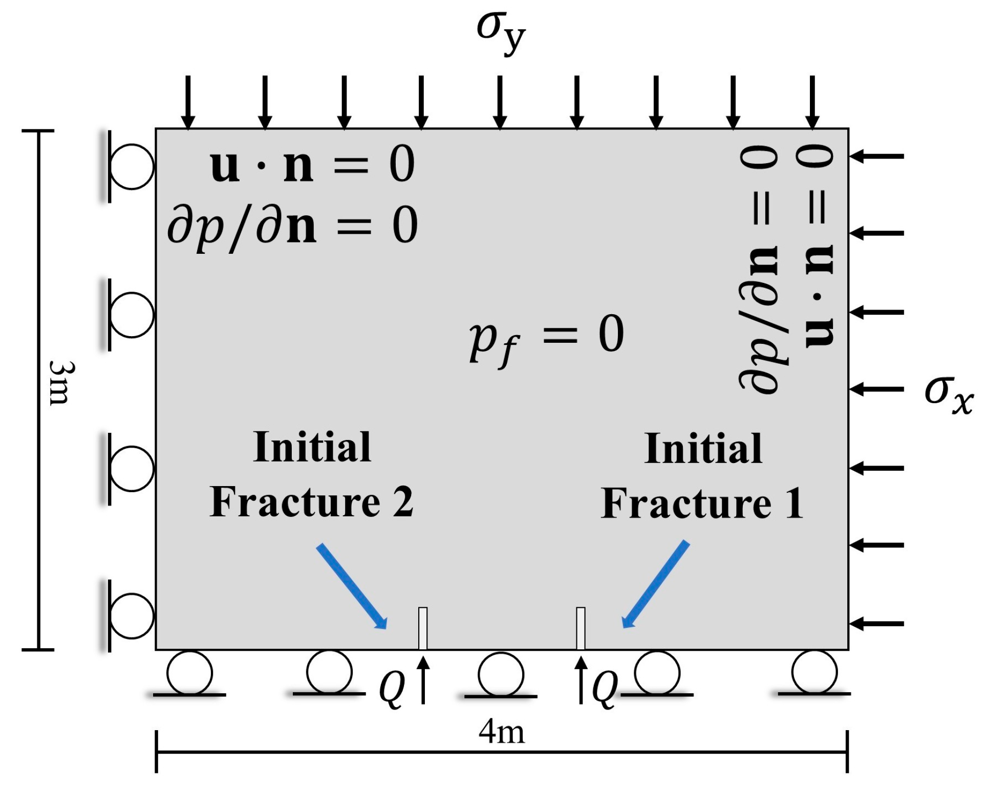
In this section, we present the phase-field model developed for simulating sequential fracturing, along with the corresponding simulation results. As shown in Figure 3, a two-dimensional computational model was established to represent the sequential fracturing process in a horizontal well. The total stimulation time for the simulation is set to 2$\mathrm{T}$, with each individual stimulation step lasting $\mathrm{T}$. In this region, fluid is injected sequentially into the two initial fractures at a constant injection rate. Horizontal and vertical confining stresses, ${\sigma }_x$ and ${\sigma }_y$ are applied along the respective directions. $p=0$ indicates zero-pressure condition applied at the boundaries, and $\mathbf{u}·\mathbf{n}=\mathbf{0}$ denotes a zero normal displacement component at the boundary, where $\mathbf{u}$ represents the displacement vector and $\mathbf{n}$ is the unit outward normal to the boundary.

To reduce computational cost, we assume that the fracture is fully filled with proppant after each stimulation step. First, we separately validate the evolution of fracture morphology in the case of single-fracture propagation and that under proppant support. Subsequently, a comparative analysis is conducted to investigate the morphological differences between fractures under various numerical models. Finally, a sensitivity analysis is conducted to evaluate the influence of dimensionless parameters on fracture geometry.

3.1. Validation of the Numerical Model

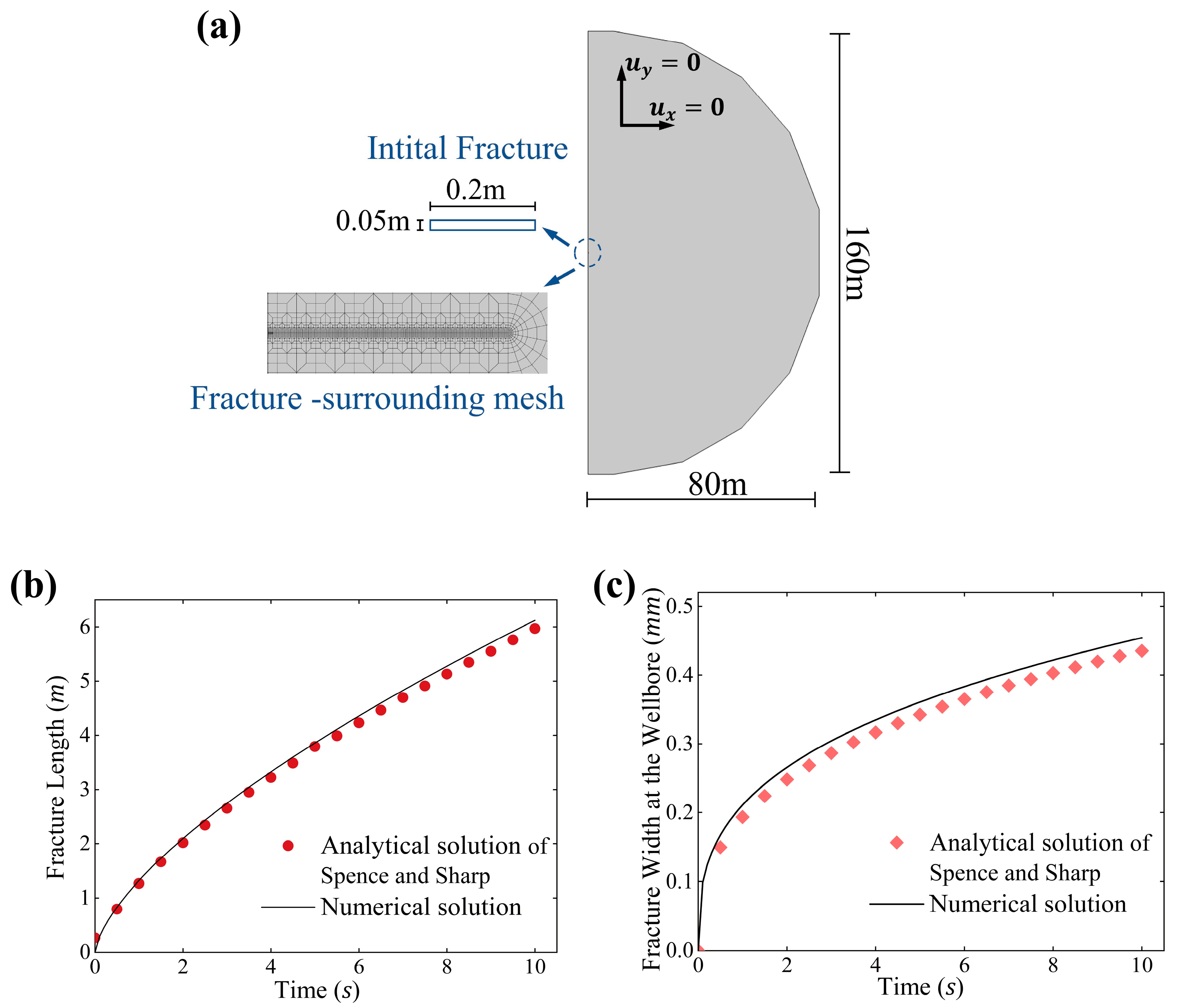
We use the asymptotic solutions of Spence and Sharp [54] to verify the feasibility of the phase-field model. The geometry of numerical model is shown in Figure 4a. The model consists of a semi-circular domain with a radius of 80 m. An initial fracture with a length of 0.2 m is placed at the center of the circle. The minimum mesh size is set to $h_e=0.05 \mathrm{m}$, The effect of in situ stress is neglected, and the specific model parameters are listed in

Table 1. Parameters for verification.

Parameter	Value	Unit
Young’s modulus $(E$)	$16$	$\mathrm{G}\mathrm{P}\mathrm{a}$
$\mathrm{Shear} \mathrm{modulus} (G$)	$6.2$	$\mathrm{G}\mathrm{P}\mathrm{a}$
$\mathrm{Poisson}’\mathrm{s} \mathrm{ratio} (\nu$)	$0.29$	—
$\mathrm{Porosity} (n$)	$0.19$	—
$\mathrm{Fluid} \mathrm{velocity} (\mathrm{v}$)	${4 \times 10}^{-3}$	$\mathrm{m}/\mathrm{s}$
$\mathrm{Flow} \mathrm{rate} (Q$)	${2 \times 10}^{-4}$	${\mathrm{m}}^2/\mathrm{s}$
$\mathrm{Fluid} \mathrm{density} (\rho$)	$1000$	$\mathrm{k}\mathrm{g}/{\mathrm{m}}^3$
$\mathrm{Fluid} \mathrm{viscosity} (\mu$)	${1 \times 10}^{-3}$	$\mathrm{P}\mathrm{a}·\mathrm{s}$
$\mathrm{Permeability} (k$)	${1 \times 10}^{-20}$	${\mathrm{m}}^2$
$\mathrm{Critical} \mathrm{energy} \mathrm{release} \mathrm{rate} (G_c$)	$20$	$\mathrm{N}/\mathrm{m}$
$\mathrm{Length} \mathrm{scale} (l_0$)	$0.2$	$\mathrm{m}$
$\mathrm{Minimum} \mathrm{mesh} \mathrm{size} (h_e$)	$0.05$	$\mathrm{m}$

. The temporal evolution of fracture length and fracture width at the wellbore during injection is provided in [55]:

$$l=0.65{\left[{\displaystyle \frac{G{Q}^3}{\left(1-\mathrm{v}\right)\mu }}\right]}^{{\displaystyle \frac{1}{6}}}{t}^{{\displaystyle \frac{2}{3}}}$$

(45)

$$w_a=2.14{\left[{\displaystyle \frac{\left(1-\mathrm{v}\right)\mu Q^3}{G}}\right]}^{{\displaystyle \frac{1}{6}}}{t}^{{\displaystyle \frac{1}{3}}}$$

(46)

The numerical results, shown in Figure 4b,c, exhibit excellent consistency with the analytical solutions in terms of both fracture length and width, verifying the accuracy of the proposed model.

In sequential fracturing simulations, it is a challenge to capture the fracture closure that follows proppant injection. This complex physical process involves intricate force interactions between the proppants and the fracture surfaces, making the accurate characterization of deformation behavior a long-standing challenge in the field.

In addition, we further validate the closure of the fracture surfaces induced by other fractures. Building upon the expression for the proppant-induced reaction stress ${\sigma }_p\left(w\right)$ given in Equation (31), a modified formulation can be derived to describe the variation in fracture width $w$ as a function of ${\sigma }_p\left(w\right)$:

$$w={\displaystyle \frac{{\sigma }_p\left(w\right)}{9{\sigma }_c+{\sigma }_p\left(w\right)}}{w}_{max}$$

(47)

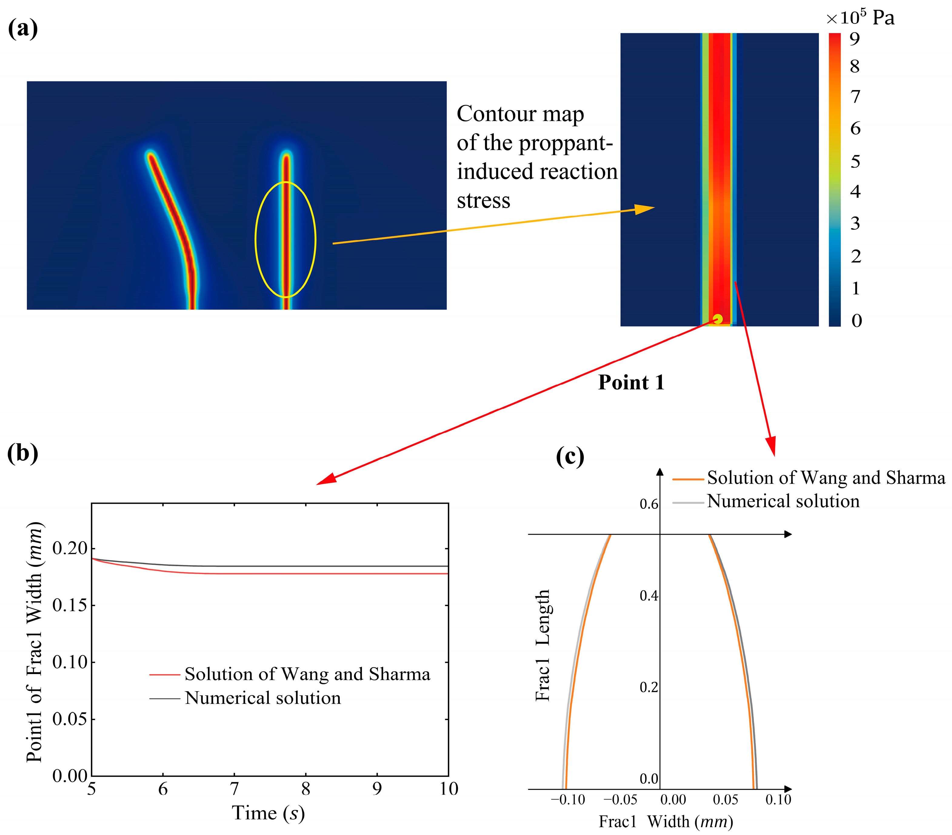
Figure 5 presents the validation results of the propped fracture morphology. Figure 5a shows the contour plot of the proppant-induced reaction stress in Frac 1 at time 2T after injecting proppant; Figure 5b illustrates the time evolution of fracture width at Point 1; Figure 5c illustrates fracture morphology at time 2$\mathrm{T}$ within the magnified region shown in Figure 5a. It can be observed that the simulated propped fracture morphology agrees well with the analytical results.

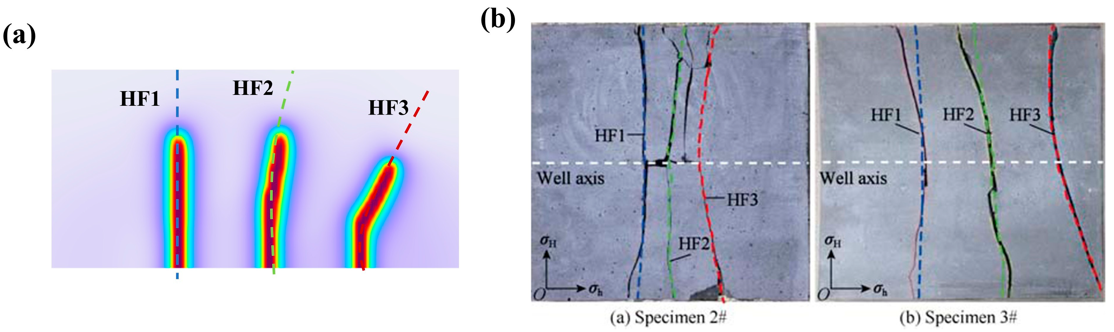
Furthermore, the propagation paths of the three fractures are compared with the experimental results reported by Liu et al. [56], as shown in Figure 6. Although the experimental and simulation conditions are not identical, our simulation of proppant-supported fractures serves as an equivalent representation of the constant net pressure in fractures maintained during the experiment. From a geomechanical perspective, both approaches exert a sustained internal force that inhibits fracture closure and sustains the induced stress field. The simulation results exhibit high consistency in terms of physical patterns with the experimental observations: as fractures are initiated sequentially, the horizontal stress induced by preceding fractures accumulates, leading to a trajectory where fracture 3 demonstrates a more pronounced outward deflection than fracture 2. This confirms the capability of our model to capture stress-driven interactions during sequential fracturing.

3.2. Mesh Sensitivity Analysis

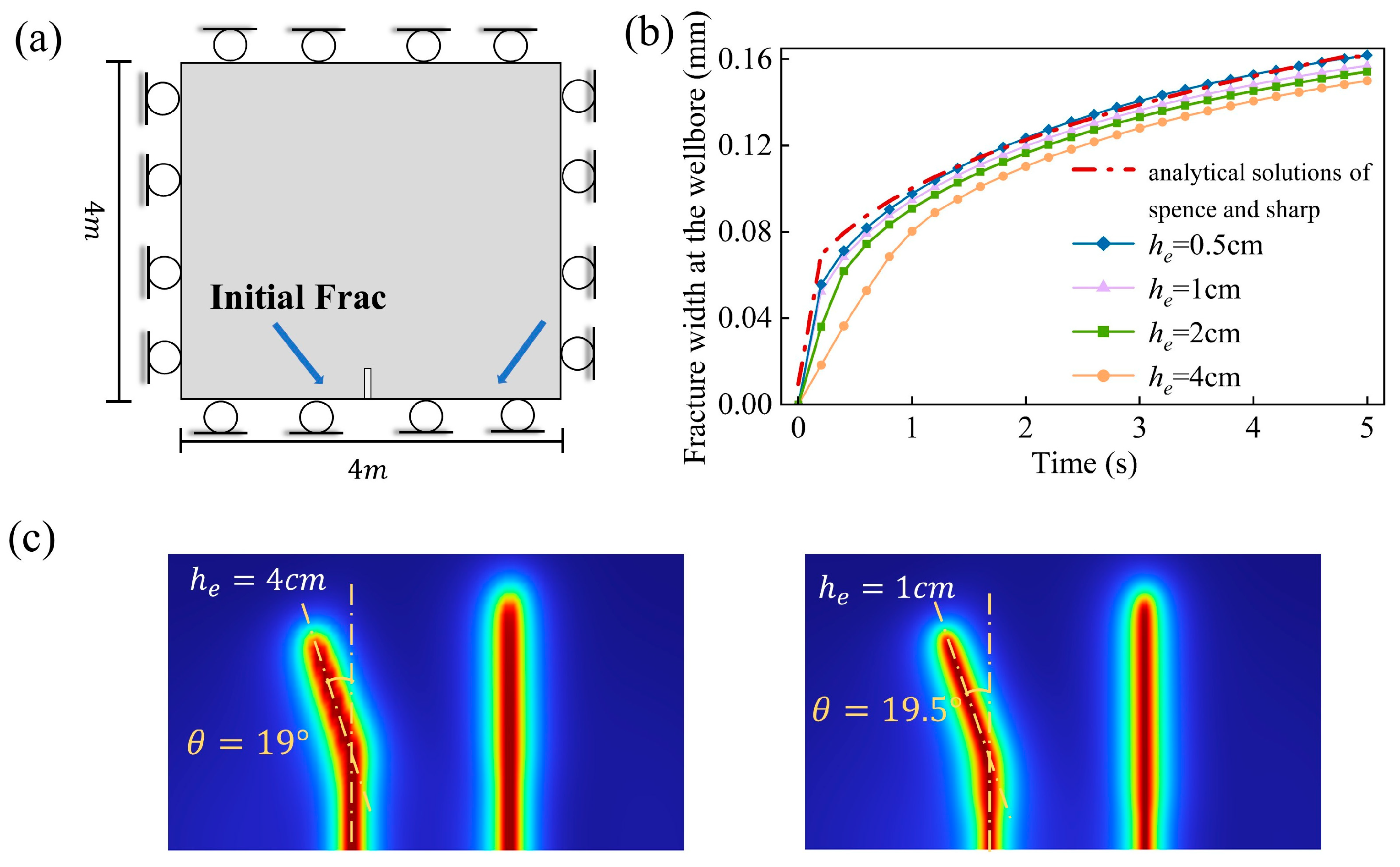
This section presents a mesh sensitivity analysis from two aspects: fracture width and fracture deflection. Since the calculated fracture width is sensitive to the mesh size, it is necessary to evaluate the influence of mesh resolution on the numerical results. In addition, due to the complex interactions between fractures during sequential fracturing, it is difficult to directly validate the results using analytical stress solutions. Therefore, the fracture deflection angle is introduced as an auxiliary metric, which reflects the evolution of the stress field during fracture propagation. As shown in Figure 7a, a $4\hspace{0.17em}\mathrm{m} \times 4\hspace{0.17em}\mathrm{m}$ computational model is established, with parameters consistent with those listed in Table 1. The total simulation time is $5 \mathrm{s}$. In the mesh sensitivity analysis, the minimum mesh size is varied, considering four cases of $4 \mathrm{c}\mathrm{m}$, $2 \mathrm{c}\mathrm{m}$, $1 \mathrm{c}\mathrm{m}$, and $0.5 \mathrm{c}\mathrm{m}$. The numerical results are compared with the analytical solution proposed by Spence and Sharp. The results indicate that when the mesh size is 4 cm, the average relative error between the numerical and analytical solutions is $15.8\%$. As the mesh size decreases, the numerical results gradually converge to the analytical solution. When the mesh size is reduced to $1 \mathrm{c}\mathrm{m}$, the average relative error decreases to $4.5\%$, and further decreases to $2.3\%$ for a mesh size of $0.5 \mathrm{c}\mathrm{m}$. Figure 7c shows the fracture propagation paths during sequential fracturing (the model setup is shown in Figure 3). By comparing the fracture geometries under different mesh sizes, it can be observed that the deflection path of the second fracture is nearly identical, indicating that the mesh size has a limited influence on the stress field distribution and fracture propagation path. Considering both computational accuracy and efficiency, a minimum mesh size of $1 \mathrm{c}\mathrm{m}$ is adopted in this study. For time integration, an adaptive time-stepping scheme based on the generalized-$\alpha$ method is employed. The time increment $∆t$ is automatically adjusted according to the convergence behavior and local error estimation, with an upper limit of $0.0025 \mathrm{s}$. This strategy allows smaller time steps to be used during rapid fracture propagation and significant stress variations, thereby accurately capturing the key physical processes while maintaining numerical stability.

3.3. Evolution of Fracture Geometries for Sequential Fracturing

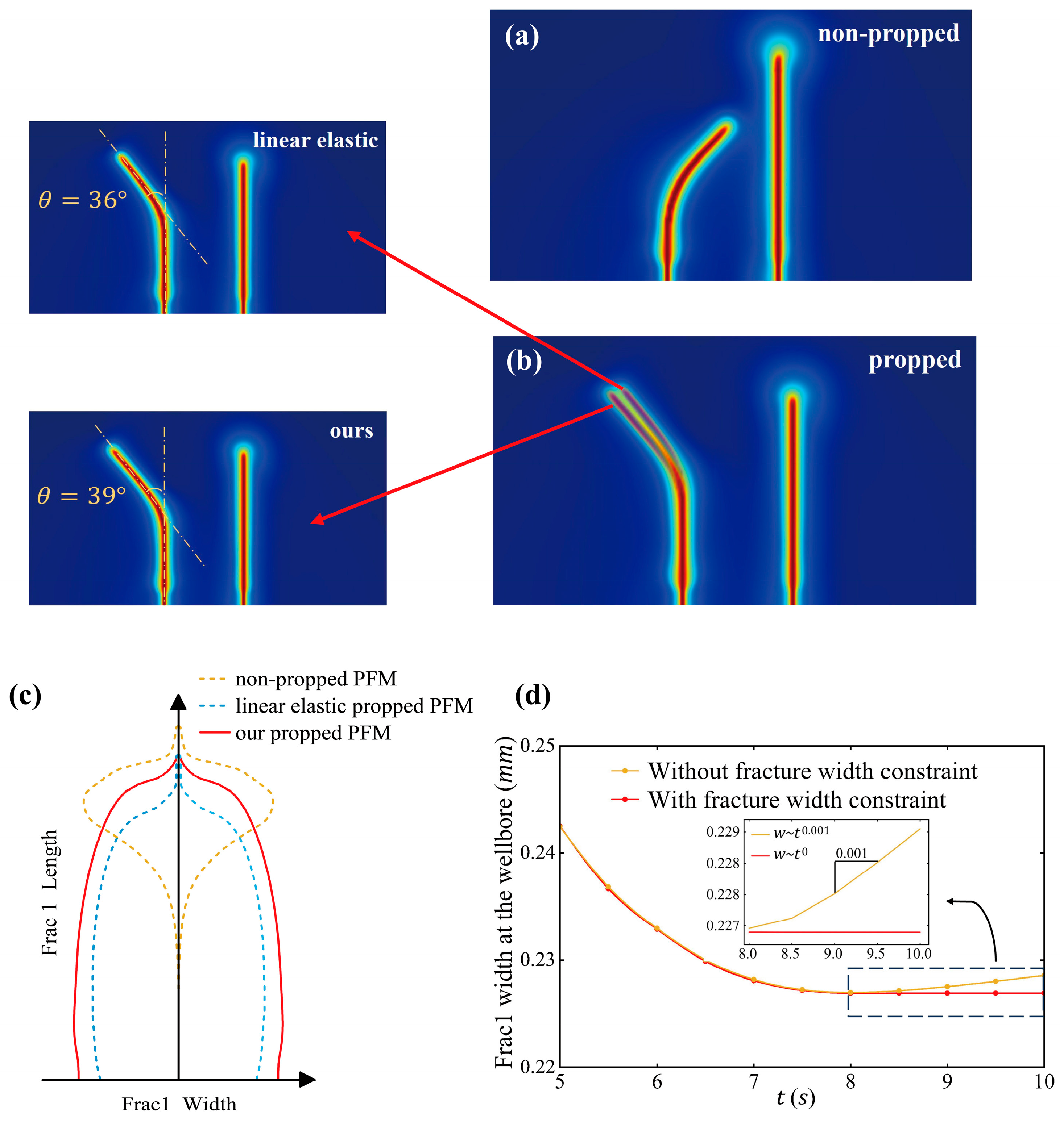
In this section, we investigate the evolution of the fracture geometries using the proposed sequential fracturing model. The closure of the propped fractures will be monotonically decreasing during stimulation process. To consider this effect, we introduce a constraint for the fracture width as shown in Equation (30). In Figure 8, two metrics are compared: fracture width and deflection angle. The deflection angle is the angular deviation from the initial perforation axis, evaluated at the final fracturing stage. It is measured by tracking the fracture’s main trajectory deviation from its initial direction using a digital geometric tool, ensuring consistency across simulations.

Figure 8a,b show the simulation results of sequential fracturing without and with proppant support, respectively. It is observed that, in the non-propped phase-field model, Frac 2 deflects toward Frac 1 primarily due to the lack of proppant support, which leads to significant fracture closure and consequently modifies the orientation of the principal stress. In contrast, in the propped PFM case, Frac 2 exhibits a noticeable outward deflection, which is attributed to the proppant-induced reaction stress generated during fracture closure and transmitted to Frac 2. Figure 8c compares the fracture geometries of Frac 1 at time 2$\mathrm{T}$ across different models. For non-propped PFM, significant closure occurs with increasing fluid pressure, which further promotes fracture propagation. Conversely, the propped PFM exhibits markedly different behavior—the presence of proppant effectively maintains both the width and length of Frac 1, preserving its initial geometry with minimal deformation. In addition, we compare the results obtained from the proposed model with those predicted by a linear elastic proppant–fracture interaction model that describes the reaction stress. The linear elastic model, applicable during fracture closure, is formulated as:

$${\sigma }_c={\displaystyle \frac{{\sigma }_p}{9}}\left({\displaystyle \frac{w_{max}-w}{w_{max}+k}}\right)$$

(48)

As shown in Figure 8b,c, simulations using the linear elastic propped PFM exhibit more pronounced fracture closure compared to those obtained with the proposed propped PFM. This discrepancy arises because the reaction force exerted by the proppant acts unidirectionally—only in compression against the fracture surfaces. In this study, we incorporate this physical constraint using Equation (30) to enforce unidirectional contact behavior. In contrast, conventional linear elastic models [36] do not account for this effect. To investigate the influence of constraining fracture width on simulation results, we compare cases with and without this constraint. Figure 8d compares the fracture width evolution of Frac 2 between the standard phase-field model and the present formulation of time-dependent width constraint through Equation (30). In the unconstrained case (yellow curve), the fracture width increases again after entering the closure stage ($\mathrm{w}\sim {\mathrm{t}}^{0.001}$). This phenomenon arises from the fact that the fluid pressure within the fracture continues to act on the fracture surfaces during closure in the standard phase-field formulation. However, such secondary opening is rarely observed in practice, where fracture closure is dominated by mechanical contact and proppant resistance. To address this issue, a width constraint is introduced to constrained closure. This treatment effectively suppresses the nonphysical reopening and results in a nearly constant fracture width during the late stage ($\mathrm{w}\sim {\mathrm{t}}^0$), which is more consistent with engineering observations. It is important to note that this constraint is not a universal physical law, but rather a specific formulation designed for the monotonic loading or sequential fracturing scenarios studied in this work. In more complex loading paths, such as cyclic loading or stress reversal, more intricate fracture behavior may occur, and this simplified approach may no longer be valid. As such, further investigation is required to improve the physical representation of fracture behavior under these more complex loading conditions.

Although the deflection angles and fracture widths show only minor differences between the different propped PFM approaches, these small discrepancies become progressively amplified during sequential fracturing operations. As the number of fracturing steps increases, the cumulative effect can lead to substantial deviations in predicted fracture trajectories, significantly impacting the accuracy of multi-step hydraulic fracturing simulations in horizontal wells. The proposed model in this study effectively addresses these two sources of inaccuracy—inaccurate proppant-induced reaction forces and the lack of unidirectional constraints—thereby further enhancing the predictive capability of fracture propagation in complex, multi-step scenarios.

3.4. Dimensional Analysis

Main parameters that affect the fracture geometries are presented in Table 1. Additional supplementary parameters, such as the in situ stress difference, are also taken into account. Dimensional analysis leads to a reduction in the number of parameters. This simplification facilitates a more efficient investigation into the relationships between model parameters and fracture characteristics, such as the deflection angle $\theta$ and fracture width $w$. Based on Xie et al. [57], we comprehensively selected the following parameters that may affect fracture deflection, including the fracture spacing $d$, the length $l$ of Frac 1, the elastic modulus $E$ of the rock, the rock fracture energy release rate $G_c$, the injection rate $\mathrm{v}$ and kinematic viscosity $\upsilon$ of the fracturing fluid, the differential horizontal in situ stress $∆\sigma$ ($∆\sigma ={\sigma }_y-{\sigma }_x)$, and the contact reference stress ${\sigma }_p$ of proppant pack.

According to the $\pi$-theorem of dimensional analysis, the relationship between the deflection angle $\theta$ of Frac 2 and the aforementioned eight parameters can be expressed as follows:

$$F\left(\theta ,d,l,E,G_c,\mathrm{v},\upsilon ,∆\sigma ,{\sigma }_p\right)=0$$

(49)

For the hydraulic fracturing problem, it is necessary to select a set of mutually independent parameters that span the fundamental dimensions of length ($L$), time ($T$), and mass ($M$) as the base quantities. We selected the length of Frac 1, $l$($L$); the injection velocity of fracturing fluid, $\mathrm{v}$($L{T}^{-1}$); and the elastic modulus of the rock $E$($M{L}^{-1}{T}^{-2}$) are chosen as three independent base parameters. The remaining parameters are then transformed into a set of dimensionless groups as follows:

$${\displaystyle \frac{\upsilon }{\mathrm{v}l}}={\displaystyle \frac{L^2{T}^{-1}}{\left(L{T}^{-1}\right)\left(L\right)}}=1$$

(50a)

$${\displaystyle \frac{G_c}{El}}={\displaystyle \frac{M{T}^{-2}}{\left(M{L}^{-1}{T}^{-2}\right)\left(L\right)}}=1$$

(50b)

$${\displaystyle \frac{∆\sigma }{E}}={\displaystyle \frac{M{L}^{-1}{T}^{-2}}{M{L}^{-1}{T}^{-2}}}=1$$

(50c)

$${\displaystyle \frac{d}{l}}={\displaystyle \frac{L}{L}}=1$$

(50d)

$${\displaystyle \frac{{\sigma }_p}{E}}={\displaystyle \frac{M{L}^{-1}{T}^{-2}}{M{L}^{-1}{T}^{-2}}}=1$$

(50e)

leading to the following final dimensionless formulation:

$$\theta =F_1\left(\upsilon /vl,G_c/El,∆\sigma /E,d/l,{\sigma }_p/E\right)$$

(51)

As indicated by Equation (51), the deflection angle $\theta$ is related to five dimensionless parameters, each of which carries distinct physical significance. The parameter $\upsilon /\mathrm{v}l$ is inversely proportional to the Reynolds number $Re$ [58], characterizing the competition between viscous dissipation and inertial effects within the fracture fluid. The ratio $G_c/El$ represents the intrinsic material characteristic length relative to the actual fracture scale, reflecting the competition between energy dissipation and elastic deformation during fracture propagation. The parameter $∆\sigma /E$ represents the characteristic strain induced by the differential in situ stress relative to the rock stiffness. It quantifies the external tectonic driving force that interacts with the rock’s elastic and fracture resistance, thereby influencing the fracture deflection angle. The parameter $d/l$, defined as the ratio of fracture spacing $d$ to fracture length $l$, characterizes the degree of interaction between adjacent fractures. Since $d$ governs the intensity of the stress shadowing effect and $l$ reflects the spatial extent of influence of an individual fracture, the $d/l$ ratio serves as an indicator of the extent to which stress shadowing affects the fracture deflection angle. Lastly, in the parameter ${\sigma }_p/E$, ${\sigma }_p$ denotes the contact reference stress for the proppant pack, while $E$ is the elastic modulus. This ratio reflects the fracture’s resistance to closure after hydraulic fracturing and, therefore, indicates the ability of Frac 1 to remain open following the completion of the fracturing operation.

We defined a specific range for each dimensionless parameter for the purpose of sensitivity analysis, as shown in

Table 2. Numerical model parameters.

Parameter	Value	Unit
$\upsilon /\mathrm{v}l$	${3.03 \times 10}^2~{6.06 \times 10}^2$	—
$G_c/El$	${9.48 \times 10}^{-9}~{1.89 \times 10}^{-8}$	—
$∆\sigma /E$	$0~{9.38 \times 10}^{-5}$	—
$d/l$	$0.76~1.9$	—
${\sigma }_p/E$	${3.10 \times 10}^{-3}~{1.88 \times 10}^{-1}$	—
Poisson’s ratio ($\nu$)	$0.29$	—
Porosity ($n$)	$0.19$	—
Permeability ($k$)	${1 \times 10}^{-20}$	${\mathrm{m}}^2$
Per-step time ($T$)	5	$\mathrm{s}$

. In addition, the values of several other parameters are also presented in Table 2. The range of ${\sigma }_p$ is set between $0.1 \mathrm{G}\mathrm{P}\mathrm{a}$ and $3 \mathrm{G}\mathrm{P}\mathrm{a}$, with higher values indicating a greater resistance to fracture closure.

The reservoir physical parameters used in Table 2 are selected based on the representative ranges typical of shale and tight formations. Specifically, the differential stress ($0–2 \mathrm{M}\mathrm{P}\mathrm{a}$) represents weak to moderate in situ stress contrasts commonly encountered in horizontal well fracturing. The elastic modulus ($12–16 \mathrm{G}\mathrm{P}\mathrm{a}$) falls within the typical range for shale formations (approximately $10–30 \mathrm{G}\mathrm{P}\mathrm{a}$), indicating moderate rock stiffness. The porosity (0.19) falls within the typical range of shale reservoirs (generally 0.05–0.20), and is characteristic of organic-rich formations with relatively well-developed pore structures. The Poisson’s ratio (0.29) lies within the commonly reported range for shale (0.2–0.35), reflecting typical elastic deformation behavior. The permeability ($1\times {10}^{–20}{\mathrm{m}}^2$) is representative of ultra-low permeability conditions in tight reservoirs (typically ${10}^{-21}-{10}^{-18} {\mathrm{m}}^2$). Therefore, the selected parameter values ensure that the simulation conditions are physically representative of realistic shale/tight reservoir environments.

3.5. Effect of Dimensionless Parameters on Deflection Angle

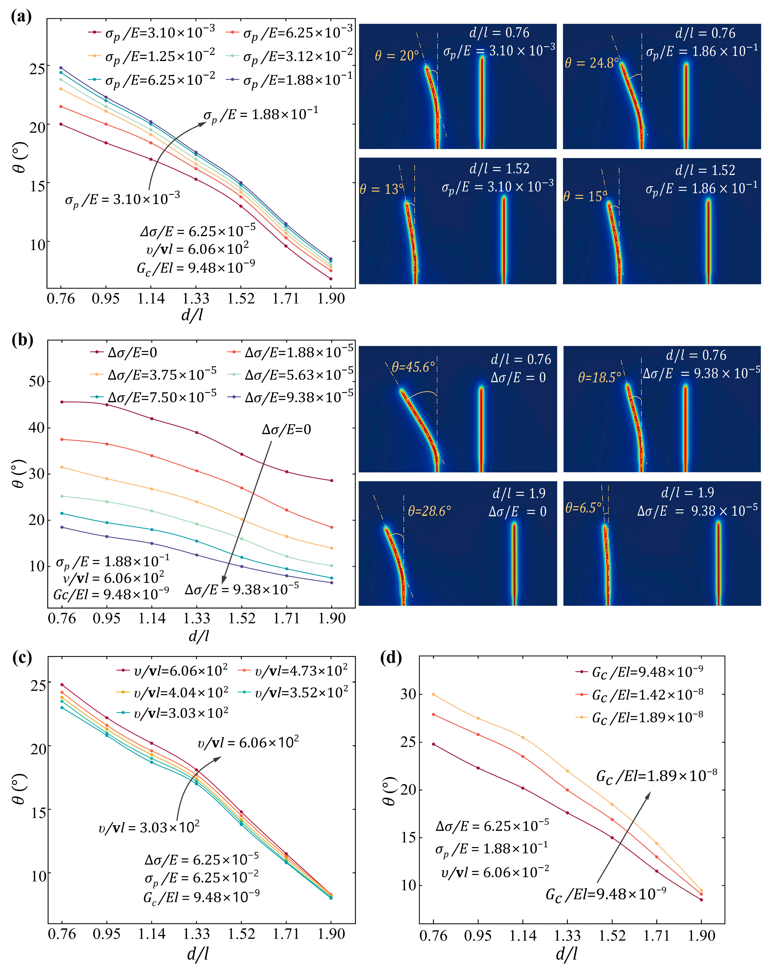
Based on the parameter ranges listed in Table 2, multiple simulations were conducted to investigate the relationship between the dimensionless parameters and the deflection angle, as illustrated in Figure 9. $d/l$ was chosen as the $x$-axis, while the deflection angle was taken as the $y$-axis. By varying each of the other four dimensionless parameters, the influence of all five parameters including $d/l$ on the deflection angle was systematically examined. As shown in Figure 9a–d, a negative correlation is observed between $\theta$ and $d/l$. A smaller value of $d/l$ indicates stronger interactions between neighboring fractures, which leads to an increase in the deflection angle $\theta$. In Figure 9a, a positive correlation between ${\sigma }_p/E$ and $\theta$ can be observed. An increase in ${\sigma }_p/E$ implies a higher ratio of reference contact stress of the proppant pack to rock stiffness, which leads to a larger deflection angle. In Figure 9b, a negative correlation between $∆\sigma /E$ and $\theta$ can be observed. An increase in $∆\sigma /E$, representing a higher ratio of differential horizontal in situ stress to rock stiffness, indicates that the fracture tends to propagate more easily along the ${\sigma }_y$ direction, leading to a smaller deflection angle. In Figure 9c, $\upsilon /\mathrm{v}l$ exhibits a negative correlation with $\theta$. The dimensionless parameter $\upsilon /\mathrm{v}l$ can be approximately regarded as the inverse of the Reynolds number $Re$. As $Re$ increases, $\upsilon /\mathrm{v}l$ decreases, leading to a larger deflection angle. In Figure 9d, $G_c/El$ shows a positive correlation with $\theta$. The parameter $G_c/El$ reflects the intrinsic mechanical properties of the rock. As $G_c/El$ increases, the deflection angle $\theta$ also increases.

By synthesizing the results from Figure 9a–d, the sensitivity of the five dimensionless parameters to the deflection angle $\theta$ can be ranked in descending order as follows: $d/l$, $∆\sigma /E$, ${\sigma }_p/E$, $G_c/El$ and $\upsilon /\mathrm{v}l$. Among them, ${\sigma }_p/E$ and $G_c/El$ exhibit a positive correlation with the deflection angle $\theta$, while $d/l$, $∆\sigma /E$ and $\upsilon /\mathrm{v}l$ show a negative correlation with the deflection angle.

Considering the limitation that the aforementioned analytical approach cannot capture parameter interaction effects, this study further introduces a systematic quantitative sensitivity analysis framework. A Ridge regression surrogate model [59] incorporating second-order interaction terms is constructed based on dimensionless parameters, thereby enabling a unified evaluation of both the main effects of individual parameters and their pairwise interactions. On this basis, the Morris method [60,61] is employed to conduct a global sensitivity analysis. This method evaluates the contribution of each parameter by calculating its elementary effects, which are defined as follows:

$$E{E}_i={\displaystyle \frac{f\left(x_1,\dots ,x_i+∆,\dots ,x_5\right)-f\left(x\right)}{∆}}$$

(52)

here, $x_1~x_5$ denote the five corresponding dimensionless parameters, and $x_i$ represents the (i)-th parameter. The function $f\left(·\right)$ denotes the mapping established by the surrogate model, which is used to compute the system response output, while $∆$ represents the sampling step size in the parameter space. The elementary effect $E{E}_i$ reflects the local rate of change in the system output induced by varying parameter $x_i$ alone, while keeping all other parameters fixed. To further characterize the sensitivity, two statistical measures are employed. The average effect μ^* is used to quantify the overall importance of each parameter, and is defined as follows:

$${\mu }_i={\displaystyle \frac{1}{N}}{\sum }_{j=1}^N\left|E{E}_{i,j}\right|$$

(53)

Here, j denotes the j-th sampling trajectory generated by the Morris method in the input space, and N is the total number of trajectories. Each trajectory can be regarded as an experiment in which individual parameters are perturbed sequentially under a specific parameter background, while all other parameters remain fixed. By repeating this process across multiple randomly sampled backgrounds, the algorithm is able to achieve comprehensive coverage of the parameter space. This metric evaluates the overall importance of parameter $x_i$ by taking the mean of the absolute values of the elementary effects over all trajectories. The standard deviation $\sigma$ is used to quantify the variability of the elementary effects $E{E}_{i,j}$ across different sampling trajectories, thereby reflecting the degree of nonlinearity in the influence of parameter $x_i$ on the system response, as well as potential interaction effects. It is defined as follows:

$${\sigma }_i=\sqrt{{\displaystyle \frac{1}{N-1}}{\sum }_{j=1}^N{\left(E{E}_{i,j}-{\mu }_i\right)}^2}$$

(54)

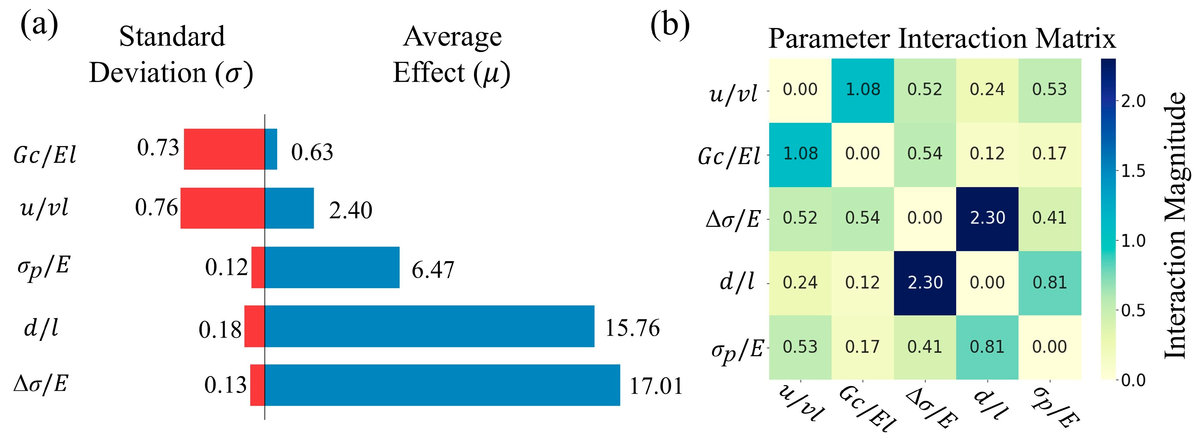
It should be noted that, owing to the high computational cost of the model, the surrogate model in this study is constructed based on only 36 sample datasets. However, since the primary objective of this work is to identify the underlying influence patterns of the parameters rather than to achieve highly accurate quantitative predictions, such a sample size is considered sufficient. Moreover, the incorporation of cross-validation and regularization techniques further ensures the stability and generalization capability of the model. As shown in Figure 10a, the results indicate that parameters $∆\sigma /E$ and $d/l$ exhibit significantly higher μ^* values than the other parameters, suggesting that they play a dominant role in the system response. Although the μ^* value of parameter ${\sigma }_p/E$ is slightly lower than those of $∆\sigma /E$ and $d/l$, it remains markedly higher than that of the remaining parameters, indicating that it serves as a secondary yet still important influencing factor. In contrast, $\upsilon /\mathrm{v}l$ and $G_c/El$ show relatively low μ^* values accompanied by relatively large $\sigma$, implying that their effects on the system are primarily manifested through interactions with other parameters rather than through independent contributions. Furthermore, the interaction coefficients extracted from the Ridge model and the constructed interaction matrix indicate a pronounced interaction between $∆\sigma /E$ and $d/l$, with a strength significantly greater than that of other parameter combinations. Meanwhile, the interactions between $\upsilon /\mathrm{v}l$ and $G_c/El$, as well as between $d/l$ and ${\sigma }_p/E$, although present, are comparatively weaker. These results suggest that the system behavior is governed not only by the main effects of individual parameters but also by the underlying interactions among them. This finding also provides a useful direction for more in-depth parametric investigations in future studies.

In summary, the significantly higher ${\mu }^{*}$ values and relatively small $\sigma$ of $∆\sigma /E$ and $d/l$ indicate that these parameters exert a stable and pronounced influence on the system response. Meanwhile, although ${\sigma }_p/E$ is of secondary importance, it still plays a non-negligible role in the system.

3.6. Effect of Dimensionless Parameters on Frac 1 Morphology

During sequential hydraulic fracturing, the initiation of Frac 2 induces horizontal stresses on the previously created Frac 1 due to the fluid pressure within Frac 2, which promotes its closure. The deflection angle $\theta$ of Frac 2 governs the spatial extent of its stress shadow, and thus influences the stresses exerted on Frac 1. As a result, this affects the closure behavior of Frac 1, indicating that the dimensionless parameters discussed earlier are also linked to the final width of Frac 1. To further analyze the influence of these parameters on the fracture morphology, we selected the dimensionless parameters that have a significant influence on the deflection angle $\theta$, namely $d/l$, $∆\sigma /E$ and ${\sigma }_p/E$ while $\upsilon /\mathrm{v}l$ and $G_c/El$ are fixed at ${3.03 \times 10}^2$ and ${9.48 \times 10}^{-9}$, respectively. Then, we analyzed the relationship between these parameters and the final f morphology of Frac 1 $w_{e,1}$. 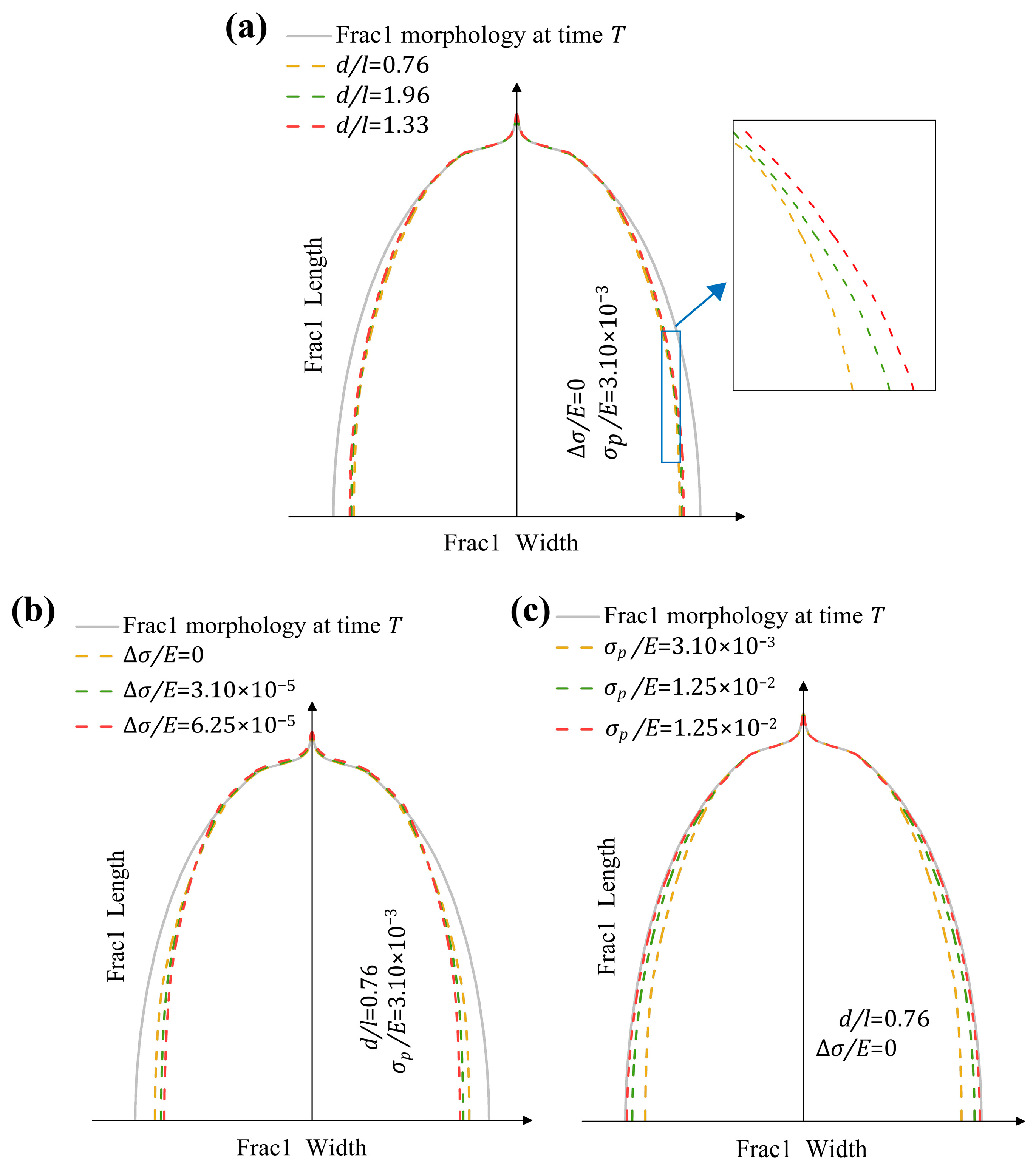As shown in Figure 11a, by keeping all parameters constant except for $d/l$, the variations in $w_{e,1}$ are compared. The solid line indicates the fracture morphology at the end of the first-step fracturing, which also serves as the initial moment for the second-step fracturing (Figure 11b,c follow the same setting as in Figure 11a). Figure 11b presents the changes in $w_{e,1}$ for different values of $∆\sigma /E$. An increase in $∆\sigma /E$ leads to greater fracture closure compared to the distribution at the initial time. Figure 11c shows how $w_{e,1}$ changes with varying ${\sigma }_p/E$. A higher ${\sigma }_p/E$ results in less closure compared to the width distribution at the initial time. However, the results shown in Figure 11a exhibit a different trend. As illustrated in the magnified view, the closure of Frac 1 does not exhibit a monotonic relationship with $d/l$. This is because the stress exerted on Frac 1 by Frac 2 depends not only on the dimensionless parameter $d/l$, but is also strongly influenced by the deflection angle $\theta$ of Frac 2. In general, larger values of $d/l$ and $\theta$ result in weaker stress interactions on Frac 1. As $d/l$ increases, the stress shadowing effect generally decreases. However, the reduction in $\theta$ with increasing $d/l$ may enhance the stress shadowing effect to an extent that outweighs the overall decrease in its magnitude. This suggests the existence of a critical $d/l$ value. Beyond this threshold, the variation in $\theta$ becomes less significant, and instead, the $w_{e,1}$ begins to increase steadily as $d/l$ decreases.

3.7. Effect of Dimensionless Parameters on Frac 2 Morphology

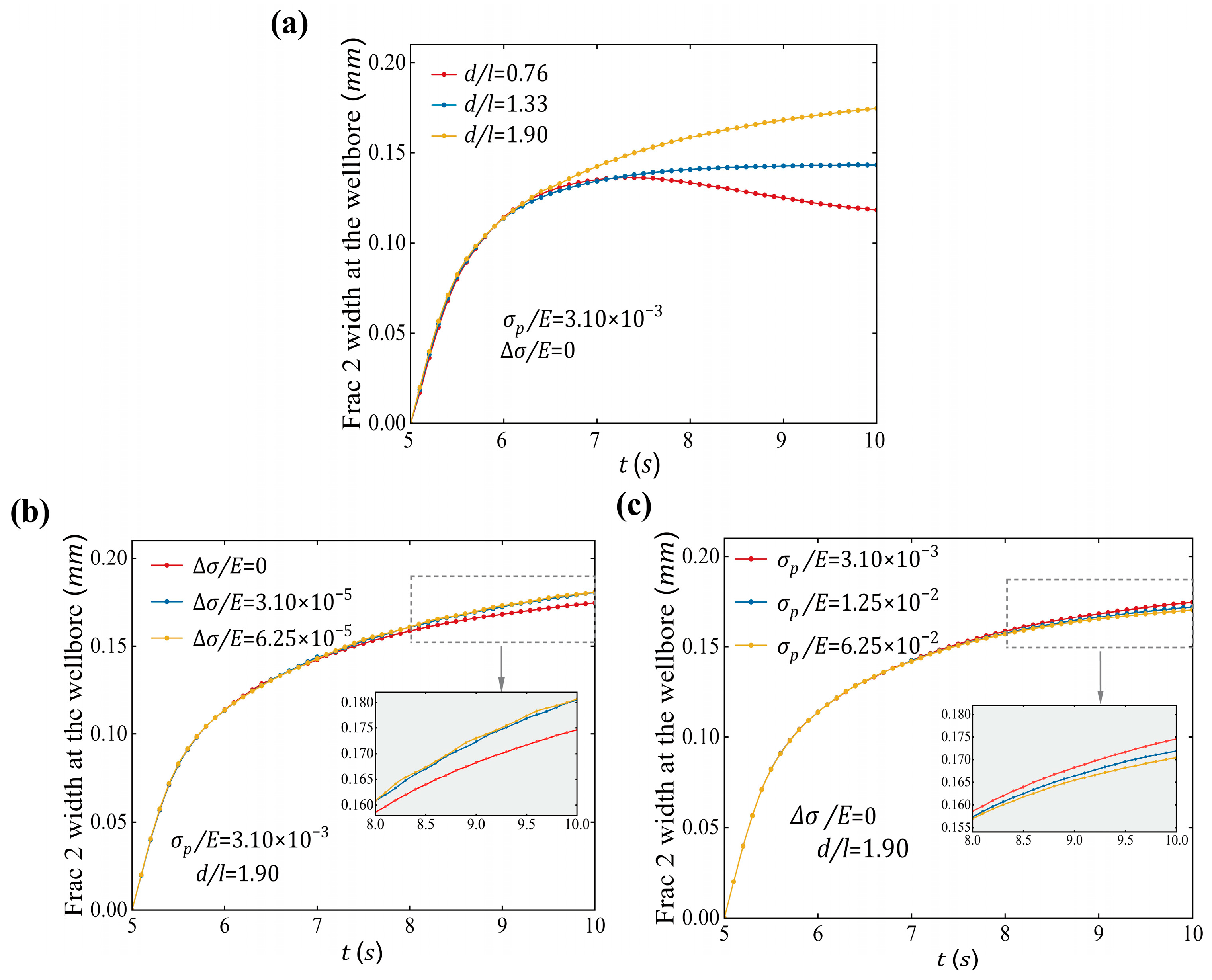
The influence of these parameters on the morphology of Frac 2 was examined. The fracture morphology is characterized by the fracture width at the wellbore, $w_{w,2}$, which effectively represents the overall trend of fracture width evolution. Figure 12 illustrates the variation trend of $w_{w,2}$ about changes in the dimensionless parameters. The analysis focuses on the same set of parameters: $d/l$, $∆\sigma /E$ and ${\sigma }_p/E$, while $\upsilon /\mathrm{v}l$ and $G_c/El$ are fixed at ${3.03 \times 10}^2$ and ${9.48 \times 10}^{-9}$, respectively. As shown in Figure 12a, the increase in $d/l$ leads to a gradual reduction in the growth rate of $w_{w,2}$. Similarly, Figure 12b indicates that an increase of $∆\sigma /E$ also leads to a slower growth of $w_{w,2}$ after 6.5 s. In contrast, as shown in Figure 12c, an increase in ${\sigma }_p/E$ results in an enhanced late-step growth trend of $w_{w,2}$. Before 6.5 s, the growth curves under different conditions are nearly identical across all three subfigures. This is because, during the early step of the second-step fracturing, the closure of Frac 1 is relatively minor, resulting in limited proppant-induced reaction stress and thus a minimal influence on Frac 2. As the closure of Frac 1 increases, the reaction stress also rises. Under a stronger stress interference, the effects of the dimensionless parameters are amplified, leading to more pronounced differences. Consistent with the previous analysis of the effects of dimensionless parameters, a smaller $d/l$ or $∆\sigma /E$, or a larger ${\sigma }_p/E$ all lead to a greater deflection angle of Frac 2. This, in turn, indicates stronger stress interactions between the two fractures, ultimately resulting in a lower value of $w_{w,2}$. A downward trend is observed in the red curve of Figure 12a during the later steps, which may indicate a slight deviation from the expected behavior. This is because the reaction stress increases progressively as the fracture closes. When the value of $d/l$ is relatively low, the stress interaction between the fractures becomes more significant. Once the reaction stress acting on Frac 2 exceeds its internal fluid pressure, slight fracture closure occurs.

3.8. Proppant–Fracture Interaction Model for Nonplanar Fractures

Moreover, in the three-step fracturing process, the spatial and temporal ranges of the proppant-induced reaction stress for Frac 1 and Frac 2 are different. Therefore, further refinement is required to accurately describe the proppant-supported closure stress of the two fractures:

$${\sigma }_{c,1}\left(w\right)={\displaystyle \frac{{\sigma }_p}{9}}{D}_{proppant}{\displaystyle \frac{w_{1,max}-w_1}{w_1+k}}H\left(x_{{\Omega }_{Frac1}}\right)H\left(t-T\right) \left(\Omega ϵ{\Omega }_{Frac1}\right)$$

(55a)

$${\sigma }_{c,2}\left(w\right)={\displaystyle \frac{{\sigma }_p}{9}}{D}_{proppant}{\displaystyle \frac{w_{2,max}-w_2}{w_2+k}}H\left(x_{{\Omega }_{Frac 2}}\right)H\left(t-2T\right) \left(\Omega ϵ{\Omega }_{Frac 2}\right)$$

(55b)

here, ${\sigma }_{c,1}\left(w\right)$ and ${\sigma }_{c,2}\left(w\right)$ denote the closure stresses of Frac 1 and Frac 2, respectively, after the injection of proppant. The global closure stresses can be expressed as:

$${\sigma }_c={\sigma }_{c,1}+{\sigma }_{c,2}$$

(56)

In this simulation, each fracturing step T lasts for 5 s. The material and fluid parameters are taken from Table 2. The dimensionless parameters ${\sigma }_p/E$, $∆\sigma /E$, $\upsilon /\mathrm{v}l$ and $G_c/El$ are fixed at ${1.88 \times 10}^{-1}$, ${6.25 \times 10}^{-5}$, ${3.03 \times 10}^2$ and ${9.48 \times 10}^{-9}$, respectively. Parameters $d_1$ and $d_2$ represent the spacing between Frac 1 and Frac 2, and between Frac 2 and Frac 3, respectively. Similarly, ${\theta }_1$ and ${\theta }_2$ denote the deflection angles of Frac 2 and Frac 3, respectively. We investigated how $d_2$ and ${\theta }_1$ influence ${\theta }_2$.

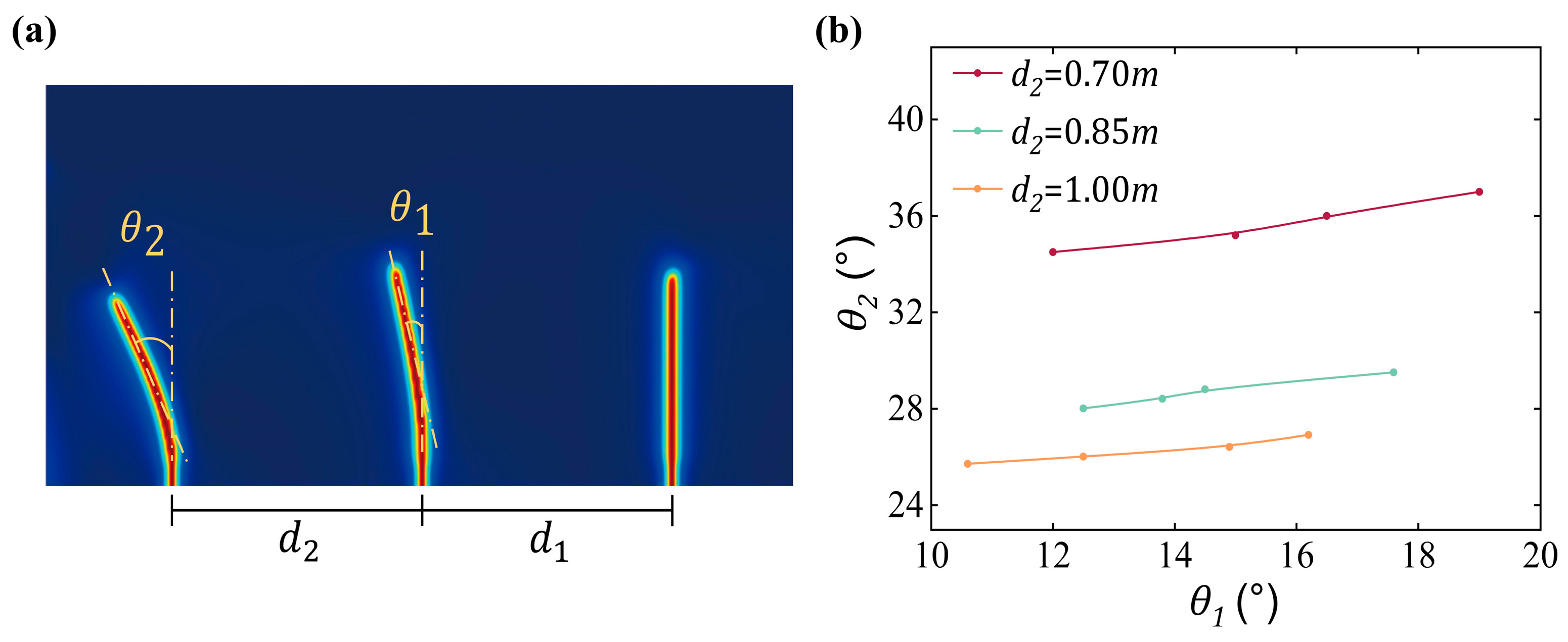
As shown in Figure 13, under fixed spacing conditions, an increase in ${\theta }_1$ leads to a corresponding increase in ${\theta }_2$. This observation is consistent with engineering practice. However, the influence of ${\theta }_1$ on ${\theta }_2$ is significantly weaker compared to that of $d_2$. The figures reveal that when $d_2$ increases from 0.5 m to 0.75 m, the deflection angle ${\theta }_2$ of Frac 3 changes by approximately $2°$. When $d_2$ further increases from 0.75 m to 1.0 m, the angle changes by about $6°$. This behavior is primarily attributed to the horizontal stresses induced by proppant during fracture closure. As the number of fractures increases, these stresses accumulate, leading to progressively larger deflection angles in subsequently formed fractures. Moreover, this stress effect is strongly distance-dependent: as the spacing increases, the stress interaction weakens, resulting in a corresponding reduction in fracture deflection. The stress effect is progressively amplified as the number of fractures increases. Therefore, accounting for proppant effects is essential for understanding fracture propagation paths in multi-stage sequential fracturing. The nonlinear response is more complex than that observed in the two-step case, indicating that parameter interactions in three-step or multi-step fracturing involving propped, nonplanar fractures are significantly more intricate. These findings point to an important direction for future research.

4. Conclusions

In this study, a phase-field-based numerical model was developed to simulate fracture propagation during sequential fracturing. The model incorporates a strain-based formulation to compute fracture width and accounts for the mechanical support provided by proppants through the calculation of their reaction stress, thereby more accurately representing real-world engineering conditions. In addition, the unexpected growth of previous fractures induced by stress shadowing is numerically solved. The fracture aperture and length versus injection time predicted by the proposed model were validated against the solution of Spence and Sharp [54]. Moreover, the numerically simulated fracture closure on proppant coincides with an analytical solution. The model’s capability to simulate sequential fracturing was demonstrated through a series of case studies. The proposed approach is validated for sequential fracturing in this study and may serve as a basis for future investigations into other fracturing strategies, such as staggered and zipper fracturing [62,63].

Dimensional analysis was performed on key parameters to assess their sensitivity with respect to fracture morphology. The effects of key dimensionless parameters on fracture deflections and widths were systematically investigated. Our results indicate that the dimensionless groups $d/l$ and $∆\sigma /E$ exhibit a negative correlation with the fracture deflection angle, whereas ${\sigma }_p/E$, $\upsilon /\mathrm{v}l$ and $G_c/El$ show a positive correlation. Among these, $d/l$, $∆\sigma /E$ and ${\sigma }_p/E$ exert the most significant influence on the deflection angle. Building on the analysis of these three most influential parameters, we found that their effects on the width of Frac 1 are consistent with their influence on the deflection angle of Frac 2. In contrast, their effects on the width of Frac 2 are opposite. This discrepancy emphasizes the vital role of proppant affecting the geometry of hydraulic fractures. Finally, we extended the reaction stress formula of the proppant into nonplanar fractures, and therefore, it can be applied in an arbitrary number of sequential fracturing steps. These results provide an effective numerical model for simulating sequential fracturing in horizontal wells and offer valuable insights into the interactions between hydraulic fractures. However, the current study is conducted within a 2D framework and assumes a uniform proppant distribution, neglecting complex transport processes and out-of-plane effects. These simplifications represent an idealized scenario where conclusions are primarily applicable to plane-strain conditions, and potential deviations may occur under realistic 3D field environments. In the future, the proposed model can be further extended into a 3D framework and integrated with proppant transport mechanisms. This evolution will capture the dynamic coupling between slurry flow, fracture evolution, and out-of-plane effects, providing a more comprehensive understanding of asymmetric proppant distribution and its long-term impact on sequential fracturing in realistic reservoir conditions.