Causal Learning for Continuous Variables with an Improved Bayesian Network Constructed by Symmetric Kernel Function Acceleration

Abstract

Bayesian network-based causal structure learning provides an effective framework for uncovering causal relationships among continuous variables. However, many existing methods for continuous data still rely on strong parametric distribution assumptions, which may introduce information loss and reduce Bayesian network modeling accuracy. Kernel density estimation (KDE), a non-parametric statistical method that is more flexible in density estimation form, offers a versatile framework for conducting conditional independence (CI) tests. This approach enables the estimation of mutual information and conditional mutual information, thereby facilitating the identification of underlying structural relationships. Nevertheless, the high computational cost of KDE-based CI testing restricts its practical application in continuous-variable causal learning. To address this issue, this study introduces a radial symmetric kernel-based acceleration scheme within a Fast Fourier Transform (FFT) framework to improve the efficiency of density estimation. On this basis, an enhanced Bayesian network structure learning method is developed for continuous variables, enabling more efficient estimation of mutual information and conditional mutual information while improving the computational efficiency and empirical stability of variable dependency discovery. With proper bandwidth and grid resolution, the proposed MMHC-FFTKDE framework achieves a reduction in computational runtime and improves efficiency compared to MMHC-KDE in the ablation setting, while maintaining competitive F1-scores and SHD for causal structure discovery.

1. Introduction

Bayesian networks (BNs) were proposed as a probabilistic graphical model based on Directed Acyclic Graphs (DAGs) [1]. They integrate probability theory with graph theory and are therefore well-suited to causal discovery and inference under uncertainty. Owing to their strong capability to represent uncertain causal relationships and integrate knowledge, BNs have been widely applied in diverse fields. In industrial safety and monitoring, they have been used for the dynamic risk assessment of hydrogen leakage at hydrogen stations by combining fuzzy set theory with dynamic Bayesian modeling, thereby supporting accident prevention and emergency management [2]. In intelligent transportation and safety control scenarios, BNs have also been employed to model the evolution of collision risks for inland intelligent ships, quantify the effects of intelligent technologies such as speed optimization and situational awareness, and support navigational risk evaluation and response planning [3]. In the medical domain, data-driven intelligent models, including Bayesian-network-related approaches, have shown broad potential in diagnosis and treatment, with applications spanning radiology, pathology, genomics, and clinical decision-making, thereby contributing to improved diagnostic accuracy and more personalized treatment strategies [4].

BN structure learning has been widely recognized as an NP-hard problem [5]. Existing methods for this task have generally been grouped into score-based, constraint-based, and hybrid approaches [6]. For score-based learning, an effective strategy should reduce the risk of being trapped in local optima while maintaining satisfactory computational efficiency during the search process. In the case of discrete variables, discrete firefly optimization has been applied to learn BN structures [7]. To further improve search efficiency, HC-PSO was introduced as a hybrid method that combines Hill Climbing (HC) with Particle Swarm Optimization (PSO) [8]. The Bayesian Information Criterion (BIC) has been widely used as a scoring function in BN structure learning [9]. It evaluates candidate network structures by balancing the goodness of fit with model complexity through a penalty on the number of parameters. The Minimum Description Length (MDL) principle has also been adopted as an effective scoring criterion [10]. It selects the optimal network structure by minimizing the total description length required to encode both the model and the observed data. In addition, the implicit inference framework has been used as a scoring scheme to rapidly identify suitable network structures [11]. Nevertheless, these methods have still shown certain limitations, since the scoring function has not always fully reflected the underlying data structure, and limited computational resources or time budgets have prevented search algorithms from exhaustively examining all possible network architectures [12].

Constraint-based methods have usually first constructed an undirected graph to represent conditional independence relationships among variables and then oriented edges by detecting V-structures [13]. Nevertheless, because of limited statistical evidence or incomplete and inaccurate data, some edges have remained unoriented, which has reduced the effectiveness of these methods. Hybrid approaches have addressed this issue by combining constraint-based and search-based techniques. The former has been used to shrink the search space, and the latter has then been applied to identify an optimal network structure [14]. In recent years, hybrid methods have shown promising performance in educational applications and have become a common strategy for analyzing BN structures [15]. A further study introduced a dynamic threshold together with a triangle-breaking skeleton learning strategy to improve the definition of BN structures [16]. Moreover, scoring and search functions have been extended to the full node-ordering space, and a new neighbor operation has been proposed to reduce the search space [17].

BN structure learning methods have been developed for discrete variables, but a large proportion of real-world data is inherently continuous. Learning BN structures from continuous variables is therefore of substantial practical importance. A common solution has been to discretize continuous observations before structure learning [18]. However, this preprocessing step has been shown to destroy useful information and distort the original dependency patterns [19]. To avoid such drawbacks, several methods have been proposed for continuous-variable settings. For instance, constraint-based approaches have used partial correlations or mutual information to perform conditional independence (CI) testing and have then recovered graph structures from the inferred dependency relations [20]. Other studies represent variables in kernel-induced feature spaces, such as the kernel generalized variance (KGV) framework, thereby allowing both discrete and continuous data to be handled in a unified way [21]. In addition, node-wise regularization strategies based on the L1-regularization path have also been introduced to support continuous-variable structure learning [22]. Despite these developments, many existing methods still rely, either explicitly or implicitly, on multivariate Gaussian assumptions, which are often violated in practice. Under non-Gaussian conditions, Gaussian linear structural equation models have been shown to suffer from severe identifiability issues [23]. Consequently, continuous-variable BN structure learning remains challenging, especially when data exhibit nonlinear or non-Gaussian characteristics.

Parametric estimation operates under the premise that data are generated from a known family of probability distributions, characterized by a finite and fixed-dimensional parameter vector. Nonparametric methods, such as kernel density estimation (KDE), eschew any prespecified functional form and have been widely adopted in machine learning precisely because they do not require explicit assumptions about the underlying sample distribution [24]. Building on this advantage, an improved constraint-based BN learning method employing a Gaussian kernel density estimator was proposed for continuous variables, in which KDE was used to calculate mutual information [25]. This line of work indicates that KDE-based dependency estimation can provide a flexible alternative to discretization and Gaussian-assumption-based testing. Nevertheless, its practical effectiveness in BN structure learning is still restricted by two major issues. First, the accuracy of the learned BN structure depends heavily on the reliability of CI tests, which can be affected by data quality, sample size, and distributional complexity, thereby making edge orientation and structural recovery more difficult in practice. Second, KDE remains computationally expensive, and its high resource demands and limited scalability for repeated estimation over large samples or higher-dimensional data create a substantial bottleneck for hybrid BN learning. Therefore, although KDE provides a promising nonparametric basis for continuous-variable dependency estimation, an effective BN structure learning framework still requires a computationally feasible way to embed repeated KDE-based information estimation into both skeleton discovery and structure optimization. To address these issues, this study develops an FFT-accelerated KDE-based hybrid Bayesian network structure-learning framework for continuous variables. Although KDE, FFT-based density acceleration, and MMHC are individually established techniques, their joint integration into continuous-variable Bayesian network learning is not straightforward, because KDE-based dependency estimation becomes computationally demanding when repeatedly invoked in both the constraint and search phases. The main contribution of this study therefore lies in constructing a computationally feasible hybrid learning framework in which FFT-accelerated KDE-based information estimation is embedded into both stages of MMHC.

• This paper reformulates mutual information and conditional mutual information for CI testing within a KDE framework using radial symmetric Gaussian kernels. Owing to kernel symmetry, the resulting density estimation is smoother and more stable in computation, which provides a reliable basis for information-theoretic dependency evaluation. Based on these quantities, a conditional-entropy-based structural score is further introduced to measure the uncertainty of a node under a given parent set and to support parent selection during network construction. By combining radial symmetric kernel estimation with information-theoretic criteria, the proposed method improves the representation of local data characteristics and allows continuous variables to be handled more accurately without imposing strong distributional assumptions.
• This paper further develops an FFT-oriented acceleration strategy for symmetric-kernel-based Kernel Density Estimation (KDE). When the evaluation points are uniformly spaced, the density estimation procedure can be reformulated as a convolution between the empirical data histogram and the kernel, allowing the Fast Fourier Transform (FFT) to accelerate the computation. In addition, kernel symmetry makes it possible to exploit the real-even structure of the Fourier transform. As a result, the proposed method improves the practical efficiency of KDE-based BN learning.

The remainder of this paper is organized as follows. Section 2 reviews related studies and introduces the necessary preliminaries. Section 3 presents the FFT-based KDE formulation and the proposed MMHC-FFTKDE framework. Section 4 reports the experimental results, including estimation, structure-learning performance, sensitivity analysis, and a real-data case study. Section 5 concludes the paper and discusses the main limitations and future directions.

2. Related Studies and Preliminaries

2.1. BN Learning

Constraint-based methods have relied heavily on CI tests to determine relationships among variables. A representative example was the Incremental Association Markov Blanket (IAMB) algorithm developed by Tsamardinos et al. [26], which constructed the Markov blanket of a target variable by gradually introducing strongly associated variables and assessing their conditional independence with respect to the current blanket. Because IAMB performed CI testing against the full Markov blanket, the number of required tests could increase substantially. To address this issue, Aliferis et al. proposed the Hiton-PC algorithm [27], which separated the detection of parent–child nodes from the removal of non-parent nodes. Since it used only unconditional tests, that is, tests with an empty conditioning set, Hiton-PC was easier to implement, although it remained heavily dependent on CI testing. More recently, Marella and Vicard presented an enhanced version of the PC algorithm [28] that reduced selection bias in complex data through modified independence tests based on resampling.

Search-based approaches to BN structure learning are commonly categorized into model selection and model optimization. In model selection, a scoring function [29] was first used to assess how well a candidate BN structure fitted the data, and the subsequent search was guided towards an optimal solution on that basis. Frequently used scoring criteria include the Bayesian Information Criterion (BIC), Minimum Description Length (MDL), and Akaike Information Criterion (AIC), which have been widely used in BN structure learning. Cooper and Herskovits introduced the K2 algorithm [30], which, given a predefined node ordering and an upper bound on the number of parents, selected the parent set with the highest score for each variable. However, determining an appropriate node ordering is itself difficult in practice and can substantially influence the accuracy of the learned structure. To alleviate this issue, Behiati and Beigy proposed an enhanced K2 algorithm [31] that first constructed a graph from the data, then identified its Strongly Connected Components (SCCs), and finally used this information to derive an initial node ordering for K2, thereby reducing sensitivity to node ordering. Nevertheless, ordering constraints can still limit the flexibility of such methods, especially when continuous-variable dependencies are complex.

Singh and Valtorta introduced a hybrid framework in which an improved PC algorithm was used to determine node ordering [32], while K2 was employed for structure learning [33]. However, this framework still exhibited limitations in computational efficiency and optimization capability. The Max-Min Hill-Climbing (MMHC) algorithm [34] was subsequently proposed to address these shortcomings by combining max-min parent-children (MMPC) [35] for candidate parent–child identification with a greedy search for network construction, resulting in higher-quality learned structures. Song et al. further applied MMHC to the analysis of multimorbidity and related factors, where it outperformed logistic regression and supported clinically meaningful Bayesian risk inference [36]. These studies indicate that hybrid frameworks provide an effective basis for BN structure learning, but they have mainly been developed for discrete variables or for settings in which dependency evaluation is not based on repeated nonparametric information estimation. This limitation directly motivates the present work, which seeks to incorporate KDE-based dependency estimation into a computationally feasible MMHC-style framework for continuous variables.

2.2. Structure Learning Approaches for BN with Continuous Variables

For continuous-variable BN learning, discretization is often adopted as an initial strategy. Chen et al. proposed a principled Bayesian discretization method that reduced computational complexity from cubic to quadratic [37]. Alternatively, continuous variables can be handled directly. In constraint-based methods, specialized CI metrics are used, including partial correlation coefficients and mutual information. Wang and Chan developed partial-correlation-based algorithms [38,39], which constructed the BN skeleton and oriented edges, although they remained computationally intensive. KNN-based conditional mutual information estimators [40] and non-parametric entropy estimators [41] have also been used to capture dependencies efficiently.

In search-based methods, scoring functions are adapted for continuous data. Geiger and Heckerman proposed a Gaussian-based scoring metric [42], while Andrews et al. introduced conditional Gaussian and mixed variable polynomial scores to handle continuous and mixed data [43]. Hybrid methods combine CI tests and scoring functions to improve learning. For example, L1-regularized Markov Blanket (L1MB) [18] used least-angle regression and hill-climbing to learn networks under linear Gaussian assumptions, and Partial Correlation-Based (PCB) [44] integrated partial correlation with greedy search. Despite these advances, high-dimensional networks or singular correlation matrices can still challenge learning accuracy and algorithm robustness.

Constraint-based approaches using partial correlation or mutual information have been shown to capture variable dependencies with relatively strong local sensitivity, especially when the underlying relationships can be well-characterized by conditional association measures. However, such methods often require a large number of conditional-independence tests as the conditioning set grows, which can lead to high computational costs and reduced stability in high-dimensional settings or under near-singular correlation structures. Search-based methods, by contrast, provide principled optimization frameworks for continuous and mixed data through explicit scoring criteria, such as Gaussian-network scores and mixed-variable extensions, but their practical application is still limited by the combinatorial complexity of structure search in large networks. Hybrid methods attempt to combine the strengths of local CI testing and global score-based optimization, thereby improving structural accuracy and search efficiency, but they can still remain sensitive to dimensionality growth, sample quality, and numerical instability in dependency evaluation. Overall, these categories reflect a recurring trade-off among computational efficiency, modeling flexibility, and applicability to large-scale continuous-variable data.

Beyond these classical categories, recent continuous-variable causal discovery has developed along several additional directions. One important line of work formulates DAG learning as a differentiable optimization problem under acyclicity constraints, with representative examples including NOTEARS-type methods [45]. Another line introduces neural generative or graph-neural-network-based formulations, in which structure learning is embedded into deep latent-variable models, as exemplified by DAG-GNN-style approaches [46]. In nonlinear settings, score- or order-based methods have also advanced substantially; for example, SCORE-related methods have shown that score matching can support the recovery of nonlinear additive-noise causal structures under suitable assumptions [47]. In addition, recent research has further extended nonparametric dependency estimation to mixed or complex data types, including KNN-based conditional mutual information estimators that can be incorporated into CI-testing and causal-discovery pipelines [48]. These studies have broadened the methodological landscape of continuous-variable causal discovery, but they have mainly focused on differentiable optimization, neural representation learning, nonlinear identifiability, or more general-purpose CI testing, rather than on the practical problem considered in this study, namely how to make repeated nonparametric information estimation computationally feasible within an MMHC-style hybrid Bayesian network structure-learning framework.

2.3. Bayesian Network Preliminaries

Definition 1.

A BN is a probabilistic graphical model that characterizes a set of variables and their conditional dependency structure by means of a DAG [16]. Formally, a BN can be represented as $BN=(G,\Theta )$, where $G=(V,E)$ is a DAG with node set $V=\{v_1,\dots ,v_n\}$ and edge set E, and $\Theta =\{{\theta }_1,\dots ,{\theta }_n\}$ denotes the collection of local conditional distributions associated with the nodes [6]. For notational simplicity, each node $v_i$ is used interchangeably with the corresponding random variable. The local distribution of $v_i$ is defined as

$${\theta }_i=P(v_i\mid Pa\left(v_i\right)),$$

(1)

where $Pa\left(v_i\right)$ denotes the parent set of $v_i$ in G.

Equivalently, a BN may be viewed as the combination of a DAG and the set of local conditional distributions assigned to all variables. A BN satisfies the local Markov property. For any variable $v_i$, once its parent set is given, $v_i$ is conditionally independent of its non-descendants. Specifically,

$$v_i\perp ND\left(v_i\right)\setminus Pa\left(v_i\right)\mid Pa\left(v_i\right),$$

(2)

where $ND\left(v_i\right)$ denotes the set of non-descendants of $v_i$. Based on this property, the joint distribution encoded by the BN was factorized as follows [43].

$$P(v_1,\dots ,v_n)={\displaystyle \prod _{i=1}^n}P(v_i\mid Pa\left(v_i\right)).$$

(3)

This factorized representation compactly combines graph structure and probabilistic semantics, and provides the basis for probabilistic inference and structure learning.

Definition 2.

A causal model is denoted by $M=(G,\theta )$, where θ is a collection of parameters consistent with G and is used to quantitatively characterize the dependencies among variables. More specifically, for each variable $v_i$, the relationship between $v_i$ and its parent set $Pa\left(v_i\right)$ is represented by a function $v_i=f_{v_i}(Pa\left(v_i\right),u_{v_i})$ where $Pa\left(v_i\right)$ represents the values of its parent nodes, and $u_{v_i}$ is a random disturbance term.

2.4. MMHC Background and Its Relevance to the Proposed Framework

The MMHC algorithm was proposed as a representative hybrid approach to BN structure learning [34], and it combines a constraint-based stage with a search-based stage. In the constraint-based stage, the parent and child nodes of each variable are identified to construct the skeleton of an undirected graph G. Based on this skeleton, the search stage employs a hill-climbing procedure to determine edge directions and obtain the optimal network structure $G_{\mathrm{opt}}$, thereby enhancing the efficiency of network construction.

In the constraint stage of MMHC, the MMPC algorithm employs a max–min heuristic during its growing procedure to progressively expand the candidate parent–child set ($CPC$) of a target node $v_t$. For a given conditioning set $CS=\{c{s}_1,c{s}_2,\dots ,c{s}_q\}\subseteq CPC$, MMPC measures the association between each node $v_i$ and $v_t$, then selects the node whose minimum association with respect to $CS$ is the greatest. The growing procedure ceases once no additional nodes satisfy the inclusion criterion. This is followed by a shrinking procedure, in which nodes incorrectly retained in $CPC$ are removed: for each node $v_i\in CPC\left(v_t\right)$, a conditional independence test $Ind(v_i,v_t\mid CS)$ is performed, and $v_i$ is deleted if it is conditionally independent of $v_t$ given $CS$. In the search stage of MMHC, the HC strategy optimizes a scoring function by iteratively adding, deleting, or reversing edges within the learned skeleton, thereby determining edge directions and obtaining the optimal BN structure.

3. Fast-KDE-Based Hybrid BN Structure Learning

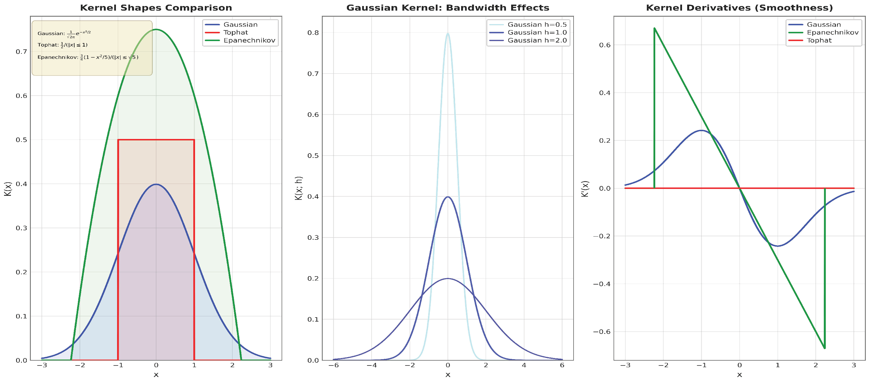
This section introduces the proposed continuous-variable Bayesian network learning framework. The framework uses KDE to estimate mutual information, conditional mutual information, and conditional entropy, and integrates these quantities into the two stages of MMHC. Figure 1 illustrates several commonly used kernel functions and their bandwidth effects, which helps explain the smoothing behavior underlying KDE-based estimation. To improve the computational feasibility of repeated density estimation, an FFT-based implementation is further adopted. Within this framework, KDE-based information measures are used in place of the discrete-data-oriented dependence evaluation and scoring components in the original MMHC procedure.

3.1. Radial Symmetric Kernel Estimation

KDE has been widely used as a nonparametric statistical method and has obviated the need for prior assumptions regarding the data distribution [49]. Instead, it infers the underlying density directly from observed samples, enabling adaptation to diverse data types and distributional patterns. The kernel functions employed are radial symmetric. In this study, a Gaussian-kernel-based KDE approach is adopted to estimate mutual information, conditional mutual information, and conditional entropy. A radial symmetric kernel refers to a class of kernel functions whose values depend only on the distance between input points, independent of direction. Such kernels typically possess rotational isotropy, shift invariance, and directional independence. Gaussian kernel is a typical symmetric kernel, which is exploited in the FFT-based convolution reformulation so that kernel discretization and repeated density evaluation can be accelerated. To accelerate computation, symmetric kernels are combined with FFT techniques, thereby significantly reducing computational complexity and enhancing the speed of estimation. Let $\{Z_1,\dots ,Z_i,\dots ,Z_N\}$, with $Z_i\in {\mathbb{R}}^d$, denote a set of independent and identically distributed random variables drawn from an unknown multivariate probability density function F. The expression for the multivariate standard KDE was given as follows [50]:

$$f_{\mathbf{H}}\left(\mathbf{s}\right)={\displaystyle \frac{1}{N}}{\displaystyle \sum _{i=1}^N}{K}_{\mathbf{H}}(\mathbf{s}-Z_i)={\displaystyle \frac{1}{N}}{\displaystyle \sum _{i=1}^N}{\displaystyle \frac{1}{{\left|\mathbf{H}\right|}^{1/2}}}K\left({\mathbf{H}}^{-1/2}(\mathbf{s}-Z_i)\right)$$

(4)

where $f\left(\mathbf{s}\right)$ denotes the probability density function estimated by KDE, and $\left|\mathbf{H}\right|$ denotes the determinant of $\mathbf{H}$. This notation was adopted following [51]. Here, K denotes the kernel function, and N denotes the sample size. Although KDE admits several kernel choices, including the Gaussian [52], Tophat [53], and Epanechnikov kernels [54], the present framework uses the Gaussian kernel for density estimation. Figure 1 is retained only as a qualitative background illustration of kernel shape and bandwidth effects.

$$K\left(u\right)={\displaystyle \frac{1}{\sqrt{2\pi }}}{e}^{-{\displaystyle \frac{u^2}{2}}};$$

(5)

$$K\left(u\right)={\displaystyle \frac{1}{2}}(1-u^2)·{\mathbf{1}}_{\left\{\right|u|\le 1\}}$$

(6)

The density estimation formula based on a multidimensional Gaussian kernel is given below.

$$f_{\mathbf{H}}\left(\mathbf{s}\right)={\displaystyle \frac{1}{N}}{\displaystyle \sum _{i=1}^N}{\displaystyle \frac{1}{{\left(2\pi \right)}^{d/2}{\left|\mathbf{H}\right|}^{1/2}}}exp\left(-{\displaystyle \frac{1}{2}}{(\mathbf{s}-Z_i)}^T{\mathbf{H}}^{-1}(\mathbf{s}-Z_i)\right)$$

(7)

If the bandwidth matrix is diagonal, the above expression can be simplified as follows [55]:

$$f_{\mathbf{H}}\left(\mathbf{s}\right)={\displaystyle \frac{1}{N}}{\displaystyle \sum _{i=1}^N}{\displaystyle \prod _{j=1}^d}{\displaystyle \frac{1}{{\left(2\pi \right)}^{1/2}{h}_j}}exp\left(-{\displaystyle \frac{1}{2}}{({\displaystyle \frac{s_j-Z_{ij}}{h_j}})}^2\right)$$

(8)

Relevant dependency measures can then be derived from the estimated density distribution. A symmetric kernel function is a fundamental prerequisite for accelerating KDE using the fast Fourier transform. Such symmetry ensures transformation invariance, allowing KDE as a standard convolution operation. Moreover, symmetry guarantees that the Fourier transform of the kernel is both real and even, which significantly simplifies computations in the frequency domain. After grid discretization, symmetry also reduces computational redundancy by half when evaluating kernel values. Equally important, symmetric kernels are fully compatible with real-valued convolution implemented via the FFT, eliminating the additional computational overhead associated with complex arithmetic. In contrast, using an asymmetric kernel makes direct FFT-based acceleration infeasible or requires complex frequency-domain manipulations, thereby negating any potential gains in computational efficiency.

3.2. FFT-Based Multivariate Kernel Density Estimation

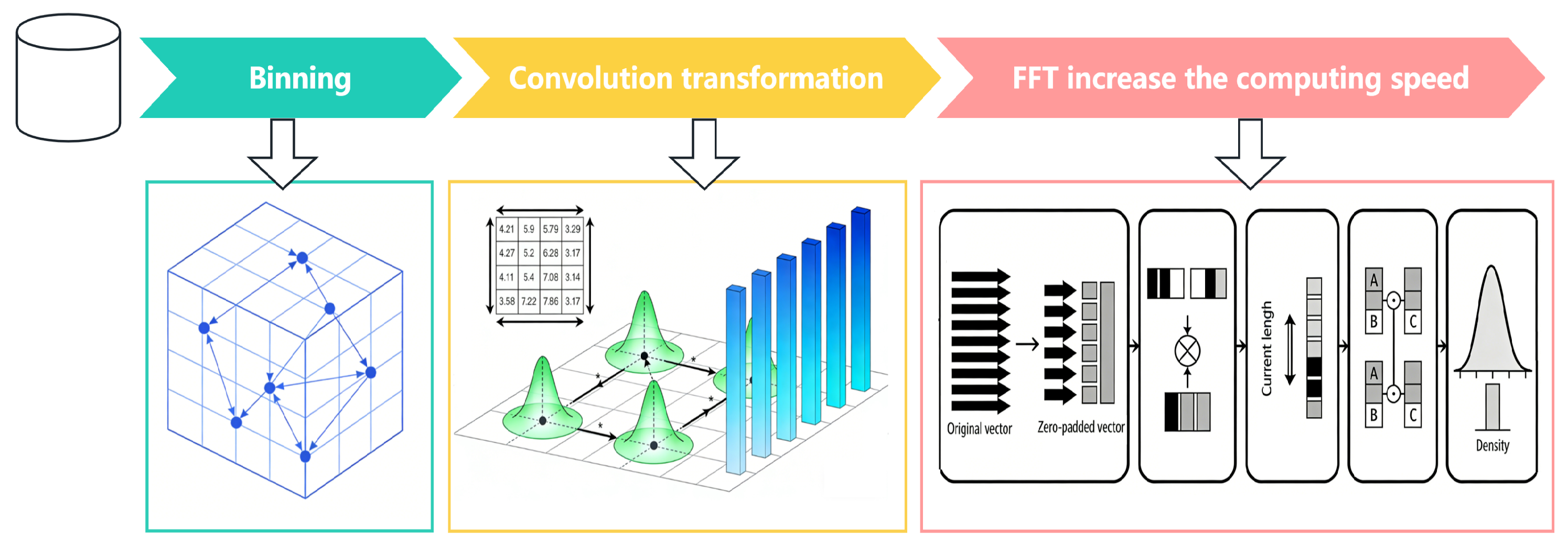
This study addresses a critical limitation in FFT-based multivariate KDE algorithms, which have traditionally operated accurately only with diagonal bandwidth matrices. Figure 2 shows the stages of KDE acceleration. First, each data point is assigned to its nearest grid point through data binning, yielding a grid-count vector that records the number of samples in each grid cell. Then, following the bandwidth matrix and grid spacing described in [56], the kernel function was discretized over the grid points by means of convolution-based kernel transformation. This step generates a kernel-weight vector and rewrites the density estimation formula as a discrete convolution of the grid counts and the kernel weights. Zero-padding is then applied to make the sequence length a highly composite number for FFT-accelerated convolution, after which the density estimate is computed via the FFT. Finally, the results are extracted from the inverse FFT and normalized to obtain the smoothed final estimate. We present a comprehensive solution that extends FFT-based KDE to support unconstrained bandwidth matrices, thereby enabling full utilization of orientation information in multivariate density estimation while maintaining computational efficiency. The complete FFT-based density estimation procedure is summarized in Algorithm 1. KDE represents one of the most fundamental statistical tools for nonparametric density estimation and has found extensive applications across a wide range of scientific domains, including pattern recognition, data visualization, and statistical inference. The multivariate KDE after binning is rewritten through a discrete convolution formulation, and the transformed kernel function is defined as follows [57,58].

Figure 2. Kernel density estimation by using FFT. The asterisk (*) denotes the convolution operation in the FFT-based KDE procedure.

Figure 2. Kernel density estimation by using FFT. The asterisk (*) denotes the convolution operation in the FFT-based KDE procedure.

$$K_{\mathbf{H}}\left(u\right)={\left|\mathbf{H}\right|}^{-\mathbf{1}/\mathbf{2}}\mathbf{K}\left({\mathbf{H}}^{-\mathbf{1}/\mathbf{2}}\mathbf{u}\right)$$

(9)

where $\mathbf{H}$ denotes the symmetric positive definite $d\times d$ bandwidth matrix, N denotes the sample size, ${\mathbf{Z}}_i$ denotes a d-variate observation, and K typically denotes the multivariate normal kernel function, following [57]. The computational complexity of direct KDE evaluation has been shown to scale as $O\left(mN\right)$ for m evaluation points and N data points [58], becoming prohibitively expensive for large datasets and higher dimensions. The FFT has provided an elegant computational framework for accelerating KDE through the convolution theorem [59]. According to this theorem, convolution in the spatial domain corresponds to pointwise multiplication in the frequency domain. The seminal work established a three-step FFT-based algorithm for multivariate KDE. The linear binning step is achieved by discretizing the input data onto equally spaced grid points ${\mathit{g}}_j$ with corresponding grid counts ${\mathit{c}}_l$. A weight is assigned to each grid point ${\mathit{g}}_l$. The above equation is then rewritten as Equation (10), which represents the sum of contributions from the original data points allocated to that specific grid location during the binning process. The number of grid points in dimension i, denoted by $M_i$, defines the resolution of the discretization in that direction. The equally spaced grid is fundamental to improving efficiency by converting density estimation into convolution operations and enabling FFT-based acceleration. Its grid spacing and range are adjustable to balance accuracy and computational cost and therefore require optimization according to the bandwidth parameters. In addition, through extended padding techniques, this grid framework supports convolution calculations with non-diagonal bandwidth matrices, thereby enabling the treatment of more complex density estimation problems.

$$\tilde{\mathit{f}}({\mathit{g}}_{\mathit{j}},\mathit{H},\mathit{M})={\displaystyle \frac{1}{N}}{\displaystyle \sum _{l_1=1}^{M_1}}\dots {\displaystyle \sum _{l_i=1}^{M_i}}\dots {\displaystyle \sum _{l_d=1}^{M_d}}{K}_{\mathit{H}}\left({\mathit{g}}_{\mathit{j}}-{\mathit{g}}_{\mathit{l}}\right){\mathit{c}}_{\mathit{l}}$$

(10)

where ${\mathit{g}}_{\mathit{l}}=(g{1}_{l1},\dots ,g{d}_{ld})$. In other words, the binning operation replaces the original dataset with a tuple structure $({\mathit{g}}_{\mathit{l}}$, ${\mathit{c}}_{\mathit{l}})$ of size $(M_1\times \dots \times M_d)$. The grid counts are higher at grid points located in regions with greater data concentration. The second step is performed through a convolution formulation. It reformulates the binned approximation as a discrete convolution. It should be emphasized that this binning step is introduced as a numerical approximation for fast convolution, rather than as a statistical discretization step for replacing continuous-variable structure learning. Unlike discretization-based BN learning, the proposed framework still performs smoothed density estimation and computes information-theoretic quantities in the continuous domain. The approximation error introduced by binning is therefore a numerical error controlled by grid resolution and truncation settings, rather than an information-loss mechanism of the type criticized in the Introduction.

$${\tilde{f}}_j={\displaystyle \sum _{l_1=-(M_1-1)}^{M_1-1}}\dots {\displaystyle \sum _{l_i=-(M_i-1)}^{M_i-1}}\dots {\displaystyle \sum _{l_d=-(M_d-1)}^{M_d-1}}{\mathit{c}}_{j-l}{\mathit{k}}_l,{\mathit{k}}_l={\displaystyle \frac{1}{N}}{K}_{\mathit{H}}({\delta }_1{l}_1,\dots ,{\delta }_i{l}_i,\dots ,{\delta }_d{l}_d)$$

(11)

In the FFT computation, the convolution theorem is employed to compute the density estimate through FFT operations. Here, j and l are multi-dimensional indices. ${\delta }_i$ denotes the grid spacing in the i-th dimension. $k_l$ is the kernel weight vector, which represents the discrete sampling of the kernel function on the grid.

$$\mathit{C}=F\left(\mathit{c}\right),\mathit{K}=F\left(\mathit{k}\right),\mathit{S}=\mathit{C}\mathit{K},\mathit{s}=F^{-1}\left(\mathit{S}\right)$$

(12)

The computational complexity is reduced from $O(M_1^2\dots M_d^2)$ to $O(M_{1}log{M}_1\dots M_{d}log{M}_d)$, representing substantial computational savings for practical applications. The conventional FFT-based algorithm suffers from a critical limitation, as it operates accurately only with constrained bandwidth matrices $H\in D$. When H is not diagonal, the off-diagonal entries encode cross-variable correlations and kernel orientation. In the proposed implementation, these correlations are retained through the transformed kernel representation induced by $H^{-1/2}$, so that the discretized kernel weights and subsequent FFT-based convolution preserve both scale and orientation information rather than forcing an axis-aligned approximation.

The fundamental issue lies in the wrap-around ordering procedure used in traditional FFT convolution. For diagonal bandwidth matrices, the kernel exhibits symmetry properties that align with the coordinate axes, ensuring that entries like $k_{-1,2}$ and $k_{1,2}$ remain equivalent. Empirical validation has demonstrated that the corrected algorithm produces results identical to direct computation while maintaining the computational efficiency of FFT-based approaches. The methodology extends beyond direct density estimation to facilitate fast computation of functionals crucial for optimal bandwidth selection, thereby contributing to the broader ecosystem of nonparametric statistical methods. This work represents a substantial advancement in the practical implementation of multivariate KDE, bridging the gap between statistical theory and computational feasibility.

Algorithm 1 FFT-based KDE algorithm

Input: Dataset D; bandwidth matrix $\mathbf{H}$; Grid size $(M_1,M_2,\dots ,M_d)$; truncation $\tau$; Output: FFT-KDE value $\tilde{\mathit{f}}$ and ${\mathit{g}}_{\mathit{l}}$  1: Discretize all data points $X_i$ in D onto a regular grid with equal grid size $(M_1\times M_2\times \dots \times M_d)$  2: Compute the grid points ${\mathit{g}}_{\mathit{l}}=(g_{1l_1},\dots ,g_{d{l}_d})$ and grid counts ${\mathit{c}}_{\mathit{l}}$  3: Compute the number of data points falling into each grid cell  4: Calculate the mesh size vector $\delta$ = (${\delta }_1$, …, ${\delta }_i$, …, ${\delta }_d$)  5: Compute the eigenvalues $\lambda$ of bandwidth matrix $\mathbf{H}$  6: for $i\in 1$ to d do  7:     Compute the convolution range using $L_i=min\left(M_i-1,\mathrm{floor}\left({\displaystyle \frac{\tau \sqrt{{\lambda }_i}}{{\delta }_i}}\right)\right)$  8: end for  9: Compute the kernel weights ${\mathbf{k}}_{\mathrm{new}}$ with $k_{\mathbf{l}}={\displaystyle \frac{1}{N}}{K}_{\mathbf{H}}({\delta }_1{l}_1,\dots ,{\delta }_d{l}_d)$ using Equation (9) 10: Extend the nearest power of two value $P_i$ using $L_i$. 11: Compute the ${\mathbf{c}}_{\mathrm{new}}$ by placing it in the central region. 12: Zero-pad ${\mathbf{k}}_{\mathrm{new}}$ and ${\mathbf{c}}_{\mathrm{new}}$ to large size $(P_1\times \cdots P_i\cdots \times P_d)$ 13: Compute FFT value $\mathbf{K}=\mathcal{F}\left({\mathbf{k}}_{\mathrm{new}}\right)$, $\mathbf{C}=\mathcal{F}\left({\mathbf{c}}_{\mathrm{new}}\right)$ 14: Compute element-wise multiplication and inverse transform $\mathbf{S}=\mathbf{K}\odot \mathbf{C},\mathbf{s}={\mathcal{F}}^{-1}\left(\mathbf{S}\right)$ 15: Compute the density values over the effective area and normalize ${\tilde{f}}_{\mathbf{j}}={\displaystyle \frac{s_{\mathbf{j}}}{P_1{P}_2\dots P_d}}$ 16: Output $\tilde{\mathit{f}}$ and ${\mathit{g}}_{\mathit{l}}$

3.3. Conditional Entropy Calculation Based on FFTKDE

To improve computational efficiency, the input data are discretized using the binning Equation (10). Each dimension i is divided into $M_i$ intervals, resulting in grid points ${\mathit{g}}_{\mathit{l}}=(g_{1l_1},g_{2l_2},\dots ,g_{d{l}_d}),l_i=1,\dots ,M_i$ where $\mathit{l}=(l_1,\dots ,l_d)$ is a multi-dimensional index. Let ${\mathbf{c}}_{\mathbf{l}}$ be the number of sample points falling into the bin represented by grid point ${\mathit{g}}_{\mathit{l}}$. The binned kernel density estimate is given in the above equation. For simplicity, the two-dimensional case $d=2$, involving random variables X and Y, is considered below. Let the grid points for X be $g_a^{\left(1\right)},a=1,\dots ,M_X$, and for Y be $g_b^{\left(2\right)},b=1,\dots ,M_Y$. Assuming uniform partitioning, $\Delta x$ and $\Delta y$ denote the grid widths. The estimate of the joint density ${\tilde{f}}_{XY}$ at grid point $(g_a^{\left(1\right)},g_b^{\left(2\right)})$ is given in the following equation.

$${\tilde{f}}_{XY}(g_a^{\left(1\right)},g_b^{\left(2\right)})={\displaystyle \frac{1}{N}}{\displaystyle \sum _{p=1}^{M_X}}{\displaystyle \sum _{q=1}^{M_Y}}{K}_{\mathbf{H}}\left((g_a^{\left(1\right)}-g_p^{\left(1\right)},g_b^{\left(2\right)}-g_q^{\left(2\right)})\right)c_{pq}$$

(13)

where $c_{pq}$ is the sample count at grid point $(g_p^{\left(1\right)},g_q^{\left(2\right)})$.

The estimate of the marginal density ${\tilde{f}}_X$ at point $g_a^{\left(1\right)}$ is obtained by integrating over Y:

$${\tilde{f}}_X\left(g_a^{\left(1\right)}\right)={\displaystyle \sum _{b=1}^{M_Y}}{\tilde{f}}_{XY}(g_a^{\left(1\right)},g_b^{\left(2\right)})\Delta y$$

(14)

Similarly, the estimate of the marginal density ${\tilde{f}}_Y$ at point $g_b^{\left(2\right)}$ is given by the following equation.

$${\tilde{f}}_Y\left(g_b^{\left(2\right)}\right)={\displaystyle \sum _{a=1}^{M_X}}{\tilde{f}}_{XY}(g_a^{\left(1\right)},g_b^{\left(2\right)})\Delta x$$

(15)

Mutual information for continuous random variables is defined as follows:

$$I(X;Y)=\int \int f_{XY}(x,y)log{\displaystyle \frac{f_{XY}(x,y)}{f_X\left(x\right)f_Y\left(y\right)}}dxdy$$

(16)

Discretizing this formula and substituting the above estimators for the true densities yields

$${\widehat{I}}_{\mathrm{KDE}}={\displaystyle \sum _{a=1}^{M_X}}{\displaystyle \sum _{b=1}^{M_Y}}\left[{\tilde{f}}_{XY}(g_a^{\left(1\right)},g_b^{\left(2\right)})\Delta x\Delta y\right]log{\displaystyle \frac{{\tilde{f}}_{XY}(g_a^{\left(1\right)},g_b^{\left(2\right)})\Delta x\Delta y}{\left({\tilde{f}}_X\left(g_a^{\left(1\right)}\right)\Delta x\right)\left({\tilde{f}}_Y\left(g_b^{\left(2\right)}\right)\Delta y\right)}}$$

(17)

Note that $\Delta x$ and $\Delta y$ cancel out between numerator and denominator, giving the final form.

$${\widehat{I}}_{\mathrm{KDE}}={\displaystyle \sum _{a=1}^{M_X}}{\displaystyle \sum _{b=1}^{M_Y}}\left({\tilde{f}}_{XY}(g_a^{\left(1\right)},g_b^{\left(2\right)})\Delta x\Delta y\right)log{\displaystyle \frac{{\tilde{f}}_{XY}(g_a^{\left(1\right)},g_b^{\left(2\right)})}{{\tilde{f}}_X\left(g_a^{\left(1\right)}\right){\tilde{f}}_Y\left(g_b^{\left(2\right)}\right)}}$$

(18)

3.4. MMHC-FFTKDE Algorithm Based on FFTKDE

The proposed framework for continuous-variable BN learning consists of two closely connected components, namely MMPC-FFTKDE and MMHC-FFTKDE. In the skeleton discovery stage, MMPC-FFTKDE uses FFTKDE to estimate mutual information and conditional mutual information, rather than relying on statistical tests designed for discrete data, thereby providing a dependency evaluation scheme that is more suitable for continuous variables. The corresponding skeleton discovery procedure is summarized in Algorithm 2. Based on the learned skeleton, the overall MMHC-FFTKDE framework then performs the subsequent search stage, in which candidate structures are evaluated using an FFTKDE-based conditional-entropy criterion instead of the conventional BIC score. In this way, FFTKDE is embedded into both local dependency screening and global structure refinement, allowing the proposed method to establish a unified learning procedure for continuous data and to improve the practical efficiency of BN structure learning. The overall MMHC-FFTKDE framework is presented in Algorithm 3.

Algorithm 2 MMPC-FFTKDE algorithm

Input: Target variable $v_t$; Dataset D; Variable set $V=\{v_1,\dots ,v_n\}$; Threshold value $\beta$ Output: $CPC\left(v_t\right)$  1: Initialize $CPC\left(v_t\right)=\varnothing$  2: repeat  3:     Calculate $AssocF={max}_{v\in V}{min}_{CS\subseteq CPC\left(v_t\right)}\widehat{I}(v,v_t\mid CS)$  4:     Calculate $v_F=arg{max}_{v\in V}{min}_{CS\subseteq CPC\left(v_t\right)}\widehat{I}(v,v_t\mid CS)$  5:     if $AssocF=0$ then  6:         $CPC\left(v_t\right)=CPC\left(v_t\right)$  7:     else  8:         $CPC\left(v_t\right)=CPC\left(v_t\right)\cup \left\{v_F\right\}$  9:     end if 10: until $CPC\left(v_t\right)$ does not change 11: for  $v\in CPC\left(v_t\right)$  do 12:     if $\exists CS\subseteq CPC\left(v_t\right)\setminus \left\{v\right\}$ such that $\widehat{I}(v,v_t\mid CS)<\beta$ then 13:         $CPC\left(v_t\right)=CPC\left(v_t\right)\setminus \left\{v\right\}$ 14:     else 15:         $CPC\left(v_t\right)=CPC\left(v_t\right)$ 16:     end if 17: end for

Algorithm 3 MMHC-FFTKDE algorithm

Input: Dataset D; Variable set $V=\{v_1,\dots ,v_n\}$; Threshold value $\beta$ Output: DAG $G=(V,E)$  1: Constraint phase:  2: for $v_t\in V$  do  3:     $CPC\left(v_t\right)=\mathrm{MMPC}\text{-}\mathrm{FFTKDE}(v_t,D,V,\beta )$ using Algorithm 2  4:     for $v\in CPC\left(v_t\right)$ do  5:         if $v_t\in \mathrm{MMPC}\text{-}\mathrm{FFTKDE}(v,D,V,\beta )$ then  6:            $CPC\left(v_t\right)=CPC\left(v_t\right)$  7:         else  8:            $CPC\left(v_t\right)=CPC\left(v_t\right)-\left\{v\right\}$  9:         end if 10:     end for 11: end for 12: Search phase: 13: Initialize network structure G 14: repeat 15:     $currentScore=Evaluate\left(G\right)$ using Equations (20)–(22) 16:     $bestScore=currentScore$ 17:     $bestGraph=G$ 18:     $G_0=GenerateCandidates\left(G\right)$ 19:     for $G_i\in G_0$ do 20:         $candidateScore=Evaluate\left(G_i\right)$ using Equations (20)–(22) 21:         if $candidateScore>bestScore$ then 22:            $bestGraph=G_i$ 23:            $bestScore=candidateScore$ 24:         end if 25:     end for 26:     if $bestScore>currentScore$ then 27:         $G=bestGraph$ 28:     end if 29: until $bestScore\le currentScore$

The MMPC-FFTKDE algorithm is a method for identifying candidate parent–child sets of target variables in BN structure learning. The algorithm operates in two main phases: forward selection and backward elimination. In the forward selection phase, it employs a max–min strategy to progressively build the candidate set. The max–min selection principle was described in [60]. Specifically, for each variable not currently in the candidate set, the algorithm evaluates its association with the target variable by calculating the minimum conditional mutual information across all possible subsets of the current candidate set, using FFTKDE-based density estimation to evaluate these information-theoretic measures. It then selects the variable that maximizes this minimum association value and adds it to the candidate set, because this variable exhibits the strongest conditional dependence with the target variable, even under the most challenging conditioning circumstances. This iterative process continues until no additional variables can be added, meaning that the candidate set has reached a stable configuration in which all remaining variables outside the set show negligible conditional dependence. Subsequently, in the backward elimination phase, the algorithm performs a thorough verification of each variable within the candidate set. For every candidate variable, it examines whether there exists any conditional subset among the remaining candidates that causes its conditional mutual information with the target variable to fall below a predefined significance threshold. If such a conditional independence relationship is detected, indicating that the variable’s apparent association with the target can be explained by other variables, it is removed from the candidate set. This elimination step ensures that only those variables that maintain a direct, non-redundant conditional relationship with the target variable are retained. Through this two-phase approach, which combines forward selection based on max–min association with backward elimination based on conditional independence testing, the algorithm ultimately produces a stable, compact candidate parent–child set that captures the most relevant direct dependencies for the target variable. Procedure 15 in Algorithm 3 uses add-edge, delete-edge, and reverse-edge to modify the current network structure G locally, thereby obtaining a series of candidate network structures $G_0$. The algorithm only applies the add-edge operator $v_t\to v$ if $v\in CPC\left(v_t\right)$. For a node $v_i$ with parent set ${\Pi }_i$, the local score used in the search stage is defined by the following equation.

$$h_{score}(v_i\mid {\Pi }_i)=-H(v_i\mid {\Pi }_i)=H(\mid {\Pi }_i\mid )-H(v_i\cup \mid {\Pi }_i\mid )$$

(19)

where $\mid {\Pi }_i\mid$ indicates the parent variables in set ${\Pi }_i$. Equations (20)–(22) are special cases of this general definition for empty, one-parent, and two-parent sets, respectively. This method does not introduce an explicit complexity penalty. Under limited samples, the conditional entropy using kernel density estimation has a variance buffering effect on the introduction of irrelevant variables, and adding irrelevant variables does not systematically improve the score.

$$h_{score}(v_1\mid \Pi )=-H\left(v_1\right)$$

(20)

$$h_{score}(v_1\mid {\Pi }_1)=H\left(v_2\right)-H(v_1,v_2)$$

(21)

$$h_{score}(v_1\mid {\Pi }_1^{\prime })=H(v_2,v_3)-H(v_1,v_2,v_3)$$

(22)

The overall computational cost of MMHC-FFTKDE is determined by both the constraint phase and the search phase. In the constraint phase, the main cost comes from repeated FFTKDE-based evaluations of mutual information and conditional mutual information for candidate parent–child discovery. In the search phase, the cost is dominated by repeated conditional-entropy evaluations of candidate structures during hill-climbing. Therefore, the total complexity can be viewed as the sum of the numbers of dependency-evaluation calls and structure-scoring calls, each multiplied by the cost of a single FFTKDE-based density evaluation. Under fixed grid resolution, the FFT-based implementation reduces the practical cost of each repeated density-estimation step, although the total runtime still depends on the number of variables, the search space explored, the conditioning-set size, and the selected implementation parameters.The present comparison therefore focuses on empirical runtime behavior rather than on a unified asymptotic complexity comparison across heterogeneous baseline implementations, since the compared methods differ substantially in search strategy, dependency evaluation mechanism, and optimization procedure.

3.5. Implementation Details

In the current implementation, the bandwidth used in KDE and FFTKDE is selected by the same rule-of-thumb strategy to ensure comparability between the two estimators. This choice provides a simple and reproducible setting for the present study, although it is not intended to claim optimality across all data distributions.

The grid resolution and truncation range affect the numerical behavior of FFTKDE. A finer grid and a larger truncation range generally reduce approximation error, but they also increase memory usage and computation time. More importantly, because the total number of grid points scales as $M_1\dots M_d$, the regular-grid FFT implementation is mainly suitable for low-to-moderate dimensional settings rather than very high-dimensional problems. In the present study, the main density-estimation experiments are conducted for $d=10$, 20, and 40, and additional higher-dimensional results for $d=60$ and 80 are further included to examine the practical behavior of the method as dimensionality increases. When the dimensionality becomes substantially larger, grid growth can become a practical bottleneck unless further techniques such as sparse grids, adaptive binning, or dimensionality reduction are introduced. Therefore, the current implementation should be viewed as a computationally efficient solution for low-to-moderate dimensional continuous-variable structure learning, with limited empirical extension to higher-dimensional settings, rather than as a fully scalable high-dimensional KDE framework.

The main computational burden in the proposed framework comes from repeated density estimation during conditional-independence evaluation and structure scoring. Direct KDE evaluates densities in the spatial domain, whereas FFTKDE reformulates the computation through binning and convolution on regular grids and then performs acceleration in the frequency domain. As a result, the practical gain depends on the sample size, variable dimension, grid size, and the number of repeated estimation calls within the learning process.

4. Experiment Results

4.1. Compare FFTKDE with KDE in Curve Fitting Performance

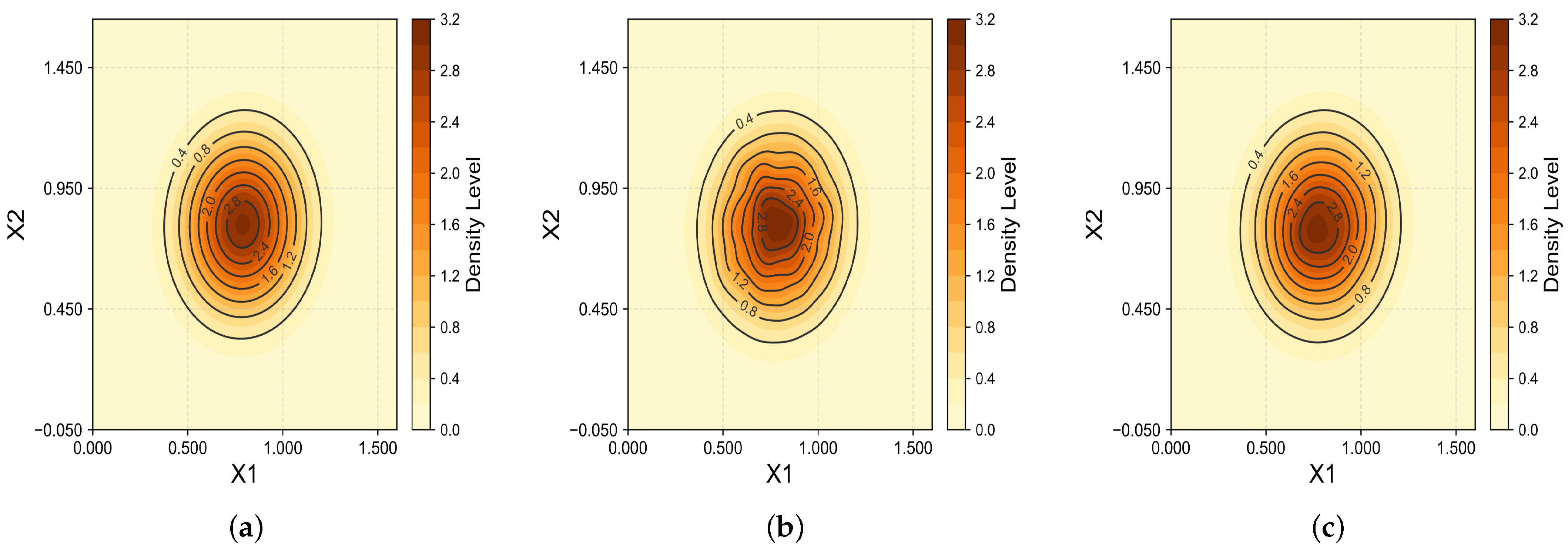
To verify the density-estimation performance of FFTKDE, a controlled two-dimensional Gaussian example is used. The mean vector is set to $\left[\begin{array}{c}0.8\\ 0.8\end{array}\right]$, and the covariance matrix is specified as $\left[\begin{array}{cc}0.05& 0\\ 0& 0.05\end{array}\right]$. A total of 7000 samples are generated. Both KDE and FFTKDE adopt the same classical rule-of-thumb bandwidth selection. The truncation parameter $\tau$ determines the balance between approximation fidelity and computational cost. A larger value preserves more kernel information and generally improves fitting accuracy, but it also increases the number of grid points involved in convolution. A smaller value reduces the computational burden, yet may introduce truncation errors near the estimation boundaries. In this experiment, the bandwidth parameters for both FFTKDE and KDE are obtained by using rule of thumb, truncation $\tau$ is 3.0, and the grid parameters $M_1$ and $M_2$ are 100. The corresponding fitting results are shown in Figure 3.

The figure presents the contour distributions of the reference probability density function (PDF), KDE, and FFTKDE. The contour lines represent different density levels, while the filled colors indicate the corresponding density magnitude. The color bar on the right provides the mapping between color intensity and density value. It can be observed that the FFTKDE estimate preserves the main geometric characteristics of the target density, including the location of the density peak and the overall contour concentration pattern. The difference between FFTKDE and conventional KDE is very small under the current sample size, indicating that the FFT-based reformulation maintains density-estimation fidelity while providing a more efficient computational scheme.

To further examine estimation fidelity under different distributions and dimensional settings, multidimensional synthetic samples were generated and evaluated by mean squared error (MSE) with respect to the corresponding reference densities. In this setting, a smaller MSE indicates a closer approximation to the target density and better fitting accuracy. The parameter configurations used for data generation are summarized in

Table 1. Parameter settings for different multi-dimensional distribution.

Gaussian	T-Distribution	Cauchy	Laplace
$\mu$ = [${\mu }_1$, …, ${\mu }_d$]; ${\mu }_1$ = ${\mu }_d$ = 0; $\delta$ = $\left[\begin{array}{ccc}{\delta }_1& \dots & 0\\ ⋮& \ddots & ⋮\\ 0& \dots & {\delta }_d\end{array}\right]$; ${\delta }_1$ = ${\delta }_d$ = 1;	$loc=[l_1,\dots ,l_d]$; $l_1=l_d=0$; $scale=\left[\begin{array}{ccc}{s}_1& \dots & 0\\ ⋮& \ddots & ⋮\\ 0& \dots & s_d\end{array}\right]$; $df=5$; $s_1=s_d=1$	$loc=[l_1,\dots ,l_d]$; $l_1=l_d=0$; $scale=\left[\begin{array}{ccc}{s}_1& \dots & 0\\ ⋮& \ddots & ⋮\\ 0& \dots & s_d\end{array}\right]$; $df=1$; $s_1=s_d=1$	$loc=[l_1,\dots ,l_d]$; $l_1=l_d=0$; $\Sigma$ = $\left[\begin{array}{ccc}{b}_1& \dots & 0\\ ⋮& \ddots & ⋮\\ 0& \dots & b_d\end{array}\right]$; $b_1$ = $b_d=2$

, and the estimation results obtained by KDE and FFTKDE are reported in

Table 2. Comparison of estimation accuracy and runtime across different data distributions.

Distribution	Method	d = 10	Time	d = 20	Time	d = 40	Time	d = 60	Time	d = 80	Time
Gaussian	KDE	$3.12\times {10}^{-7}$	22.5	$3.21\times {10}^{-6}$	22.6	$3.03\times {10}^{-4}$	22.2	$5.11\times {10}^{-4}$	23.0	$7.66\times {10}^{-4}$	23.8
	FFTKDE	$3.28\times {10}^{-7}$	9.7	$3.24\times {10}^{-6}$	10.9	$3.05\times {10}^{-4}$	9.8	$5.18\times {10}^{-4}$	10.4	$7.74\times {10}^{-4}$	11.2
T-distribution	KDE	$1.27\times {10}^{-6}$	22.7	$5.35\times {10}^{-6}$	22.8	$1.57\times {10}^{-4}$	22.4	$2.61\times {10}^{-4}$	23.2	$3.95\times {10}^{-4}$	24.0
	FFTKDE	$1.28\times {10}^{-6}$	9.9	$5.55\times {10}^{-6}$	11.1	$1.58\times {10}^{-4}$	10.0	$2.67\times {10}^{-4}$	10.6	$4.02\times {10}^{-4}$	11.4
Cauchy	KDE	$4.56\times {10}^{-6}$	23.0	$1.00\times {10}^{-6}$	23.1	$4.23\times {10}^{-4}$	22.7	$6.12\times {10}^{-4}$	23.5	$9.08\times {10}^{-4}$	24.4
	FFTKDE	$4.54\times {10}^{-6}$	10.2	$1.02\times {10}^{-6}$	11.4	$4.24\times {10}^{-4}$	10.3	$6.19\times {10}^{-4}$	10.9	$9.17\times {10}^{-4}$	11.8
Laplace	KDE	$1.19\times {10}^{-7}$	22.6	$6.15\times {10}^{-6}$	22.7	$2.41\times {10}^{-4}$	22.3	$3.48\times {10}^{-4}$	23.1	$5.19\times {10}^{-4}$	23.9
	FFTKDE	$1.13\times {10}^{-7}$	9.8	$6.12\times {10}^{-6}$	11.0	$2.43\times {10}^{-4}$	9.9	$3.56\times {10}^{-4}$	10.5	$5.27\times {10}^{-4}$	11.3

Parameters: sample size = 18,000, error is represented by MSE, runtime is in seconds.

. The experiments cover five settings for different dimensions, namely 10, 20, 40, 60, and 80. In the controlled density-estimation experiment, the bandwidth parameter for each dimension is still rule of thumb. The default FFT grid resolution is set to $M_i=100$ for each dimension, and the truncation parameter is fixed at $\tau =3.0$. As shown in Table 2, both KDE and FFTKDE become more computationally demanding as dimensionality increases, and the MSE also tends to rise accordingly. Nevertheless, the difference in fitting accuracy between the two methods remains small across all tested distributions and dimensional settings, indicating that FFTKDE maintains estimation fidelity comparable to that of conventional KDE while preserving a clear runtime advantage.

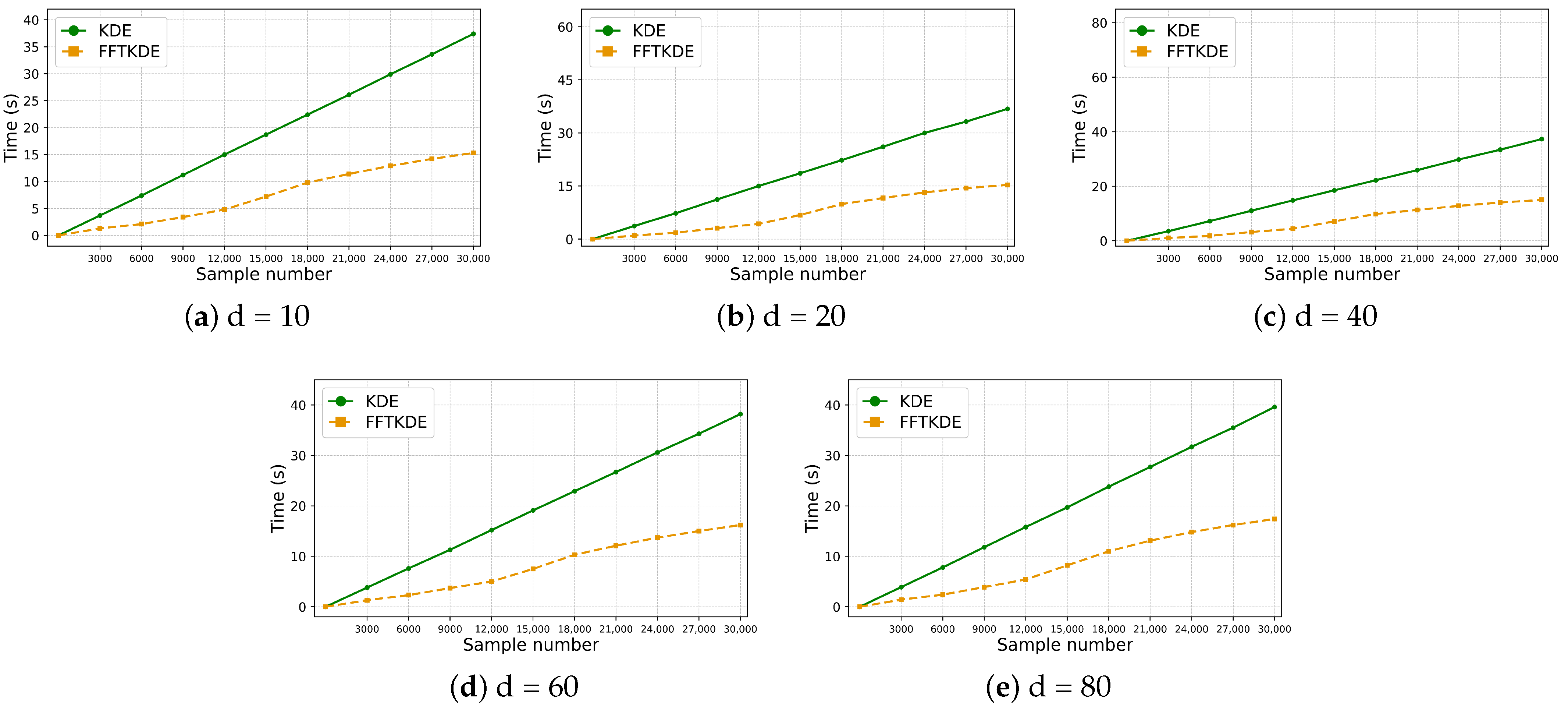
To further assess computational efficiency with respect to sample size, simulated samples were generated from a standard T-distribution with $df=30$. Experiments were conducted in 10, 20, 40, 60, and 80 dimensions, with sample sizes ranging from 3000 to 30,000. The corresponding runtime results are shown in Figure 4. It can be observed that the FFT-based implementation consistently requires less computation time than direct KDE. As the sample size increases, the runtime of both methods rises steadily, but the increase is much more moderate for FFTKDE, resulting in an increasingly evident runtime gap between the two methods. These results indicate that the computational advantage of FFT-based acceleration becomes more apparent when repeated density estimation is carried out on larger datasets. In addition, although higher dimensionality leads to a general increase in runtime for both methods, FFTKDE still preserves a clear efficiency advantage over conventional KDE in all tested cases.

4.2. Sensitivity Analysis of Bandwidth and Grid Settings

We use the parameters in

Table 3. Sensitivity analysis under different bandwidth, grid-size, and truncation settings using T-distribution.

Bandwidth	Grid Size	Truncation Parameter	MSE	Runtime (s)
0.5	100	3.0	0.084	12.6
0.7	100	3.0	0.061	12.7
1.0	100	3.0	0.079	12.6
0.7	200	3.0	0.062	18.2
0.7	200	4.0	0.061	18.1
0.7	200	5.0	0.059	18.3
0.7	100	3.0	0.061	12.7
0.7	200	3.0	0.062	18.2
0.7	300	3.0	0.058	19.9

to examine the sensitivity of FFTKDE to key implementation parameters, which are bandwidth, grid size, and truncation setting. The results show that parameter selection has a direct influence on both estimation fidelity and computational efficiency. By using the same grid size and truncation, bandwidth mainly affects the smoothness of density estimation and therefore changes the resulting MSE. Grid size and truncation setting determine the numerical resolution and convolution range used in the FFT-based implementation, and thus influence both approximation quality and runtime. A finer grid generally improves estimation accuracy, but this gain is accompanied by increased computational cost. Similarly, different bandwidth values produce different estimation behaviors, indicating that excessively small or excessively large bandwidths are both suboptimal for the tested setting. These results indicate that the chosen parameter configuration strikes an effective balance between estimation error and computational runtime. Accordingly, this sensitivity analysis not only elucidates the numerical behavior of FFTKDE across various settings but also furnishes empirical support for the parameter choices employed in the subsequent structure-learning experiments.

4.3. Comparative Analysis of BN Structure Learning Algorithms

4.3.1. Datasets and Evaluation Metrics

In this study, benchmark BNs such as CHILD, INSURANCE, and ALARM [61] are used for algorithm testing and accuracy evaluation. As these benchmark networks are originally defined for discrete variables, the continuous datasets required for the experiments are generated by linear structural equations based on the structural relationships of the given reference networks [62].

To reduce the limitations of relying only on a simple linear synthetic setting, additional data-generating mechanisms are introduced in this subsection. These settings are constructed to vary both the structural functional form and the noise distribution, allowing the proposed framework to be examined under more challenging continuous-variable scenarios.

The synthetic settings reported in

Table 4. Synthetic data-generating settings used in the extended experiments.

Structural Relation Equation	Format	Relation	Noise Type	Description
${\displaystyle v_i=w^{T}Pa\left(v_i\right)+{\epsilon }_i,{\epsilon }_i\sim \mathcal{N}(0,1)}$	${\kappa }_1$	Linear	Gaussian	baseline setting
${\displaystyle v_i=\sum _j{a}_{j}sin\left(P{a}_j\right)+{\epsilon }_i,{\epsilon }_i\sim \mathcal{N}(0,1)}$	${\kappa }_2$	Nonlinear	Gaussian	nonlinear relation
${\displaystyle v_i=\sum _j{a}_{j}sin\left(P{a}_j\right)+{\epsilon }_i,{\epsilon }_i\sim \mathrm{Laplace}(0,1)}$	${\kappa }_3$	Nonlinear	Non-Gaussian	nonlinear with nonGaussian noise

include three representative continuous-data cases, namely a linear Gaussian baseline setting, a nonlinear Gaussian setting, and a nonlinear non-Gaussian setting. In this way, the benchmark comparison is extended beyond a single linear Gaussian scenario, allowing the behavior of the proposed framework to be evaluated under progressively more complex dependency structures and distributional conditions.

For the synthetic benchmark experiments, continuous datasets were generated according to the structural relations of the reference networks under the settings reported in Table 4. Specifically, ${\kappa }_1$ corresponds to a linear Gaussian setting, in which each variable is generated as a linear combination of its parent variables with an additive Gaussian noise term. ${\kappa }_2$ introduces nonlinear structural relations by replacing the linear parent effect with a sinusoidal form while retaining Gaussian noise. ${\kappa }_3$ further combines the nonlinear structural relation with non-Gaussian Laplace noise. In all cases, the corresponding coefficients were generated randomly so that the resulting datasets reflect different functional and distributional characteristics under the same benchmark topology. All generated samples were directly used for structure-recovery evaluation against the known benchmark graphs, following a common protocol in benchmark-based structure-learning studies. This setting is suitable for comparing graph-recovery behavior under controlled conditions, although it does not evaluate generalization on unseen data. We therefore regard this as a limitation of the current experimental design. Precision (P), recall (R), and F1-score ($F1$) were used as basic indicators of edge-recovery performance by comparing the learned structures with the corresponding benchmark networks. To provide a more complete evaluation, Structural Hamming distance ($SHD$) and runtime are also reported in the extended experiments. These metrics together reflect edge recovery, structural discrepancy, and computational cost. The present evaluation is primarily focused on structure-recovery quality rather than downstream predictive likelihood or intervention-based predictive performance. The Structural Intervention Distance (SID) is not included in the current study, because the present experiments are designed primarily for benchmark-based graph-recovery comparison under repeated synthetic settings.

$$P={\displaystyle \frac{TP}{TP+FP}}R={\displaystyle \frac{TP}{TP+FN}}F1={\displaystyle \frac{2PR}{P+R}}$$

(23)

where $TP$ is the number of correctly recognized edges, $FP$ is the number of incorrectly recognized edges, and $FN$ is the number of missed true edges. A reversed edge is treated as an error in edge-recovery evaluation, and SHD is computed in the standard directed-graph sense.

4.3.2. Performance Comparison

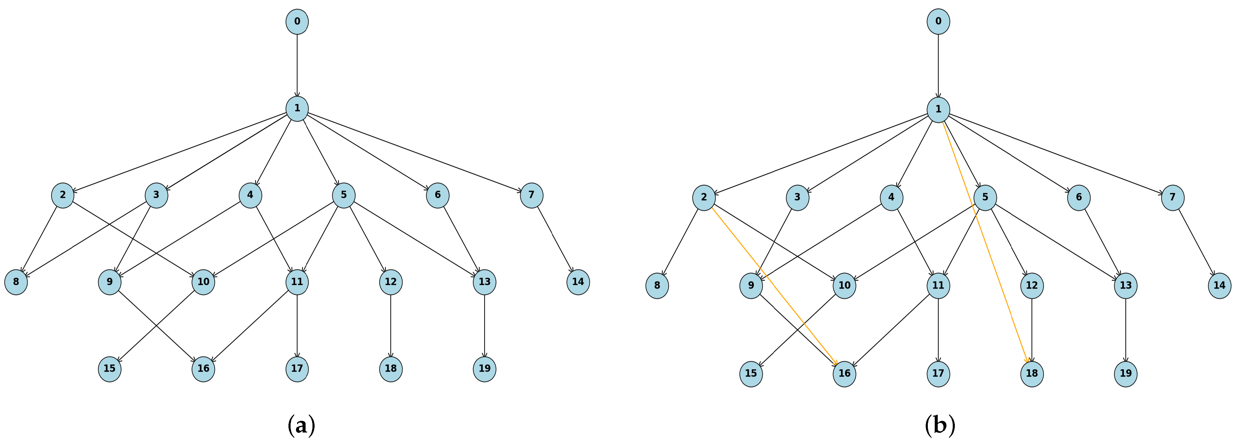
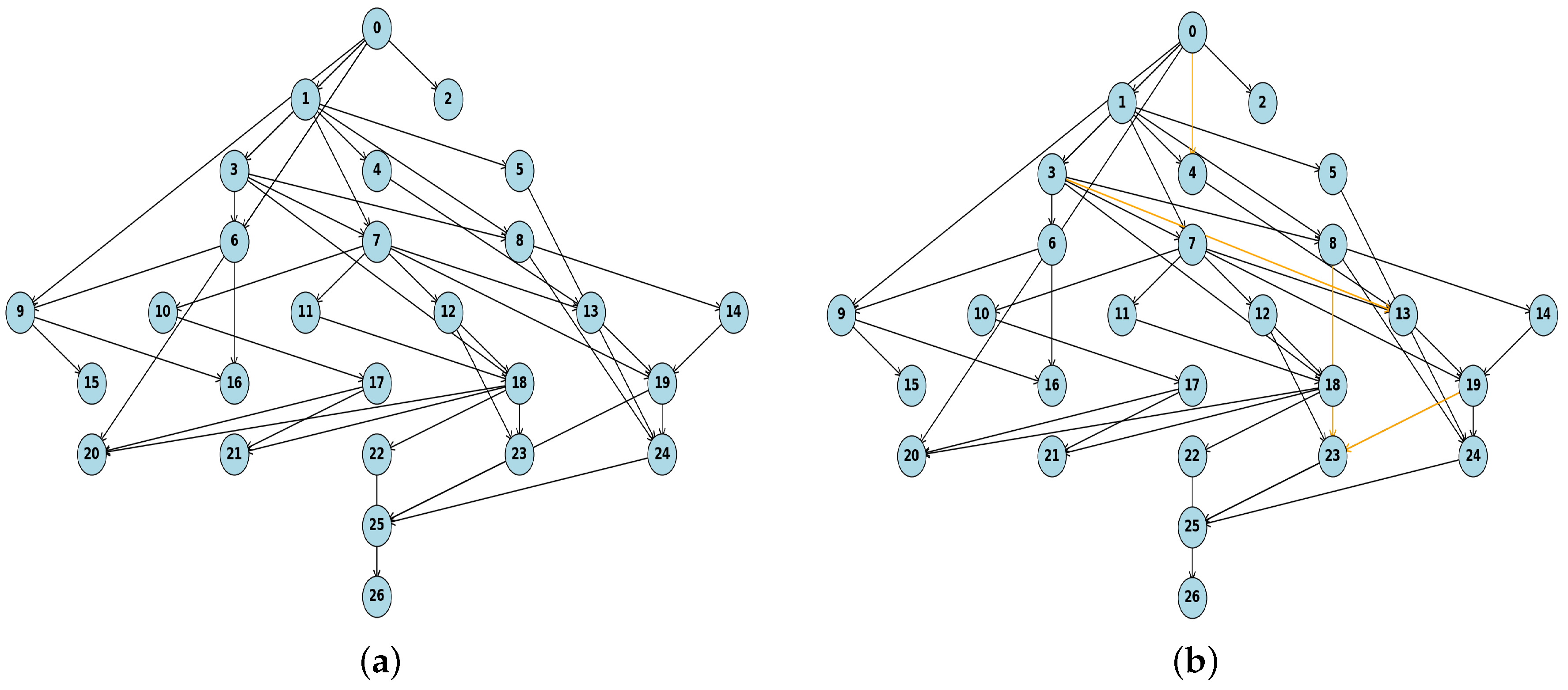
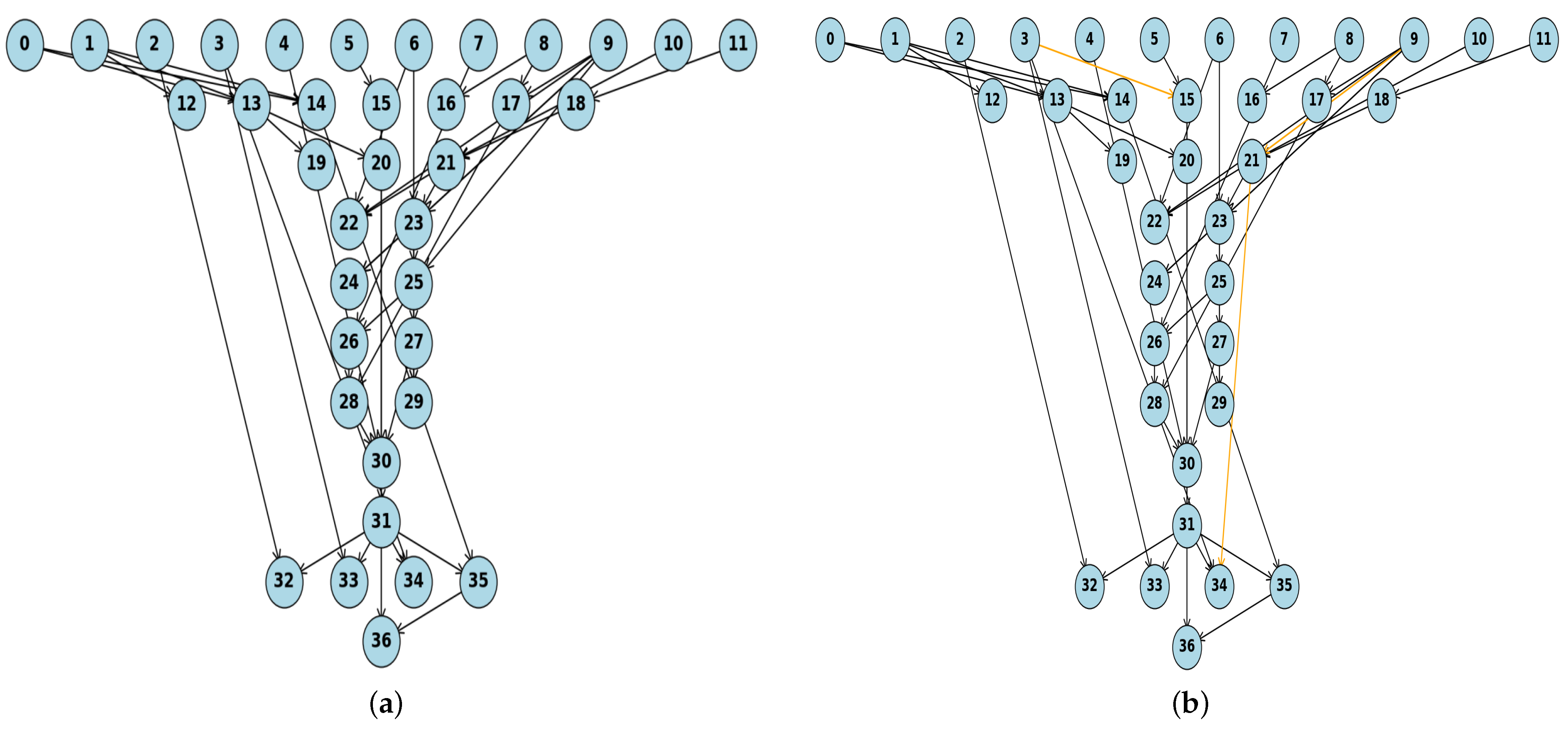
To evaluate the effectiveness of the algorithm proposed in this paper for BN structure learning, three well-known network structures were selected for the experiments. The CHILD network consists of 20 nodes and 25 edges. The INSURANCE network contains 27 nodes and 52 edges. The ALARM network contains 37 nodes and 46 edges. For the visualized benchmark results in this subsection, the continuous data were generated under the F1 setting. The reference structures of these three networks are shown in Figure 5a, Figure 6a and Figure 7a, and the network structures obtained using the MMHC-FFTKDE algorithm are shown in Figure 5b, Figure 6b and Figure 7b. In these figures, consistent edges are highlighted in black, and incorrectly detected edges are marked in orange.

The significance threshold $\beta$ used in MMPC-FFTKDE is fixed at 0.01 commonly, which is adopted as a conservative default significance level and it is kept unchanged across benchmark settings to avoid dataset-specific tuning. To compare the learning performance of representative structure-learning methods, IAMB-KDE, HITON-PC-KDE, L1MB, PCB, NOTEARS, and MMHC-FFTKDE are evaluated on the benchmark networks under the three synthetic data-generating settings considered in this study. In the IAMB-KDE algorithm, the Gaussian kernel is typically used as the kernel function, the bandwidth is set to the default adaptive rules, the significance level is set to 0.1 to determine the strictness of conditional independence tests, and the algorithm terminates when the candidate Markov blanket no longer changes. The common parameter settings for HITON-PC-KDE are a significance level of 0.05, KDE bandwidth using adaptive rules, maximum conditioning set size of 2, and that the algorithm stops when the candidate parent–child set no longer changes. The uniform strategy, which is a equal-width binning strategy, is applied for each bin. We set the number of bins with 10 for each dimension. The key parameter for L1MB is the L1 regularization coefficient $\lambda$ set to 0.01 or selected by cross-validation, and the core parameter for PCB is the significance level $\alpha$ set to 0.05, and the key parameters for NOTEARS are the L1 regularization coefficient set to 0.8 and the edge threshold set to 0.3, where all three methods learn causal structures by controlling sparsity.

These baselines are chosen because they provide representative constraint-based, hybrid, regularization-based, and optimization-based reference points for continuous-variable Bayesian network structure learning and remain directly comparable to the proposed MMHC-style framework. In the experiments, equal-width binning is adopted where required in order to balance statistical reliability and information retention.

The corresponding performance results under the ${\kappa }_1$, ${\kappa }_2$, and ${\kappa }_3$ settings are reported in

Table 5. Comparison of structure-learning performance on benchmark networks using the ${\kappa }_1$ formula.

Network	Sample Size	Method	Precision	Recall	F1	SHD	Runtime
ALARM	5500	IAMB-KDE	$0.849\pm 0.08$	$0.883\pm 0.05$	$0.861\pm 0.03$	$11.200\pm 1.38$	$94.500\pm 4.00$
	5500	HITON-PC-KDE	$0.875\pm 0.06$	$0.893\pm 0.04$	$0.882\pm 0.02$	$9.700\pm 1.24$	$100.600\pm 4.30$
	5500	L1MB	$0.872\pm 0.07$	$0.883\pm 0.05$	$0.874\pm 0.02$	$10.200\pm 1.29$	$68.300\pm 3.00$
	5500	PCB	$0.869\pm 0.08$	$0.878\pm 0.05$	$0.870\pm 0.02$	$10.600\pm 1.33$	$77.200\pm 3.30$
	5500	NOTEARS	$0.886\pm 0.06$	$0.891\pm 0.04$	$0.886\pm 0.02$	$9.300\pm 1.18$	$109.400\pm 4.80$
	5500	MMHC-FFTKDE	$0.913\pm 0.04$	$0.959\pm 0.03$	$0.935\pm 0.02$	$6.800\pm 0.92$	$53.900\pm 2.40$
CHILD	5500	IAMB-KDE	$0.905\pm 0.07$	$0.900\pm 0.06$	$0.900\pm 0.04$	$4.500\pm 0.97$	$79.600\pm 3.40$
	5500	HITON-PC-KDE	$0.916\pm 0.03$	$0.900\pm 0.06$	$0.907\pm 0.03$	$4.100\pm 0.88$	$86.100\pm 3.70$
	5500	L1MB	$0.911\pm 0.06$	$0.884\pm 0.07$	$0.896\pm 0.05$	$4.900\pm 1.02$	$60.200\pm 2.70$
	5500	PCB	$0.897\pm 0.04$	$0.884\pm 0.05$	$0.889\pm 0.03$	$5.300\pm 1.10$	$69.400\pm 3.00$
	5500	NOTEARS	$0.911\pm 0.04$	$0.892\pm 0.06$	$0.901\pm 0.04$	$4.400\pm 0.95$	$97.500\pm 4.20$
	5500	MMHC-FFTKDE	$0.928\pm 0.04$	$0.940\pm 0.04$	$0.933\pm 0.02$	$3.200\pm 0.63$	$47.800\pm 2.10$
INSURANCE	5500	IAMB-KDE	$0.871\pm 0.08$	$0.827\pm 0.05$	$0.845\pm 0.02$	$10.800\pm 1.21$	$86.400\pm 3.80$
	5500	HITON-PC-KDE	$0.882\pm 0.06$	$0.850\pm 0.04$	$0.863\pm 0.01$	$9.600\pm 1.08$	$91.500\pm 4.00$
	5500	L1MB	$0.895\pm 0.07$	$0.844\pm 0.05$	$0.865\pm 0.02$	$9.300\pm 1.02$	$63.600\pm 2.80$
	5500	PCB	$0.885\pm 0.08$	$0.837\pm 0.06$	$0.856\pm 0.01$	$10.100\pm 1.14$	$72.800\pm 3.20$
	5500	NOTEARS	$0.897\pm 0.07$	$0.850\pm 0.05$	$0.869\pm 0.02$	$9.000\pm 1.00$	$102.300\pm 4.50$
	5500	MMHC-FFTKDE	$0.939\pm 0.04$	$0.931\pm 0.05$	$0.933\pm 0.02$	$6.500\pm 0.86$	$50.300\pm 2.20$

,

Table 6. Comparison of structure-learning performance on benchmark networks using ${\kappa }_2$ formula.

Network	Sample Size	Method	Precision	Recall	F1	SHD	Runtime
ALARM	5500	IAMB-KDE	$0.838\pm 0.09$	$0.868\pm 0.05$	$0.850\pm 0.03$	$12.000\pm 1.45$	$101.8\pm 4.4$
	5500	HITON-PC-KDE	$0.863\pm 0.07$	$0.881\pm 0.05$	$0.871\pm 0.03$	$10.500\pm 1.30$	$108.7\pm 4.7$
	5500	L1MB	$0.859\pm 0.07$	$0.870\pm 0.05$	$0.863\pm 0.03$	$11.000\pm 1.34$	$73.1\pm 3.2$
	5500	PCB	$0.857\pm 0.08$	$0.866\pm 0.05$	$0.861\pm 0.03$	$11.300\pm 1.38$	$82.6\pm 3.5$
	5500	NOTEARS	$0.876\pm 0.07$	$0.880\pm 0.04$	$0.878\pm 0.03$	$10.100\pm 1.24$	$117.9\pm 5.0$
	5500	MMHC-FFTKDE	$0.905\pm 0.05$	$0.948\pm 0.03$	$0.925\pm 0.02$	$7.400\pm 0.98$	$57.6\pm 2.6$
CHILD	5500	IAMB-KDE	$0.894\pm 0.07$	$0.888\pm 0.06$	$0.889\pm 0.05$	$5.000\pm 1.05$	$85.4\pm 3.7$
	5500	HITON-PC-KDE	$0.906\pm 0.04$	$0.888\pm 0.06$	$0.895\pm 0.04$	$4.700\pm 0.96$	$92.5\pm 4.0$
	5500	L1MB	$0.900\pm 0.06$	$0.872\pm 0.07$	$0.884\pm 0.05$	$5.400\pm 1.10$	$64.7\pm 2.9$
	5500	PCB	$0.885\pm 0.05$	$0.871\pm 0.06$	$0.876\pm 0.04$	$5.800\pm 1.16$	$74.3\pm 3.2$
	5500	NOTEARS	$0.900\pm 0.05$	$0.881\pm 0.06$	$0.889\pm 0.04$	$5.100\pm 1.04$	$104.8\pm 4.5$
	5500	MMHC-FFTKDE	$0.920\pm 0.05$	$0.928\pm 0.04$	$0.923\pm 0.03$	$3.800\pm 0.72$	$51.2\pm 2.3$
INSURANCE	5500	IAMB-KDE	$0.860\pm 0.08$	$0.815\pm 0.05$	$0.833\pm 0.03$	$11.500\pm 1.28$	$92.7\pm 4.0$
	5500	HITON-PC-KDE	$0.871\pm 0.07$	$0.838\pm 0.05$	$0.851\pm 0.03$	$10.300\pm 1.15$	$98.4\pm 4.3$
	5500	L1MB	$0.883\pm 0.08$	$0.832\pm 0.06$	$0.853\pm 0.03$	$10.000\pm 1.10$	$68.1\pm 3.0$
	5500	PCB	$0.874\pm 0.08$	$0.824\pm 0.06$	$0.844\pm 0.03$	$10.900\pm 1.22$	$78.2\pm 3.4$
	5500	NOTEARS	$0.885\pm 0.07$	$0.838\pm 0.05$	$0.857\pm 0.03$	$9.800\pm 1.08$	$109.6\pm 4.8$
	5500	MMHC-FFTKDE	$0.930\pm 0.05$	$0.919\pm 0.05$	$0.924\pm 0.02$	$7.200\pm 0.94$	$54.1\pm 2.4$

, and

Table 7. Comparison of structure-learning performance on benchmark networks using ${\kappa }_3$ formula.

Network	Sample Size	Method	Precision	Recall	F1	SHD	Runtime
ALARM	5500	IAMB-KDE	$0.828\pm 0.09$	$0.854\pm 0.06$	$0.840\pm 0.04$	$12.800\pm 1.52$	$108.9\pm 4.7$
	5500	HITON-PC-KDE	$0.851\pm 0.08$	$0.867\pm 0.05$	$0.858\pm 0.03$	$11.300\pm 1.39$	$116.0\pm 5.0$
	5500	L1MB	$0.846\pm 0.08$	$0.856\pm 0.06$	$0.850\pm 0.03$	$11.800\pm 1.42$	$78.4\pm 3.4$
	5500	PCB	$0.844\pm 0.08$	$0.852\pm 0.06$	$0.847\pm 0.03$	$12.100\pm 1.46$	$88.3\pm 3.8$
	5500	NOTEARS	$0.864\pm 0.07$	$0.867\pm 0.05$	$0.865\pm 0.03$	$10.900\pm 1.33$	$125.7\pm 5.4$
	5500	MMHC-FFTKDE	$0.894\pm 0.05$	$0.936\pm 0.04$	$0.914\pm 0.02$	$8.200\pm 1.05$	$61.9\pm 2.7$
CHILD	5500	IAMB-KDE	$0.884\pm 0.08$	$0.875\pm 0.06$	$0.878\pm 0.05$	$5.600\pm 1.12$	$91.2\pm 4.0$
	5500	HITON-PC-KDE	$0.896\pm 0.05$	$0.875\pm 0.06$	$0.884\pm 0.04$	$5.200\pm 1.03$	$98.7\pm 4.3$
	5500	L1MB	$0.889\pm 0.07$	$0.859\pm 0.07$	$0.872\pm 0.05$	$5.900\pm 1.18$	$69.0\pm 3.1$
	5500	PCB	$0.875\pm 0.06$	$0.858\pm 0.06$	$0.865\pm 0.04$	$6.300\pm 1.23$	$79.1\pm 3.5$
	5500	NOTEARS	$0.889\pm 0.05$	$0.868\pm 0.06$	$0.877\pm 0.04$	$5.800\pm 1.15$	$111.8\pm 4.9$
	5500	MMHC-FFTKDE	$0.910\pm 0.05$	$0.917\pm 0.04$	$0.913\pm 0.03$	$4.300\pm 0.81$	$54.8\pm 2.5$
INSURANCE	5500	IAMB-KDE	$0.848\pm 0.09$	$0.801\pm 0.06$	$0.820\pm 0.03$	$12.300\pm 1.35$	$99.1\pm 4.3$
	5500	HITON-PC-KDE	$0.860\pm 0.07$	$0.824\pm 0.06$	$0.840\pm 0.03$	$11.100\pm 1.22$	$105.2\pm 4.6$
	5500	L1MB	$0.871\pm 0.08$	$0.818\pm 0.06$	$0.841\pm 0.03$	$10.800\pm 1.18$	$73.0\pm 3.2$
	5500	PCB	$0.862\pm 0.08$	$0.810\pm 0.06$	$0.832\pm 0.03$	$11.700\pm 1.30$	$83.7\pm 3.7$
	5500	NOTEARS	$0.873\pm 0.08$	$0.823\pm 0.06$	$0.844\pm 0.03$	$10.600\pm 1.16$	$117.0\pm 5.1$
	5500	MMHC-FFTKDE	$0.919\pm 0.05$	$0.906\pm 0.05$	$0.912\pm 0.03$	$7.900\pm 1.02$	$57.8\pm 2.6$

, respectively. Because the present study focuses on MMHC-style hybrid Bayesian network learning for continuous variables, the empirical comparison is restricted to methods that remain directly comparable in terms of dependency-evaluation mechanism or structure-learning objective. Broader comparisons with neural generative and additional kernel-based causal learners are left for future work.

Table 5, Table 6 and Table 7 provide a comparative summary of edge-recovery performance, structural discrepancy, and runtime across the evaluated methods under the ${\kappa }_1$, ${\kappa }_2$, and ${\kappa }_3$ data-generating settings, respectively. In addition to precision, recall, and F1-score, SHD and runtime are also reported, allowing the methods to be compared from both structural and computational perspectives. The relative performance of the evaluated methods varies across benchmark networks and data-generating settings. MMHC-FFTKDE shows competitive overall performance and, in several cases, achieves a favorable balance between structural accuracy and computational cost. These results therefore serve as the main basis for the comparative analysis in this subsection.

The bandwidth of each dimension is achieved by using adaptive rules, a grid size of 200 and truncation of 3.0. To assess whether the observed performance differences are statistically reliable, additional paired statistical tests are conducted over the repeated runs. Both a paired t-test and the Wilcoxon signed-rank test are used to compare MMHC-FFTKDE with the baseline methods under the same network and sample-size setting, and the p-values are given in

Table 8. Statistical significance analysis of repeated-run F1-score results.

Network	Sample Size	Baseline	t-Value	p-Value (t-Test)	p-Value (Wilcoxon)
ALARM	1500	IAMB-KDE	3.8358	0.003992	0.005859
	1500	HITON-PC-KDE	1.6151	0.140737	0.232422
	1500	L1MB	0.9837	0.350950	0.232422
	1500	PCB	1.2839	0.231230	0.232422
	1500	NOTEARS	1.3971	0.195858	0.193359
	5500	IAMB-KDE	10.3648	2.6535 $\times {10}^{-6}$	0.001953
	5500	HITON-PC-KDE	6.1956	1.5972 $\times {10}^{-4}$	0.001953
	5500	L1MB	7.7304	2.9078 $\times {10}^{-5}$	0.001953
	5500	PCB	7.2497	4.8179 $\times {10}^{-5}$	0.001953
	5500	NOTEARS	5.7019	2.9361 $\times {10}^{-4}$	0.001953
CHILD	1500	IAMB-KDE	3.4094	0.007757	0.013672
	1500	HITON-PC-KDE	2.5751	0.029935	0.048828
	1500	L1MB	3.2000	0.010832	0.005859
	1500	PCB	2.8509	0.019062	0.027344
	1500	NOTEARS	2.6538	0.026310	0.021484
	5500	IAMB-KDE	2.7908	0.021027	0.019531
	5500	HITON-PC-KDE	2.1336	0.061657	0.052734
	5500	L1MB	2.3955	0.040191	0.048828
	5500	PCB	4.0794	0.002761	0.005859
	5500	NOTEARS	2.0741	0.067906	0.083984
INSURANCE	1500	IAMB-KDE	5.1679	5.8885 $\times {10}^{-4}$	0.001953
	1500	HITON-PC-KDE	3.0398	0.014022	0.007812
	1500	L1MB	3.9922	0.003147	0.005859
	1500	PCB	3.3598	0.008392	0.013672
	1500	NOTEARS	3.5127	0.006591	0.003906
	5500	IAMB-KDE	12.1667	6.8453 $\times {10}^{-7}$	0.001953
	5500	HITON-PC-KDE	10.9216	1.7100 $\times {10}^{-6}$	0.001953
	5500	L1MB	11.1113	1.4788 $\times {10}^{-6}$	0.001953
	5500	PCB	23.1995	2.4440 $\times {10}^{-9}$	0.001953
	5500	NOTEARS	10.6563	2.1029 $\times {10}^{-6}$	0.001953

. These results provide further evidence regarding whether the observed performance improvements are statistically significant rather than due to random variation.

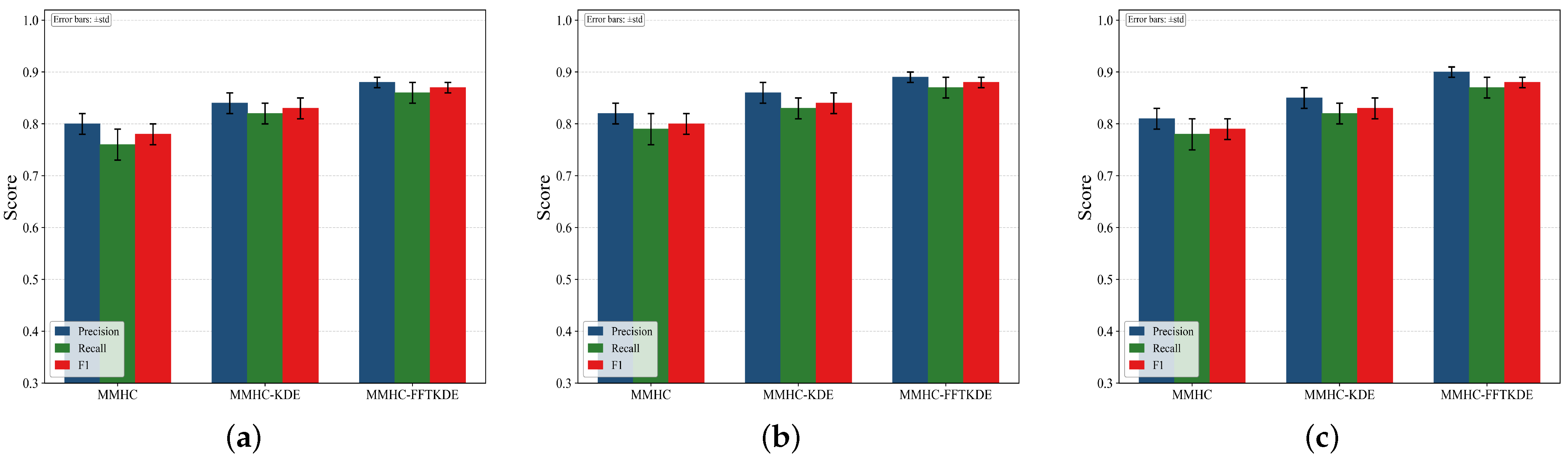
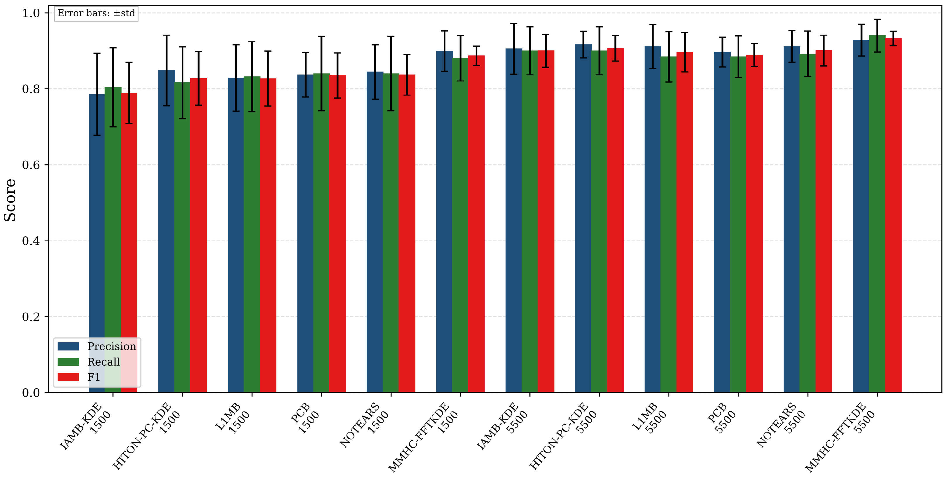
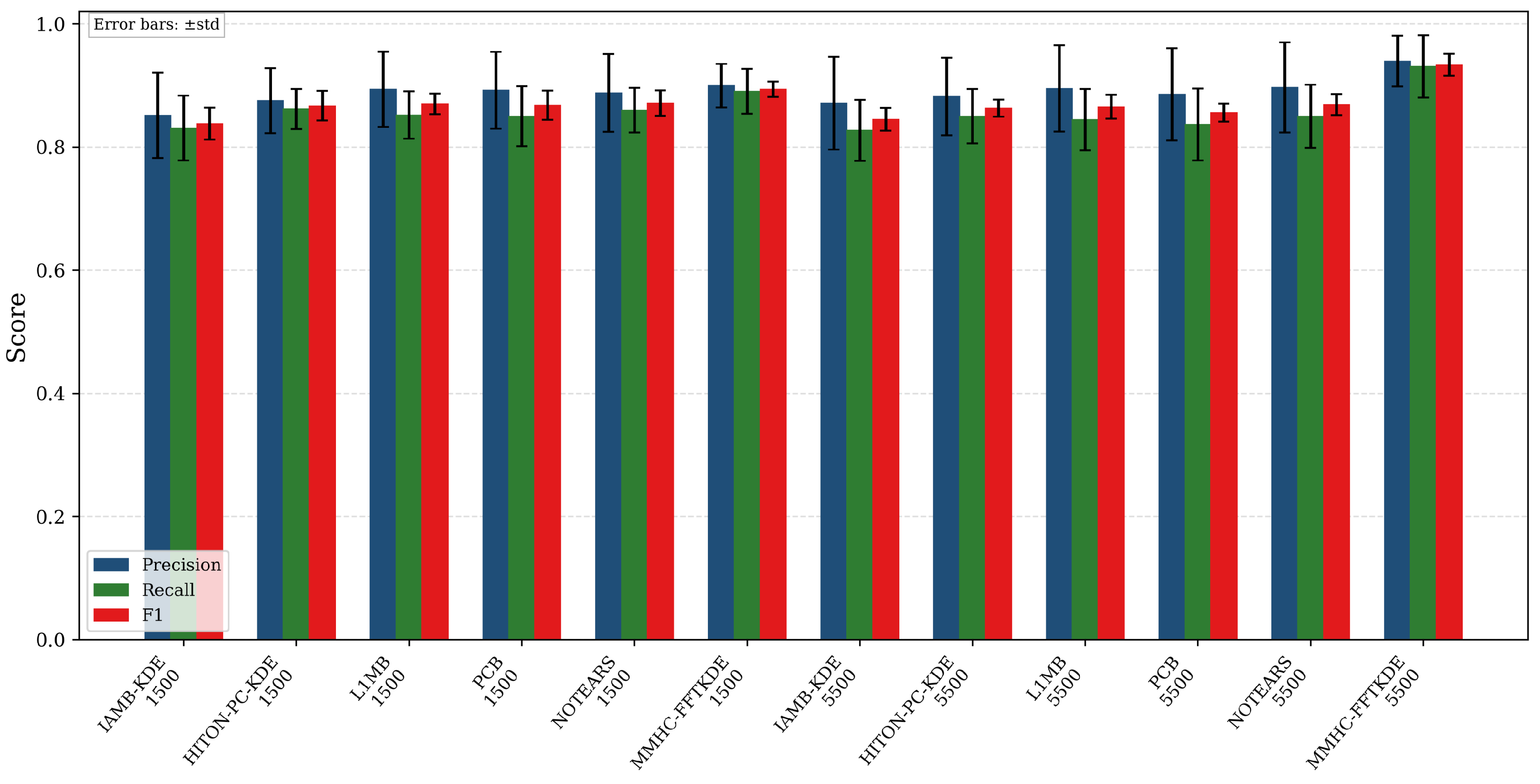
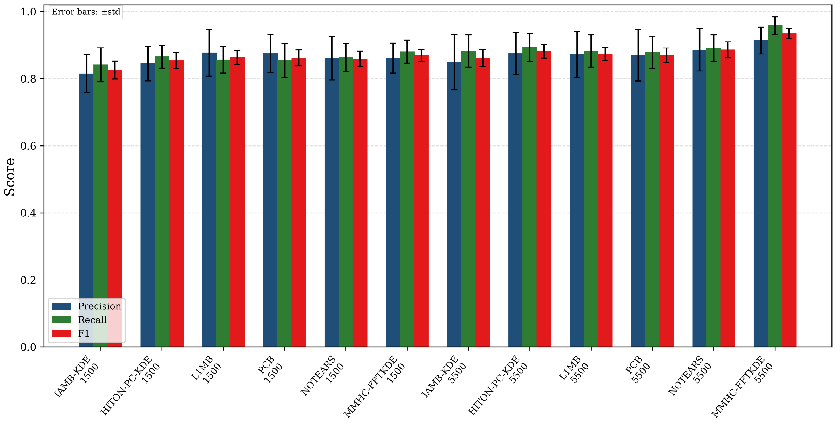
As shown in Figure 5, Figure 6 and Figure 7, the network structures inferred by MMHC-FFTKDE closely match the corresponding reference topologies and accurately recover parent–child dependencies. To further assess the effectiveness of the proposed method, this study compares the precision, recall, and F1-score of MMHC, MMHC-KDE, and MMHC-FFTKDE on the three benchmark networks [63]. It should be noted that the original MMHC algorithm requires the discretization of continuous data, whereas MMHC-KDE and MMHC-FFTKDE use KDE-based dependency estimation for continuous variables. For each network and sample-size setting, the experiment was repeated ten times, and the mean values and standard deviations of precision, recall, and F1-score were calculated. The resulting bar charts are presented with standard deviation error bars to show the variability of the repeated-run results more clearly. This three-method comparison is used to examine the effects of KDE-based dependency estimation and FFT-based acceleration within the MMHC framework. By contrast, the broader multi-method benchmark comparison under the F1, F2, and F3 settings is reported in Table 5, Table 6 and Table 7, whereas the paired statistical significance analysis reported in Table 8 includes results for sample sizes of 1500 and 5500.

As shown in Figure 8, the evaluated networks exhibit noticeable differences in edge-recovery performance. Figure 8 compares MMHC, MMHC-KDE, and MMHC-FFTKDE on the benchmark datasets using precision, recall, and F1-score with standard deviation error bars. This comparison illustrates the effects of KDE-based dependency estimation and FFT-based acceleration within the MMHC framework. For the INSURANCE network, the recall values of MMHC-KDE and MMHC-FFTKDE are both higher than that of the conventional MMHC algorithm. For the CHILD and ALARM networks, MMHC-KDE and MMHC-FFTKDE also achieve higher precision than MMHC. Overall, MMHC-KDE and MMHC-FFTKDE show comparable accuracy and generally perform better than the original MMHC under the tested setting. These observations suggest that avoiding direct discretization can be beneficial for continuous-variable structure learning, while the FFT-based implementation further improves the practical computational feasibility of KDE-based learning.

Figure 9, Figure 10 and Figure 11 further provide visual comparisons of precision, recall, and F1-score, with standard deviation error bars, across the evaluated methods under different sample-size settings. These figures show that, for most methods, larger sample sizes are associated with better edge-recovery performance. Across the tested benchmark networks, MMHC-FFTKDE remains competitive under both smaller- and larger-sample settings and achieves favorable accuracy in several cases. Together, these visual comparisons further support the comparative results reported in the corresponding tables.

4.3.3. Scalability with Conditioning-Set Size and Network Scale

To further examine the scalability of the proposed framework, additional experiments were conducted from two perspectives, namely conditioning-set size and network scale. The corresponding results are reported in

Table 9. Scalability of MMHC-KDE and MMHC-FFTKDE with conditioning-set size and network scale.

Factor	Setting	Method	F1	SHD	Runtime (s)
Conditioning-set size	$\mid CS\mid =1$	MMHC-KDE	0.88	5	27.9
		MMHC-FFTKDE	0.88	5	15.4
	$\mid CS\mid =2$	MMHC-KDE	0.86	6	41.2
		MMHC-FFTKDE	0.87	6	23.5
Network scale	20 nodes	MMHC-KDE	0.87	5	29.6
		MMHC-FFTKDE	0.88	5	17.3
	40 nodes	MMHC-KDE	0.83	9	56.8
		MMHC-FFTKDE	0.85	8	33.1
	60 nodes	MMHC-KDE	0.77	14	102.4
		MMHC-FFTKDE	0.80	12	61.7
	80 nodes	MMHC-KDE	0.71	19	168.9
		MMHC-FFTKDE	0.75	16	97.5

. In the first group of experiments, the size of the conditioning set was gradually increased in order to evaluate how repeated conditional-independence testing affects structural accuracy and runtime. In the second group, the number of network nodes was increased to assess the practical behavior of the method with larger graph structures.

As shown in Table 9, both MMHC-KDE and MMHC-FFTKDE experience performance degradation as the conditioning set becomes larger. F1-score decreases, SHD increases, and runtime grows substantially in both cases. Nevertheless, MMHC-FFTKDE remains consistently faster than MMHC-KDE across all tested settings, while preserving competitive structural accuracy. These results provide additional empirical evidence that the FFT-based implementation improves the computational feasibility of repeated KDE-based dependency estimation, although the overall difficulty of structure learning still increases with larger conditioning sets and larger network sizes.

4.3.4. Real-Data Case Study

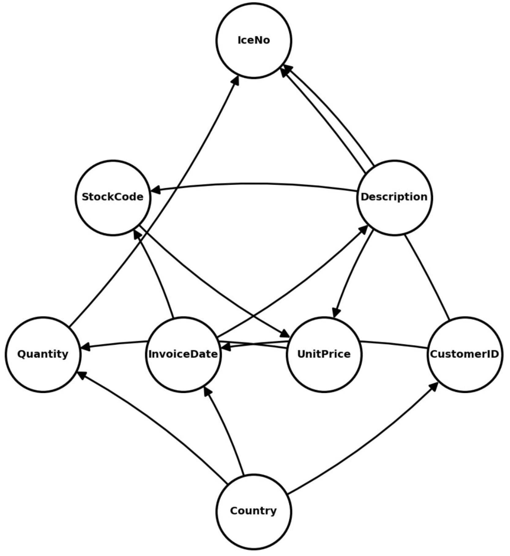
An open-source online retail dataset from the UCI Machine Learning Repository [64] is further used as a qualitative case study to illustrate the structure produced by the proposed method on real-world data. As no ground-truth causal graph is available for this dataset, the resulting network should not be interpreted as a validated causal structure. Instead, it is used to examine whether the learned dependencies are reasonably consistent with business semantics and variable co-occurrence patterns.

As shown in Figure 12, several variables related to customer identity, transaction time, product description, stock code, unit price, quantity, and invoice information are connected in an interpretable dependency pattern. For example, temporal and customer-related variables are linked to product-level variables, and product-level variables are further associated with price and quantity. These relationships provide a plausible descriptive structure for exploratory analysis. Therefore, this real-data example is intended to demonstrate the practical interpretability of the learned graph rather than to serve as a formal validation experiment.

5. Conclusions

This study developed a continuous-variable Bayesian network learning framework by integrating KDE-based information-theoretic estimation into the MMHC procedure and introducing an FFT-based implementation to reduce the cost of repeated density estimation. The experimental results indicate that, under the tested settings, the proposed framework maintains estimation fidelity comparable to that of conventional KDE while requiring less computation time, and it achieves competitive performance in benchmark-based structure-recovery experiments. Nevertheless, the present work should be regarded as a computationally enhanced hybrid framework for continuous-variable Bayesian network learning rather than as a complete theoretical solution to nonparametric causal structure learning. In particular, it does not provide a formal consistency proof for KDE-based conditional-independence testing, a complete theoretical characterization of the approximation effects introduced by the FFT-based implementation, or exact guarantees for structure recovery. Future work will therefore focus on these theoretical issues, together with broader evaluations under more challenging continuous-data settings.

References

1. Decampos, C.P.; Zeng, Z.; Ji, Q. Structure learning of Bayesian networks using constraints. In Proceedings of the 26th Annual International Conference on Machine Learning, Montreal, QC, Canada, 14–18 June 2009; pp. 113–120. Available online: https://dl.acm.org/doi/abs/10.1145/1553374.1553389 (accessed on 21 April 2026).
2. Zhang, J.; Shi, M.; Lang, X.; You, Q.; Jing, Y.; Huang, D.; Dai, H.; Kang, J. Dynamic risk evaluation of hydrogen station leakage based on fuzzy dynamic Bayesian network. Int. J. Hydrogen Energy 2024, 50, 1131–1145. [Google Scholar] [CrossRef] [Scilit]
3. Zhang, J.F.; Jin, M.; Wan, C.P.; Dong, Z.J.; Wu, X.H. A Bayesian network-based model for risk modeling and scenario deduction of collision accidents of inland intelligent ships. Reliab. Eng. Syst. Saf. 2024, 243, 109816. [Google Scholar] [CrossRef] [Scilit]
4. Ahsan, M.; Khan, A.; Khan, K.R.; Sinha, B.B.; Sharma, A. Advancements in medical diagnosis and treatment through machine learning: A review. Expert Syst. J. Knowl. Eng. 2024, 41, 13499. [Google Scholar] [CrossRef] [Scilit]
5. Fang, W.; Zhang, W.J.; Ma, L.; Wu, Y.L.; Yan, K.F.; Lu, H.Y.; Sun, J.; Wu, X.J.; Yuan, B. An efficient Bayesian network structure learning algorithm based on structural information. Swarm Evol. Comput. 2023, 76, 101224. [Google Scholar] [CrossRef] [Scilit]
6. Kitson, N.K.; Constantinou, A.C.; Guo, Z.G.; Liu, Y.; Chobtham, K. A survey of Bayesian network structure learning. Artif. Intell. Rev. 2023, 56, 8721–8814. [Google Scholar] [CrossRef] [Scilit]
7. Wang, X.C.; Ren, H.J.; Guo, X.X. A novel discrete firefly algorithm for Bayesian network structure learning. Knowl.-Based Syst. 2022, 242, 108426. [Google Scholar] [CrossRef] [Scilit]
8. Gao, W.; Zhi, M.; Ke, Y.; Wang, X.; Zhuo, Y.; Liu, A.; Yang, Y. Bayesian network structure learning based on HC-PSO algorithm. J. Intell. Fuzzy Syst. 2024, 46, 4347–4359. [Google Scholar] [CrossRef] [Scilit]
9. Lv, Y.L.; Miao, J.; Liang, J.; Liang, J.Y.; Chen, L.; Qian, Y.H. BIC-based node order learning for improving Bayesian network structure learning. Front. Comput. Sci. 2021, 15, 156337. [Google Scholar] [CrossRef] [Scilit]
10. Chen, E.Y.J.; Adnan, D.; Arthur, C. On Pruning with the MDL Score. Int. J. Approx. Reason. 2018, 92, 363–375. [Google Scholar] [CrossRef] [Scilit]
11. Bouchaala, L.; Masmoudi, A.; Gargouri, F.; Rebai, A. Improving algorithms for structure learning in Bayesian networks using a new implicit score. Expert Syst. Appl. 2010, 37, 5964–5974. [Google Scholar] [CrossRef] [Scilit]
12. Chickering, D.M. Optimal structure identification with greedy search. J. Mach. Learn. Res. 2002, 3, 507–554. [Google Scholar]
13. Li, H.H.; Cabeli, V.; Sella, N.; Isambert, H. Constraint-based causal structure learning with consistent separating sets. In Proceedings of the Advances in Neural Information Processing Systems, Vancouver, BC, Canada, 8–14 December 2019; pp. 14257–14266. Available online: https://proceedings.neurips.cc/paper/2019/hash/e6872f5bbe75073f8c7cfb93de7f6f3a-Abstract.html (accessed on 21 April 2026).
14. Martins, M.S.; Yafrani, M.E.; Delgado, M.; Lüders, R.; Santana, R.; Siqueira, H.V.; Akcay, H.G.; Ahiod, B. Analysis of Bayesian network learning techniques for a hybrid multi-objective Bayesian estimation of distribution algorithm: A case study on MNK landscape. J. Heuristics 2021, 27, 549–573. [Google Scholar] [CrossRef] [Scilit]
15. Jose, S.; Liu, S.; Louis, S.; Dascalu, S. Towards a hybrid approach for evolving Bayesian networks using genetic algorithms. In Proceedings of the IEEE International Conference on Tools with Artificial Intelligence, Portland, OR, USA, 4–6 November 2019; pp. 705–712. [Google Scholar] [CrossRef] [Scilit]
16. Wang, N.; Liu, H.R.; Zhang, L.Y.; Cai, Y.B.; Shi, Q.R. An efficient skeleton learning approach-based hybrid algorithm for identifying Bayesian network structure. Eng. Appl. Artif. Intell. 2024, 133, 108105. [Google Scholar] [CrossRef] [Scilit]
17. He, C.H.; Wang, P.; Tian, L.Y.; Di, R.H.; Wang, Z.D.; Yang, Y. A novel structure learning method of Bayesian networks based on the neighboring complete node ordering search. Neurocomputing 2024, 585, 127620. [Google Scholar] [CrossRef] [Scilit]
18. Mabrouk, A.; Gonzales, C.; Jabet-Chevalier, K.; Chojnaki, E. Multivariate cluster-based discretization for Bayesian network structure learning. In Proceedings of the 9th International Conference on Scalable Uncertainty Management, Québec City, QC, Canada, 16–18 September 2015; pp. 155–169. [Google Scholar] [CrossRef] [Scilit]
19. Dimitris, M. Distribution-Free Learning of Bayesian Network Structure in Continuous Domains. In Proceedings of the AAAI Conference on Artificial Intelligence, Pittsburgh, PA, USA, 9–13 July 2005; pp. 825–830. Available online: http://www.aaai.org/Library/AAAI/2005/aaai05-130.php (accessed on 21 April 2026).
20. Hao, Z.; Zhou, S.G.; Guan, J.H. Measuring conditional independence by independent residuals: Theoretical results and application in causal discovery. In Proceedings of the AAAI Conference on Artificial Intelligence, New Orleans, LA, USA, 2–7 February 2018; pp. 2029–2036. [Google Scholar] [CrossRef] [Scilit]
21. Bach, F.; Jordan, M. Learning Graphical Models with Mercer Kernels. In Proceedings of the Advances in Neural Information Processing Systems, Vancouver, BC, Canada, 9–14 December 2002; pp. 1009–1016. Available online: https://proceedings.neurips.cc/paper/2002/hash/5f6371c9126149517d9ba475def53139-Abstract.html (accessed on 21 April 2026).
22. Schmidt, M.; Niculescu-Mizil, A.; Murphy, K. Learning graphical model structure using L1-regularization paths. In Proceedings of the AAAI Conference on Artificial Intelligence, Vancouver, BC, Canada, 22–26 July 2007; pp. 1278–1283. Available online: http://www.aaai.org/Library/AAAI/2007/aaai07-202.php (accessed on 21 April 2026).
23. Hyvarinen, A.; Zhang, K.; Shimizu, S.; Hoyer, P.O. Estimation of a structural vector autoregression model using non-gaussianity. J. Mach. Learn. Res. 2010, 11, 1709–1731. [Google Scholar]
24. Chen, J.Q.; He, Y.L.; Cheng, Y.C.; Fournier-Viger, P.; Huang, J.Z. A multiple kernel-based kernel density estimator for multimodal probability density functions. Eng. Appl. Artif. Intell. 2024, 132, 107979. [Google Scholar] [CrossRef] [Scilit]
25. Jiang, Y.L.; Liang, Z.Z.; Gao, H.; Guo, Y.; Zhong, Z.M.; Yang, C.; Liu, J.X. An improved constraint-based Bayesian network learning method using Gaussian kernel probability density estimator. Expert Syst. Appl. 2018, 113, 544–554. [Google Scholar] [CrossRef] [Scilit]
26. Tsamardinos, I.; Aliferis, C.F.; Statnikov, A.R.; Statnikov, E. Algorithms for large scale Markov blanket discovery. In Proceedings of the 6th International Florida Artificial Intelligence Research Society Conference, St. Augustine, FL, USA, 12–14 May 2003; pp. 376–381. Available online: http://www.aaai.org/Library/FLAIRS/2003/flairs03-073.php (accessed on 21 April 2026).
27. Aliferis, C.F.; Tsamardinos, I.; Statnikov, A. HITON: A novel Markov Blanket algorithm for optimal variable selection. In Proceedings of the American Medical Informatics Association Annual Symposium, Washington, DC, USA, 8–12 November 2003; pp. 21–25. Available online: https://www.ncbi.nlm.nih.gov/pmc/articles/PMC1480117/ (accessed on 21 April 2026).
28. Marella, D.; Vicard, P. Bayesian network structural learning from complex survey data: A resampling based approach. Stat. Method. Appl. 2022, 31, 981–1013. [Google Scholar] [CrossRef] [Scilit]
29. Chen, X.W.; Anantha, G.; Wang, X.K. An effective structure learning method for constructing gene networks. Bioinformatics 2006, 22, 1367–1374. [Google Scholar] [CrossRef] [Scilit]
30. Cooper, G.F.; Herskovits, E. A Bayesian method for the induction of probabilistic networks from data. Mach. Learn. 1992, 9, 309–347. [Google Scholar] [CrossRef] [Scilit]
31. Behjati, S.; Beigy, H. Improved K2 algorithm for Bayesian network structure learning. Eng. Appl. Artif. Intell. 2020, 91, 103617–103629. [Google Scholar] [CrossRef] [Scilit]
32. Singh, M.; Valtorta, M. An algorithm for the construction of Bayesian network structures from data. In Proceedings of the Annual Conference on Uncertainty in Artificial Intelligence, Seattle, WA, USA, 9–11 July 1993; pp. 259–265. [Google Scholar] [CrossRef] [Scilit]
33. Chen, X.W.; Anantha, G.; Lin, X. Improving Bayesian network structure learning with mutual information-based node ordering in the K2 algorithm. IEEE Trans. Knowl. Data Eng. 2008, 20, 628–640. [Google Scholar] [CrossRef] [Scilit]
34. Tsamardinos, I.; Brown, L.E.; Aliferis, C.F. The max-min hill-climbing Bayesian network structure learning algorithm. Mach. Learn. 2006, 65, 31–78. [Google Scholar] [CrossRef] [Scilit]
35. Tsamardinos, I.; Aliferis, C.F.; Statnikov, A. Time and sample efficient discovery of Markov blankets and direct causal relations. In Proceedings of the 9th International Conference on Knowledge Discovery and Data Mining, Washington, DC, USA, 24–27 August 2003; pp. 673–678. [Google Scholar] [CrossRef] [Scilit]
36. Song, W.Z.; Gong, H.; Wang, Q.L.; Zhang, L.J.; Qiu, L.X.; Hu, X.L.; Han, H.M.; Li, Y.H.; Li, R.S.; Li, Y.F. Using Bayesian networks with Max-Min Hill-Climbing algorithm to detect factors related to multimorbidity. Front. Cardiovasc. Med. 2022, 9, 984883. [Google Scholar] [CrossRef] [Scilit] [PubMed]
37. Chen, Y.C.; Wheeler, T.A.; Kochenderfer, M.J. Learning discrete Bayesian networks from continuous data. J. Artif. Intell. Res. 2017, 59, 103–132. [Google Scholar] [CrossRef] [Scilit]
38. Wang, Z.X.; Chan, L.W. A heuristic partial-correlation-based algorithm for causal relationship discovery on continuous data. In Proceedings of the International Conference on Intelligent Data Engineering and Automated Learning, Burgos, Spain, 23–26 September 2009; pp. 234–241. [Google Scholar] [CrossRef] [Scilit]
39. Wang, Z.X.; Chan, L.W. An efficient causal discovery algorithm for linear models. In Proceedings of the 16th International Conference on Knowledge Discovery and Data Mining, Washington, DC, USA, 25–28 July 2010; pp. 1109–1118. [Google Scholar] [CrossRef] [Scilit]
40. Huegle, J.; Hagedorn, C.; Schlosser, R.A. KNN-Based non-parametric conditional independence test for mixed data and application in causal discovery. In Proceedings of the 34th Joint European Conference on Machine Learning and Knowledge Discovery in Databases, Turin, Italy, 18–22 September 2023; pp. 541–558. Available online: https://link.springer.com/chapter/10.1007/978-3-031-43412-9_32 (accessed on 21 April 2026).
41. Pal, D.; Poczos, B.; Szepesvari, C. Estimation of Renyi entropy and mutual information based on generalized nearest-neighbor graphs. In Proceedings of the 24th Advances in Neural Information Processing Systems, Vancouver, BC, Canada, 6–9 December 2010; pp. 1849–1857. Available online: https://proceedings.neurips.cc/paper_files/paper/2010/hash/577ef1154f3240ad5b9b413aa7346a1e-Abstract.html (accessed on 21 April 2026).
42. Geiger, D.; Heckerman, D. Learning gaussian networks. In Proceedings of the Annual Conference on Uncertainty in Artificial Intelligence, Seattle, WA, USA, 29–31 July 1994; pp. 235–243. [Google Scholar] [CrossRef] [Scilit]
43. Andrews, B.; Ramsey, J.; Cooper, G.F. Scoring Bayesian networks of mixed variables. Int. J. Data Sci. Anal. 2018, 6, 3–18. [Google Scholar] [CrossRef] [Scilit] [PubMed]
44. Yang, J.; Li, L.; Wang, A.G. A partial correlation-based Bayesian network structure learning algorithm under linear SEM. Knowl.-Based Syst. 2011, 24, 963–976. [Google Scholar] [CrossRef] [Scilit]
45. Zheng, X.; Aragam, B.; Ravikumar, P.K.; Xing, E.P. DAGs with NO TEARS: Continuous optimization for structure learning. In Proceedings of the 32nd International Conference on Neural Information Processing Systems, Red Hook, NY, USA, 3–8 December 2018; pp. 9472–9483. Available online: https://papers.nips.cc/paper/8157-dags-with-no-tears-continuous-optimization-for-structure-learning (accessed on 21 April 2026).
46. Yu, Y.; Chen, J.; Gao, T.; Yu, M. DAG-GNN: DAG structure learning with graph neural networks. In Proceedings of the 36th International Conference on Machine Learning, Proceedings of Machine Learning Research, Long Beach, CA, USA, 9–15 June 2019; Volume 97, pp. 7154–7163. Available online: https://proceedings.mlr.press/v97/yu19a.html (accessed on 21 April 2026).
47. Rolland, P.; Cevher, V.; Kleindessner, M.; Russell, C.; Janzing, D.; Schölkopf, B.; Locatello, F. Score matching enables causal discovery of nonlinear additive noise models. In Proceedings of the 39th International Conference on Machine Learning, Proceedings of Machine Learning Research, Baltimore, MD, USA, 17–23 July 2022; Volume 162, pp. 18741–18753. Available online: https://proceedings.mlr.press/v162/rolland22a.html (accessed on 21 April 2026).
48. Mesner, O.C.; Shalizi, C.R. Conditional mutual information estimation for mixed, discrete and continuous data. IEEE Trans. Inf. Theory 2021, 67, 464–484. [Google Scholar] [CrossRef] [Scilit]
49. Heidenreich, N.-B.; Schindler, A.; Sperlich, S. Bandwidth selection for kernel density estimation: A review of fully automatic selectors. AStA Adv. Stat. Anal. 2013, 97, 403–433. [Google Scholar] [CrossRef] [Scilit]
50. O’Brien, T.A.; Kashinath, K.; Cavanaugh, N.R.; Collins, W.D.; O’Brien, J.P. A fast and objective multidimensional kernel density estimation method: FastKDE. Comput. Stat. Data Anal. 2016, 101, 148–160. [Google Scholar] [CrossRef] [Scilit]
51. Langrene, N.; Warin, X. Fast multivariate empirical cumulative distribution function with connection to kernel density estimation. Comput. Stat. Data Anal. 2021, 162, 107267. [Google Scholar] [CrossRef] [Scilit]
52. Genton, M.G. Classes of kernels for machine learning: A statistics perspective. J. Mach. Learn. Res. 2001, 2, 299–312. [Google Scholar]
53. Sadeghi, Z.; Matwin, S. Anomaly detection for maritime navigation based on probability density function of error of reconstruction. J. Intell. Syst. 2023, 32, 20220270. [Google Scholar] [CrossRef] [Scilit]
54. Moraes, C.P.A.; Fantinato, D.G.; Neves, A. Epanechnikov kernel for PDF estimation applied to equalization and blind source separation. Signal Process. 2021, 189, 108251. [Google Scholar] [CrossRef] [Scilit]
55. Gramacki, A. Nonparametric Kernel Density Estimation and Its Computational Aspects; Studies in Big Data; Springer: Cham, Switzerland, 2018; Volume 37. [Google Scholar] [CrossRef] [Scilit]
56. Basulto-Elias, G.; Opsomer, J.D.; Wang, X.F. Bivariate kernel deconvolution with panel data. Sankhya B 2021, 83, 67–99. [Google Scholar] [CrossRef] [Scilit]
57. Gramacki, A.; Gramacki, J. FFT-Based Fast Computation of Multivariate Kernel Density Estimators with Unconstrained Bandwidth Matrices. J. Comput. Graph. Stat. 2017, 26, 459–462. [Google Scholar] [CrossRef] [Scilit]
58. Gramacki, J.; Gramacki, A. A Complete Efficient FFT-Based Algorithm for Nonparametric Kernel Density Estimation. Artif. Intell. Soft Comput. 2017, 10246, 62–73. [Google Scholar]
59. Kern, J.W.; McDonald, T.L.; Amstrup, S.C.; Durner, G.M.; Erickson, W.P. Using the bootstrap and fast Fourier transform to estimate confidence intervals of 2D kernel densities. Environ. Ecol. Stat. 2003, 10, 405–418. [Google Scholar] [CrossRef] [Scilit]
60. Nagele, A.; Dejori, M.; Stetter, M. Bayesian substructure learning—Approximate learning of very large network structures. In 2007 European Conference on Machine Learning; Springer: Berlin/Heidelberg, Germany, 2007; pp. 238–249. Available online: https://link.springer.com/chapter/10.1007/978-3-540-74958-5_24 (accessed on 21 April 2026).
61. Scutari, M.; Graafland, C.E.; Gutiérrez, J.M. Who learns better Bayesian network structures: Accuracy and speed of structure learning algorithms. Int. J. Approx. Reason. 2019, 115, 235–253. [Google Scholar] [CrossRef] [Scilit]
62. Yang, J.; Jiang, L.F.; Xie, K.; Chen, Q.Q.; Wang, A.G. Causal structure learning algorithm based on partial rank correlation under additive noise model. Appl. Artif. Intell. 2022, 36, 2023390. [Google Scholar] [CrossRef] [Scilit]
63. Wei, C.H.; Li, C.; Liu, Y.Y.; Chen, S.; Zuo, Z.Q.; Wang, P.K.; Ye, Z.W. Causal discovery and reasoning for continuous variables with an improved Bayesian network constructed by locality sensitive hashing and kernel density estimation. Entropy 2025, 27, 123. [Google Scholar] [CrossRef] [Scilit]
64. Chen, D. Online Retail [Dataset]. In UCI Machine Learning Repository; UCI Machine Learning Repository: Irvine, CA, USA, 2015. [Google Scholar] [CrossRef]
Figure 1. Kernel shape comparison.
Symmetry 18 00731 g001
Figure 3. Comparison of KDE and FFTKDE estimates on a two-dimensional dataset. (a) Probability density function. (b) Kernel density estimation. (c) Kernel density estimation using FFT.
Symmetry 18 00731 g003
Figure 4. Runtime comparison between KDE and FFTKDE under different benchmark-network settings.
Symmetry 18 00731 g004
Figure 5. Reference and learned structures for the CHILD network. (a) CHILD reference network; (b) CHILD learning result.
Symmetry 18 00731 g005
Figure 6. Reference and learned structures for the INSURANCE network. (a) INSURANCE reference network; (b) INSURANCE learning result.
Symmetry 18 00731 g006
Figure 7. Reference and learned structures for the ALARM network. (a) ALARM reference network; (b) ALARM learning result.
Symmetry 18 00731 g007
Figure 8. BN learning algorithm comparison with different datasets. (a) CHILD benchmark dataset; (b) INSURANCE benchmark dataset; (c) ALARM benchmark dataset.
Symmetry 18 00731 g008
Figure 9. Comparison of accuracy among different BN learning algorithms on CHILD.
Symmetry 18 00731 g009
Figure 10. Comparison of accuracy among different BN learning algorithms on INSURANCE.
Symmetry 18 00731 g010
Figure 11. Comparison of accuracy among different BN learning algorithms on ALARM.
Symmetry 18 00731 g011
Figure 12. Learned dependency graph on the online retail dataset (qualitative case study).
Symmetry 18 00731 g012