SOC and SOH Joint Estimation of Lithium-Ion Batteries Under Dynamic Current Rates Based on Machine Learning

Abstract

It is critical to accurately estimate the state of charge (SOC) and state of health (SOH) of lithium-ion batteries to ensure the safety and reliability of marine power systems, where the inherent symmetry of lithium-ion battery charge–discharge dynamics is often disrupted. However, the accuracy of conventional methods significantly deteriorates under dynamic current rates induced by fluctuating electrical loads, leading to unreliable SOC and SOH estimates. This article proposes a novel SOC and SOH joint estimation method based on a long short-term memory network with a rate awareness attention mechanism (RAAM-LSTM) and support vector regression optimized by greylag goose algorithm (GGO-SVR). RAAM-LSTM improves SOC estimation accuracy by adaptively weighting enhanced rate-related features. For SOH estimation, the GGO-SVR model incorporates the SOC as a coupling feature and applies physical constraints to ensure consistency with irreversible battery degradation. The comparative experimental results show that the error of the SOC is less than 1.6%, and that of the SOH is less than 0.5%, which are much smaller compared with those of conventional methods.

1. Introduction

Maritime transport plays a significant role in global economic development, yet it is increasingly confronted with growing pressures, including the need to reduce operational costs and enhance environmental protection [1]. Lithium-ion batteries are widely applied in electric ships due to their high energy density, long-term energy storage capability, and ability to deliver high surge currents to power grids within short durations [2]. In the realm of battery management systems (BMSs), estimating the SOC and SOH swiftly and precisely is pivotal to guaranteeing the safe and efficient functioning of electric ships [3]. This challenge is not unique to marine power systems; enhancing the operational stability and lifetime of energy storage devices is a key obstacle across various advanced energy technologies, including organic solar cells [4]. Hence, developing an accurate estimation method is imperative for addressing key operational demands and safety requirements.

The SOC is commonly defined as the percentage of remaining capacity relative to the cell’s maximum capacity [5]. The complex nature of the SOC as a synthesized parameter precludes its direct measurement [6]. To enhance the accuracy of SOC estimation, numerous approaches have been proposed by researchers, which can be categorized into experimental techniques, model-based methodologies, and data-driven algorithms [7]. Experiment-based methods include ampere-hour (Ah) integration, open circuit voltage (OCV) and internal resistance estimation. Despite measurement being simple, it is impossible for these methods to estimate the SOC under dynamic conditions due to the time-intensive measurement procedures involved [8]. Model-based methods are usually divided into those using electrochemical models and those using equivalent circuit models (ECMs) [9]. Electrochemical models are difficult to apply in practice due to their computational complexity, although they have high accuracy [10]. ECMs are widely used in BMSs because of their simple structure, small amount of calculation and easy identification of parameters [11]. Data-driven methods like machine learning [12] and neural networks [13] offer greater flexibility in model and algorithm selection, but they need large datasets for training and suffer from limited generalization capabilities.

The SOH is usually characterized as the capacity of a lithium-ion battery [14]. Three principal types of methods have been developed for SOH estimation, namely experimental methods, model-based methods, and machine learning-based methods [15]. Coulomb counting [16], electrochemical impedance spectroscopy (EIS) [17], and incremental capacity and differential voltage (IC/DV) [18] are utilized in experimental methods. In model-based methods, parameters like capacity and internal ohmic resistance should be identified through Kalman filters [19] or other methods. Due to the development of machine learning, neural networks have been applied to SOH estimation [20]. These methods [21,22,23] are more intelligent and flexible but rely heavily on the extraction of high-quality features.

Given the coupled nature of the SOC and SOH in determining battery performance, the development of accurate joint estimation methods has become a research focus. Li et al. [24] proposed a TL-LSTM-MHDA-iTransformer hybrid neural network, and Zhang et al. [25] introduced a multi-depth expert network (MDEN) by incorporating a multi-head differential attention mechanism and a dual-branch feature extraction structure, respectively. These methods achieved high estimation accuracy under small-sample conditions. However, their multi-module integration resulted in high structural complexity, limiting deployment in resource-constrained environments. To enhance model flexibility, Bian et al. [26] introduced an explicit–implicit prompt learning method based on a pre-trained language model, embedding multi-state knowledge to improve estimation robustness under complex cross-stage dynamic coupling. Furthermore, to address engineering issues under specific operating conditions, Zhang et al. [27] introduced a GWO-BP neural network-based joint SOH-SOC estimation model aimed at optimizing Ah integration and achieving superior estimation performance. However, its reliance on the GWO algorithm for BP network optimization increased the amount of calculation under complex dynamic working conditions. Xu et al. [28] used a novel hierarchical model for SOC and SOH estimation to reduce the influence of current rates on voltage and took temperature compensation into consideration. However, its model-switching strategy relies on the current rate, which is prone to estimation jitter or hysteresis under dynamic operating conditions. Jiang et al. [29] introduced a co-estimation framework for the SOC and capacity, operating within an adaptive multi-timescale architecture. This approach effectively mitigates the adverse effects of current measurement offsets while explicitly accounting for associated errors, thereby enhancing estimation robustness. But its TSRLS algorithm is less effective in handling variable current measurement offsets. Yu et al. [30] adopted a multi-channel LSTM–Transformer network for the joint estimation of the SOC and SOH, utilizing parallel encoders to capture both local and global temporal dynamics while integrating multidimensional health indicators. This method demonstrated enhanced accuracy over conventional methods, particularly during SOC transients, though its robustness under extreme conditions and generalizability across battery chemistries require further validation. Recently, efforts have been made to eliminate the dependency on initial states for joint SOC and SOH estimation. Zeng et al. [31] proposed a framework using a Markov chain Monte Carlo method to infer initial values, thereby enhancing the robustness of subsequent online estimation. These advancements highlight the ongoing challenges in achieving high accuracy and stability under all operating conditions.

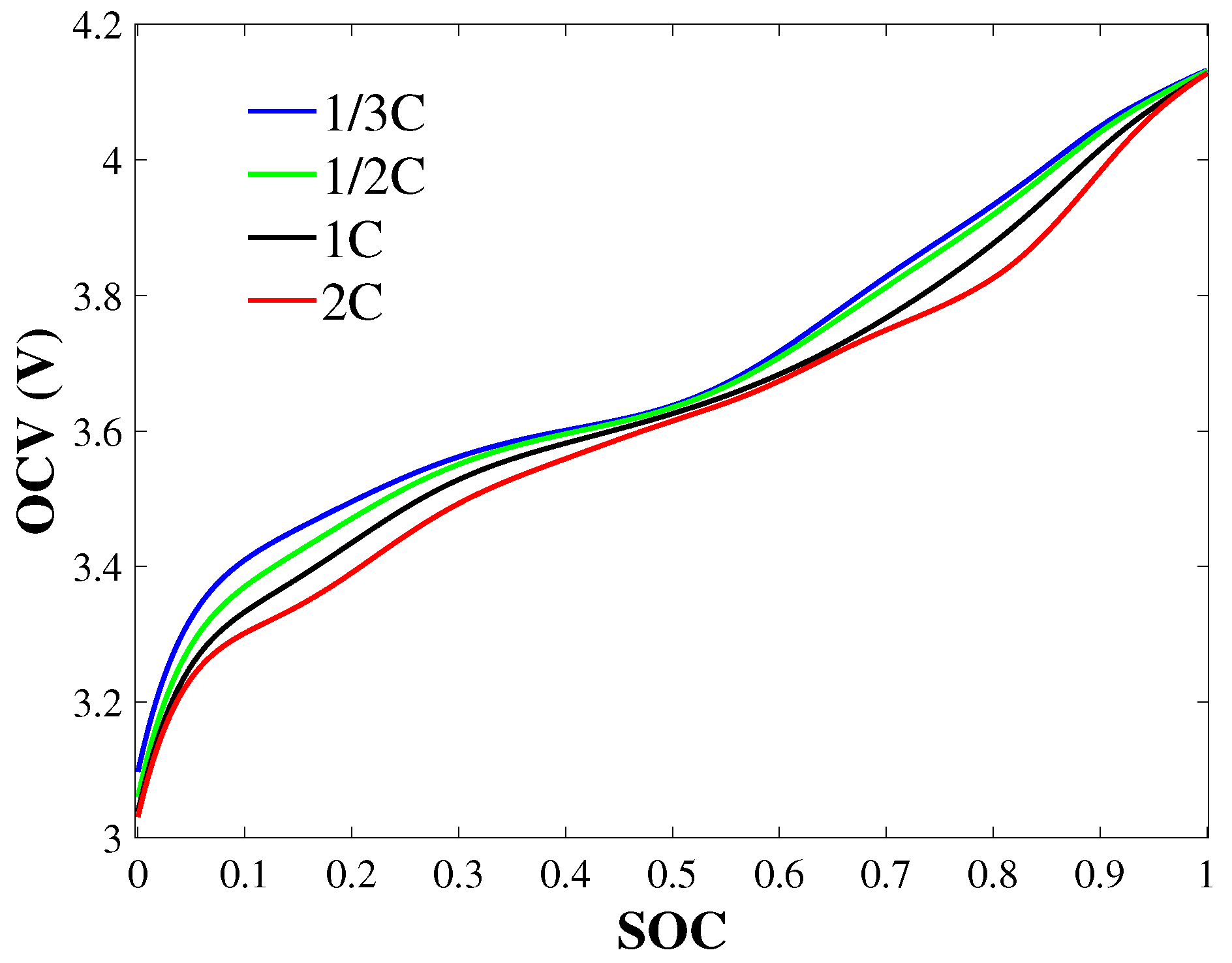
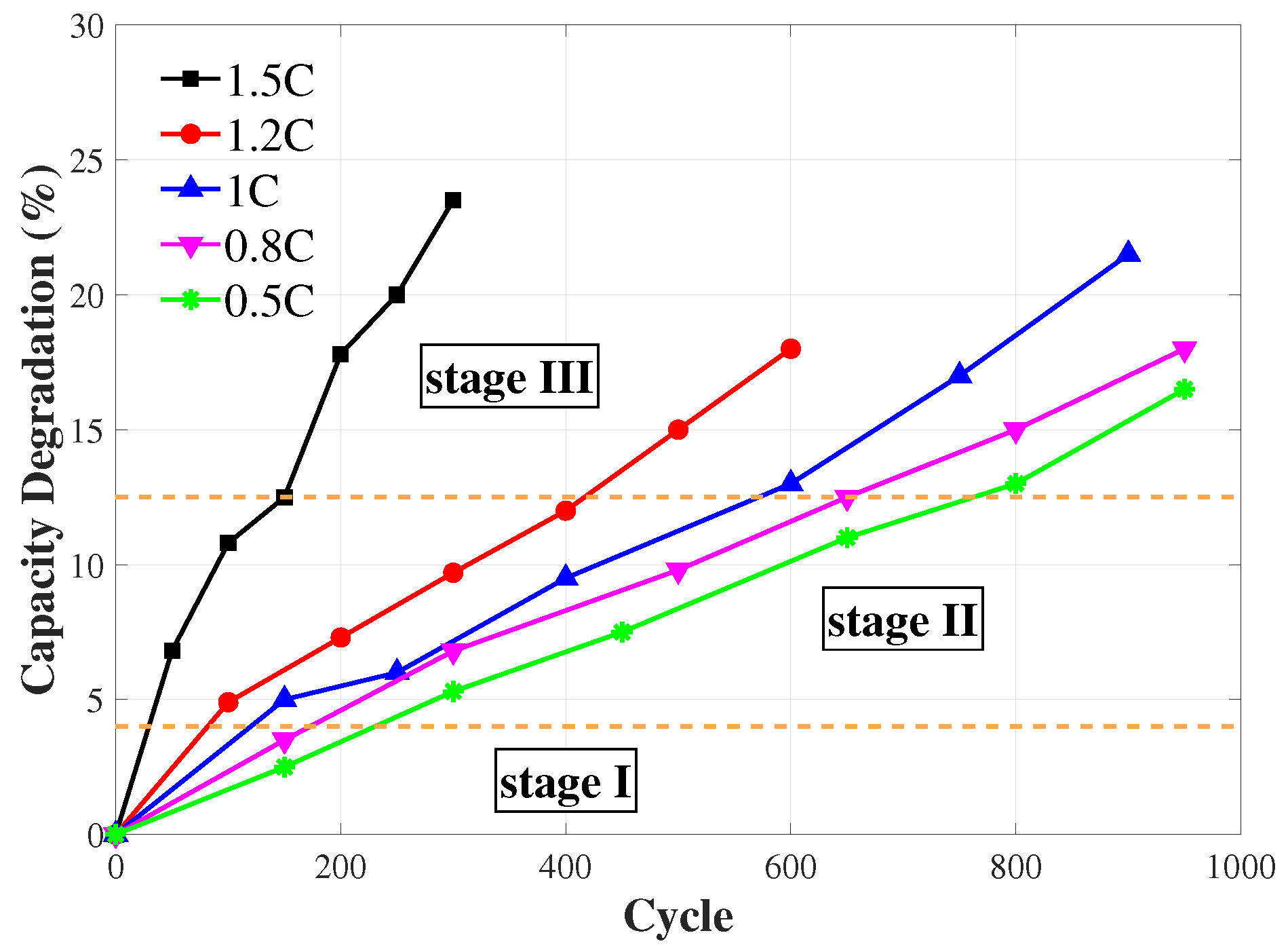
As shown in Figure 1, a single voltage value corresponds to vastly different SOCs under different current rates. Employing a fixed SOC-OCV relationship during dynamic discharge can lead to a significant overestimation of the remaining capacity, posing a major safety hazard for ship navigation. Furthermore, Figure 2 demonstrates that the charge–discharge rate has a direct impact on the rate of battery capacity degradation. The use of a high current rate like 1.5C substantially shortens batteries’ lifespan, which in turn results in higher lifecycle costs for ship navigation. Therefore, the impact of current rates on the estimation results must be taken into consideration when performing the joint estimation of the SOC and SOH; otherwise, it will severely compromise safety and stability during ship navigation.

Based on the above analysis, this article proposes a new SOC and SOH joint estimation method based on an LSTM model integrating a rate-aware attention mechanism (RAAM-LSTM) and SVR model optimized through the GGO algorithm (GGO-SVR). The RAAM addresses the limitation of conventional LSTM in capturing current rate variations, thereby enhancing SOC estimation accuracy under dynamic conditions. Meanwhile, the GGO algorithm optimizes the critical hyperparameters of the SVR model while incorporating physical constraints to suppress unphysical capacity regeneration. In experiments, given the challenges in acquiring full lifecycle data from marine power batteries, the proposed method is validated using the widely adopted non-standard fast-charging, DST and FUDS datasets [32], which effectively replicate the dynamic load characteristics of ship navigation. The main contributions of this article are highlighted below.

(1) A rate-aware attention mechanism is adopted to adjust LSTM hidden states by detecting real-time current variation. This mechanism enhances the model’s focus on rate-varying periods, enabling the more accurate capture of transient battery behavior and significantly improving SOC estimation accuracy compared to conventional LSTM and other neural networks under dynamic current rates.

(2) Building upon the SVR framework, the GGO algorithm and physical constraints are introduced to enhance model performance. The resulting GGO-SVR model substantially improves SOH estimation accuracy, outperforming standard SVR, CNN, and RF methods while maintaining compatibility with real-time deployment through an offline–online decomposition strategy.

(3) A novel SOC and SOH joint estimation method based on RAAM-LSTM and the GGO-SVR model is proposed to improve the accuracy of SOC and SOH estimation under dynamic current rates. The experimental validation confirms that the proposed approach achieves high-precision SOC and SOH estimation.

The remaining content of this article is organized as follows. Section 2 introduces the SOC and SOH joint estimation method. Section 3 describes the data collection and experiment design. Section 4 analyzes and discusses the experimental results. This article concludes with Section 5.

2. Methods

This section describes the principles and derivations of relevant algorithms for SOC and SOH prediction, including the RAAM-LSTM network, SVR, GGO and the general framework of this article.

2.1. Rate-Aware Attention Mechanism–LSTM Network

The fundamental operations of the LSTM network are formulated by the following equations [33]:

$$\left\{\begin{array}{c}\begin{array}{c}{f}_t=\sigma \left(W_{xf}{x}_t+W_{hf}{h}_{t-1}+b_f\right)\\ i_t=\sigma (W_{xi}{x}_t+W_{hi}{h}_{t-1}+b_i)\\ o_t=\sigma (W_{xo}{x}_t+W_{ho}{h}_{t-1}+b_o)\\ {\tilde{C}}_t=\tanh (W_{xC}{x}_t+W_{hC}{h}_{t-1}+b_c)\\ C_t=f_t\otimes C_{t-1}+i_t\otimes {\tilde{C}}_t\\ h_t=o_t\otimes \tanh \left(C_t\right)\end{array}\hfill \end{array}\right.$$

(1)

where $f_t$, $i_t$ and $o_t$ represent the forget, input, and output gates, respectively. $C_t$ represents the cell state which encapsulates long-term memory, and $h_t$ is the hidden state for short-term memory. W represents the input and previous output weight matrices, and b is the bias parameter. The network uses a Sigmoid function ($\sigma$) and Hyperbolic Tangent function (tanh) as activation functions to regulate memory flow. The operator ⊗ denotes element-wise multiplication.

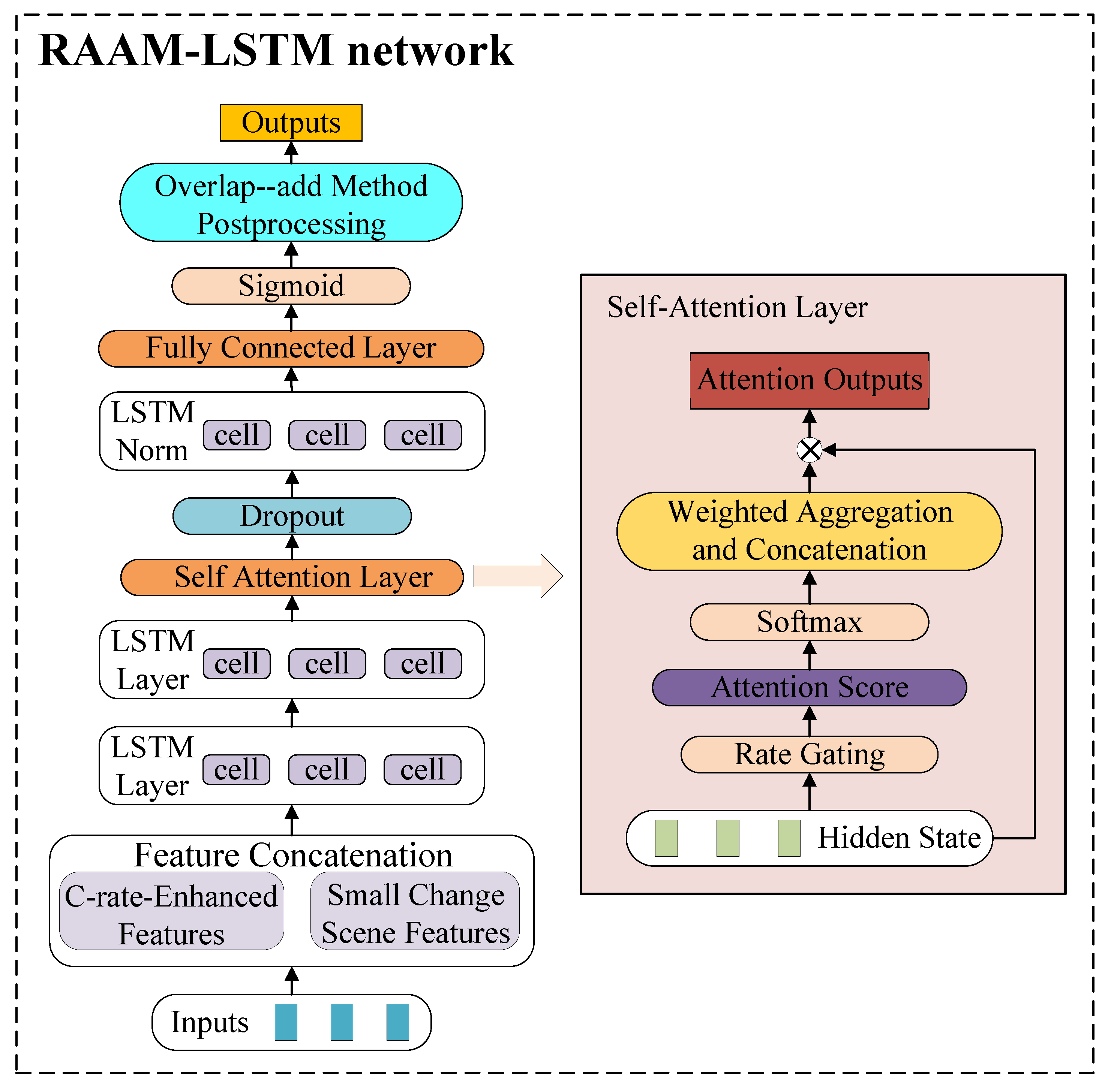
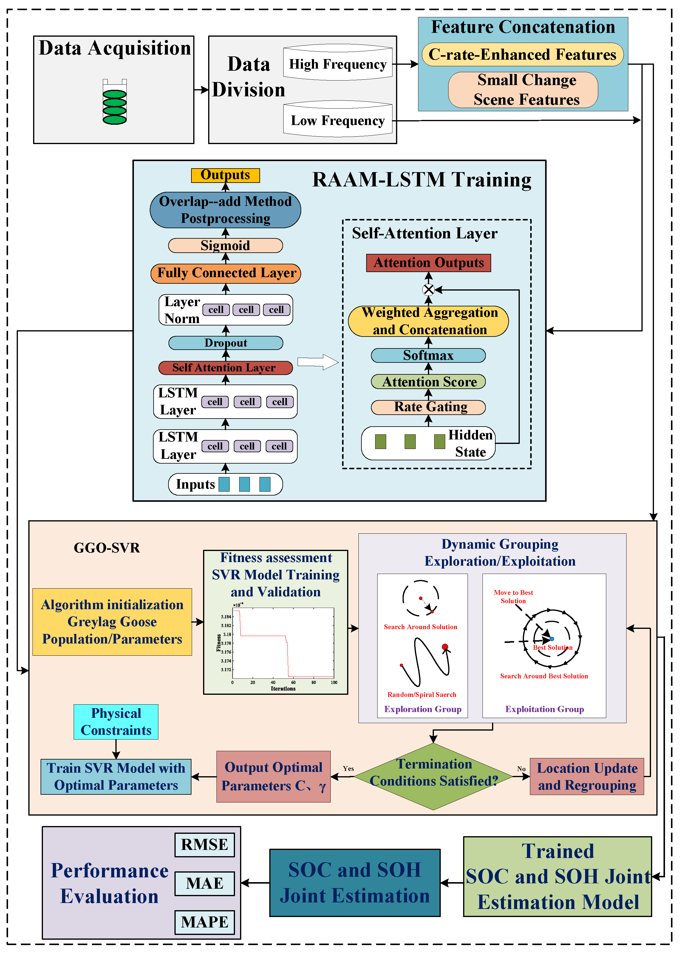
This article proposes an LSTM network with a rate-aware attention mechanism to estimate the SOC of batteries. The proposed RAAM-LSTM network is shown in Figure 3.

The rate-aware attention mechanism proposed in this article is as follows. It can process high- and low-frequency data streams symmetrically, ensuring that both transient dynamics and long-term trends contribute equally to SOC estimation. First, the raw features are categorized into two groups: C-rate-related features and small change scene features. The C-rate-related features are additionally enhanced.

Then, the output features H of the LSTM hidden state are used to generate Query, Key and Value, as shown in the following equation [34]:

$$\left\{\begin{array}{c}{Q}_t=H·W_Q\hfill \\ K_t=H·W_K\hfill \\ V_t=H·W_V\hfill \end{array}\right.$$

(2)

where $W_Q$, $W_K$, and $W_V$ represent the weight matrices for Query, Key and Value.

The rate gating $g_t$ is obtained through rate-related features, which are expressed as follows:

$$RateFeatures=[\left|d_C\right|,\left|d_I\right|,\left|d_{C^2}\right|,\dots ]$$

(3)

$$g_t=\sigma (w_g·RateFeatures+b_g)$$

(4)

By applying $g_t$ to $Q_t$ and $K_t$ through element-wise multiplication, we obtain the rate-enhanced $Q_t^{\prime }$ and $K_t^{\prime }$:

$$Q_t^{\prime }=(1+\alpha ·g_t)\otimes Q_t$$

(5)

$$K_t^{\prime }=(1+\alpha ·g_t)\otimes K_t$$

(6)

where $\alpha$ is used to adjust the weight of rate gating.

Finally, the input is propagated to the softmax layer, which normalizes the attention weights such that each weight value lies between 0 and 1. Following the acquisition of normalized attention weights, they are multiplied by the original input feature matrix, and the results constitute the attention output.

The proposed RAAM-LSTM processes high- and low-frequency data streams symmetrically, ensuring that both transient dynamics and long-term trends contribute equally to SOC estimation. The rate gating factor $g_t$ is designed to maintain symmetry in feature weighting across different current rates.

2.2. Support Vector Regression

SVR is capable of handling nonlinear relationships and high-dimensional datasets. At the same time, it has good generalization ability for small sample datasets. In the specific domain of battery health assessment, SVR demonstrates remarkable efficacy in unraveling the intricate relationships between battery characteristic parameters and the SOH [35].

Through nonlinear mapping, samples are transformed from low-dimensional space to high-dimensional space, which can be defined as follows:

$$f\left(x\right)=\omega ·\varphi \left(x\right)+b$$

(7)

where x is the input data, $\omega$ is the weight, $\varphi \left(x\right)$ is the feature space, and b is the intercept. By introducing the slack variables ${\left\{{\xi }_i\right\}}_{i=1}^n$ and ${\left\{{\xi }_i^{\ast }\right\}}_{i=1}^n$, and according to the principle of risk minimization, the objective function can be formulated as follows:

$$minR\left(\omega ,b,\xi \right)={\displaystyle \frac{1}{2}}{∥\omega ∥}^2+C\sum _i^n\left({\xi }_i+{\xi }_i^{\ast }\right)$$

(8)

$$s.t.=\left\{\begin{array}{c}{y}_i-f\left(x_i\right)\le \epsilon +{\xi }_i\\ f\left(x_i\right)-y_i\le \epsilon +{{\xi }_i}^{\ast }\\ {\xi }_i,{{\xi }_i}^{\ast }\ge 0\end{array}\right.$$

(9)

where ${\xi }_i$ and ${{\xi }_i}^{\ast }$ are the slack variables of the i-th sample. To solve the minimization problem of the objective function, the dual principle is applied by introducing Lagrange multiplier operators ${\alpha }_i$ and ${{\alpha }_i}^{\ast }$. The expression for the SVR model with nonlinear mapping can thus be reformulated as follows:

$$f\left(x\right)=\sum _i^n({\alpha }_i-{{\alpha }_i}^{\ast })K(x_i,x)+b$$

(10)

$K(x_i,x)$ is the kernel function and is expressed as follows:

$$K(x_i,x)=exp(-{\displaystyle \frac{1}{2{\gamma }^2}}{∥x_i-x∥}^2)$$

(11)

To ensure consistency with the physically irreversible nature of battery capacity degradation [36], physical constraints are incorporated into the model to expedite the recession of capacity regeneration phenomena. Let the original predicted sequence be denoted as ${\widehat{S}}_i(i=1,2,\dots ,n)$ and the estimated sequence that satisfies the physical constraints be denoted as $S_i$. The constraint process can be summarized as the following four sequentially executed steps, with its mathematical formulation provided below:

Step 1. Press capacity regeneration

Set the regeneration threshold to 0.02. If $S_i^{\left(1\right)}>S_{i-1}+0.02$, then

$$S_i^{\left(2\right)}=S_{i-1}+0.3·(S_i^{\left(1\right)}-S_{i-1})$$

(12)

If the regeneration amplitude exceeds 0.05, a forced rollback is applied:

$$S_i^{\left(2\right)}=S_{i-1}$$

(13)

Step 2. Adaptive constraint based on the trend in true values

If the true value sequence $T_i$ is available and the actual increase exceeds a tolerance of 0.01, the predicted value is constrained to follow within a limited range:

$$S_i^{\left(3\right)}=min(S_i^{\left(2\right)},S_{i-1}+0.01)$$

(14)

Step 3. Maximum decay rate constraint

To prevent an excessively large single-step decrease, the maximum decay rate is set to 0.08:

$$S_i^{\left(4\right)}=max(S_i^{\left(3\right)},S_{i-1}-0.08)$$

(15)

Step 4. Local smoothing

Weighted smoothing is applied to capacity regeneration regions, while simple averaging is used for non-regeneration regions:

If $S_i^{\left(4\right)}>S_{i-1}^{\left(4\right)}$ and $S_i^{\left(4\right)}>S_{i+1}^{\left(4\right)}$, then five-point weighted averaging is applied:

$$S_i^{\left(5\right)}=0.1S_{i-2}^{\left(4\right)}+0.2S_{i-1}^{\left(4\right)}+0.4S_i^{\left(4\right)}+0.2S_{i+1}^{\left(4\right)}+0.1S_{i+2}^{\left(4\right)}$$

(16)

Otherwise, three-point weighted averaging is applied, with boundary points handled using available neighbors:

$$S_i^{\left(5\right)}={\displaystyle \frac{S_{i-1}^{\left(4\right)}+S_i^{\left(4\right)}+S_{i+1}^{\left(4\right)}}{3}}$$

(17)

2.3. Greylag Goose Optimization

The parameter selection of the penalty factor C in Equation (8) and the kernel parameter $\gamma$ in Equation (11) is formulated as a nonconvex and multimodal optimization problem. To solve it efficiently, this article adopts the GGO algorithm. The specific workflow is detailed below [37].

Step 1. Population initialization. The population is randomly initialized across the feasible solution space, representing the positions of individual greylag geese in the first generation. This process is described as follows:

$$x_{i,j}^0=a_j+\mathrm{rand}·(b_j-a_j),\hspace{1em}i=1,2,\dots ,n,\hspace{1em}j=1,2,\dots ,m$$

(18)

where $x_{i,j}^0$ denotes the initial position of the i-th individual in the j-th dimension, and $a_j$ and $b_j$ represent the lower and upper bounds of the solution space, respectively. n is the population size, m is the dimensionality, and $rand$ is a random number uniformly distributed in $[0,1]$.

Step 2. Fitness evaluation. Each individual’s fitness value is calculated using the function $F_n$, and the current optimal individual position $x^{\ast }$ along with its corresponding fitness value is recorded.

Step 3. Dynamic grouping. The population is divided into an exploration group and exploitation group. Initially, each group accounts for 50% of the population. Subsequently, the grouping is dynamically adjusted based on the update status of the optimal solution during the iterative process: if the optimal solution remains unchanged for three consecutive iterations, the size of the exploration group is increased to enhance global exploration capability and avoid entrapment in local optima.

Step 4. Exploration operation. The exploration group is responsible for searching new regions within the solution space to prevent premature convergence. The position update strategy is selected according to the following condition:

When $\left|A\right|<1$, the individuals move toward the current optimal individual:

$$X(t+1)=X^{\ast }\left(t\right)-A·|C·X^{\ast }\left(t\right)-X\left(t\right)|$$

(19)

where $A=2a·r_1-a, C=2r_2$, and a decreases linearly from 2 to 0.

When $\left|A\right|\ge 1$, exploration is performed using three randomly selected individuals:

$$X(t+1)={\omega }_1{X}_{\mathrm{paddle}1}+z·{\omega }_2(X_{\mathrm{paddle}2}-X_{\mathrm{paddle}3})+(1-z)·{\omega }_3(X-X_{\mathrm{paddle}1})$$

(20)

where $z=1-{(t/t_{max})}^2$, and ${\omega }_1,{\omega }_2,{\omega }_3\in [0,2]$.

When $r_3\ge 0.5$, a spiral search strategy is adopted:

$$X(t+1)={\omega }_4|X^{\ast }\left(t\right)-X\left(t\right)|e^{bl}cos\left(2\pi t\right)+\left[2{\omega }_1(r_4+r_5)\right]X^{\ast }\left(t\right)$$

(21)

where b is a constant, $l\in [-1,1]$, and ${\omega }_4\in [0,2]$.

Step 5. Exploitation operation. The exploitation group is responsible for conducting a refined search in the vicinity of the current optimal solution to enhance solution quality. Its update methods include the following:

Guidance based on the positions of three sentry individuals. The final position is obtained by averaging the three positions:

$$\left\{\begin{array}{c}{X}_1=X_{\mathrm{sentry}1}-A_1·|C_1{X}_{\mathrm{sentry}1}-X|\hfill \\ X_2=X_{\mathrm{sentry}2}-A_2·|C_2{X}_{\mathrm{sentry}2}-X|\hfill \\ X_3=X_{\mathrm{sentry}3}-A_3·|C_3{X}_{\mathrm{sentry}3}-X|\hfill \end{array}\right.$$

(22)

If $t\%2\ne 0$, neighborhood search is performed:

$$X(t+1)=X\left(t\right)+D(1+z)·\omega ·(X-X_{\mathrm{flock}1})$$

(23)

where D is a random direction vector.

If the fitness value of each updated individual is superior to the original, it is replaced; otherwise, the original individual is retained. Meanwhile, an elite strategy is adopted to ensure that the optimal individual of each generation is not lost. This process is repeated until the termination condition is satisfied. Finally, the global optimal solution and its corresponding fitness value are output.

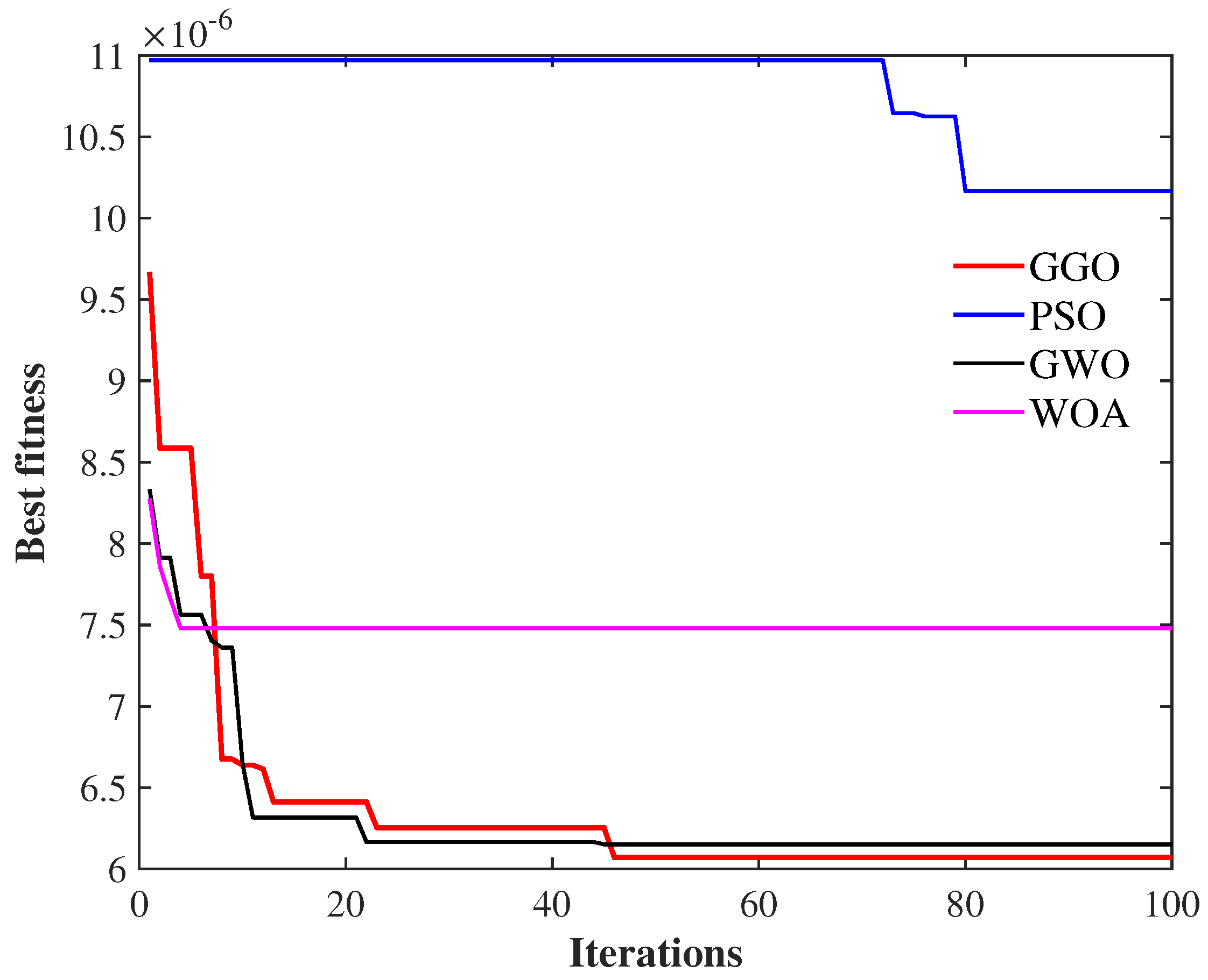
To justify the selection of the GGO algorithm, its optimization performance was compared against other typical metaheuristic algorithms, including Particle Swarm Optimization (PSO), the Gray Wolf Optimizer (GWO), and the Whale Optimization Algorithm (WOA). As illustrated in Figure 4, the fitness convergence curves demonstrate that GGO exhibits superior convergence speed and achieves higher solution quality. Specifically, GGO avoids premature convergence to local optima more effectively than PSO and the WOA and reaches a lower final fitness value than the GWO. Furthermore, compared to traditional grid or random search constraints, the GGO algorithm exhibits greater robustness on irregular response surfaces. Moreover, unlike gradient-based methods, it is derivative-free and less sensitive to noise in the validation metric. Consequently, GGO facilitates highly efficient, globally oriented hyperparameter tuning for the SVR model, leading to improved generalization capability in SOH estimation, particularly on small- to medium-sized datasets.

2.4. Framework of SOC and SOH Estimation

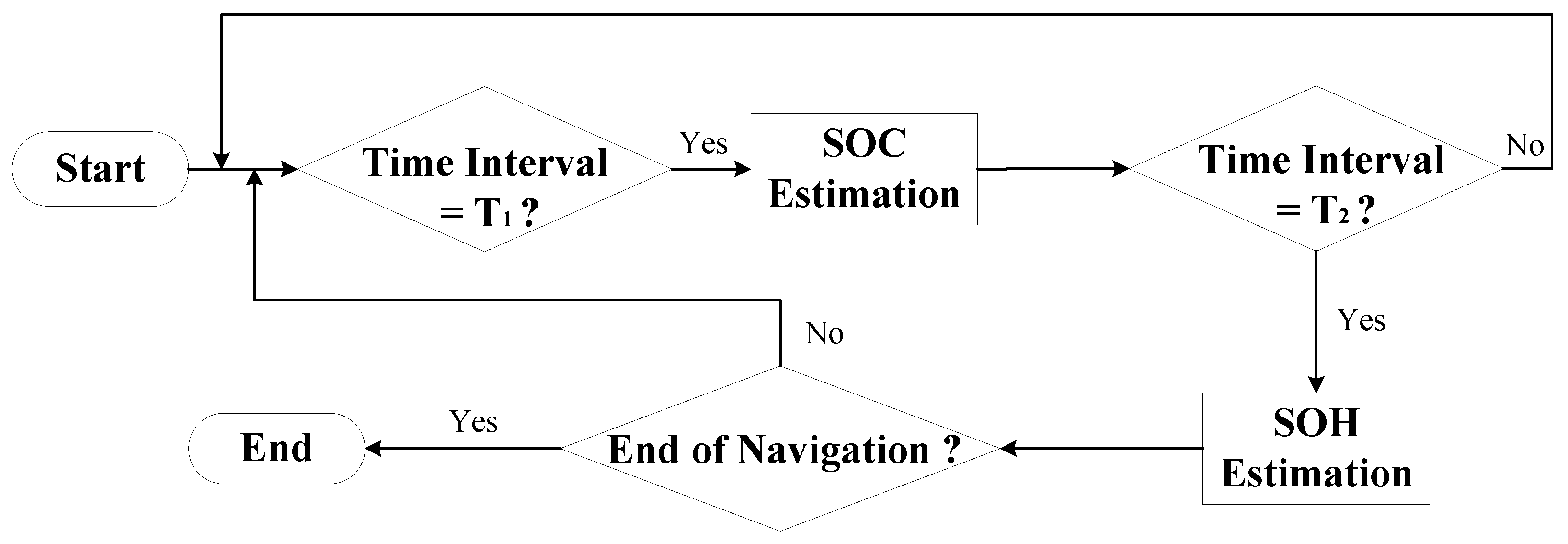
The implementation procedure of the proposed SOC and SOH estimation based on RAAM-LSTM and SVR with GGO is illustrated in Figure 5. The whole process is mainly divided into five steps: data acquisition and division, feature concatenation, RAAM-LSTM network training, GGO-SVR model training, and SOC and SOH joint estimation. First, the acquired battery data is separated into a high-frequency stream and a low-frequency stream. Subsequently, the high-frequency data undergoes current rate feature enhancement, combined with minor variation scenarios, and is then fed into the RAAM-LSTM network for training. Concurrently, the enhanced features and SOC are used to train the SVR model, whose parameters are optimized by the GGO algorithm. A flowchart of the multi-timescale joint state estimation process is shown in Figure 6. Finally, the trained models for estimating the SOC and SOH are obtained, and their estimation performance is validated.

To facilitate real-time deployment on practical BMSs with limited computational capabilities, the proposed framework adopts an offline–online decomposition strategy, separating computationally intensive tasks from real-time execution. In the offline phase, model training and hyperparameter optimization are performed on the high-performance computing platform. The RAAM-LSTM network is pre-trained offline using the historical dynamic current rate dataset. At the same time, the optimal SVR parameters (C and $\gamma$) are optimized by the dynamic grouping and iterative search of the GGO algorithm. In the online phase, only the trained RAAM-LSTM network and SVR model with fixed optimal parameters are deployed to the embedded BMS, and the real-time operation process only involves lightweight forward-pass inference.

3. Data Collection and Experiment Design

In the DC distribution network of marine power systems, the bus voltage is maintained at a constant level [38]. Although the terminal voltage of battery cells decreases during discharge, it must be stepped up to the bus voltage via a DC–DC converter. Variations in ship load power lead to changes in the output current of the battery system, which in turn alters the number of battery modules connected to the bus. As a result, from the perspective of the individual cell, it can be regarded as operating under a quasi-constant voltage condition over extended periods. In addition, to preserve the battery’s health and useful life, it is usually operated exclusively through shore-based charging or battery swapping. Under this operational paradigm, the battery begins each voyage at a full or near-full state of charge. During navigation, it undergoes intermittent but sustained discharge until reaching a lower threshold of 20%, after which it is taken offline and enters a rest state. The two characteristics indicate that the operational profile of marine power battery systems exhibits a marked contrast to those of electric vehicles and stationary energy storage stations.

Due to the difficulties in acquiring full lifecycle data from marine power batteries, this article employs publicly available, laboratory-grade battery datasets. Despite the differences, the load profiles of the non-standard fast-charging test, DST and FUDS developed for electric vehicle testing exhibit strong similarities with typical marine operating conditions. The typical navigation of a ro-ro vessel comprises five distinct operational phases. The stepwise increase in current rates during non-standard fast-charging experiments shares a similarity with progressive loading during cargo handling operations. During departure, the rapid acceleration demand mirrors the high-current transients in FUDS. In open-water cruising, steady propulsion is superimposed with periodic wave-induced fluctuations and auxiliary equipment cycling, closely resembling the platform-plus-pulse structure of DST. Approaching the port, continuous deceleration and berthing maneuvers produce regenerative charging and random power variations analogous to the FUDS deceleration phases. Finally, during the docking phase, auxiliary loads create stepwise patterns consistent with DST pulsed sequences. Therefore, validation under DST and FUDS conditions comprehensively captures the full spectrum of dynamic loads encountered in ferry operations, providing a representative basis for evaluating the proposed method in marine applications.

The battery data used in this section comprise the fast-charging data of lithium batteries obtained from non-standard charging experiments, as well as data from the Center for Advanced Life Cycle Engineering (CALCE) at the University of Maryland. To obtain the fast-charging data, a series of CCCV cycles with incrementally increasing C-rates was executed to characterize performance under high-rate conditions. Following this, capacity fade was evaluated through 1C CCCV baseline tests. In the CALCE experiments, a cylindrical INR 18650R cell with a nominal capacity of 2.0 Ah was employed. Following a complete charge via a standard method, the sample was subjected to a rest period to dissipate polarization. The practical testing data comes from the DST and FUDS at temperatures of 25 °C and 45 °C. 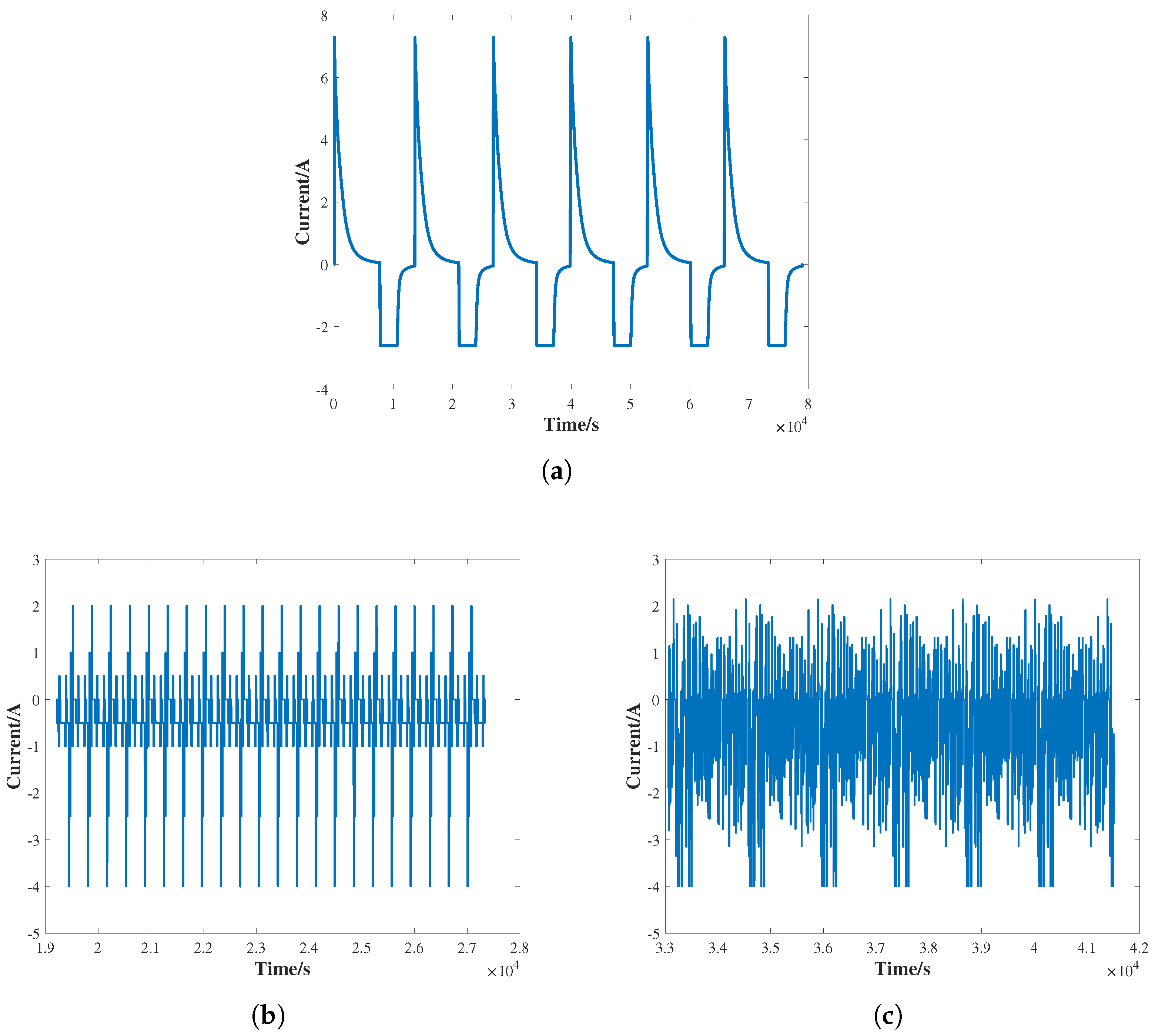Initially, $SO{C}_0$ is established at 0.8. To provide a clear visualization of the highly dynamic load characteristics, the current profiles of the non-standard fast-charging test, DST and FUDS testing cycles are illustrated in Figure 7.

The estimation accuracy of this article is evaluated using the root mean square error (RMSE), mean absolute error (MAE), and mean absolute percentage error (MAPE), which are given in (24)–(26).

$$\mathrm{RMSE}=\sqrt{{\displaystyle \frac{1}{N}}\sum _{i=1}^N{\left({\widehat{y}}_i-y_i\right)}^2}$$

(24)

$$\mathrm{MAE}={\displaystyle \frac{1}{N}}\sum _{i=1}^N|{\widehat{y}}_i-y_i|\times 100$$

(25)

$$\mathrm{MAPE}={\displaystyle \frac{1}{N}}\sum _{i=1}^N|{\displaystyle \frac{{\widehat{y}}_i-y_i}{y_i}}|\times 100$$

(26)

where ${\widehat{y}}_i$ represents the prediction results of the SOC or SOH, $y_i$ denotes the actual value, and N stands for the number of samples.

4. Results and Discussion

It is pertinent to clarify the rationale behind our experimental comparison strategy before presenting the results. While this paper proposes a joint estimation framework, we deliberately chose not to perform a direct end-to-end comparison against other integrated joint estimation models from the literature. Instead, we evaluate our proposed SOC and SOH joint estimation model against well-established baseline algorithms in their respective domains (e.g., LSTM, BiLSTM for SOC; SVR, CNN for SOH). This ‘divide and conquer’ approach is methodologically crucial for isolating and rigorously validating the specific contributions of our core innovations. By doing so, we can clearly attribute performance gains to our specific architectural and algorithmic enhancements, such as the RAAM and the GGO algorithm, rather than ambiguously attributing them to the overall performance of a monolithic joint estimation framework. This strategy ensures a clear and fair demonstration of the effectiveness of each component of our proposed solution.

4.1. Performance Evaluation Under Dynamic Current Rate Conditions

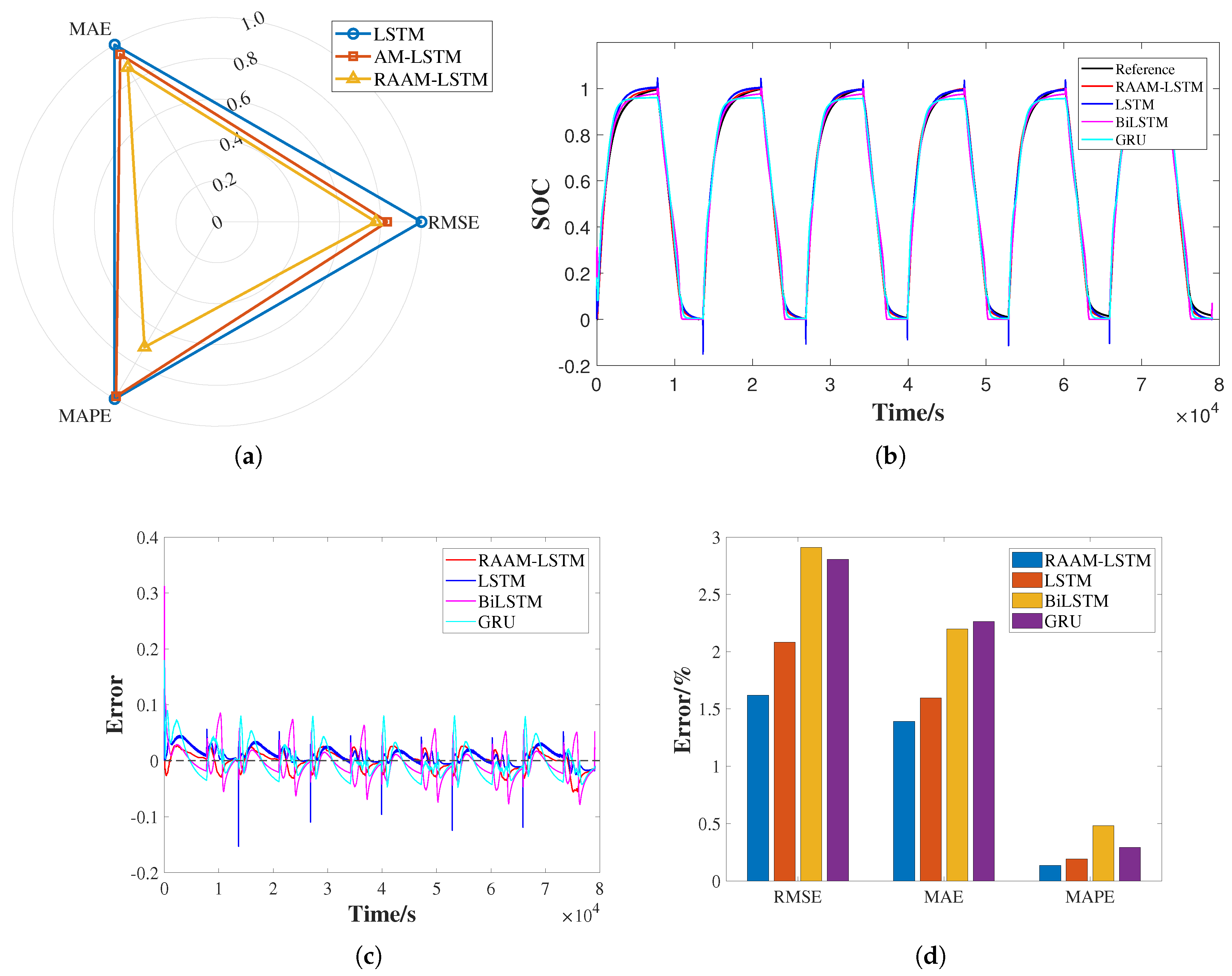
In order to verify the specific contribution of rate gating in the proposed RAAM, we conducted an ablation experiment. We additionally implemented and evaluated an LSTM model with a standard attention mechanism. The experimental results are shown in Figure 8a. The results show that compared with the LSTM model, the RMSE value of the AM-LSTM model is improved by 16.68%, which indicates that the introduction of the attention mechanism itself is beneficial to capture the dependence of time series. However, the proposed RAAM-LSTM model achieves the optimal performance, and its error is further reduced by 5.61% compared with the AM-LSTM model. This result strongly proves that the RAAM we designed can effectively use the current rate change information to dynamically adjust the focus of the model so as to achieve more accurate SOC estimation under dynamic conditions. This clearly isolates and verifies the fact that the rate gating mechanism is the key innovation for improving the performance of the model. The SOC estimation results of non-standard fast-charging data are represented in Figure 8b, with the corresponding error analysis depicted in Figure 8c. Detailed performance metrics are visually represented in Figure 8d for comprehensive evaluation.

Through validation, it is observed that the LSTM model exhibits an RMSE of 2.08%, the BiLSTM model achieves an RMSE of 2.91%, and the GRU model attains an RMSE of 2.81%, all producing relatively accurate SOC estimates. However, due to the influence of varying current rates in non-standard charging processes, these models demonstrate notable fluctuations and compromised robustness in SOC estimation. Conversely, the RAAM-LSTM model maintains significantly better stability under such dynamic current conditions, improving the performance of the RMSE by 22.11%, 44.67%, and 42.70% compared to LSTM, Bilstm, and the GRU. The MAEs of the RAAM-LSTM, LSTM, BiLSTM, and GRU models are recorded at 1.39%, 1.60%, 2.22%, and 2.26%, respectively. The MAPE value achieved by RAAM-LSTM reaches 0.14%, which is reduced by 26.32%, 70.83%, and 51.72% relative to LSTM, BiLSTM, and the GRU. The results, hence, demonstrate that the estimation effect of RAAM-LSTM is better than that of LSTM without the RAAM, which verifies the effectiveness of the rate awareness attention mechanism.

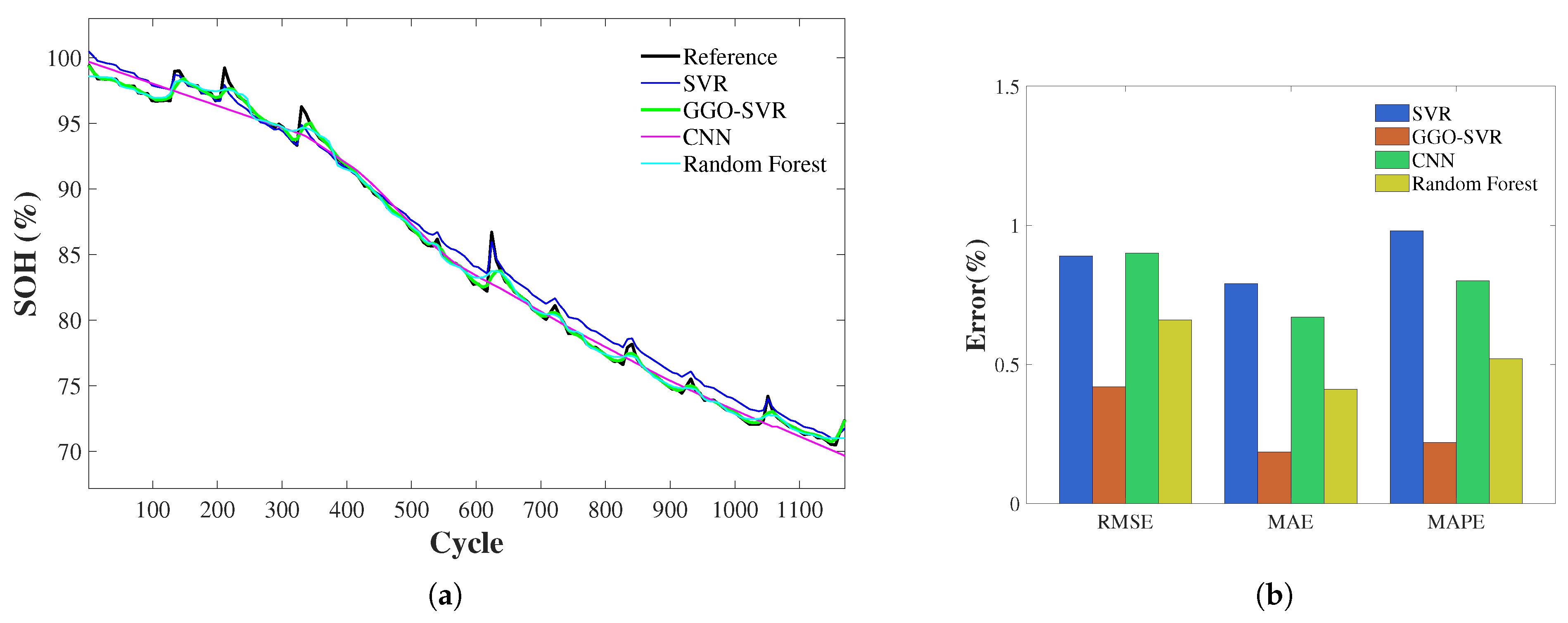
To further validate the effectiveness of the proposed SOH estimation method, this article compares the proposed method with three conventional SOH estimation methods, including SVR, a CNN, and RF. To ensure the fairness of comparison, the network hyperparameters of SVR, the CNN, and RF are set to be consistent with the proposed method. The SOH estimation results of the four methods are shown in Figure 9.

The RMSE values of SVR, GGO-SVR, the CNN, and RF reach 0.89%, 0.42%, 0.9%, and 0.66%. For the proposed method, the MAE is reduced by 77.22%, 73.13%, and 56.10%, compared to SVR, the CNN, and RF respectively. At the same time, the MAPE for the proposed method is reduced by 77.55%, 72.5%, and 57.69%. Furthermore, the proposed method demonstrates a faster correction of the nonphysical positive drift in the estimated SOH, which is inconsistent with the unidirectional and irreversible capacity degradation mechanism of lithium-ion batteries. Therefore, this article used the GGO-SVR model for SOC and SOH joint estimation.

4.2. Generalization Validation Across Different Testing Cycles

In this section, the DST and FUDS testing data at 25 °C are used to validate the generalization of the proposed method. The SOC and SOH joint estimation results for the two conditions are depicted in Figure 10, Figure 11, Figure 12 and Figure 13. Since battery aging is a gradual process, the SOH variation within a single cycle is negligible and can be treated as zero.

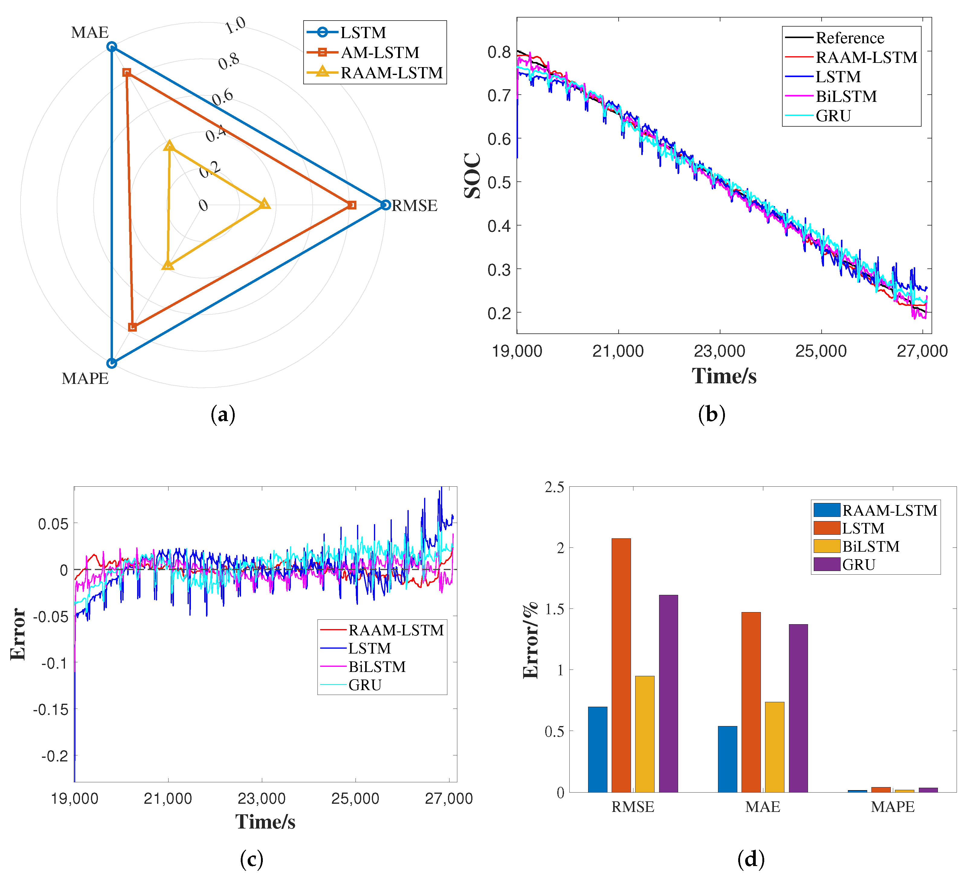
Figure 10 shows the comparison results of the SOC estimated by the proposed method and LSTM, BiLSTM, and the GRU. The ablation results are shown in Figure 10a. The results show that, compared with the LSTM model with the same attention mechanism, the RAAM-LSTM model achieves lower estimation error and higher accuracy through its unique rate sensing gating function. As shown in Figure 10b,c, the proposed method can accurately estimate the SOC. Compared to the LSTM, BiLSTM and GRU models, it exhibits reduced fluctuations in its estimates. The RMSE values for RAAM-LSTM, LSTM, BiLSTM and the GRU are 0.70%, 2.07%, 0.95% and 1.61%, respectively. The MAE for the proposed method is reduced by 63.26%, 27.03%, and 60.58%. Additionally, the MAPE for the proposed method is reduced by 61.64%, 16.18%, and 57.10%.

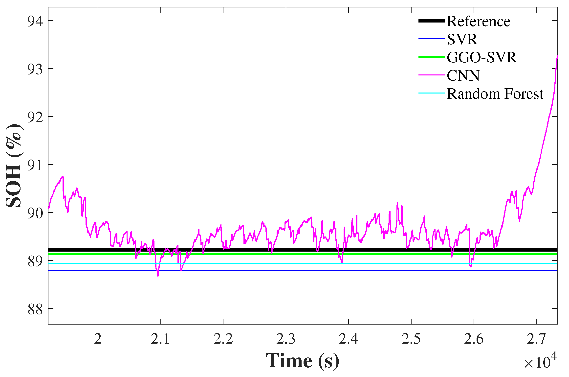
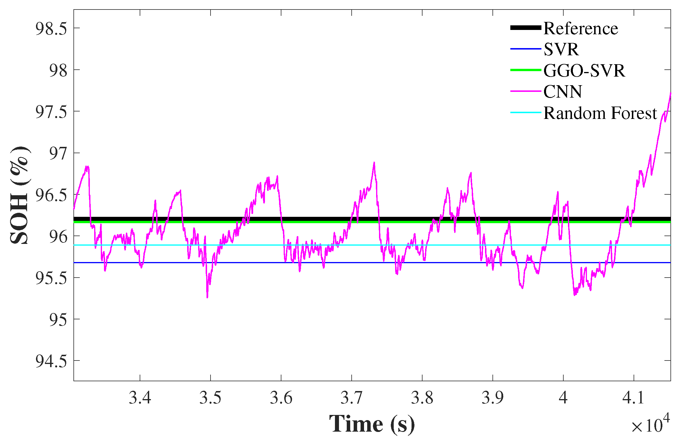
The joint estimation results of the SOH are presented in Figure 11. As observed, the proposed method provides estimates that are the closest to the true value, whereas the CNN exhibits the most volatile estimation profile. The corresponding performance metrics for all methods are summarized in

Table 1. Comparison results of SOH estimation at 25 °C under DST conditions.

	SVR	GGO-SVR	CNN	RF
RMSE (%)	1.12	0.23	1.96	0.75
MAE (%)	1.12	0.23	2.21	0.75
MAPE (%)	0.48	0.1	0.96	0.32
TIME (s)	0.92	0.91	13.20	1.76

. It takes 6.3 s for the GGO algorithm to optimize SVR parameters offline. Compared to SVR, the CNN, and RF, the GGO-SVR model improves estimation accuracy by 79.46%, 88.26%, and 69.33%, respectively.

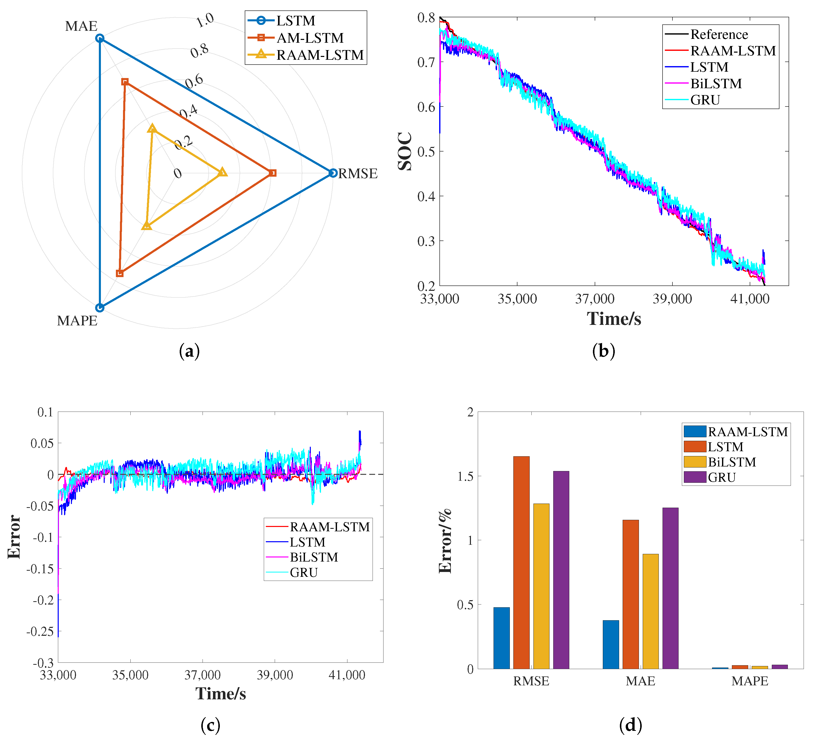
The results of SOC estimation under FUDS conditions are shown below. An ablation study is conducted by introducing an AM-LSTM model to isolate the contribution of the rate-aware mechanism in Figure 12a. While the AM-LSTM model shows some improvement over the baseline LSTM, RAAM-LSTM achieves a significantly lower RMSE, MAE and MAPE. As illustrated in Figure 12b,c, the proposed RAAM-LSTM method demonstrates superior performance to the baseline LSTM, BiLSTM and GRU, exhibiting reduced error fluctuations and a closer proximity to the reference. The RMSE value of SOC estimation under FUDS conditions at 25 °C reaches 0.47%, which is reduced by 70.91%, 62.5% and 68.83% compared to the LSTM, BiLSTM and GRU models. Additionally, the values of the MAE and MAPE are reduced by 67.83% and 60% compared to LSTM without the RAAM respectively. The comparison results of joint SOH estimation are shown in Figure 13 and

Table 2. Comparison results of SOH estimation at 25 °C under FUDS conditions.

	SVR	GGO-SVR	CNN	RF
RMSE (%)	1.36	0.09	1.00	0.81
MAE (%)	1.36	0.09	0.30	0.81
MAPE (%)	0.55	0.04	0.12	0.32
TIME (s)	1.10	1.17	15.00	1.93

. The RMSE values for the proposed method, SVR, CNN, and RF are 0.09%, 1.36%, 1.00%, and 0.81%. This demonstrates that the proposed method has the highest estimation accuracy.

Hence, based on the above results under both DST and FUDS cycles, the proposed method demonstrates consistent and precise estimation capabilities for both the SOC and SOH. The RAAM-LSTM model achieves accurate SOC tracking with minimal error fluctuations across different dynamic current rates, while the GGO-SVR model provides stable and reliable SOH estimates closest to the reference. These results collectively confirm the method’s accuracy and generalization ability in performing joint state estimation under varied operating conditions.

4.3. Generalizability Assessment Under Various Temperatures

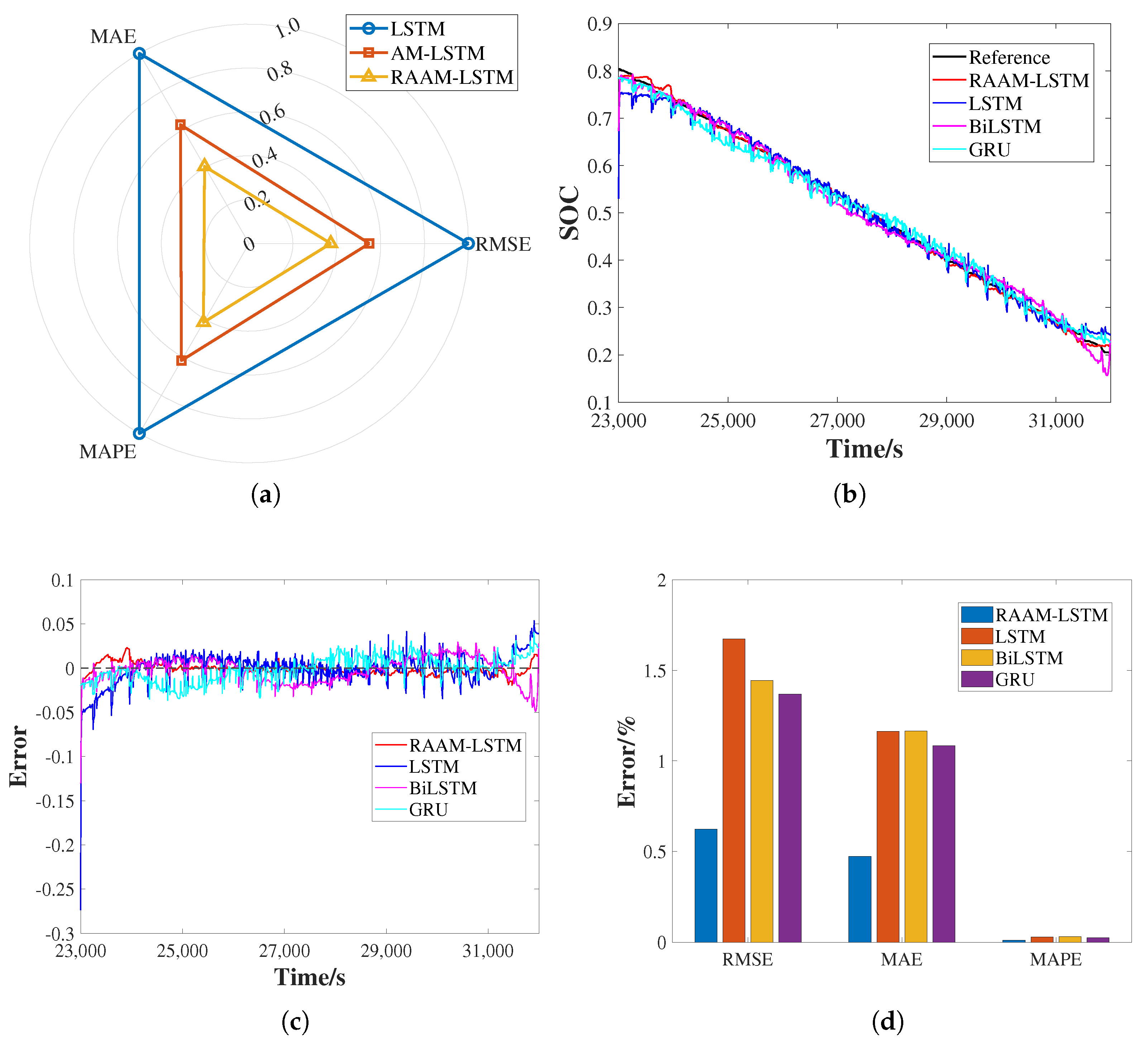
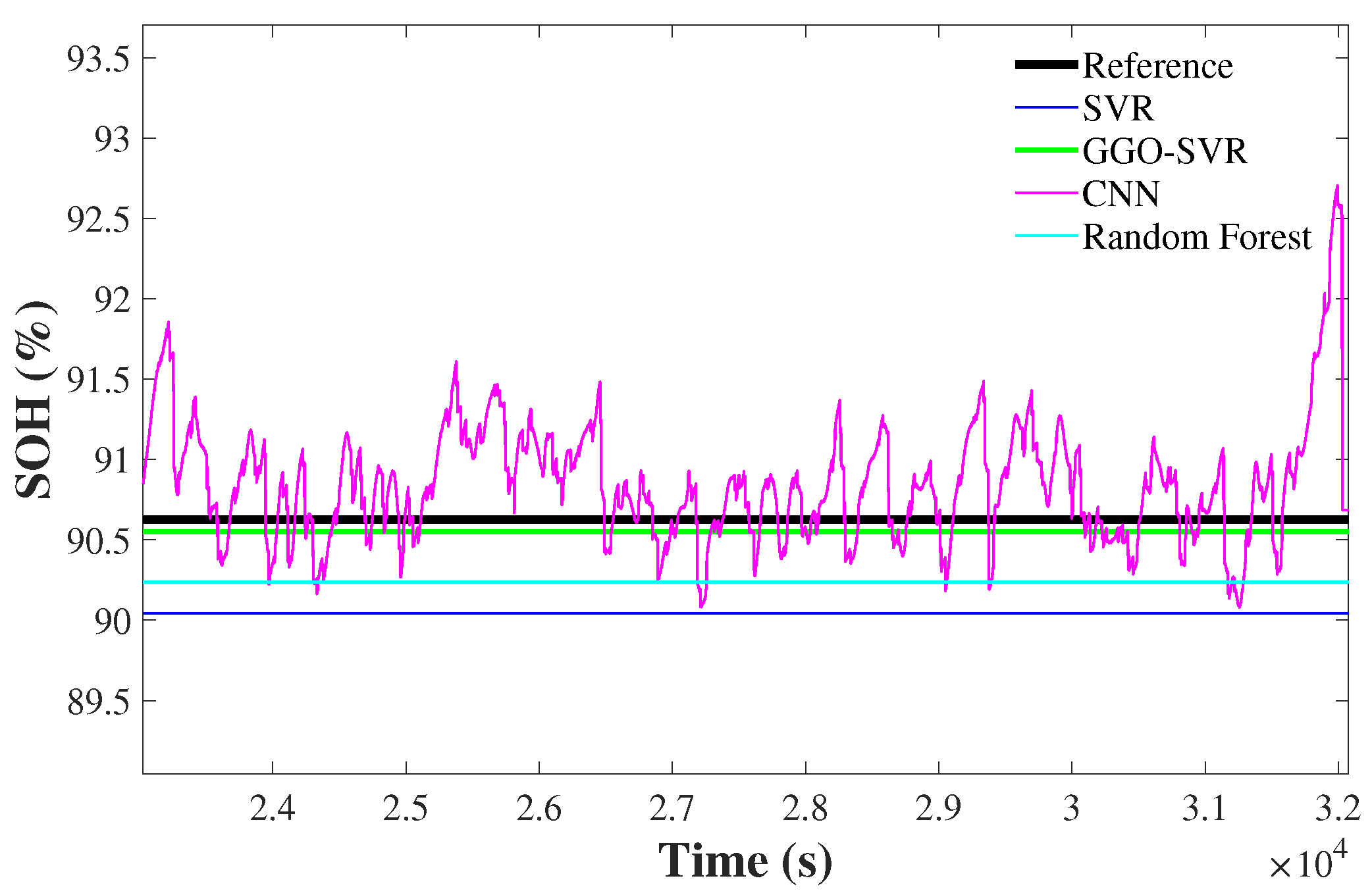
A comparative analysis was performed to further investigate the efficacy of the proposed method across temperatures, utilizing the DST profile at 45 °C. The SOC and SOH estimation results of the method are shown in Figure 14 and Figure 15.

To rigorously evaluate the specific contribution of the rate-aware component, Figure 14a present the results from an ablation study, which includes an AM-LSTM model as a control. Figure 14b,c show the comparison results of the SOC estimated by the proposed RAAM-LSTM method and LSTM, BiLSTM, and the GRU. The RMSE values for them are 0.62%, 1.67%, 1.44% and 1.37%, respectively. The ablation results further confirm that while AM-LSTM offers an improvement over the baseline LSTM, the proposed RAAM is the key factor that grants the model enhanced precision under elevated temperatures and dynamic conditions. The MAE for the proposed method is reduced by 59.48%, 59.36% and 56.48% compared to LSTM, BiLSTM and the GRU. Additionally, the MAPE for the proposed method is reduced by 58.61%, 61.70% and 52.92%.

The results of SOH estimation are given in Figure 15 and

Table 3. Comparison results of SOH estimation at 45 °C under DST condition.

	SVR	GGO-SVR	CNN	RF
RMSE (%)	1.52	0.20	0.73	1.01
MAE (%)	1.52	0.20	0.59	1.01
MAPE (%)	0.64	0.08	0.25	0.42
TIME (s)	1.03	0.95	14.60	1.96

. For SOH joint estimation at 45 °C, the RMSE values for SVR, GGO-SVR, the CNN and RF are 1.52%, 0.20%, 0.73%, and 1.01%, respectively. The proposed GGO-SVR model improves the accuracy by 86.84%, 72.60%, and 80.20% compared to SVR, the CNN, and RF.

In summary, the experimental results under the DST profile at 45 °C consistently validate the effectiveness of the proposed joint estimation method, compared with the test data at 25 °C. The high estimation accuracy maintained across this temperature range demonstrates its notable thermal robustness, which is a crucial attribute for practical BMS applications in varying environmental conditions.

4.4. Critical Discussion on Generalizability to Real Marine Systems

While the proposed RAAM-LSTM and GGO-SVR framework demonstrated superior accuracy and thermal robustness on laboratory datasets, its transition to real-world marine battery systems presents several multifaceted challenges that warrant critical discussion.

One key challenge lies in the fact that operational and environmental conditions in marine applications are profoundly more complex. Although DST and FUDS cycles emulate certain navigation phases, they do not fully capture the stochastic and harsh stressors encountered at sea, such as high humidity and salinity and persistent mechanical vibrations. Moreover, the uniform thermal conditions (25 °C and 45 °C) in our validation contrast with the uneven spatial temperature distribution found in large-scale battery packs within ship engine rooms, which can aggravate localized polarization and inter-cell inconsistencies.

Another critical aspect concerns the fact that the aging mechanisms in marine batteries diverge significantly from those of typical electric vehicles. Marine vessels often undergo prolonged berthing and anchorage, making calendar aging a dominant factor alongside cycle aging. Consequently, capacity degradation models trained solely on continuous cycling data may fail to accurately capture the fade induced by long-term resting states under maritime climatic conditions.

A further difference stems from battery chemistry. Real-world marine systems predominantly utilize large-capacity Lithium Iron Phosphate (LiFePO4) batteries for their superior thermal stability. These batteries exhibit flatter OCV-SOC plateaus compared to the INR 18650R cells used in the CALCE dataset, posing a challenge for accurate SOC estimation. To bridge this gap, future work must focus on generalizing the proposed offline–online strategy. This can be achieved by incorporating transfer learning or online adaptive fine-tuning, which would allow the pre-trained models to adapt to specific marine aging dynamics and complex multi-physics variations using limited real-world operational data. Such adaptations are crucial for ensuring the high reliability of the proposed framework in practical maritime navigation.

5. Conclusions

To improve the accuracy of SOC and SOH estimation for lithium-ion batteries under dynamic current rates, this article proposes a novel SOC-SOH joint estimation method, integrating an RAAM-LSTM network for SOC estimation and an SVR model optimized by the GGO algorithm for SOH estimation. In this method, the RAAM adjusts the weights of LSTM hidden states by detecting current variations, thereby enhancing feature extraction capability during dynamic periods. Concurrently, the GGO algorithm is employed to optimize the critical hyperparameters of the SVR model, significantly improving its estimation accuracy. Additionally, this model incorporates physical constraints to ensure consistency with irreversible battery degradation. This framework effectively restores the inherent charge–discharge symmetry disrupted by dynamic current rates, which is fundamental to achieving high-precision SOC and SOH estimation. Superiority and generalization are validated through comparative experiments. The estimation error of the SOC and SOH is less than 1.6% and 0.5% under a non-standard fast-charging test. The SOC estimation error is less than 0.8% in DST tests at both 25 °C and 45 °C. The proposed method has better estimation performance than LSTM and SVR under dynamic current rates.

In the future, we will focus on adapting and validating the proposed method with real ships. Its generalization capability across diverse battery chemistries and more complex scenarios will be further investigated. Additionally, direct quantitative benchmarking against other state-of-the-art joint estimation models will be conducted to further validate the holistic performance of our framework. We also plan to explore strategies to reduce computational complexity for enhanced deployment potential in embedded BMS platforms.