Dynamics of Rotor–Bearing Systems Under Time-Varying Stiffness Excitation of Helical Gears

Abstract

The time-varying mesh stiffness excitation of helical gears impacts the vibration state of the rotor–bearing systems, while the existence of mechanical dynamic eccentricity makes the rotor–bearing dynamics equation a system of parametric excitation. To address this situation, the time-varying mesh stiffness of the helical gear is substituted into the coupled bending–torsion–axial dynamic equation of the rotor–bearing system. By considering dynamic eccentricity, the rotor’s vibration displacement response is calculated. The unified strength theory is introduced to compute the complex stress state. The study’s results indicate that time-varying stiffness significantly influences the system’s vibration characteristics, with the equivalent stress values exceeding those under twin-shear stress. This finding demonstrates the advantage of using the unified strength theory under high-load conditions, providing an essential reference for optimizing the dynamic performance of high-speed helical gear transmission systems.

1. Introduction

The vibration of gear transmission is caused by changes in meshing stiffness, backlash, meshing error, and other factors. In early research on the time-varying stiffness of gears, a cantilever beam with a varying cross-section was used as the model to slice the teeth, and the elastic deformation of gears was studied by material mechanics. Common methods are the Ishikawa method and the energy method [1]. With the development of finite element methods and computer technology, the finite element method has been widely used to calculate the load-bearing contact of gears. When Dou et al. [2] studied the bending–torsional coupling vibration of a high-speed gear rotor system, the dynamic equation was established by the lumped mass method, which considered the average meshing stiffness of helical gears, rather than the time-varying meshing stiffness, and did not consider the influence of shaft deformation. Wei [3] used the improved Euler–Bernoulli beam as the theoretical model of the shaft segment element. The input stiffness is the average meshing stiffness of the helical gear meshing element obtained by the slice method, and the undamped natural frequency and amplitude–frequency response were calculated.

Sun [4] studied the vibration characteristics of a compressor rotor system with gear transmission; considered four different types of meshing stiffness; and analyzed the influence of the change in gear meshing stiffness on the inherent characteristics, stability and vibration response of the gear rotor system.

Yue [5] developed a nonlinear dynamic model of a herringbone gear system incorporating multi-state meshing, friction, and backlash; analyzed its dynamic stability using Poincaré maps and bifurcation diagrams; and investigated the influence of meshing frequency, transmission error, damping, load, and backlash on the system’s vibration characteristics and dynamic stability rate. Li [6] established a finite element model of the induced draft fan shaft system, in which the gear meshing part adopts a general three-dimensional helical gear dynamic model, and a pair of gear pairs has 12 degrees of freedom. The fixed interface method was used to study the nonlinear vibration caused by rubbing faults. For the coupling dynamics analysis of helical gear transmission, Kaplan [7] investigated the coupling between the lateral, torsional and axial motion of the gear and the time-varying stiffness and driving force of the gear meshing. The finite element formula of the complete rotor–bearing system was described, which couples the axial, lateral and torsional degrees of freedom of the gear shaft. The shaft structure was modeled by a linear Timoshenko beam element. The nonlinear gear meshing force and moment combine the influence of gyroscopic moment and shaft speed change and include the parametric excitation model of contact loss caused by the change in meshing stiffness caused by tooth side clearance. Zhu et al. [8] used the finite element method to establish the bending–torsion–axis–swing coupling dynamic analysis model of the general helical gear. In this model, the influence of meshing stiffness, azimuth angle, meshing angle, helix angle and rotation direction of the driving shaft on the gear meshing stiffness matrix is considered. In the coupled vibration analysis of a high-speed gear system, Zhao [9] used the 12 × 12 matrix linear time-invariant meshing stiffness proposed by Stringer to consider the meshing stiffness, and the equivalent eccentric force was used to deal with the unbalanced mass. Zhao [10] also used the dynamic equation of the gear rotor system proposed by Stringer, considered the gear transmission error, and analyzed the inherent characteristics and the bending–torsion coupling vibration response under pulsating torque excitation. Ma et al. [11] established a full-degree-of-freedom general meshing dynamic model of helical gears, considering the dynamic characteristics of the system under the coupling of static transmission error, rotor mass imbalance and gear geometric eccentricity. Kubur [12] proposed a dynamic model of a multi-axis helical gear reduction element. The model combines the finite element model of the shaft structure and the three-dimensional discrete model of the helical gear pair and considers the flexibility of the bearing and the shell. The Timoshenko beam model was used to consider the rotational inertia, shear deformation and gyroscopic moment. The overall dynamic model was established by the finite element method, including the time-varying meshing stiffness and dynamic response of the helical gear. The free and forced vibration of the system was predicted by the eigenvalue solution and the modal superposition technique, and the accuracy of the model was verified by experiments. Dong et al. [13] derived the time-varying mesh stiffness of helical gears, establishing the dynamic equation of gear pairs using a lumped mass method combined with Timoshenko beam theory. The results demonstrate that the Timoshenko beam element is quite appropriate and reliable in the dynamic analysis of double-helical gear transmission. Xu et al. [14] proposed an improved multi-stage gearbox dynamic model, which considers the structural flexibility of the shaft and the shell. The time-varying meshing stiffness of the helical gear was expressed by a periodic function. The shaft was constructed using the finite element model of the Timoshenko beam element. The overall dynamic model combines the lumped parameter model and the finite element method, which is suitable for the dynamic analysis of the variable speed process. The model improves the calculation efficiency and provides a theoretical basis for avoiding resonance faults.

In the field of gear dynamics, the accurate calculation of time-varying mesh stiffness (TVMS) of helical gear pairs has always been a research hotspot. Although a variety of methods, such as empirical formulas, analytical methods, and finite element (FE) methods, have been proposed, these methods have trade-offs in terms of computational accuracy, efficiency, and complexity. Feng et al. [15] proposed an improved analysis method (IAM) to calculate the time-varying mesh stiffness of helical gears. This method improves the accuracy of TVMS calculation by slicing the gear and considering various influencing factors. Compared with the finite element method, IAM significantly reduces the calculation time while maintaining high accuracy and provides an efficient tool for gear dynamics research. However, the time-varying stiffness derived by this method is not a matrix, and it is difficult to combine with the finite element model. Chen [16] constructed a dynamic model of a helical gear–rotor–bearing system and studied the influence of three-dimensional motion caused by the deformation of the rotating shaft on the system. The center distance, helix angle, contact ratio and time-varying stiffness of the gear pair were treated as dynamic variables, overcoming the limitation that these parameters were regarded as constant in traditional models. The motion equation of the system was derived by the Lagrangian equation and solved by the numerical integration method, thus verifying the accuracy of the model. The study revealed the significant influence of time-varying stiffness on the dynamic response of the system and emphasized the importance of considering the time-varying effect in low-stiffness systems. Yuan [17] proposed a dynamic model including the time-varying meshing stiffness of helical gears, manufacturing errors, and their coupling relationship with gear errors based on the finite element model of the rotating shaft based on Timoshenko beam theory. Considering the meshing elements and bearing elements of the spring–damping–error model, a three-dimensional dynamic model was constructed. The model effectively predicts the quasi-static and dynamic behavior of the helical gear system and provides a reference for the design of low-noise gears. Zhang et al. [18] proposed a three-dimensional dynamic model including the time-varying meshing stiffness of helical gears. The rotating shaft adopts the Timoshenko beam model, considering shear deformation and gyroscopic moment. The overall dynamic model combines the finite element model of the shaft structure and the dynamic characteristics of the helical gear pair, including bearing flexibility. The natural frequency and forced response of the system were predicted by eigenvalue solution and the modal superposition technique. The validity of the model was verified, and the influence of the geometric eccentricity of the helical gear on the dynamic response of the system was analyzed. However, the influence of the geometric eccentricity was treated as a constant eccentric excitation force calculated by the traditional formula, which is not time-varying.

In gear–shaft–bearing coupled transmission systems, bending vibration and torsional vibration exhibit significant mutual interaction. Tu et al. [19] established a bending–torsion coupled dynamic model of a gear–shaft–bearing system considering time-varying mesh stiffness, gear eccentricity, shaft elastic deformation, and nonlinear bearing forces and analyzed the vibration characteristics of the system under external impacts. Zhang et al. [20] developed a multi-degree-of-freedom dynamic model for a wind turbine helical gear–rotor–bearing coupled system by considering compound fault factors, such as gear cracks and bearing faults, and investigated the vibration response characteristics of the system under different fault conditions, including bearing fault feature identification.

With the development of finite element technology, TCA (tooth contact analysis) and LTCA (loaded tooth contact analysis) bearing contact theory started being used to model and modify gears and obtain time-varying meshing stiffness, which is more in line with the meshing characteristics of tooth pairs. The specific method is shown in reference [21].

Although a number of studies have explored the coupling dynamic characteristics of gear transmission systems [22], very few have simultaneously incorporated time-varying stiffness and dynamic eccentricity into their analysis of gears. Therefore, it is necessary to comprehensively consider the simultaneous action of meshing time-varying stiffness and time-varying eccentric excitation and improve the construction of the helical gear–rotor–bearing dynamic model. In this paper, a coupled dynamic model including time-varying stiffness and dynamic eccentric mass is constructed, and the unified strength theory is introduced to analyze the complex stress state. Based on the above, this paper provides a more comprehensive solution for the numerical calculation of the dynamics of the helical gear–rotor–bearing system.

2. Bending–Torsion–Axis Coupled Dynamics Model of Rotor–Bearing–Helical Gear System

2.1. Rotor Model

For the coupling dynamics analysis of helical gear transmission, this paper investigates the coupling of the lateral, torsional and axial motions of the gear and the time-varying stiffness and driving force of the gear meshing. The finite element model of the complete rotor–bearing system is described, which couples the axial, lateral and torsional degrees of freedom of the gear shaft. The shaft structure is modeled by a Timoshenko beam element, with 6 degrees of freedom for each node. The effects of shear deformation, gyroscopic moment and rotational inertia are considered.

In the Timoshenko beam theory, the nodal displacements of a beam element can be expressed as

$${\left\{\begin{array}{cccccc}{u}_x& u_y& u_z& {\theta }_x& {\theta }_y& {\theta }_z\end{array}\right\}}^T=\mathit{N}{\mathit{q}}_s$$

(1)

where the nodal displacement vector of the Timoshenko beam element is written as

$${\mathit{q}}_s={\left[\begin{array}{cccccccccccc}{x}_1& y_1& z_1& {\theta }_{x1}& {\theta }_{y1}& {\theta }_{z1}& x_2& y_2& z_2& {\theta }_{x2}& {\theta }_{y2}& {\theta }_{z2}\end{array}\right]}^T$$

(2)

where x_i, y_i, z_i (i = 1, 2) represent the translational displacements of the two end nodes of the beam element in the axial and transverse directions, respectively. Here, x_i corresponds to axial displacement, θ_yi and θ_zi denote the bending rotations about the y- and z-axes, and θ_xi represents torsional rotation about the beam’s longitudinal axis. The shape functions (interpolation functions) are applied to interpolate the displacement fields through the matrix [23]

$$\mathit{N}=\left\{\begin{array}{l}{\mathit{N}}_{\mathit{x}}\\ {\mathit{N}}_{\mathit{y}}\\ {\mathit{N}}_{\mathit{z}}\\ {\mathit{N}}_{\mathit{\theta }\mathit{x}}\\ {\mathit{N}}_{\theta y}\\ {\mathit{N}}_{\mathit{\theta }\mathit{z}}\end{array}\right\}=\left\{\begin{array}{cccccccccccc}{N}_1& 0& 0& 0& N_2& 0& N_3& 0& 0& 0& N_4& 0\\ 0& N_1& 0& -N_2& 0& 0& 0& N_3& 0& -N_4& 0& 0\\ 0& 0& 1-\xi & 0& 0& 0& 0& 0& \xi & 0& 0& 0\\ 0& D_1& 0& -D_2& 0& 0& 0& D_3& 0& -D_4& 0& 0\\ D_1& 0& 0& 0& D_2& 0& D_3& 0& 0& 0& D_4& 0\\ 0& 0& 0& 0& 0& 1-\xi & 0& 0& 0& 0& 0& \xi \end{array}\right\}$$

(3)

$$\left\{\begin{array}{l}{N}_1=(1+\varphi (1-\xi )-3{\xi }^3+2{\xi }^3)/(1+\varphi )\\ N_2=L\xi (1+\varphi (1-\xi )/2-2\xi +{\xi }^2)/(1+\varphi )\\ N_3=\xi (\varphi +3\xi -2{\xi }^2)/(1+\varphi )\\ N_4=L\xi (-\varphi (1-\xi )/2-\xi +{\xi }^2)/(1+\varphi )\\ D_1=6\xi (\xi -1)/L(1+\xi )\\ D_2=(1+\varphi (1-\xi )-4\xi +3{\xi }^2)/(1+\varphi )\\ D_3=-6\xi (\xi -1)/L(1+\xi )\\ D_4=(\varphi \xi -2\xi +3{\xi }^2)/(1+\varphi )\\ \varphi ={\displaystyle \frac{12EI}{\kappa AG{L}^2}}\\ \kappa ={\displaystyle \frac{6(1+\mu )}{7+6\mu }}\end{array}\right.$$

(4)

where N denotes the shape function matrix for the Timoshenko beam element. The dimensionless coordinate ξ = S/L, where S represents the position along the axial direction of the beam element, and L is the element length. Other variables include: A, E, G, I, J_P, J_d, ρ, μ, ϕ, κ which denote the cross-sectional area, Young’s modulus, shear modulus, moment of inertia, polar moment of inertia, warping moment of inertia, material density, Poisson’s ratio, shear correction factor, and shear area correction factor for the respective directions.

The kinetic energy T and potential energy V of the Timoshenko beam element are expressed as follows:

$$T={\displaystyle \frac{1}{2}}{\displaystyle {\int }_0^l\rho \left\{A({\dot{x}}^2+{\dot{y}}^2+{\dot{z}}^2)+I({\dot{\theta }}_x+{\dot{\theta }}_y)+J\left[{(\mathsf{\Omega }+{\dot{\theta }}_z)}^2+(\mathsf{\Omega }+{\dot{\theta }}_z)({\theta }_y{\dot{\theta }}_x-{\theta }_x{\dot{\theta }}_y)\right]\right\}}d{q}_s$$

(5)

$$V={\displaystyle \frac{1}{2}}{\displaystyle {\int }_0^l\left\{EI({\dot{\theta }}_x^2+{\dot{\theta }}_y^2)+GJ{({\dot{\theta }}_z)}^2+\kappa GA\left[{(\dot{x}-{\theta }_y)}^2+{(\dot{y}+{\theta }_x)}^2+EA{\dot{z}}^2\right]\right\}}d{q}_s$$

(6)

where Ω denotes the rotational speed of the shaft.

The Lagrangian equation is introduced as follows:

$$L=T-V$$

(7)

The second-order Lagrangian equations are introduced as follows:

$${\displaystyle \frac{\mathrm{d}}{\mathrm{d}t}}({\displaystyle \frac{\partial L}{\partial {\dot{q}}_i}})-{\displaystyle \frac{\partial L}{\partial q_i}}=0 (i=1,2,\dots ,n)$$

(8)

where q_i denotes the generalized coordinate, while t and i represent time and the number of degrees of freedom, respectively.

The governing dynamic differential equation of the Timoshenko beam element is given as follows:

$${\mathit{M}}_s{\ddot{q}}_s+\mathsf{\Omega }{G}_s{\dot{q}}_s+{\mathit{K}}_s{\mathit{q}}_s={\mathit{F}}_s$$

(9)

where M_s, G_s, and K_s represent the mass matrix, gyroscopic matrix, and stiffness matrix of the Timoshenko beam element, respectively. q_s and F_s denote the nodal displacement vector and the external load vector of the Timoshenko beam element.

The integral formulations for the element mass matrix, gyroscopic matrix, and stiffness matrix are given as follows:

$$\left\{\begin{array}{l}{\mathit{M}}_{\mathit{s}}={\mathit{M}}_{\mathit{T}}+{\mathit{M}}_{\mathit{R}}+{\mathit{M}}_{\mathit{\theta }}\\ {\mathit{M}}_{\mathit{T}}={\displaystyle {\int }_0^L\left\{{\mathit{N}}_{\mathit{x}}, {\mathit{N}}_{\mathit{y}}\right\}\rho A\left\{\begin{array}{l}{\mathit{N}}_{\mathit{x}}\\ {\mathit{N}}_{\mathit{y}}\end{array}\right\}ds, }{\mathit{M}}_{\mathit{R}}={\displaystyle {\int }_0^L\left\{{\mathit{N}}_{\mathit{\theta }\mathit{x}},{\mathit{N}}_{\mathit{\theta }\mathit{y}}\right\}{J}_d\left\{\begin{array}{l}{\mathit{N}}_{\mathit{\theta }\mathit{x}}\\ {\mathit{N}}_{\mathit{\theta }\mathit{y}}\end{array}\right\}ds}\\ {\mathit{M}}_{\mathit{\theta }}={\displaystyle {\int }_0^L{{\mathit{N}}_{\mathit{\theta }\mathit{z}}}^T{J}_P{\mathit{N}}_{\mathit{\theta }\mathit{z}}ds}+{\displaystyle {\int }_0^L{{\mathit{N}}_{\mathit{z}}}^T\rho A{\mathit{N}}_{\mathit{z}}ds, }{G}_{\mathit{s}}={\displaystyle {\int }_0^L{{\mathit{N}}_{\mathit{\theta }\mathit{y}}}^T{J}_P{\mathit{N}}_{\mathit{\theta }\mathit{x}}ds}-({\displaystyle {\int }_0^L{{\mathit{N}}_{\mathit{\theta }\mathit{y}}}^T{J}_P{\mathit{N}}_{\mathit{\theta }\mathit{x}}ds})\\ {\mathit{K}}_{\mathit{s}}={\mathit{K}}_l+{\mathit{K}}_{\mathit{\theta }}\\ {\mathit{K}}_{\mathit{l}}={\displaystyle {\int }_0^L{\left\{{\mathit{N}}_{\mathit{x}}, {\mathit{N}}_{\mathit{y}}\right\}}^{″}E{I}_d{\left\{\begin{array}{l}{\mathit{N}}_x\\ {\mathit{N}}_{\mathit{y}}\end{array}\right\}}^{″}ds}, {\mathit{K}}_{\mathit{\theta }}={\displaystyle {\int }_0^L{{{\mathit{N}}^{\prime }}_{\mathit{\theta }\mathit{z}}}^{T}G{J}_P{{\mathit{N}}^{\prime }}_{\mathit{\theta }\mathit{z}}ds}+{\displaystyle {\int }_0^L{{{\mathit{N}}^{\prime }}_{\mathit{z}}}^{T}EA{{\mathit{N}}^{\prime }}_{\mathit{z}}ds}\end{array}\right.$$

(10)

where M_T denotes the mass matrix associated with bending, M_R is the rotary inertia matrix, and M_θ represents the mass matrix related to torsional and axial rotation. G_s denotes the gyroscopic matrix of the beam element, K_l represents the stiffness matrix corresponding to transverse deformation, and K_θ denotes the stiffness matrix associated with torsional and axial deformation. I_d represents the diametral moment of inertia.

The specific matrix of the Timoshenko beam element refers to reference [24], and the finite element method is used to integrate the two shaft element groups into the whole matrix. Due to the axial force generated by the helical gear during meshing, it has an impact on the axial direction of the shaft. Therefore, in addition to considering the bending deformation and torsional deformation, the axial deformation needs to be taken into account.

2.2. Eccentric Mass Element

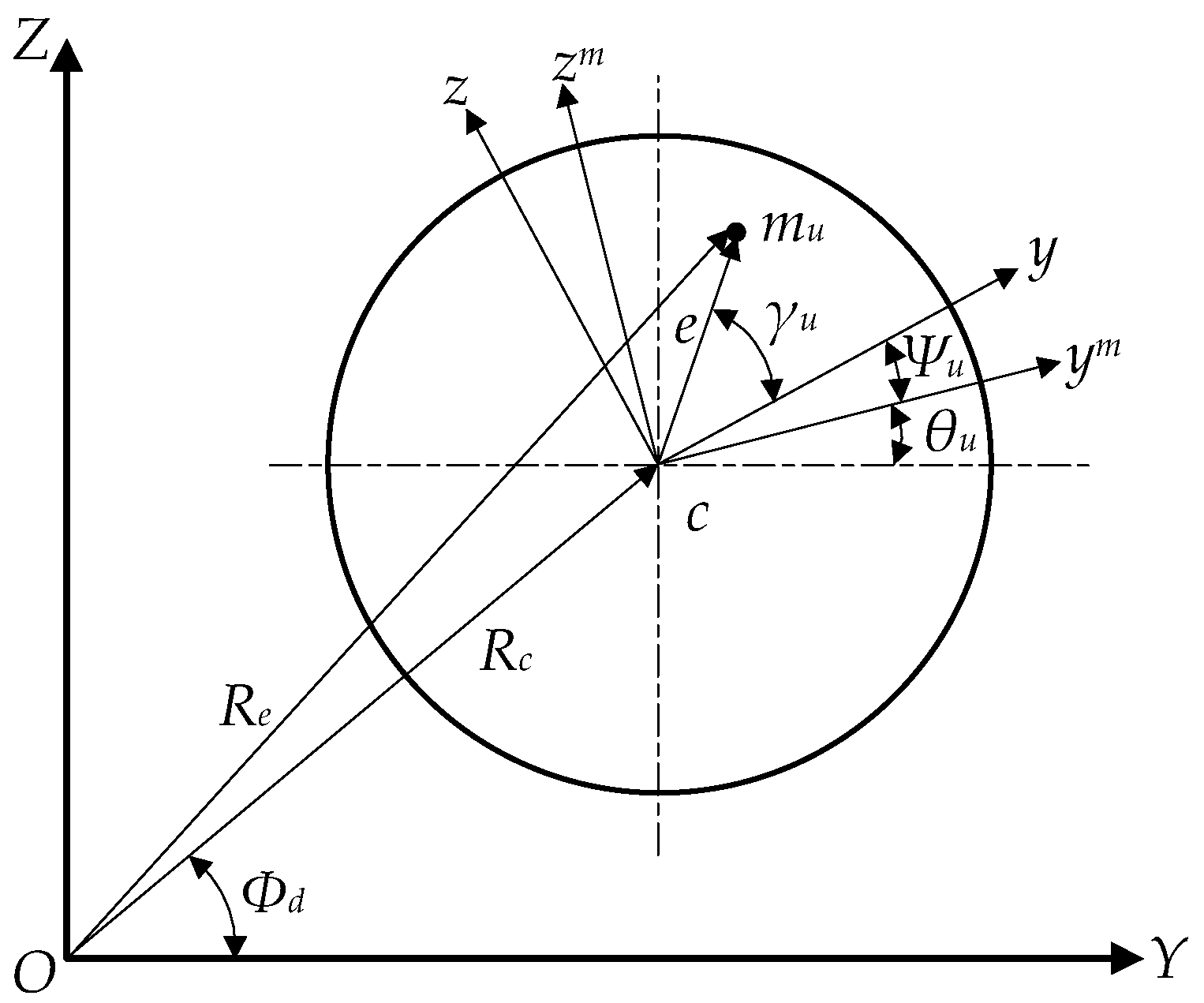
In the process of helical gear meshing, due to the existence of eccentric mass, the bending, torsion and axial deformation in the system show a high degree of coupling characteristics. The eccentric mass element not only changes the natural vibration mode of the system but also causes a complex asymmetric vibration response related to time, which is particularly significant under high-speed operation conditions. To simplify the calculations, the disk tilt angle is assumed to be 0. The coordinate system and deformation configuration of the eccentric mass element are shown in Figure 1.

The bending–torsion coupling dynamic model of the rotor–bearing with eccentric mass is shown in references [25,26]. In this paper, each node is considered to have 6 degrees of freedom, the eccentric mass is regarded as an independent element, and the gear is regarded as a disc element, considering its mass and moment of inertia. As shown in Figure 1, Y-Z is a fixed inertial reference coordinate system; y^m-z^m is a coordinate system accompanied by the rotation of the disc; y-z is the coordinate system accompanied by the torsion of the disc, and it is also the plane where the eccentric mass is located. θ_u = Ωt is the angular displacement of the disk relative to the fixed inertial reference coordinate system at any time. ψ_u is the torsion angle of the disk relative to the y^m-z^m coordinate at any time. m_u is an eccentric mass. e is the distance between the eccentric mass and the center of the disk. e_y and e_z are components of vector e = [e_y e_z]^T. γ_u and e represent the position of the eccentric mass on the disk, and R_c and ϕ_d represent the center position of the disk, where c denotes the center of the disk. Ignoring the influence of disk tilt, the kinetic energy of the eccentric disk-shaft system can be expressed as [27]

$$T_d^u={\displaystyle \frac{1}{2}}{m}_d({\dot{y}}_d^2+{\dot{z}}_d^2)+{\displaystyle \frac{1}{2}}{J}_d{({\dot{\theta }}_u+{\dot{\psi }}_u)}^2 +{\displaystyle \frac{1}{2}}{J}_p{\dot{\theta }}_u^2+{\displaystyle \frac{1}{2}}{\displaystyle \sum _{i=1}^n{m}_u{\dot{\mathit{R}}}_e^T{\dot{\mathit{R}}}_e}$$

(11)

The eccentric mass is regarded as an independent element, and the last item of Equation (11) is extracted, which is the kinetic energy of a single dynamic eccentric mass:

$$T_u={\displaystyle \frac{1}{2}}{m}_u{\dot{\mathit{R}}}_e^T{\dot{\mathit{R}}}_e$$

(12)

Assuming that the torsional vibration angle is very small, that is, cosψ_u ≈ 1, sinψ_u ≈ ψ_u, the global position vector R_e of the eccentric mass m_u under the inertial reference coordinate system can be written as

$$\begin{array}{l}{\mathit{R}}_e=\left\{\begin{array}{c}{y}_u\\ z_u\end{array}\right\}+\left[\begin{array}{cc}\cos {\theta }_u& -\sin {\theta }_u\\ \sin {\theta }_u& \cos {\theta }_u\end{array}\right]\left[\begin{array}{cc}\cos {\psi }_u& -\sin {\psi }_u\\ \sin {\psi }_u& \cos {\psi }_u\end{array}\right]\left[\begin{array}{c}{e}_y\\ e_z\end{array}\right]\\ \approx \left\{\begin{array}{c}{y}_u\\ z_u\end{array}\right\}+\left[\begin{array}{cc}\cos {\theta }_u& -\sin {\theta }_u\\ \sin {\theta }_u& \cos {\theta }_u\end{array}\right]\left[\begin{array}{cc}1& -{\psi }_u\\ {\psi }_u& 1\end{array}\right]\left[\begin{array}{c}{e}_y\\ e_z\end{array}\right]\\ =\left\{\begin{array}{c}{y}_u+(e_y-{\psi }_u{e}_z)\cos {\theta }_u-({\psi }_u{e}_y+e_z)\sin {\psi }_u\\ z_u+(e_y-{\psi }_u{e}_z)\sin {\psi }_u-({\psi }_u{e}_y+e_z)\cos {\theta }_u\end{array}\right\}\end{array}$$

(13)

where y_u and z_u are the horizontal displacement and vertical displacement of the eccentric mass at any time in the y-z coordinate. Derivation of the global position vector R_e yields:

$${\dot{\mathit{R}}}_e=\left\{\begin{array}{c}\begin{array}{l}{\dot{y}}_u-{\dot{\theta }}_u{e}_y\sin {\theta }_u-{\dot{\psi }}_u{e}_z\cos {\theta }_u+{\dot{\theta }}_u{\psi }_u{e}_z\sin {\theta }_u\\ -{\dot{\psi }}_u{e}_y\sin {\theta }_u-{\dot{\theta }}_u{\psi }_u{e}_y\cos {\theta }_u-{\dot{\theta }}_u{e}_z\cos {\theta }_u\end{array}\\ \begin{array}{l}{\dot{z}}_u+{\dot{\theta }}_u{e}_y\cos {\theta }_u-{\dot{\psi }}_u{e}_z\sin {\theta }_u-{\dot{\theta }}_u{\psi }_u{e}_z\cos {\theta }_u\\ +{\dot{\psi }}_u{e}_y\cos {\theta }_u-{\dot{\theta }}_u{\psi }_u{e}_y\sin {\theta }_u-{\dot{\theta }}_u{e}_z\sin {\theta }_u\end{array}\end{array}\right\}$$

(14)

Substituting Equation (14) into Equation (12), the kinetic energy equation of dynamic eccentric mass is obtained:

$$\begin{array}{c}{T}_u=m_u({\dot{y}}_u^2+{\dot{z}}_u^2)/2+m_u[{({\dot{\psi }}_{u}e)}^2+{({\dot{\theta }}_{u}e)}^2+{({\dot{\theta }}_u{\dot{\psi }}_{u}e)}^2]/2 +m_u{\dot{\theta }}_u{\dot{\psi }}_u{e}^2 +m_u{\dot{\psi }}_u{\dot{z}}_u{A}_2\\ -m_u{\dot{\psi }}_u{\dot{y}}_u{A}_1-m_u{\dot{\theta }}_u{\dot{z}}_u{\psi }_u{A}_1 +m_u{\dot{\theta }}_u{\dot{z}}_u{A}_2 -m_u{\dot{\theta }}_u{\dot{y}}_u{A}_1-m_u{\dot{\theta }}_u{\dot{y}}_u{\psi }_u{A}_2\end{array}$$

(15)

where e² = $e_y^2$ + $e_z^2$, A₁ = e_ysinθ_u − e_zcosθ_u, A₂ = e_ycosθ_u − e_zsinθ_u.

$${\displaystyle \frac{\partial T_u}{\partial y_u}}={\displaystyle \frac{\partial T_u}{\partial z_u}}=0$$

(16)

$${\displaystyle \frac{\partial T_u}{\partial {\dot{y}}_u}}=m_u{\dot{y}}_u-m_u{\psi }_u{A}_1-m_u{\dot{\theta }}_u{A}_1-m_u{\dot{\theta }}_u{\psi }_u{A}_2$$

(17)

$${\displaystyle \frac{d}{dt}}\left({\displaystyle \frac{\partial T_u}{\partial {\dot{y}}_u}}\right)=m_u{\ddot{y}}_u-m_u{\dot{\psi }}_u{A}_1-m_u{\dot{\psi }}_u{\dot{\theta }}_u{A}_2-m_u{\ddot{\theta }}_u{A}_1-m_u{\dot{\theta }}_u^2{A}_2-m_u{\ddot{\theta }}_u{\psi }_u{A}_2+m_u{\dot{\theta }}_u^2{\psi }_u{A}_1-m_u{\dot{\psi }}_u{\dot{\theta }}_u{A}_2$$

(18)

$${\displaystyle \frac{\partial T_u}{\partial {\dot{z}}_u}}=m_u{\dot{z}}_u+m_u{\dot{\psi }}_u{A}_2+m_u{\dot{\theta }}_u{A}_2-m_u{\dot{\theta }}_u{\psi }_u{A}_1$$

(19)

$${\displaystyle \frac{d}{dt}}\left({\displaystyle \frac{\partial T_u}{\partial {\dot{z}}_u}}\right)=m_u{\ddot{z}}_u+m_u{\ddot{\psi }}_u{A}_2-m_u{\dot{\psi }}_u{\dot{\theta }}_u{A}_1+m_u{\ddot{\theta }}_u{A}_2-m_u{\dot{\theta }}_u^2{A}_1-m_u{\ddot{\theta }}_u{\psi }_u{A}_1-m_u{\dot{\theta }}_u^2{\psi }_u{A}_2-m_u{\dot{\psi }}_u{\dot{\theta }}_u{A}_1$$

(20)

$${\displaystyle \frac{\partial T_u}{\partial {\psi }_u}}=m_u{e}^2{\dot{\theta }}_u^2{\psi }_u-m_u{\dot{\theta }}_u{\dot{z}}_u{A}_1-m_u{\dot{\theta }}_u{\dot{y}}_u{A}_2$$

(21)

$${\displaystyle \frac{\partial T_u}{\partial {\dot{\psi }}_u}}=m_u{e}^2{\dot{\psi }}_u+m_u{e}^2{\dot{\theta }}_u+m_u{\dot{z}}_u{A}_2-m_u{\dot{y}}_u{A}_1$$

(22)

$${\displaystyle \frac{d}{dt}}\left({\displaystyle \frac{\partial T_u}{\partial {\dot{\psi }}_u}}\right)=m_u{e}^2{\ddot{\psi }}_u+m_u{e}^2{\ddot{\theta }}_u+m_u{\ddot{z}}_u{A}_2-m_u{\dot{z}}_u{\dot{\theta }}_u{A}_1 -m_u{\ddot{y}}_u{A}_1+m_u{\dot{y}}_u{\dot{\theta }}_u{A}_2$$

(23)

Applying the Lagrangian equation and assuming that there is no initial phase angle, ignoring the higher-order terms of θ_u, they are written in the form of a matrix.

Lagrangian equation:

$${\displaystyle \frac{\partial }{\partial t}}({\displaystyle \frac{\partial T_u}{\partial {\dot{\mathit{q}}}_u}})-{\displaystyle \frac{\partial T_u}{\partial {\mathit{q}}_u}}={\mathit{F}}_{q_u}$$

(24)

The dynamic equation of the dynamic eccentric mass can be written as

$${\mathit{M}}_u(t){\ddot{q}}_u+{\mathit{C}}_u(t){\dot{q}}_u+{\mathit{K}}_u(t){\mathit{q}}_u={\mathit{F}}_u(t)$$

(25)

$${\mathit{M}}_u=\left[\begin{array}{cccccc}{m}_1^u& 0& 0& 0& 0& 0\\ 0& m_1^u& 0& -m_1^u{A}_1& 0& 0\\ 0& 0& m_1^u& m_1^u{A}_2& 0& 0\\ 0& -m_1^u{A}_1& m_1^u{A}_2& m_1^u{e}^2& 0& 0\\ 0& 0& 0& 0& 0& 0\\ 0& 0& 0& 0& 0& 0\end{array}\right]$$

(26)

$${\mathit{K}}_u=\left[\begin{array}{cccccc}0& 0& 0& 0& 0& 0\\ 0& 0& 0& m_1^u{\dot{\theta }}_d^2{A}_1& 0& 0\\ 0& 0& 0& -m_1^u{\dot{\theta }}_d^2{A}_2& 0& 0\\ 0& 0& 0& -m_1^u{e}^2{\dot{\theta }}_d^2& 0& 0\\ 0& 0& 0& 0& 0& 0\\ 0& 0& 0& 0& 0& 0\end{array}\right]$$

(27)

$${\mathit{C}}_u=\left[\begin{array}{cccccc}0& 0& 0& 0& 0& 0\\ 0& 0& 0& -2m_1^u\dot{\theta }{A}_2& 0& 0\\ 0& 0& 0& -2m_1^u\dot{\theta }{A}_1& 0& 0\\ 0& 0& 0& 0& 0& 0\\ 0& 0& 0& 0& 0& 0\\ 0& 0& 0& 0& 0& 0\end{array}\right]$$

(28)

$${\mathit{F}}_u=\left[\begin{array}{c}{m}_{u}e{\mathsf{\Omega }}^2\cos \theta \\ m_{u}e{\mathsf{\Omega }}^2\sin \theta \\ 0\\ 0\\ 0\\ 0\end{array}\right]$$

(29)

$${\mathit{q}}_{\mathit{u}}={\left[\begin{array}{cccccc}{x}_u& y_u& z_u& {\theta }_{xu}& {\theta }_{yu}& {\theta }_{zu}\end{array}\right]}^T$$

(30)

Equation (30) is the displacement vector of the eccentric disk, x is the axial direction, and y and z are transverse directions. K_u and C_u are asymmetric matrices, resulting in bending–torsion–axial coupling and time-dependent behavior.

2.3. Bearing Elements

In the high-speed gear transmission, the bearing plays a supporting role. This paper employs rolling bearings for support. In this work, four spring coefficients (k_yy, k_yz, k_zy, and k_zz) and four damping coefficients (c_yy, c_yz, c_zy, and c_zz) are used to simulate the bearing element. Within this model, it is assumed that the force on each bearing follows the following form of control equation:

$$\left[\begin{array}{cc}{c}_{yy}& c_{yz}\\ c_{zy}& c_{zz}\end{array}\right]{\dot{q}}_b+\left[\begin{array}{cc}{k}_{yy}& k_{yz}\\ k_{zy}& k_{zz}\end{array}\right]{\mathit{q}}_b={\mathit{F}}_b$$

(31)

where q_b is the displacement vector of the bearing, c_ij and k_ij are the damping coefficients and stiffness coefficients of the bearing, respectively; F_b is the vector of bearing force. The bearing element matrix is combined into the overall dynamic equation.

2.4. Global Dynamic Equation

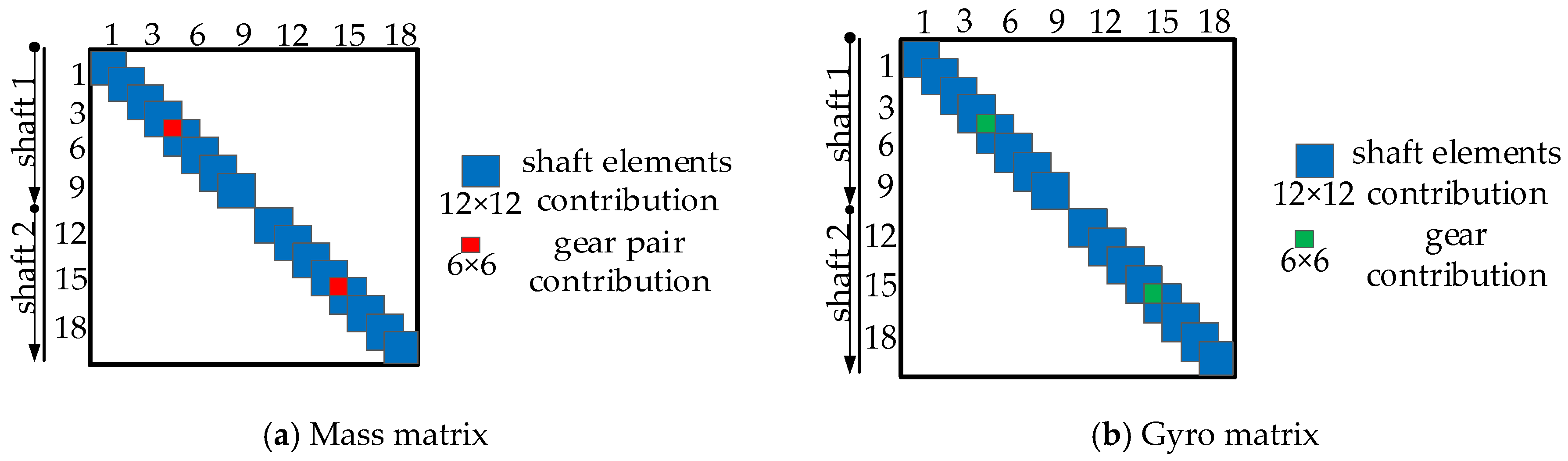
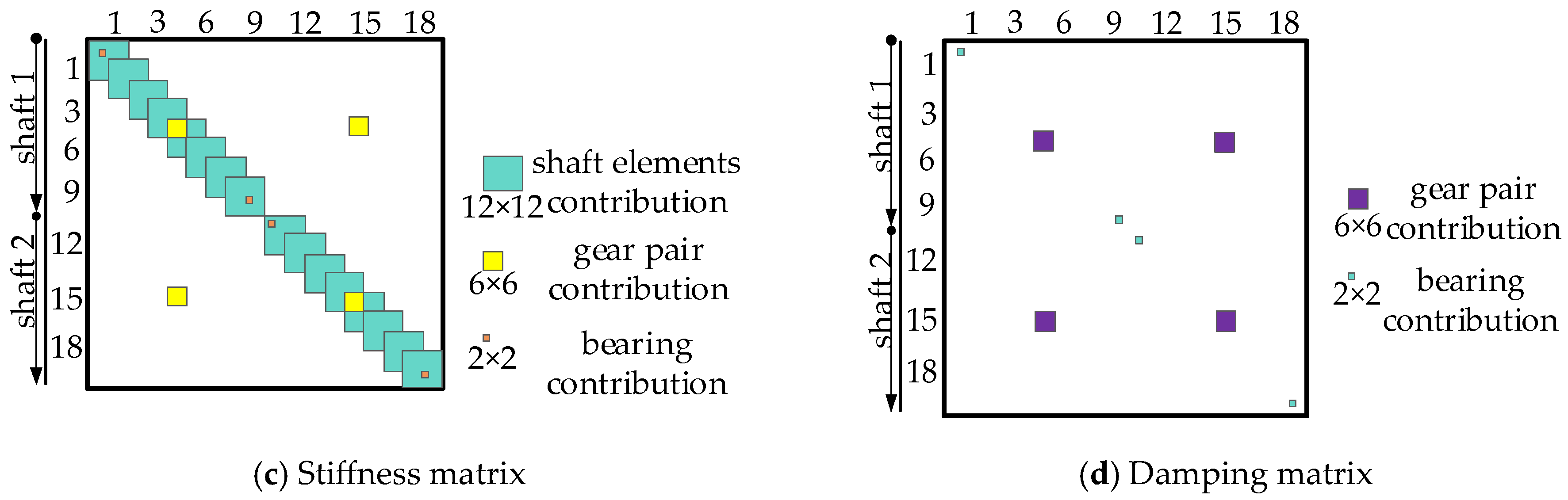
The assembly method of the shaft–helical gear–bearing system is shown in Figure 2, in which the mass matrix is M = (M_s, M_c, M_b, M_u), the gyroscopic matrix is G = (G_s, G_c), the stiffness matrix is K = (K_s, K_c, K_b, K_u), and the damping matrix is C = (C_b, C_u). M_s, G_s, and K_s are the element matrices of the shaft; K_c is the gear meshing stiffness matrix; and C_b and K_b are the damping and stiffness matrices of the bearing.

Figure 2 illustrates the assembly of the shaft–helical gear–bearing system. Figure 2a shows the assembly method of the mass matrix, where the blue block represents a 12 × 12 shaft element matrix, and the red block represents a 6 × 6 gear element matrix. Figure 2b depicts the assembly method of the gyroscopic matrix, where the blue block represents a 12 × 12 shaft element matrix and the green block represents a 6 × 6 gear element matrix. Figure 2c shows the assembly method of the stiffness matrix, with the light blue block representing a 12 × 12 shaft element matrix, the yellow block representing a 6 × 6 gear element matrix, and the orange block indicating a 2 × 2 bearing element matrix. Figure 2d illustrates the assembly method of the damping matrix, with the purple block representing a 6 × 6 gear element matrix and the green block representing a 2 × 2 bearing element matrix.

According to the finite element theory, the shaft element, bearing element, gear meshing element and eccentric mass element are combined together [28] to form a system dynamics model:

$$(\mathit{M}+{\mathit{M}}_u(t))\ddot{\mathit{q}}+(\mathsf{\Omega }\mathit{G}+\mathit{C}+{\mathit{C}}_u(t))\dot{\mathit{q}}+(\mathit{K}+{\mathit{K}}_u(t))\mathit{q}=\mathit{F}+{\mathit{F}}_u(t)$$

(32)

where the mass matrix (M + M_u(t)), damping matrix (ΩG + C+ C_u(t)) and stiffness matrix (K + K_u(t)) vary at each time step. The matrix of dynamic eccentricity led to the time-varying characteristic of the coupled lateral–torsional vibration. Hence, the coupled system becomes a parameter excitation system. (F + F_u(t)) is the generalized force vector of the system, including the unbalanced excitation force, external periodic excitation force, and moment.

Considering Rayleigh structural damping,

$$C_s={\alpha }_1\mathit{M}+{\alpha }_2\mathit{K}$$

(33)

where α₁ and α₂ are proportional coefficients:

$$\left\{\begin{array}{c}{\alpha }_1\\ {\alpha }_2\end{array}\right\}={\displaystyle \frac{2\lambda }{{\omega }_i+{\omega }_j}}\left\{\begin{array}{c}{\omega }_i{\omega }_j\\ 1\end{array}\right\}$$

(34)

where ω_i and ω_j are the frequency bands of interest in the modal analysis of the system. By comprehensively considering the frequency components of the external load and the dynamic characteristics of the structure, λ is the damping ratio, which is generally obtained by a vibration test or simulation.

3. Time-Varying Meshing Stiffness Model of Helical Gear

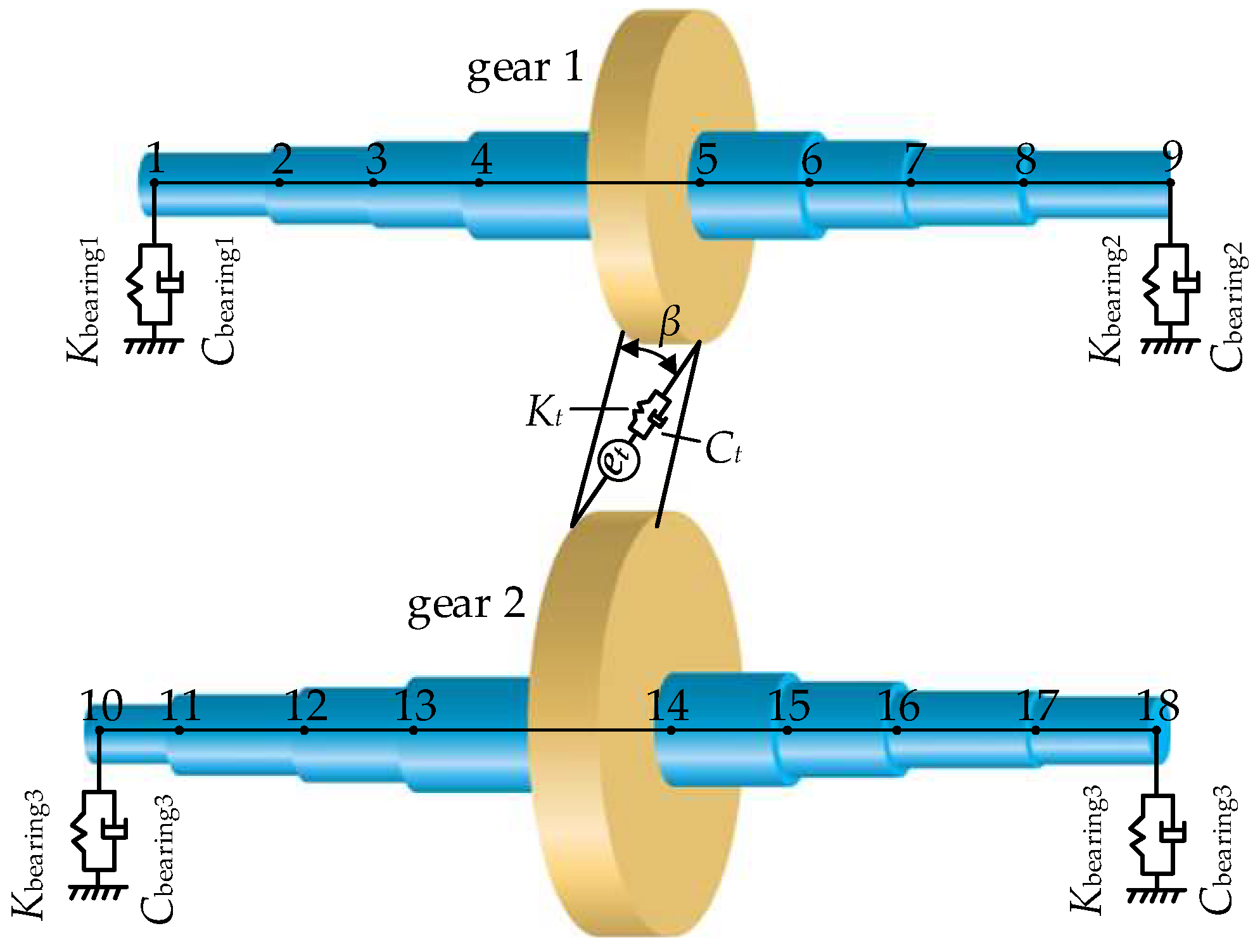
In the literature [11,12,13,14], the mathematical model of helical gear meshing is regarded as a lumped mass element, and its time-varying stiffness and time-varying damping are derived in detail. The stiffness and damping of each meshing position are 12 × 12. It is assumed that a pair of helical gears is transmitted. According to the aforementioned rotor dynamics model, the time-varying matrix can be added to the two parallel shafts for power transmission. The power transmission model of the helical gear–rotor–bearing system is shown in Figure 3. Meanwhile, gear 1 is the active gear, and gear 2 is the driven gear. Each gear shaft is discretely modeled through nine finite element nodes, and support stiffness elements K_b1, K_b2, K_b3, and K_b4 and corresponding support damping elements C_b1, C_b2, C_b3, and C_b4 are set at both ends to simulate the bearing support characteristics. The meshing relationship between gears is characterized by time-varying meshing stiffness K_t and meshing damping C_t to reflect the periodic change characteristics of meshing stiffness during gear rotation.

4. Parametric Excitation Analysis of Eccentricity and Meshing Time-Varying Stiffness

Because the meshing stiffness and eccentricity matrix are related to time, the system belongs to the category of parametric excitation systems, and the transient dynamic analysis of the system is carried out. Eccentric mass of driving wheel $m_1^u = m_2^u$ = 0.2 kg, eccentric distance e₁ = e₂ = 0.02 m. The size of the shaft is as follows: each shaft length is 1 m, divided into 8 elements; the radius is 0.015 m; the elastic modulus is 2.1 × 10¹¹ Pa; the Poisson’s ratio is 0.3; and the density is 7850 kg/m³. The shaft is made of 17CrNiMo6 steel with a yield strength of 835 MPa. Therefore, the two shafts have 16 Timoshenko beam elements, a total of 18 nodes, and four bearings are located at 1, 9, 10, and 18 nodes, respectively. The two gears are numbered at the nodes of 5 and 14, respectively. Bearing stiffness k_yy = 2.0 × 10⁸ N/m, k_yz = 0, k_zy = 0, k_zz = 4.0 × 10⁸ N/m, without considering the bearing damping. The parameters of gears 1 and 2 are shown in

Table 1. Gear 1 parameters (right-hand thread).

Normal Module	Tooth Number	Helix Angle	Normal Pressure Angle	Tooth Height Coefficient	Bottom Clearance Coefficient
3 mm	17	20°	20°	1	0.25

and

Table 2. Gear 2 parameters (left-hand thread).

Normal Module	Tooth Number	Helix Angle	Normal Pressure Angle	Tooth Height Coefficient	Bottom Clearance Coefficient
3 mm	60	20°	20°	1	0.25

.

The mass of gear 1 and gear 2 is 9.20 kg and 46.20 kg, respectively; the diameter moment of inertia is 0.03 kg‧m² and 0.50 kg‧m², respectively; and the polar moment of inertia is 0.06 kg‧m² and 0.98 kg‧m², respectively. The drive motor has an output power of 132 kW, corresponding to the input torque applied to the driving shaft, which is approximately 126 Nm, and the speed is 10,000 r/min.

The displacement response is calculated by the integration method Newmark β using a MATLAB R2024a routine. The mathematical calculation procedure is as follows:

1. Initial calculation:

(1) Compute matrices M, K and (ΩG + C);

(2) Compute matrices M_u(t), K_u(t), C_u(t) and F_u(t);

(3) Initial displacement, velocity and acceleration: ${\mathit{u}}_0$, ${\dot{u}}_0$ and ${\ddot{\mathit{u}}}_0$;

(4) Choose integration time step Δt, γ, and β and calculate the integration constants:

$${\alpha }_0={\displaystyle \frac{1}{\gamma \Delta t^2}},{\alpha }_1={\displaystyle \frac{\beta }{\gamma \Delta t}},{\alpha }_2={\displaystyle \frac{1}{\gamma \Delta t}},{\alpha }_3={\displaystyle \frac{1}{2\gamma }}-1,{\alpha }_4={\displaystyle \frac{\beta }{\gamma }}-1,{\alpha }_5={\displaystyle \frac{\Delta t}{2}}({\displaystyle \frac{\beta }{\gamma }}-2),{\alpha }_6=\Delta t(1-\beta ),{\alpha }_7=\beta \Delta t$$

(35)

(5) Compute the effective stiffness matrix

$$\overline{\mathit{K}}=(K+{\mathit{K}}_u(t))+{\alpha }_0(M+{\mathit{M}}_u(t))+{\alpha }_1(\mathsf{\Omega }G+C+{\mathit{C}}_u(t))$$

(36)

2. For each time step:

(1) Compute the effective force vector at time $t+\Delta t$

$$\begin{array}{c}{(\overline{F}+{\overline{F}}_u(t))}_{t+\Delta t}={(F+F_u(t))}_{t+\Delta t}+(\mathit{M}+M_u(t))({\alpha }_0{q}_t+{\alpha }_2{\dot{q}}_t+{\alpha }_3{\ddot{q}}_t)\\ +(\mathsf{\Omega }G+\mathit{C}+C_u(t))({\alpha }_1{q}_t+{\alpha }_4{\dot{q}}_t+{\alpha }_5{\ddot{q}}_t)\end{array}$$

(37)

(2) Find the displacement at time

$$\overline{\mathit{K}}{\mathit{q}}_{t+\Delta t}={(\overline{F}+{\overline{\mathit{F}}}_u(t))}_{t+\Delta t}$$

(38)

(3) Find the acceleration and velocity at time

$${\ddot{\mathit{q}}}_{t+\Delta t}={\alpha }_0({\mathit{q}}_{t+\Delta t}-{\mathit{q}}_t)-{\alpha }_2{\dot{\mathit{q}}}_t-{\alpha }_3{\ddot{\mathit{q}}}_t$$

(39)

$${\dot{\mathit{q}}}_{t+\Delta t}={\dot{\mathit{q}}}_t+{\alpha }_6{\ddot{\mathit{q}}}_t+{\alpha }_7{\ddot{\mathit{q}}}_{t+\Delta t}$$

(40)

3. Repeat step 2 for the next time step.

4. Calculate the dynamic stress by the displacement response:

$$\mathit{\sigma }=\mathit{D}\mathit{B}\mathit{q}$$

(41)

where D = diag(E E E G κG κG) is the elastic matrix corresponding to the material, E is the elastic modulus, G is the shear modulus, and κ = 0.886 is the transverse shear form factor.

$$\mathit{B}={\left[\begin{array}{c}{\displaystyle \frac{\partial {\mathit{N}}_x}{\partial x}}, {\displaystyle \frac{\partial {\mathit{N}}_y}{\partial x}}, {\displaystyle \frac{\partial {\mathit{N}}_z}{\partial x}}, {\displaystyle \frac{\partial {\mathit{N}}_{\theta x}}{\partial x}}, {\displaystyle \frac{\partial {\mathit{N}}_y}{\partial x}}-{\mathit{N}}_{\theta z}, {\displaystyle \frac{\partial {\mathit{N}}_z}{\partial x}}-{\mathit{N}}_{\theta y}\end{array}\right]}^T$$

(42)

N = [N_x N_y N_z N_θx N_θy N_θz]^T is the shape function of the Timoshenko beam.

The finite element modeling of the gear meshing structure shown in Figure 3 is carried out, and the dynamic numerical calculation is carried out by using the Newmark β method to obtain the displacement response on the shaft, as shown in Figure 4.

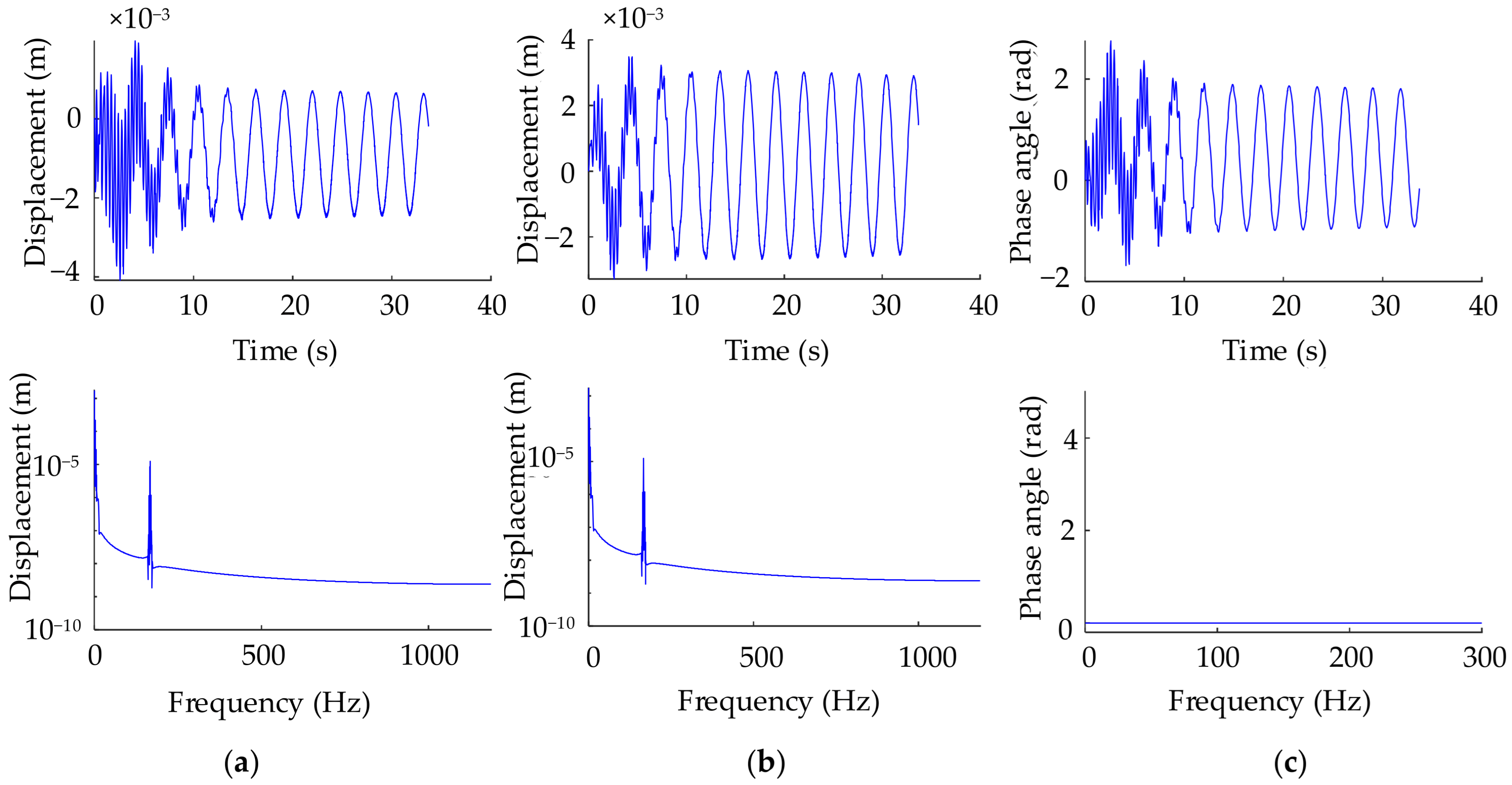
Figure 4a,b present the vibration responses of the shaft with a time-varying meshing stiffness matrix in the y-z directions. Figure 4c presents the torsional vibration response along the x-axis, as well as the evolution of the shaft’s axial orbit over time. From the bending vibration response shown in Figure 4a, it can be observed that the time-varying stiffness matrix influences not only the degrees of freedom along the main diagonal but also exerts a significant effect on the coupled degrees of freedom.

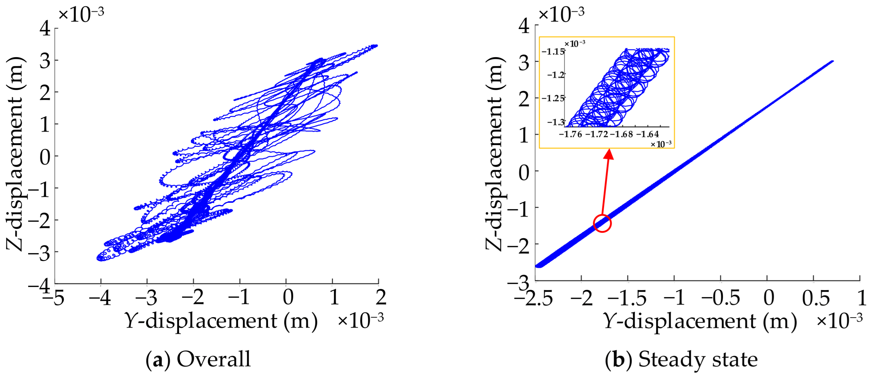
The transient shaft orbit in the Y-Z plane is shown in Figure 5. Figure 5a presents the overall transient orbit of the shaft in the Y-Z plane under the influence of time-varying mesh stiffness. The orbit exhibits pronounced nonlinear and coupled dynamic characteristics, indicating significant coupling effects between translational degrees of freedom. Figure 5b provides a magnified view of a local region from Figure 5a, revealing detailed features of the orbital structure. An additional inset in Figure 5b further enlarges the orbit enclosed by the circular marker. It can be observed that, after initial transients, the shaft orbit in the Y-Z plane gradually converges to a more regular pattern, suggesting that the system response transitions into a steady-state regime.

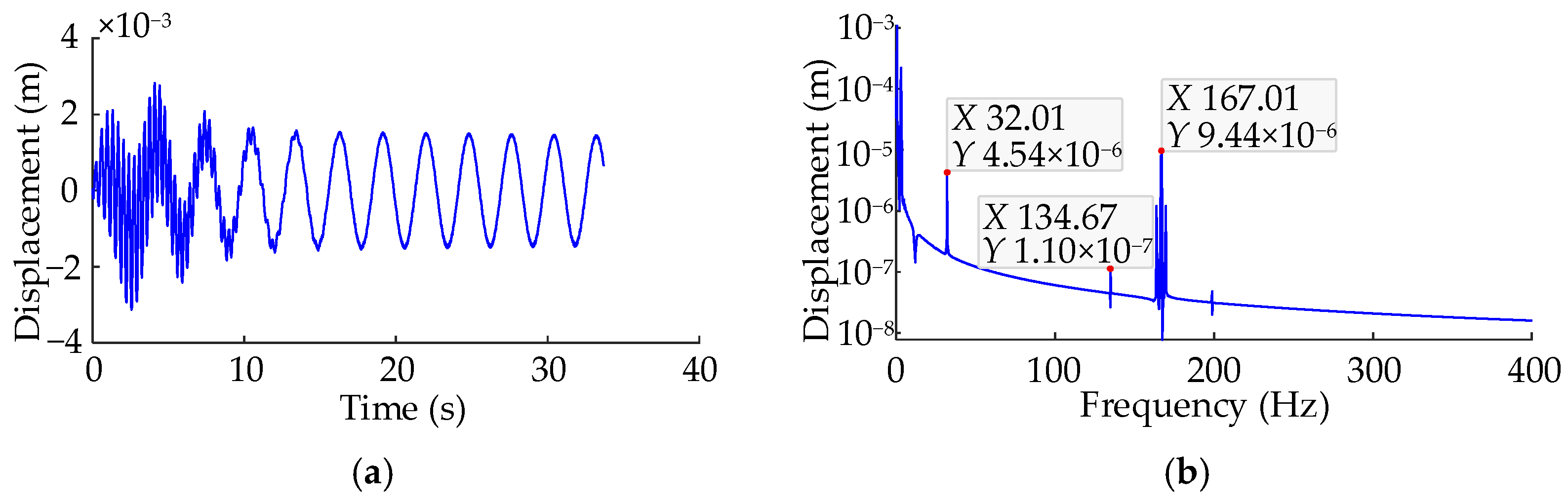
To examine different working conditions, inputting an external torsional excitation to the motor drive produces a bending vibration response with a frequency that is the difference between the bending natural frequency and the torsional excitation frequency. Specifically, a torsional excitation of 32 Hz applied to the input shaft produces a coupled bending vibration response of 134.9998 (=167.014 − 32.0142) Hz, which is approximately equal to the peak value of 134.673 Hz in Figure 6.

The result indicates that a coupled bending and torsional vibration phenomenon is generated under the influence of the mechanically eccentric mass. In contrast, since the input is a constant torque, Figure 4a does not produce a coupled bending vibration response.

For different materials, it is not appropriate to use the same yield criterion. The Von Mises criterion is not universal but only a special case. Using the same strength criterion to evaluate materials with different material properties will cause certain errors. The fourth strength theory of materials considers the influence of intermediate principal stress but does not consider the influence of the difference between the tensile and compressive strength of materials. The unified strength theory proposed by Yu [29] is suitable for the analysis of complex stress states. For the Timoshenko beam element, after obtaining the displacement response of the nodes at both ends of an element, the stress of a specific point on a section of the element is obtained by the element type function and the strain–stress relationship, including two transverse normal stresses, one axial normal stress, and one axial torsional shear stress. A complex stress state can be represented by a 3 × 3 stress tensor:

$${\mathit{\sigma }}_{ij}=\left[\begin{array}{ccc}{\sigma }_x& {\tau }_{xy}& {\tau }_{xz}\\ {\tau }_{yx}& {\sigma }_y& {\tau }_{yz}\\ {\tau }_{zx}& {\tau }_{zy}& {\sigma }_z\end{array}\right]$$

(43)

The characteristic equation of the symmetric stress matrix is

$${\sigma }^3-I_1{\sigma }^2+I_2\sigma -I_3=0$$

(44)

where

$$I_1={\sigma }_x+{\sigma }_y+{\sigma }_z$$

(45)

$$I_2={\sigma }_x{\sigma }_y+{\sigma }_y{\sigma }_z+{\sigma }_z{\sigma }_x-{\tau }_{xy}^2-{\tau }_{yz}^2-{\tau }_{zx}^2$$

(46)

$$I_3={\sigma }_x{\sigma }_y{\sigma }_z+2{\tau }_{xy}{\tau }_{yz}{\tau }_{zx}-{\sigma }_x{\tau }_{yz}^2-{\sigma }_y{\tau }_{zx}^2-{\sigma }_z{\tau }_{xy}^2$$

(47)

The eigenvalues of the characteristic equation are arranged into three principal stresses, σ₁, σ₂, σ₃, and the eigenvectors corresponding to the eigenvalues represent the direction of the principal stress.

When the two large shear stresses acting on the twin-shear element and the normal stress combination on the surface reach a certain limit value, the material will yield, that is, the unified yield criterion of metal materials under complex stress states. Any complex stress state can be transformed into a twin-shear stress state, and the twin-shear element can be obtained by changing the shape of the element.

The twin-shear stress yield criterion can better reflect the influence of the intermediate principal stress. For example, the intermediate principal stress can improve the yield limit of the material. The twin-shear stress yield criterion holds that when the sum of the absolute values of the two large principal shear stresses reaches a certain limit value C, the material begins to yield. The expression of the yield criterion is as follows:

$$\left|{\tau }_{13}\right|+\left|{\tau }_{12}\right|={\sigma }_1-({\sigma }_2+{\sigma }_3)/2={\sigma }_{\mathrm{s}},\left|{\tau }_{12}\right|>\left|{\tau }_{23}\right|$$

(48)

$$\left|{\tau }_{13}\right|+\left|{\tau }_{23}\right|=({\sigma }_1+{\sigma }_2)/2-{\sigma }_3={\sigma }_{\mathrm{s}},\left|{\tau }_{12}\right|<\left|{\tau }_{23}\right|$$

(49)

For materials with SD effect (unequal tensile and compressive strength), such as high-strength steel, the material yield criterion considering the influence of intermediate principal stress and unequal tensile and compressive strength is

$${\tau }_{13}+b{\tau }_{12}+\beta ({\sigma }_{13}+b{\sigma }_{12})=C,({\tau }_{12}+\beta {\sigma }_{12})\ge ({\tau }_{23}+\beta {\sigma }_{23})$$

(50)

$${\tau }_{13}+b{\tau }_{23}+\beta ({\sigma }_{13}+b{\sigma }_{23})=C,({\tau }_{12}+\beta {\sigma }_{12})\le ({\tau }_{23}+\beta {\sigma }_{23})$$

(51)

$$C={\displaystyle \frac{2{\sigma }_{ts}}{1+\alpha }}$$

(52)

In the yield criterion, b is the selection parameter, which represents the influence degree of intermediate principal stress. σ_ts and σ_cs are the tensile and compressive strength limits, respectively, which can be directly determined by the three-dimensional stress test.

$$\beta ={\displaystyle \frac{{\sigma }_{cs}-{\sigma }_{ts}}{{\sigma }_{cs}+{\sigma }_{ts}}}={\displaystyle \frac{1-\alpha }{1+\alpha }}$$

(53)

Equation (53) represents the effect of different tensile and compressive strengths. α = σ_ts/σ_cs, when σ = 1 and b = 0.577, the unified strength theory degenerates to the Von Mises criterion. When α = 1 and b = 1, the unified strength theory degenerates into the twin-shear yield criterion.

For the stressed object, the first two larger principal shear stresses, σ₁ and σ_2, have a greater impact. The sum of two larger principal shear stresses at a certain point is obtained, that is, the twin-shear stress:

$${\tau }_{13}={\displaystyle \frac{{\sigma }_1-{\sigma }_3}{2}},{\tau }_{12}={\displaystyle \frac{{\sigma }_1-{\sigma }_2}{2}},{\tau }_{23}={\displaystyle \frac{{\sigma }_2-{\sigma }_3}{2}}$$

(54)

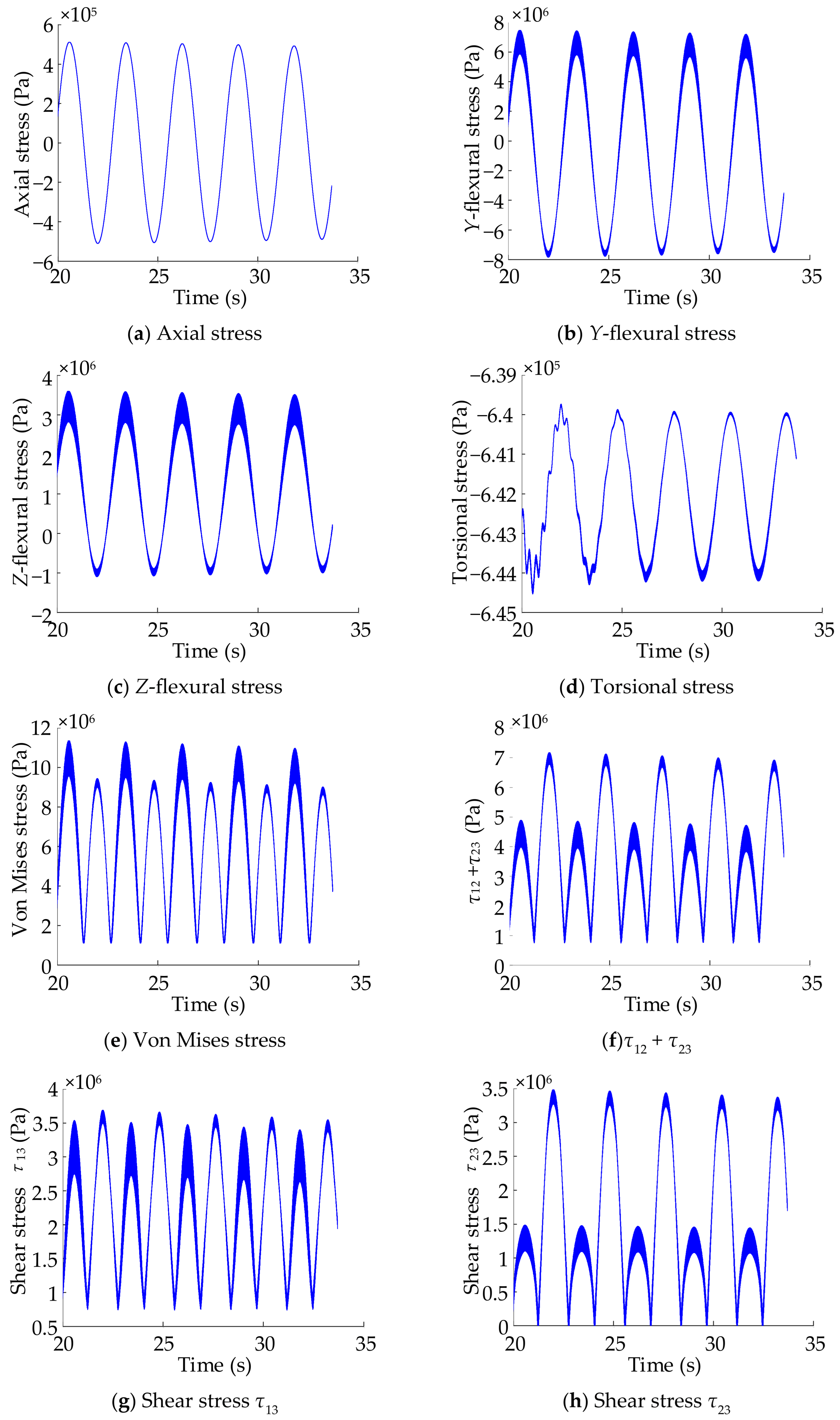
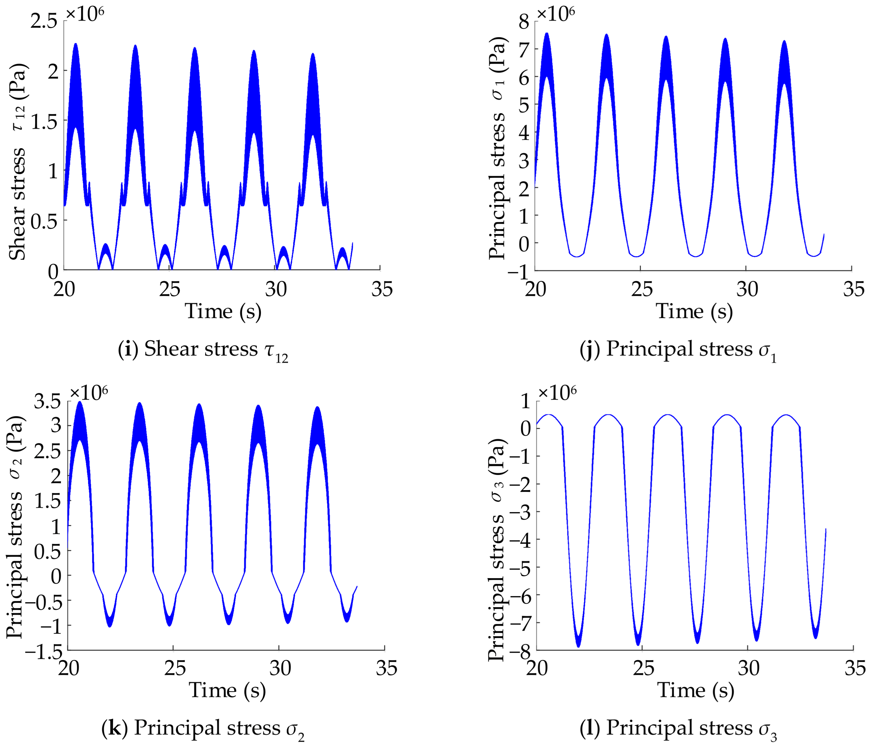
According to the geometric conditions and stress conditions, the relationship between displacement and strain can be derived through the type function, while the stress is obtained through the stress matrix. Since the system enters a stable state starting from 20 s, the presented results are from after 20 s. The results are shown in Figure 7. The deformation of each degree of freedom on the axis will lead to dynamic stress.

Twin-shear stress is more realistic, which is confirmed by three-dimensional experiments. Figure 7e,f indicates that the Von Mises equivalent stress and the twin-shear stress are less than the yield strength of the gear material, and the Von Mises equivalent stress is greater than the twin-shear stress, which conforms to the unified strength theory; that is, when the equivalent stress is used to judge that the vibration intensity reaches the yield limit, but the twin-shear stress has not yet reached it, the load can continue to be applied to the object. There is a certain margin, which is beneficial to the utilization rate of the material and is suitable for lightweight design.

5. Conclusions

In this study, the dynamic response of the helical gear transmission system is deduced and analyzed based on time-varying stiffness, and the influence of time-varying stiffness and time-varying eccentric mass on the coupling vibration of the system is verified. The conclusions are as follows:

(1) The effect of time-varying eccentric excitation is added to replace the traditional constant numerical eccentric excitation expression, which makes the dynamic equation of the helical gear–rotor–bearing system more accurate. The time-varying eccentric matrix is asymmetric, which causes the coupling between the bending–torsion–axis and can further reveal the mechanism of helical gear meshing vibration.

(2) The dynamic stress of the shaft is solved under the unified strength theory. It is verified that the twin-shear stress obtained by calculation is less than the Von Mises equivalent stress, which makes the strength calculation of the helical gear meshing transmission system more accurate.

The research results not only provide a theoretical basis for the design of high-load helical gears but also provide a reference for structural optimization under complex stress conditions and improve the accuracy and engineering applicability of the helical gear meshing dynamics model.

References

1. Zhang, W. Research on Dynamic Characteristics of Coupling Torsional-Flexural Vibration of a Gear Transmission System. Master’s Thesis, Huazhong University of Science and Technology, Wuhan, China, 2011. [Google Scholar] [CrossRef]
2. Dou, W.; Zhang, N.; Liu, Z. Research on bending-torsional coupling vibration of high-speed gear rotor system. J. Vib. Eng. Technol. 2011, 24, 385–393. [Google Scholar] [CrossRef]
3. Wei, J.; Wang, G.; Qin, D.; Zhang, A.; Lai, Y.; Ru, X. Study on nonlinear excitation and dynamic characteristics of helical gear system with modification. J. Vib. Eng. Technol. 2018, 31, 12. [Google Scholar] [CrossRef]
4. Sun, J. Study on Dynamic Characteristics of Compressor Rotor System with Gear Coupling. Master’s Thesis, Northeastern University, Shenyang, China, 2011. [Google Scholar] [CrossRef]
5. Yue, Z.; Wang, Z.; Chen, Z.; Qu, J.; Yu, G.; Wang, J.; Mo, S. Analysis of multi-state meshing and dynamic stability of herringbone gears considering friction based on nonlinear dynamics. Mech. Mach. Theory 2025, 206, 105909. [Google Scholar] [CrossRef] [Scilit]
6. Li, J. Dynamic Characteristics Analysis of Including Gear Coupling Rotor System. Master’s Thesis, Northeastern University, Shenyang, China, 2011. [Google Scholar] [CrossRef]
7. Kaplan, J. A Study on State-Dependent Time-Transient Rotor Dynamics of Spur and Helical Geared Rotating Machinery. Ph.D. Thesis, University of Virginia, Charlottesville, VA, USA, 2015. [Google Scholar] [CrossRef] [Scilit]
8. Zhu, L.; Zhang, Y.; Ma, H.; He, Y. Vibration behavior analysis of a complex rotor system with coupled multi-gear meshing. Shock Vib. 2013, 32, 34–39. [Google Scholar] [CrossRef]
9. Zhao, F. Coupling Vibration Analysis of High Speed Gear System. Master’s Thesis, Beijing University of Chemical Technology, Beijing, China, 2020. [Google Scholar] [CrossRef]
10. Zhao, W. Study on the Coupled Lateral-Torsional Vibration and Safety Analysis of Rotating Machinery with Variable Frequency Drives. Master’s Thesis, Southeast University, Nanjing, China, 2020. [Google Scholar] [CrossRef]
11. Ma, H.; Wang, Q.; Huang, J.; Zhang, Y. Vibration response analysis of gear coupled rotor system considering geometric eccentric effect of helical gears. J. Aerosp. Power 2013, 28, 16–24. [Google Scholar] [CrossRef]
12. Kubur, M.; Kahraman, A.; Zini, D.M.; Kienzle, K. Dynamic Analysis of a Multi-Shaft Helical Gear Transmission by Finite Elements: Model and Experiment. Int. J. Acoust. Vib. 2004, 126, 398–406. [Google Scholar] [CrossRef] [Scilit]
13. Dong, J.; Wang, S.; Lin, H.; Wang, Y. Dynamic modeling of double-helical gear with Timoshenko beam theory and experiment verification. Adv. Mech. Eng. 2016, 8, 1–14. [Google Scholar] [CrossRef] [Scilit]
14. Xu, H.; Qin, D.; Liu, C.; Yi, Y.; Jia, H. Dynamic Modeling of Multistage Gearbox and Analysis Method of Resonance Danger Path. IEEE Access 2019, 7, 154796–154807. [Google Scholar] [CrossRef] [Scilit]
15. Feng, M.; Ma, H.; Li, Z.; Wang, Q.; Wen, B. An improved analytical method for calculating time-varying mesh stiffness of helical gears. Meccanica 2018, 53, 1131–1145. [Google Scholar] [CrossRef] [Scilit]
16. Chen, Y. Time-Varying Dynamic Analysis of a Helical-Geared Rotor-Bearing System with Three-Dimensional Motion Due to Shaft Deformation. Appl. Sci. 2020, 10, 1542. [Google Scholar] [CrossRef] [Scilit]
17. Yuan, B.; Chang, S.; Liu, G.; Wu, L. Quasi-Static and Dynamic Behaviors of Helical Gear System with Manufacturing Errors. Chin. J. Mech. Eng. 2018, 31, 30. [Google Scholar] [CrossRef] [Scilit]
18. Zhang, Y.; Wang, Q.; Ma, H.; Huang, J.; Zhao, C. Dynamic analysis of three-dimensional helical geared rotor system with geometric eccentricity. J. Mech. Sci. Technol. 2013, 27, 3231–3242. [Google Scholar] [CrossRef] [Scilit]
19. Tu, W.; Zhao, G.; Hu, D.; Zhang, C.; Tang, Z.; Yu, W. Vibration Characteristics of the Gear-Rotor-Bearing Transmission System Under External Impacts. Machines 2026, 14, 293. [Google Scholar] [CrossRef] [Scilit]
20. Zhang, H.; Li, S.; Sun, H. Study on the Vibration Characteristics of the Helical Gear-Rotor-Bearing Coupling System of a Wind Turbine with Composite Faults. Mathematics 2024, 12, 1410. [Google Scholar] [CrossRef] [Scilit]
21. Fu, X.; Fang, Z.; Jia, C.; Peng, X. Meshing stiffness analysis and optimization of vibration reduction and modification for face-gear drives. Shock Vib. 2019, 38, 273–280. [Google Scholar] [CrossRef]
22. Jiang, J.; Fang, Z.; Wang, F. Optimal design with diagonal modification for reducing helical gear noise. Shock Vib. 2014, 33, 63–67. [Google Scholar] [CrossRef]
23. Ritto, T.G.; Soize, C.; Sampaio, R. Non-linear dynamics of a drill-string with uncertain model of the bit–rock interaction. Int. J. Non-Linear Mech. 2009, 44, 865–876. [Google Scholar] [CrossRef] [Scilit]
24. Khulief, Y.A.; Al-Sulaiman, F.A.; Bashmal, S. Vibration analysis of drillstrings with self-excited stick–slip oscillations. J. Sound Vib. 2007, 299, 540–558. [Google Scholar] [CrossRef] [Scilit]
25. Cai, G.; Huang, Y.; Huang, Z.; Li, J. Stability analysis of parameter excitation using coupled lateral and torsional vibrations for reduction of residual stress. Shock Vib. 2018, 37, 101–108. [Google Scholar] [CrossRef]
26. Al-Bedoor, B.O. Transient torsional and lateral vibrations of unbalanced rotors with rotor-to-stator rubbing. J. Sound Vib. 2000, 229, 627–645. [Google Scholar] [CrossRef] [Scilit]
27. Cai, G.; Huang, Y.X.; Huang, Y.Z. Operating principle of vibratory stress relief device using coupled lateral-torsional resonance. J. Vibroeng. 2017, 19, 4083–4097. [Google Scholar] [CrossRef] [Scilit]
28. Bai, H.; Song, C.; Zhu, C.; Wang, Y.; Ou, Z. Dynamic modeling and analysis of helical gear-shaft-bearing coupled system. J. Theor. Appl. Mech. 2020, 58, 743–756. [Google Scholar] [CrossRef] [Scilit]
29. Yu, M. Unified Strength Theory and Its Applications; Springer: Berlin/Heidelberg, Germany, 2018. [Google Scholar] [CrossRef] [Scilit]
Figure 1. Coordinate system and deformation configuration.
Symmetry 18 00624 g001
Figure 2. Assembling method of the shaft–helical gear pair–bearing system.
Symmetry 18 00624 g002aSymmetry 18 00624 g002b
Figure 3. Helical gear–rotor–bearing system.
Symmetry 18 00624 g003
Figure 4. Transient displacement response. (a) Spectrum diagram of the y-direction bending displacement response. (b) Spectrum diagram of the z-direction bending displacement response. (c) Spectrum diagram of the θx-direction torsional displacement response.
Symmetry 18 00624 g004
Figure 5. Transient shaft orbit in the Y-Z plane.
Symmetry 18 00624 g005
Figure 6. Transient displacement response due to external torsional excitation. (a) Time domain of the y-direction bending displacement under torsional excitation. (b) Frequency domain of the y-direction bending displacement under torsional excitation.
Symmetry 18 00624 g006
Figure 7. Dynamic stress response.
Symmetry 18 00624 g007aSymmetry 18 00624 g007b