Symmetry-Guided Deep Generative Model for Multi-Step Evolution of Complex Dynamical Systems

Abstract

Complex dynamical systems are characterized by inherent nonlinearity, high dimensionality, spatiotemporal uncertainty, and implicit symmetry, posing fundamental challenges for their mathematical modeling and multi-step evolution prediction. For example, wind power exhibits strong randomness, intermittency, and latent temporal symmetry. To address this, this paper proposes a symmetry-guided deep generative model, the bi-directional recurrent generative adversarial network (BDR-GAN), for the multi-step rolling prediction of such systems. The BDR-GAN formalizes multi-step evolution as a conditional probability distribution learning problem. It systematically integrates three forms of symmetry to enhance modeling validity: bi-directional temporal symmetry captured by a BiLSTM-based generator, structural symmetry within the adversarial learning framework between the generator and a 1D-CNN discriminator, and rolling symmetry enabled by a recursive prediction strategy that supports cyclic state updates. Theoretical analysis demonstrates that this symmetry-embedded adversarial mechanism enables BDR-GAN to effectively approximate the underlying dynamic operators and the conditional distribution of future states, improving the learned model’s generalization. Experimental validation on wind power datasets confirms the framework’s superiority. Compared to benchmark models, BDR-GAN achieves superior prediction accuracy (e.g., RMSE 0.236, MAPE 5.12%), provides reliable uncertainty quantification (PICP 95.5%), and exhibits enhanced robustness against noise and variability. This work provides a generalizable, symmetry-guided modeling framework for the multi-step evolution of complex dynamical systems, offering theoretical and technical support for high-precision prediction in critical applications such as wind power integration and smart grid operation.

1. Introduction

Complex dynamical systems (e.g., wind power, smart grids, climate systems) are characterized by inherent nonlinearity, high dimensionality, spatiotemporal uncertainty, and implicit symmetry, which pose fundamental challenges for modeling their multi-step evolution [1]. As a typical complex dynamical system, wind power exhibits strong randomness, intermittency, and latent temporal symmetry, making multi-step prediction of its evolution a representative research challenge. Against the backdrop of global energy transition and “dual carbon” goals, accurate modeling of wind power’s multi-step evolution is crucial for grid safety, while the proposed framework is universally applicable to complex dynamical systems [2,3].

The wind power series is essentially a nonlinear, non-stationary time series driven by multiple meteorological factors [4]. Multi-step forecasting methods for complex dynamical systems can be categorized into three main approaches: physical, statistical, and machine learning methods.

Physical methods, such as numerical weather prediction (NWP) [5], rely on aerodynamic equations and atmospheric physics. While interpretable, they are computationally intensive and sensitive to initial conditions, failing to exploit the system’s inherent symmetries.

Statistical methods include autoregressive integrated moving average (ARIMA) [6] and support vector regression (SVR) [7]. ARIMA captures linear temporal dependencies but ignores nonlinear patterns and bi-directional symmetries. SVR handles nonlinearities through kernel tricks but struggles with non-stationary data distributions and lacks multi-step consistency. In recent years, deep learning models represented by recurrent neural networks (RNNs) and their outstanding variants, long short-term memory networks (LSTM) and gated recurrent units (GRUs) [8,9], have achieved breakthrough applications in wind power prediction due to their powerful representation and modeling capabilities for sequential data. However, most RNN-based architectures are unidirectional, with information flowing strictly from the past to the future. Although this unidirectionality is physically reasonable, it artificially disrupts the inherent continuity of time series at the modeling level, ignoring the potential constraints and contextual information provided by the statistical laws of the “future” moment on the estimation of the “current” state. The bi-directional extended short-term memory network (BiLSTM) achieves symmetric information aggregation [10] in the temporal dimension by introducing two independent, symmetric LSTM layers that scan and encode sequences in the forward and backward directions, respectively. This design enables it to simultaneously and equally consider contextual information from both the past and the future (the future is known during the training stage), more comprehensively capturing the dynamic patterns and dependencies contained in the sequence and providing a more robust feature basis for prediction.

Recent deep learning models inspired by physics, such as Hamiltonian neural networks (HNNs) [11] and Lagrangian neural networks, explicitly embed physical symmetries (such as energy conservation and time reversal invariance). Although these models are powerful in closed physical systems, they require known Hamiltonian expressions and are challenging to handle highly random and non-stationary systems, such as wind power generation.

Generative adversarial networks (GANs) [12] provide a new paradigm for wind power prediction, shifting from deterministic point estimation to probabilistic scenario generation. Conditional GANs (cGANs) [13] can generate possible distributions of future power based on historical meteorological and power data, thereby quantifying uncertainty. To improve temporal consistency, researchers combine GANs with recurrent networks, such as LSTMs [14], to capture temporal dependencies. At the same time, GANs are responsible for matching real data distributions and generating more reliable multi-step predictions. Furthermore, frameworks such as TimeGAN [15] introduce temporal consistency loss to enhance the dynamic authenticity of generated sequences. Recently, models such as the transformer GAN [16] have attempted to introduce self-attention mechanisms to capture long-term dependencies. However, existing methods often overlook integrating physical or temporal symmetry into the system and generally face challenges such as unstable training and insufficient multi-step coherence. The latest review points out that integrating temporal consistency, distribution matching, and multi-step coordination frameworks is an important direction for the future, and it is also the key problem this symmetry-guided method aims to solve.

This study proposes a symmetric guided deep generative modeling framework, the bi-directional recurrent generative adversarial network (BDR-GAN). This framework uses data-driven symmetric embeddings without relying on prior physical equations, making it better suited to complex real-world dynamic systems. It innovatively integrates bi-directional time symmetry (BiLSTM), structural adversarial symmetry (GAN), and rolling recursive algorithms to construct a unified paradigm for multi-step evolutionary prediction of complex dynamic systems. By leveraging symmetry constraints, this framework significantly improves the model’s generalization and robustness to nonlinear, non-stationary sequences, offering a new generative modeling perspective for multi-step prediction challenges such as wind power generation. The core contribution and systematic symmetry concept of this study are mainly reflected in the following three aspects:

a.

Time symmetry: In the design of the core components of the generator network, we adopt BiLSTM as the backbone for temporal feature extraction. This structure symmetrically integrates the information flow of forward and backward LSTM layers, constructing a symmetric representation in the feature space along the temporal dimension. This not only fully utilizes all the information in historical data, but more importantly, it introduces soft constraints on the estimation of the current state through the future context via the backward path, thus achieving symmetric modeling of the correlation between the “past” and “future” in the time series within the model, overcoming the perspective limitations of unidirectional models.

b.

Structural symmetry: A functionally strictly symmetric GAN adversarial architecture has been constructed. The generator (centered around BiLSTM) is responsible for synthesizing realistic future power sequences from latent noise and conditional historical data; the discriminator (typically employing a one-dimensional convolutional neural network, CNN) is tasked with authenticating the complete input sequence (history + future). During training, the two form a dynamically balanced adversarial relationship, representing a structural symmetric game. The generator continuously optimizes to produce samples closer to the real data distribution, while the discriminator evolves simultaneously to enhance its discriminative ability. These symmetric adversarial dynamics serve as the fundamental driving force behind the continuous improvement of the model’s performance.

c.

Rolling symmetry: For multi-step prediction tasks, the rolling forecasting strategy is adopted. In this process, the deterministic prediction output from each step is symmetrically used as part of the input conditions for the next step’s prediction, advancing iteratively. This process forms a symmetrical prediction chain that is temporally consistent and logically circular. It ensures the coherence and consistency of multi-step predictions in the time dimension, symmetrically extending the single-step prediction model to a multi-step predictor, while revealing the recurrence and propagation patterns of errors along the time axis.

The following sections will first systematically review the research progress and existing gaps in multi-step prediction of complex dynamical systems (Section 2); then detail the architectural design, training strategy, and symmetry theoretical basis of the BDR-GAN model (Section 3); and realize multi-step evolution modeling through the rolling forecasting strategy (Section 4).

2. Literature Review

Multi-step evolution prediction of complex dynamical systems is a core research topic across fields such as energy, climate, and power grids, with key challenges stemming from the inherent nonlinearity, high dimensionality, spatiotemporal uncertainty, and implicit symmetry of these systems [1]. This section systematically reviews relevant research progress around the key technical paths of multi-step prediction for complex dynamical systems, clarifies the limitations of existing methods and research gaps, and provides a theoretical and practical basis for the proposed symmetry-guided generative modeling framework.

2.1. Traditional Forecasting Methods

Traditional forecasting methods are mainly divided into physical methods and statistical methods. Physical methods, represented by numerical weather prediction (NWP) [5], construct models based on aerodynamic equations and physical laws of the atmosphere, offering strong interpretability. However, they suffer from high computational cost, sensitivity to initial conditions, and a failure to exploit implicit symmetry in system dynamics, making it difficult to adapt to the rapid evolution of highly random systems such as wind power. Statistical methods include autoregressive integrated moving average (ARIMA) [6] and support vector regression (SVR) [7]. ARIMA captures temporal dependencies through linear assumptions but cannot model nonlinear patterns and bi-directional temporal symmetry; SVR handles nonlinear problems via kernel tricks but has poor adaptability to non-stationary data distributions and lacks consistency constraints for multi-step prediction, leading to significant error accumulation in long-horizon forecasting.

2.2. Applications of Deep Learning Methods in Forecasting

The rise of deep learning has provided powerful tools for modeling complex dynamical systems. RNN and their variants, LSTM [8] and GRU [9], have achieved breakthroughs in wind power forecasting due to their ability to model temporal features. However, traditional unidirectional RNN structures transmit information only in the causal direction of “past→future,” artificially disrupting temporal continuity and ignoring the constraints of “future” statistical laws on “current” state estimation. BiLSTM [10] aggregates information through two symmetric forward and backward LSTM layers, initially achieving symmetric modeling in the temporal dimension, but fails to embed symmetry as a core architectural constraint.

In recent years, physics-informed deep learning models (e.g., HNNs [11]) explicitly embed physical symmetries, such as energy conservation and time-reversal invariance, and perform excellently in closed physical systems. However, they rely on known Hamiltonian expressions and struggle to handle highly random, non-stationary, complex dynamical systems such as wind power. TCNs capture local temporal features using convolutional kernels with high computational efficiency but still have shortcomings in modeling long-range dependencies and ensuring multi-step prediction consistency.

2.3. Applications of GAN and Its Variants in Forecasting

GANs [12] have pioneered a new paradigm for probabilistic forecasting. By adversarial training of generators and discriminators to learn data distributions, they realize the transformation from deterministic point estimation to probabilistic scenario generation. A cGAN [13] uses historical data as conditional input, providing a framework for temporal forecasting; models combining GANs with LSTMs [14] use LSTMs to capture temporal dependencies and GANs to match real data distributions, but problems such as unstable training and mode collapse remain unresolved. TimeGAN [15] introduces temporal consistency loss to improve the dynamic authenticity of generated sequences, and Transformer-GAN [16] attempts to capture long-range dependencies through self-attention mechanisms. However, existing GAN-based models generally overlook the core role of symmetry in modeling and lack systematic integration of temporal and structural symmetry, leading to poor consistency and significant error accumulation in multi-step forecasting.

2.4. Applications of Symmetry Models in Forecasting

Symmetry is an inherent property of complex dynamical systems and a key clue for simplifying modeling and improving generalization. Existing symmetry modeling is mainly divided into two categories: one is physics-informed explicit symmetry embedding (e.g., time reversal invariance of HNN [11]), which relies on explicit physical law expressions and has limited application scenarios; the other is data-driven implicit symmetry utilization (e.g., bi-directional temporal information fusion of BiLSTM [10]), which has not formed a systematic symmetry constraint framework, and the combination of symmetry and generative modeling is still in the exploration stage.

2.5. Summary of Research Gaps

Based on the comprehensive review of existing research, there are four core gaps in the multi-step evolution prediction of complex dynamical systems: (1) fragmented utilization of symmetry, lacking systematic integration of multi-dimensional symmetries such as temporal, structural, and rolling symmetry; (2) insufficient training stability and multi-step consistency of GAN-based models, failing to optimize the adversarial learning process through symmetry constraints; (3) separation between physics-informed models and data-driven models, lacking symmetry embedding schemes without prior physical equations; (4) the problem of error accumulation in multi-step prediction has not been effectively solved, and existing methods have limited robustness to long-horizon evolution.

To address the above gaps, this paper proposes a symmetry-guided deep generative model, BDR-GAN, which constructs a unified modeling framework by integrating bi-directional temporal symmetry, structural adversarial symmetry, and rolling recursive symmetry, providing a new path toward high-precision, high-consistency multi-step prediction of complex dynamical systems.

3. Method Introduction

3.1. Problem Description

Modeling the multi-step evolution of complex dynamical systems is essentially a conditional sequence generation problem [17]. As a typical complex dynamical system, wind power’s multi-step evolution prediction (i.e., wind power forecasting) is taken as the verification case. Given the historical state sequence of a complex dynamical system X_1:t = {x₁, x₂, …, x_t} (e.g., wind power, meteorological factors for wind farms), the goal is to predict its state sequence Y_t+1:t+T = {y_t+1, y_t+2, …, y_t+T} in future T steps.

The historical data sequence is X = {x₁, x₂, …, x_t}, where x_i represents a d-dimensional feature vector at time i, including power values, wind speed, wind direction, temperature, etc. The prediction target is the power sequence for the next T time steps, Y = {y_t+1, y_t+2, …, y_t+T}, where y_j represents the power value at time j.

3.2. Basic Principles and Improvements of GAN Network

3.2.1. Standard GAN Framework

GAN was proposed by Goodfellow et al. in 2014 [12]. Its core idea is to learn data distribution through adversarial training of a generator and a discriminator [9]. The goal of the Generator G is to learn the distribution of real data, pdata, and generate samples that are sufficiently "realistic"; the goal of the discriminator D is to accurately distinguish between real samples and generated samples. Both are optimized through the following value function:

$${\min }_{\mathcal{G}}{\max }_{\mathcal{D}}V(D,G)={\mathbb{E}}_{x~p_{\mathrm{data}}}\left[\log D(x)\right]+{\mathbb{E}}_{z~p_z}\left[\log \left(1-D(G(z))\right)\right]$$

(1)

where z is a noise vector from the prior distribution p_z.

3.2.2. Application of cGAN in Prediction

For time series prediction problems, we need to generate future sequences given a historical sequence; hence, the conditional GAN (cGAN) framework [18] is adopted. In cGAN, both the generator and the discriminator take additional conditional information c as input, and the value function is modified to

$${\min }_{\mathcal{G}}{\max }_{\mathcal{D}}V(D,G)={\mathbb{E}}_{x~p_{\mathrm{data}}}\left[\log D(x\mid c)\right]+{\mathbb{E}}_{z~p_z}\left[\log \left(1-D(G(z\mid c))\right)\right]$$

(2)

where condition c refers to the historical power sequence X_1:t, and the generation target is the future sequence Y_t+1:t+T.

3.2.3. WGAN-GP Improvement

Standard GAN training faces issues of mode collapse and unstable training. This paper adopts the Wasserstein GAN with gradient penalty (WGAN-GP) [19] for improvement, with its value function being

$${\min }_{\mathcal{G}}{\max }_{\mathcal{D}}V(D,G)={\mathbb{E}}_{x~p_{\mathrm{data}}}\left[\log D(x\mid c)\right]-{\mathbb{E}}_{z~p_z}\left[D(G(z\mid c))\right]-\lambda {\mathbb{E}}_{z~p_z}\left[{\left({‖{\nabla }_{x}D(\widehat{x})‖}_2-1\right)}^2\right]$$

(3)

where $\widehat{x}$ is a random interpolation point on the line connecting the real sample and the generated sample, and λ is the gradient penalty coefficient.

3.3. BiLSTM Network

3.3.1. Basic Principles of LSTM

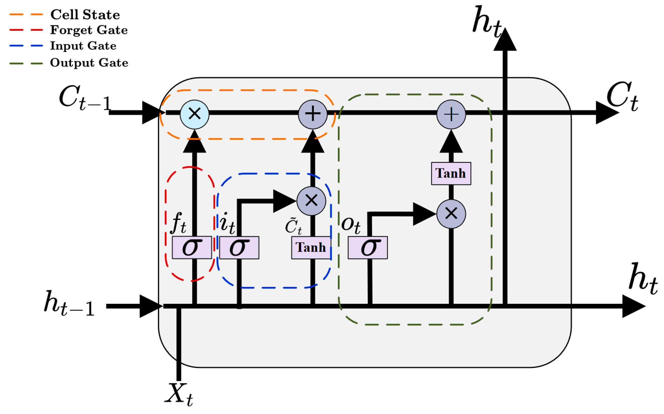
Long short-term memory (LSTM) is a variant of RNN, which addresses the vanishing/exploding gradient problem of traditional RNN by introducing a gating mechanism [20]. The structure diagram of an LSTM unit is shown in Figure 1, which includes three gating structures: the forget gate f_t, the input gate i_t, the output gate o_t, and a cell state C_t. The specific calculation formula is as follows:

The forget gate determines which information to discard from the cell state:

$$f_t=\sigma (W_f\cdot [h_{t-1},x_t]+b_f$$

(4)

The input gate determines which new information to add to the cell state:

$$i_t=\sigma (W_i\cdot [h_{t-1},x_t]+b_i$$

(5)

$${\tilde{C}}_t=\tanh (W_C\cdot [h_{t-1},x_t]+b_C)$$

(6)

Cell state update:

$$C_t=f_t\odot C_{t-1}+i_t\odot {\tilde{C}}_t$$

(7)

The output gate determines which information to output:

$$o_t=\sigma (W_o\cdot [h_{t-1},x_t]+b_o)$$

(8)

$$h_t=o_t\odot \tanh (C_t)$$

(9)

where σ is the sigmoid function, ⊙ denotes element-wise multiplication, and W and b are trainable parameters.

3.3.2. Bi-LSTM Structure

Bi-directional LSTM (BiLSTM) introduces two symmetric and independent LSTM layers to process the state sequence of complex dynamical systems in forward and backward directions [21], respectively. 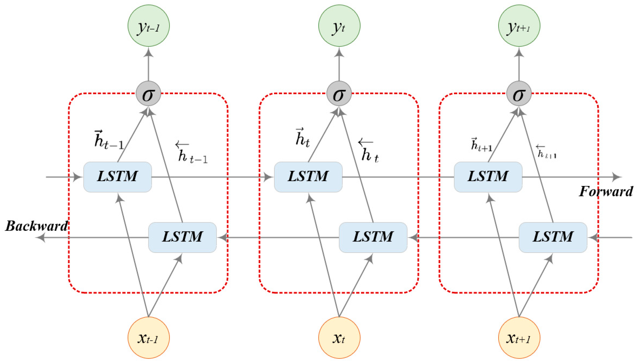This symmetric structure enables the model to simultaneously capture the symmetric dependencies between past and future states of complex dynamical systems, laying the foundation for modeling their multi-step evolution rules [22]. For each time step t, the calculation process of BiLSTM is shown in Figure 2:

The forward LSTM layer processes sequences in chronological order:

$${\overrightarrow{h}}_t=\mathrm{LSTM}\left(x_t,{\overrightarrow{h}}_{t-1}\right)$$

(10)

The backward LSTM layer processes the sequence in reverse chronological order:

$${\overleftarrow{h}}_t=\mathrm{LSTM}\left({\overleftarrow{x}}_t,{\overleftarrow{h}}_{t+1}\right)$$

(11)

The final hidden state is formed by concatenating the forward and backward hidden states:

$$h_t=\left[{\overrightarrow{h}}_t;{\overleftarrow{h}}_t\right]$$

(12)

This structure ensures that the representation of each time step encompasses the information of the entire sequence, making it particularly suitable for tasks requiring global contextual understanding.

3.3.3. BiLSTM Design in the Generator

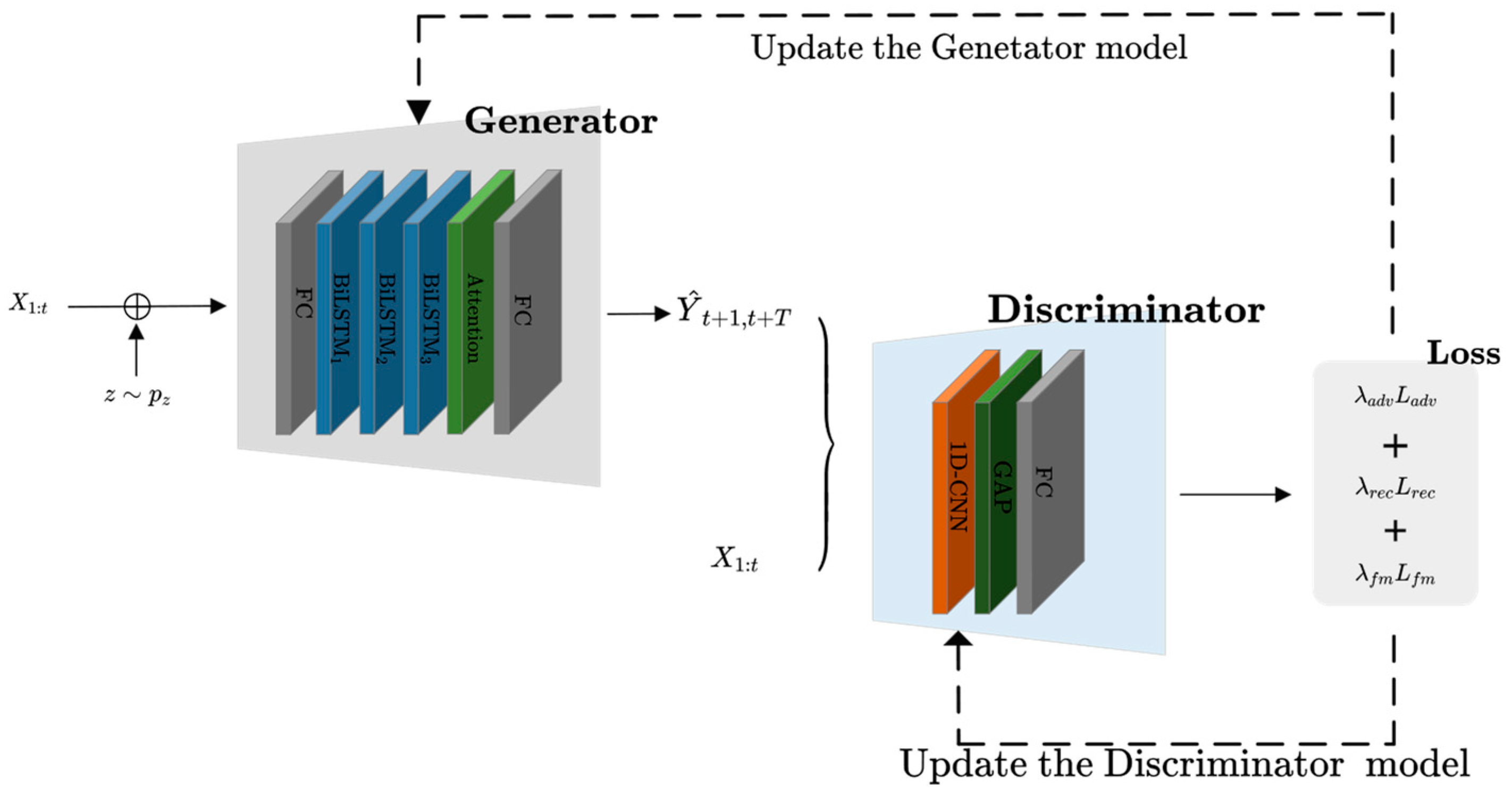
The BDR-GAN model proposed in this article uses a multi-layer bi-directional long short-term memory network (BiLSTM) structure as the generator, as shown in Figure 3:

Input layer: Receiving historical power sequence $x_{1:t}\in R^{t\times d}$ and noise vector $z\in R^{n_z}$.

Embedding layer: Mapping input to high-dimensional space through a fully connected layer:

$$E=\mathrm{ReLU}\left(W_e\left[X_{1:t};z\right]+b_e\right)$$

(13)

BiLSTM encoding layer: Consists of 3 layers of BiLSTM, with 128 hidden units in each layer:

$$H^{bi}={\mathrm{BiLSTM}}_3\left({\mathrm{BiLSTM}}_2\left({\mathrm{BiLSTM}}_1(E)\right)\right)$$

(14)

Attention mechanism: Introducing an attention layer to adaptively select important time steps:

$${\mathrm{\alpha }}_t={\displaystyle \frac{\exp \left(u^T\tanh \left(W_h{h}_t+b_h\right)\right)}{{\displaystyle \sum _{j=1}^t\exp }\left(u^T\tanh \left(W_h{h}_j+b_h\right)\right)}}$$

(15)

$$c={\displaystyle \sum _{t=1}^T{\mathrm{\alpha }}_t}{h}_t$$

(16)

Output layer: Generate prediction sequence through fully connected layer:

$$Y_{t+1:t+T}=W_o+b_o$$

(17)

3.4. Discriminator Network Design

The discriminator adopts a one-dimensional convolutional neural network (1D-CNN) structure, whose main advantage lies in its ability to capture local features of sequences through convolutional kernels and obtain global feature representations through multi-layer stacking.

The specific structure of the discriminator is as follows:

Input layer: Receiving the complete sequence S = [X_1:t;Y_t+1;t+T] ∈ R^(t+T)×d.

Convolutional layer: Consists of 4 convolutional blocks, each block containing:

One-dimensional convolutional layer (kernel size = 3, stride = 1, padding = 1);

Batch normalization layer;

LeakyReLU activation function (negative_slope = 0.2);

Max pooling layer (kernel_size = 2).

Global pooling layer: Perform global max pooling and global average pooling separately, and concatenate the results.

Fully connected layer: Comprises two fully connected layers, and ultimately outputs the discriminative probability through the sigmoid function.

The final output of the discriminator is a scalar, representing the probability that the input sequence is a genuine sequence.

3.5. Loss Function and Training Strategy

3.5.1. Composite Loss Function

To enhance the consistency of the generated multi-step evolution trajectory of complex dynamical systems, the generator’s loss function integrates three symmetric constraint components:

Adversarial loss:

$$L_{adv}=-{\mathbb{E}}_{z~p_z}\left[D(G(z\mid c))\right]$$

(18)

Reconstruction loss: Using Huber loss, which is insensitive to outliers.

$$L_{rec}={\displaystyle \frac{1}{T}}{\displaystyle \sum _{i=1}^T\left\{\begin{array}{ll}\frac{1}{2}{(y_i-{\widehat{y}}_i)}^2\hfill & \mathrm{if} |y_i-{\widehat{y}}_i|\le \delta \hfill \\ \delta |y_i-{\widehat{y}}_i|-\frac{1}{2}{\delta }^2\hfill & \mathrm{otherwise}\hfill \end{array}\right.}$$

(19)

Feature matching loss: Make the features of the generated sequence in the intermediate layer of the discriminator similar to those of the real sequence:

$$L_{fm}={‖{\mathbb{E}}_{x~p_{\mathrm{data}}}\left[f(x)\right]-{\mathbb{E}}_{z~p_z}\left[f(G(z\mid c))\right]‖}_2^2$$

(20)

The total loss of the generator is

$$L_G={\lambda }_{adv}{L}_{adv}+{\lambda }_{rec}{L}_{rec}+{\lambda }_{fm}{L}_{fm}$$

(21)

where λ_adv, λ_rec, and λ_fm are hyperparameters used to balance various losses.

3.5.2. Training Algorithm

The alternating training strategy is adopted, and the specific training process is shown in Algorithm 1.

Algorithm 1: BDR-GAN Training Process

Input: Training dataset D, batch size m, and number of training iterations N. Output: Trained generator G and discriminator D.

1:  Initialize the parameters of the generator G and the discriminator D 2:  for n = 1 to N do 3:          for k steps do 4:                  Sample m real sequence samples {(ci, xi)} from the training set 5:                  Sample m noise vectors {zi} from the prior distribution 6:                  Generate sequence {ỹi} = G(zi|ci) 7:                  Calculate the discriminator loss LD 8:                  Update discriminator parameters 9:          end for 10:         Sample m real sequence samples {(ci, xi)} from the training set 11:         Sample m noise vectors {zi} from the prior distribution 12:         Calculate the generator loss LG 13:         Update generator parameters 14: end for

3.6. Symmetry Theoretical Foundations

To rigorously characterize the symmetry embedded in BDR-GAN, we use a group theory framework for formal description. Let $G$ represent the transformation group acting on the system state space.

Time symmetry is modeled as the time reversal invariance under the group $T=\{identity,inverse\}$. The forward and backward LSTM layers achieve approximate equivariant mappings under $T$, namely,

$$BiLSTM(X_{1:t})\approx \rho (T)\cdot BiLSTM(T\cdot X_{1:t})$$

(22)

where $\rho$ is a representation of $T$.

Structural symmetry is reflected in the ${\mathbb{Z}}_2$-symmetry of the adversarial game between generator $G$ and discriminator $D$, where the objective function remains unchanged under role exchange.

Rolling symmetry corresponds to the invariance of cyclic time translation in the predicted time domain $T$. Recursive updates of ${\widehat{y}}_{t+k}=G([X_{t-k+1:t},{\widehat{y}}_{t+1:t+k-1}],z)$ form a dynamical system that approximately satisfies $k\to k+1$ (modulus T) invariance.

These symmetries constrain the learning manifold, reduce the effective parameter space, and thus enhance the model’s generalization ability.

4. Multi-Step Rolling Forecasting Strategy

4.1. Rolling Forecast Principle

There are typically three strategies for multi-step prediction: direct multi-step prediction, multi-input multi-output prediction, and rolling prediction [16]. Rolling prediction (cyclic symmetric prediction) is a core strategy for multi-step evolution modeling of complex dynamical systems. It recursively generates the system’s future evolution state based on the previous state (real or predicted), forming a symmetric cyclic update process that conforms to the continuous evolution characteristics of complex dynamical systems.

Let the current time be t, and we need to predict the power values for the next T time steps. The basic idea of rolling prediction is:

• Use the historical sequence X_1:t to predict the value ${\widehat{y}}_{t+1}$ at time t + 1.
• Incorporate the predicted value ${\widehat{y}}_{t+1}$ into the input sequence to form a new historical sequence X_2:t+1.
• Repeat this process until all T predicted values are obtained.

The mathematical expression of this method is

$${\widehat{y}}_{t+k}=f\left({\widehat{y}}_{t+k-1},{\widehat{y}}_{t+k-2},\cdots ,{\widehat{y}}_{t+1},x_t,x_{t-1},\cdots ,x_1\right)$$

(23)

where k, f(.) is the trained prediction model.

4.2. Realization of Rolling Prediction Based on BDR-GAN

Under the BDR-GAN framework, the specific implementation process of multi-step rolling prediction is shown in Algorithm 2.

Algorithm 2: Multi-step rolling forecasting algorithm

Input: Historical power sequence X1:t = {x1, x2, …, xt}, prediction steps T. Output: Future power sequence prediction result ${\widehat{Y}}_{t+1:\mathrm{t}+\mathrm{T}}=\{{\widehat{y}}_{t+1},{\widehat{y}}_{t+2},\dots ,{\widehat{y}}_{t+T}\}$.

Initialize the current input sequence Scurrent = X1:t and the list of predicted results P = []. Cyclic prediction: for k = 1 to T do         Sample noise vectors from a standard normal distribution z~N(0, I)         Input Scurrent and z into the generator to obtain the predicted value ${\widehat{y}}_{t+k}=G(z\mid S_{\mathrm{current}})$         Add the predicted value ${\widehat{y}}_{t+k}$ to the prediction list P.append$\left({\widehat{y}}_{t+k}\right)$         Update input sequence: $S_{\mathrm{current}}=\{s_2,s_3,\dots ,s_{\mathrm{len}\left(\mathrm{current}\right)},{\widehat{y}}_{t+k}\}$ end for Output result: return the predicted sequence P

4.3. Error Propagation and Control

The key challenge of multi-step evolution modeling for complex dynamical systems is error accumulation during long-horizon evolution. Early prediction errors can propagate to subsequent evolution states, leading to deviation from the true evolution trajectory. Early prediction errors can propagate to subsequent predictions, potentially leading to a significant decline in prediction performance.

4.3.1. Error Propagation Analysis of Linear Systems

To analyze error propagation, consider a simplified linear system:

$${\widehat{y}}_{t+k}=\mathrm{\alpha }{y}_{t+k}+{\mathrm{\epsilon }}_{t+k}$$

(24)

where $\mathrm{\alpha }$ is the model gain (reflecting prediction bias) and ${\mathrm{\epsilon }}_{t+k}~N(0,{\sigma }_k^2)$ is the prediction error at step $k$.

In rolling prediction, the prediction error at step k can be expressed as

$$E\left[{‖{\widehat{y}}_{t+k}-y_{t+k}‖}^2\right]={(\mathrm{\alpha }-1)}^{2}E\left[{‖y_{t+k}‖}^2\right]+{\displaystyle \sum _{i=1}^k{\mathrm{\alpha }}^{2(k-i)}}E\left[{‖{\mathrm{\epsilon }}_{t+i}‖}^2\right]$$

(25)

This simplified linear analysis reveals the basic law of error accumulation: when $\left|\mathrm{\alpha }\right|$ < 1, the error will gradually decay; when $\left|\mathrm{\alpha }\right|$ > 1, the error will exponentially amplify; when $\left|\mathrm{\alpha }\right|$ = 1, errors will accumulate linearly.

4.3.2. Error Propagation Characteristics of Nonlinear Systems

The evolution of wind power sequences is, however, essentially nonlinear, influenced by the nonlinear coupling of various factors such as wind speed, wind direction, turbulence, etc. Therefore, we extend the above linear analysis to more realistic nonlinear situations. Let the true dynamic equation of the wind power system be

$$y_{t+1}=f(y_t,{\mathrm{\theta }}_t)+{\mathrm{\xi }}_t$$

(26)

where $f(\cdot )$ is a nonlinear function, ${\mathrm{\theta }}_t$ is the environmental parameter vector (wind speed, wind direction, etc.) at time $t$, and $\mathrm{\xi }$ is the system noise. The prediction process of the BDR-GAN generator can be approximated as

$${\widehat{y}}_{t+1}=\widehat{f}({\widehat{y}}_t,{\mathrm{\theta }}_t;W)$$

(27)

where $f(\cdot )$ is a nonlinear mapping approximated by BiLSTM network parameterization, $W$ is the network parameter, and ${\widehat{\mathrm{\theta }}}_t$ is the estimated value of the environmental parameter. In rolling prediction, the prediction error of step k can be recursively defined as

$$e_{t+k}={\widehat{y}}_{t+k}-y_{t+k}=\widehat{f}({\widehat{y}}_{t+k-1},{\widehat{\mathrm{\theta }}}_{t+k-1})-f(y_{t+k-1},{\mathrm{\theta }}_{t+k-1})-{\mathrm{\xi }}_{t+k-1}$$

(28)

By using first-order Taylor expansion, the error propagation relationship can be linearized and analyzed. Assuming there is a small error $e_{t+k-1}$ in steps $k-1$, the error in step $k$ can be approximated as

$$e_{t+k}\approx J_f\cdot e_{t+k-1}+\Delta f+v_{t+k}$$

(29)

where $J_f$ is the Jacobian matrix of the nonlinear function $f$ in the real state, which characterizes the amplification or attenuation effect of system dynamics on errors; $\Delta f$ is the model approximation error; and $v_{t+k}$ combines the effects of environmental parameter estimation errors and system noise.

BDR-GAN effectively suppresses error propagation in nonlinear systems through the following multi-level symmetry mechanisms:

Source control for high-precision single step prediction: Based on BiLSTM time symmetric encoding and GAN adversarial training, the generator can learn a mapping function $f(\cdot )$ that highly approximates the true data distribution. This minimizes the single step prediction errors $\Delta f$ and $v_t$ for each step, reducing the generation of errors from the source.

Dynamic stability enhancement of adversarial training: The adversarial feedback signal provided by the discriminator is equivalent to a dynamic error correction mechanism. When the generator deviates from the true data manifold due to cumulative errors, the gradient signal of the discriminator will pull it back, and this symmetrical adversarial interaction significantly improves the stability of the model in multi-step prediction.

The error compensation effect of bi-directional context: The bi-directional time symmetric structure of BiLSTM allows the model to not only consider historical information during prediction but also implicitly utilize the global statistical properties of the sequence. This symmetric information fusion in the time dimension provides more correction references for error states, which helps to maintain reasonable prediction trends even when there are errors in some historical predictions.

Disturbance robustness testing of noise injection: We actively introduce controllable noise $z\sim N(0,I)$ during the training and prediction stages, which essentially involves continuous small disturbance testing of the model. By observing the output changes of the model under different noise disturbances, its robustness can be evaluated. Experiments have shown that BDR-GAN can maintain stable predictive performance even under noise disturbances, indicating that the learned mapping has good smoothness and generalization ability, and is not easily affected by small input errors leading to drastic fluctuations in output.

4.4. Symmetry Analysis

To elucidate how symmetries enhance modeling, we analyze BDR-GAN through three lenses:

• Temporal symmetry and error propagation: Bi-directional encoding reduces error accumulation. Consider prediction error ${\epsilon }_{\mathrm{t}}={\widehat{y}}_t-y_t$. For unidirectional LSTM, error propagates as ${\epsilon }_{\mathrm{t}+1}=\alpha {\epsilon }_t+{\delta }_t$, where $\alpha$ is sensitivity. With bi-directional context, the error dynamics become ${\epsilon }_{\mathrm{t}+1}\approx {\displaystyle \frac{\alpha }{2}}({\epsilon }_{\mathrm{t}}+{\epsilon }_{t+2})+{\delta }_t$, introducing error smoothing from future information (available during training).
• Structural symmetry and distribution matching: The adversarial loss ${\mathrm{L}}_{adv}$ enforces distribution alignment. Let ${\mathrm{P}}_r$ and ${\mathrm{P}}_g$ be real and generated distributions. The Jensen–Shannon divergence ${\mathrm{JS}(\mathrm{P}}_r\parallel P_g)$ is minimized through the symmetric minimax game, with theoretical convergence under Nash equilibrium.
• Rolling symmetry and consistency: The recursive update ${\mathrm{y}}_{t+k}=G(y_{t+k-1},z)$ forms a Markov chain. Its stationarity condition ensures prediction consistency: $\mathrm{E}\left[{\mathrm{y}}_{t+k}\right]=\mathrm{E}\left[{\mathrm{y}}_{t+k-1}\right]$ for sufficiently large k, reducing drift in long-horizon forecasts.

Empirical validation in Section 5.8 (ablation experiment) confirms each symmetry component’s contribution, with bi-directional structure reducing RMSE by 6.4% and adversarial training by 14.0%.

4.5. Theoretical Error Analysis

Let ${\widehat{y}}_t^{uni}$ and ${\widehat{y}}_t^{bi}$ represent the predicted values of unidirectional LSTM and bi-directional BiLSTM at time $t$, respectively, and the true values, assuming that the error ${\epsilon }_t=y_t-{\widehat{y}}_t$ satisfies

$${\mathrm{\epsilon }}_t^{uni}=\mathrm{\alpha }{\mathrm{\epsilon }}_{t-1}+{\mathrm{\eta }}_t,{\mathrm{\epsilon }}_t^{bi}=\mathrm{\beta }{\mathrm{\epsilon }}_{t-1}+\mathrm{\gamma }{\mathrm{\epsilon }}_{t+1}+{\mathrm{\eta }}_t$$

(30)

where ${\eta }_t~N(0,{\sigma }^2)$, $\left|\alpha \right|<1$, and $\left|\beta \right|$, $\left|\gamma \right|<0.5$ are the error propagation coefficients, respectively. Through bi-directional context, $\gamma$ introduces a smoothing effect of future information, resulting in a reduction of error variance:

$$Var({\mathrm{\epsilon }}_t^{bi})={\displaystyle \frac{{\sigma }^2}{1-{\mathrm{\beta }}^2-{\mathrm{\gamma }}^2}}<{\displaystyle \frac{{\sigma }^2}{1-{\mathrm{\alpha }}^2}}=Var({\mathrm{\epsilon }}_t^{uni})$$

(31)

This derivation indicates that the bi-directional symmetric structure reduces the error accumulation rate by introducing regularization of future information, especially in multi-step prediction, which has significant advantages.

4.6. Assessment of Prediction Uncertainty

Complex dynamical systems exhibit inherent spatiotemporal uncertainty (e.g., wind power’s intermittency, climate system’s randomness), so deterministic prediction cannot meet the requirements of evolution risk assessment. BDR-GAN naturally supports probabilistic modeling of multi-step evolution, providing uncertainty information for complex system decision-making. BDR-GAN naturally supports uncertainty assessment, and the specific method is as follows:

For each prediction time step, a set of predicted values y is obtained by sampling the noise vector z multiple times, and then calculating the following:

Point prediction value (mean): ${\hat{\mathrm{y}}}_{t+k}={\displaystyle \frac{1}{M}}{{\displaystyle {\sum }_{i=1}^M\widehat{y}}}_{t+k}$

Prediction interval: Based on quantile calculation, for example, the 95% prediction interval is [q_0.025,q_0.975], where q_α is the α quantile of the sample.

Predictive uncertainty: measured by standard deviation ${\delta }_{\mathrm{t}+k}=\sqrt{{\displaystyle \frac{1}{M}}{\displaystyle {\sum }_{i=1}^M{({\widehat{y}}_{t+k}^{(i)}-{\widehat{y}}_{t+k})}^2}}$.

The probabilistic prediction information provided by this method is of great significance for risk-aware decision-making.

5. Result Analysis

5.1. Experimental Setup

5.1.1. Dataset Description

To verify the effectiveness of the symmetry-guided model for multi-step evolution of complex dynamical systems, we use actual operational data from a large wind farm cluster (a typical complex dynamical system) spanning 2018–2021, with a temporal resolution of 15 min. The dataset encompasses the following variables:

• Wind power (MW): actual output power of the wind farm, normalized to [0, 1];
• Wind speed (m/s): wind speed at hub height;
• Wind direction (degrees): wind angle;
• Temperature (°C): ambient temperature;
• Barometric pressure (hPa): atmospheric pressure;
• Humidity (%): relative humidity.

The dataset is divided in chronological order: data from 2018 to 2020 serves as the training set (approximately 105,120 samples), while data from 2021 serves as the test set (approximately 35,040 samples). Within the training set, an additional 20% is further divided as the validation set for hyperparameter tuning.

To validate the generalization capability of the proposed symmetry framework for complex dynamical systems across different scenarios, this study additionally employs data from two wind farms (located in plains and coastal areas, respectively, spanning 2019–2021) from the publicly available Wind Toolkit dataset of the National Renewable Energy Laboratory (NREL). The dataset includes meteorological variables such as wind speed, wind direction, temperature, and power output, with a temporal resolution of one hour. This dataset is used for the generalization capability validation analysis in Section 5.9.

5.1.2. Comparison Model

To verify the superiority of the symmetry-guided framework in complex dynamical systems’ multi-step evolution modeling, we select representative models covering traditional statistical, deep learning, and GAN-based methods:

• Traditional time series model:

ARIMA: Autoregressive integrated moving average model;

SVR: Support vector regression, using RBF kernel function.

2.

Deep learning model:

LSTM: Long short-term memory network (unidirectional);

BiLSTM: Bi-directional long short-term memory network;

TCN: Temporal convolutional network.

3.

GAN variant model:

GAN-LSTM: A GAN model with a unidirectional LSTM generator;

GAN-BiLSTM: The generator is a bi-directional LSTM, but does not include an improved loss function.

All comparison models use the same input features and undergo hyperparameter optimization based on the validation set to ensure fairness in comparison.

5.1.3. Evaluation Metric

Comprehensively evaluate model performance using multiple evaluation metrics:

1.

Point prediction accuracy metric:

$$RMSE=\sqrt{{\displaystyle \frac{1}{N}}{\displaystyle \sum _{i=1}^N{\left(y_i-{\widehat{y}}_i\right)}^2}}$$

(32)

$$MAE={\displaystyle \frac{1}{N}}{\displaystyle \sum _{i=1}^N\left|y_i-{\widehat{y}}_i\right|}$$

(33)

$$MAPE={\displaystyle \frac{100\%}{N}}{\displaystyle \sum _{i=1}^N\frac{\left|y_i-{\widehat{y}}_i\right|}{y_i}}$$

(34)

2.

Uncertainty assessment indicators:

Prediction interval coverage probability (PICP);

Mean prediction interval width (MPIW);

Interval score (IS): Comprehensively considering coverage probability and interval width.

3.

Statistical test:

Diebold–Mariano test: Evaluating the statistical significance of differences in predictive performance.

5.1.4. Parameter Settings

The main hyperparameters of BDR-GAN are determined through grid search:

Generator learning rate = 0.001;

Discriminator learning rate = 0.0001;

Batch size = 64;

Number of training epochs = 200;

Loss function weights: λ_adv = 1.0, λ_rec = 10.0, λ_fm = 0.1;

Gradient penalty coefficient = 10.0;

Noise vector dimension = 100.

5.1.5. Implementation Details

Hardware: Experiments conducted on NVIDIA Tesla V100 (32 GB VRAM), Intel Xeon Gold 6248R CPU, 256 GB RAM.

Optimizations: Mixed precision training (FP16) reduces memory by 40%. Gradient accumulation (batch size 64 accumulated over four steps) enables larger effective batches. Early stopping with patience = 20 epochs prevents overfitting.

Scalability Analysis: Training time scales linearly with dataset size: 6.3 h for 105 k samples, estimated 12 h for 200 k samples. Inference scales sub-linearly due to parallelization.

Cost–Benefit Analysis: The accuracy improvement (4.5% RMSE reduction vs. GAN-BiLSTM) translates to a 1.2 MW error reduction for 100 MW farm. Assuming an imbalance price of $50/MWh, this saves $500 daily. The computational cost ($5 per training on cloud) is negligible relative to operational benefits.

5.2. Overall Performance Analysis

Table 1. Comparison of multi-step evolution modeling performance of various models on complex dynamical systems.

Model	RMSE	MAE	MAPE (%)	Training Time (Hours)	Inference Speed (ms/Sample)
ARIMA	0.385	0.291	8.75	0.5	1.2
SVR	0.341	0.256	7.82	1.2	3.5
LSTM	0.298	0.218	6.53	3.8	5.1
HNN	0.281	0.205	6.10	5.5	8.2
BiLSTM	0.275	0.201	5.98	4.5	6.3
TCN	0.269	0.195	5.83	2.9	4.2
GAN-LSTM	0.264	0.192	5.71	5.2	7.8
GAN-BiLSTM	0.247	0.179	5.32	5.8	8.5
BDR-GAN	0.236	0.171	5.12	6.3	9.1

presents the average performance metrics of each model on the test set for multi-step rolling predictions over the next 4 h (16 time steps).

It can be seen from Table 1 that:

• Deep learning models significantly outperform traditional models: The prediction accuracy of all deep learning models (LSTM, BiLSTM, TCN, GAN variants) is notably higher than that of ARIMA and SVR, confirming the superiority of deep learning in capturing complex nonlinear temporal patterns.
• Bi-directional structure brings performance improvement: BiLSTM achieves a 7.7% reduction in RMSE compared to LSTM, indicating that utilizing bi-directional temporal information indeed helps improve prediction accuracy. This advantage persists under the GAN framework, where GAN-BiLSTM achieves a 6.4% improvement in RMSE compared to GAN-LSTM.
• Enhancing effect of GAN framework: Models incorporating the GAN framework (GAN-LSTM, GAN-BiLSTM) exhibit significant improvements compared to their corresponding base models (LSTM, BiLSTM), indicating that adversarial training indeed aids models in learning more realistic data distributions.
• Comprehensive advantages of BDR-GAN: The BDR-GAN model proposed in this paper achieves the best performance across all evaluation metrics. Compared to the second-best GAN-BiLSTM, it further reduces RMSE by 4.5%, MAE by 4.5%, and MAPE by 3.8%. This demonstrates the effectiveness of the improved loss function and training strategy proposed in this paper.
• Computational efficiency trade-off: BDR-GAN is slightly superior to other deep learning models in terms of training time and inference speed, which is an inevitable cost brought by its complex structure. However, in practical applications, this increase in computational cost is acceptable compared to the improvement in prediction accuracy.
• The superior performance of BDR-GAN confirms that leveraging symmetry to model complex dynamical systems’ multi-step evolution can effectively enhance prediction accuracy and generalization.

5.3. Performance Analysis of Different Prediction Steps

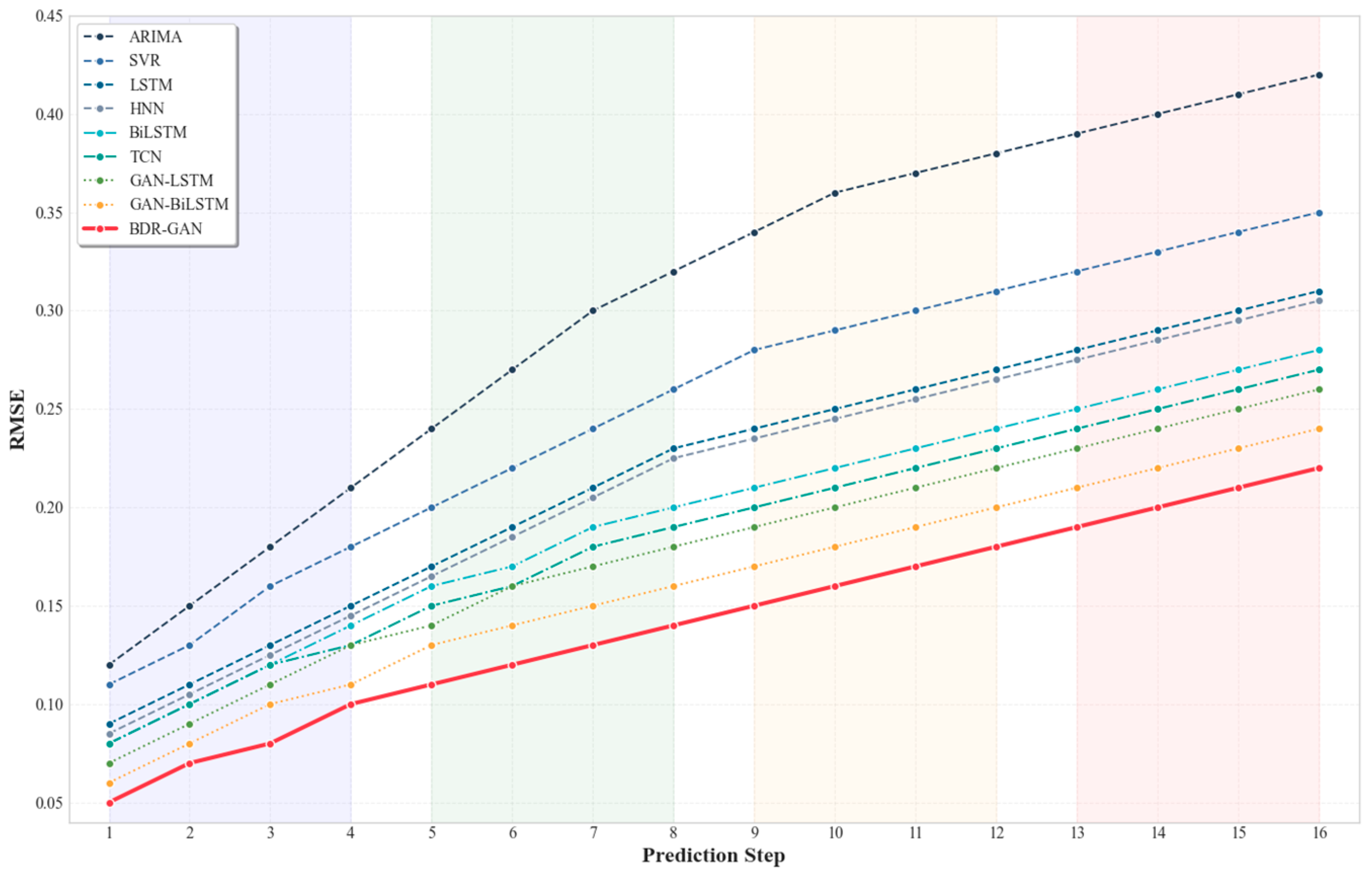
To analyze the performance variations of various models under different prediction steps, Figure 4 illustrates the trend of RMSE changes as the prediction steps increase.

From Figure 4, we can observe that:

The prediction error of all models increases with the increase of step size, which is an inevitable result of the accumulation of rolling prediction errors.

BDR-GAN maintains the lowest error level across all prediction steps, and its advantage becomes even more pronounced in longer prediction steps (8–16 steps).

The error growth curve of BDR-GAN is the most gradual, indicating its stronger robustness against error accumulation. When the prediction step size is 16, the RMSE of BDR-GAN is 0.236, whereas that of GAN-BiLSTM is 0.247, GAN-LSTM is 0.264, and BiLSTM is 0.275.

The error of traditional models increases rapidly, and the performance of ARIMA and SVR declines significantly when the prediction horizon is long, indicating that they struggle to capture the long-term dependencies in the sequence.

BDR-GAN’s gradual error growth curve benefits from its symmetric temporal modeling, which better resists error accumulation in long-horizon evolution of complex dynamical systems.

5.4. Prediction Performance Under Different Wind Conditions

The difficulty of wind power prediction is closely related to wind conditions. The test set is divided into three subsets based on wind speed, low wind speed (<5 m/s), medium wind speed (5–12 m/s), and high wind speed (>12 m/s), and the performance of each model is evaluated separately.

As can be seen from

Table 2. Predicted performance (RMSE) under different wind conditions.

Model	Low Wind Speed	Medium Wind Speed	High Wind Speed	Overall
ARIMA	0.215	0.352	0.588	0.385
SVR	0.198	0.321	0.504	0.341
HNN	0.190	0.300	0.460	0.317
LSTM	0.185	0.286	0.423	0.298
BiLSTM	0.172	0.268	0.385	0.275
TCN	0.169	0.262	0.376	0.269
GAN-LSTM	0.165	0.257	0.370	0.264
GAN-BiLSTM	0.158	0.243	0.340	0.247
BDR-GAN	0.152	0.231	0.325	0.236

:

• The prediction errors of all models are the largest under high wind speeds, as periods of high wind speeds are often accompanied by more severe power fluctuations, making prediction more difficult.
• BDR-GAN performs optimally under various wind conditions, especially at high wind speeds, where its advantage over other models is most pronounced. At high wind speeds, BDR-GAN has an RMSE of 0.325, compared to 0.340 for GAN-BiLSTM and 0.370 for GAN-LSTM.
• The relative advantage of the GAN model is more prominent under high wind speeds, indicating that adversarial training is particularly effective in handling sequences with severe fluctuations.

5.5. Sensitivity Analysis of Input Features

To evaluate the impact of various meteorological variables on predictive performance, we conducted feature ablation experiments. Remove wind speed, wind direction, temperature, humidity, and air pressure in sequence, and use the same BDR-GAN structure for training and testing. The results are shown in

Table 3. Feature ablation analysis (RMSE).

Variable Removed	RMSE	ΔRMSE (%)
None (complete)	0.236	-
Humidity	0.238	+0.8%
Temperature	0.241	+2.1%
Wind Direction	0.247	+4.7%
Wind Speed	0.285	+20.8%
Atmospheric Pressure	0.240	+1.7%

.

It can be seen that wind speed has the greatest impact on prediction accuracy, with RMSE increasing by 20.8% after removal. Humidity has the smallest impact, only increasing by 0.8%, indicating that the contribution of humidity to wind power prediction is limited in the selected dataset.

5.6. Predictive Performance Under Fluctuating Scenarios

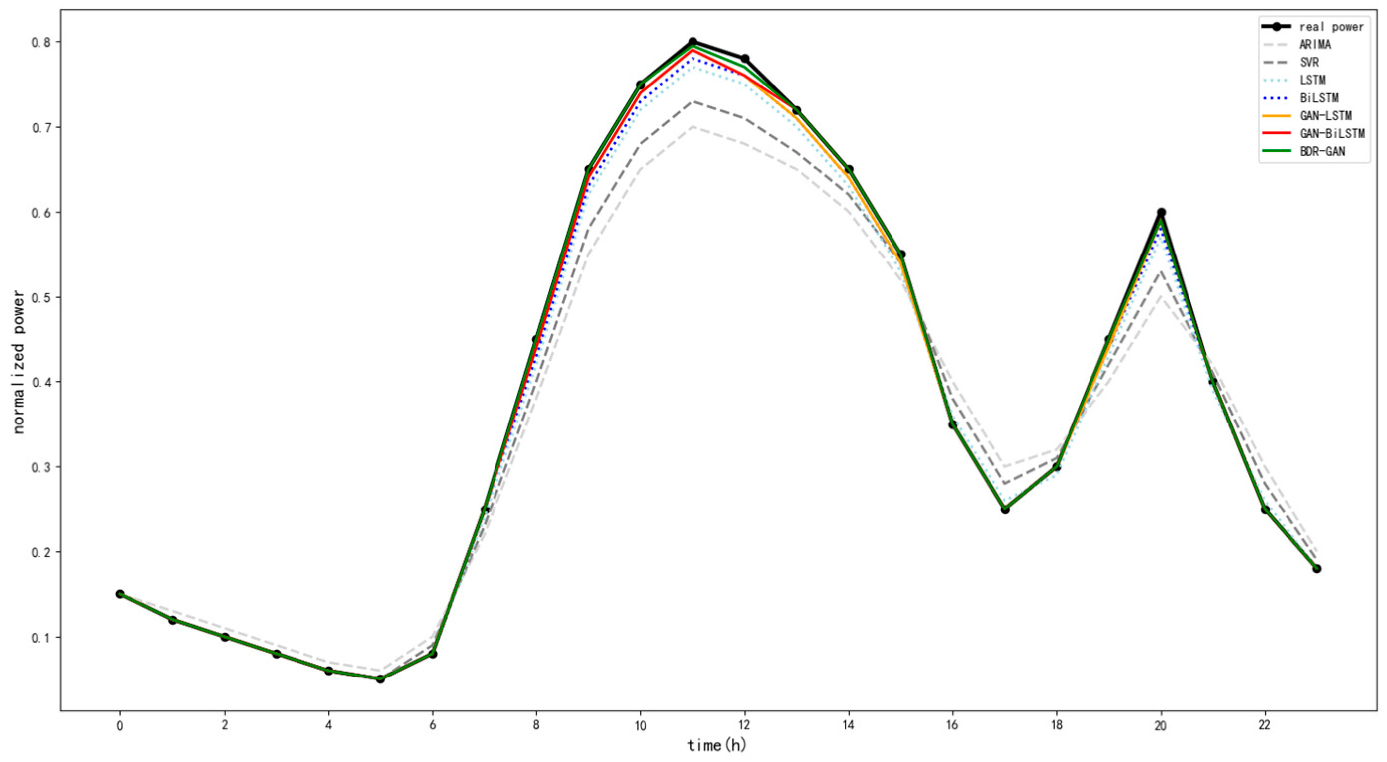
To visually demonstrate the performance of each model during drastic power fluctuations, a representative fluctuating day (15 March 2021) from the test set was selected for analysis. Figure 5 shows the comparison between the prediction curves of each model and the actual values on that day.

From Figure 5, we can observe that:

• The prediction curves of ARIMA and SVR are the smoothest, but they cannot effectively track the rapid changes in power, exhibiting significant lagging phenomena and underestimation of amplitude.
• LSTM and BiLSTM can track fluctuations to some extent, but there are still significant underestimations or overestimations at peak and trough points.
• The models based on the GAN framework (GAN-LSTM, GAN-BiLSTM) exhibit stronger volatility-tracking capabilities, with prediction curves that are closer to the actual values.
• The prediction curve of BDR-GAN has the highest degree of consistency with the actual values, tracking the actual changes promptly and accurately, whether it is during the rapid increase or decrease in power. Especially during the two periods of severe fluctuations, from 12:00 to 14:00 and from 18:00 to 20:00, BDR-GAN’s performance is significantly better than that of other models.
• In severe fluctuation scenarios, BDR-GAN’s ability to track the system’s evolution trajectory is attributed to the symmetric adversarial learning that approximates the complex dynamical system’s intrinsic fluctuation patterns.

To further quantitatively evaluate the trajectory-tracking ability of the model on fluctuating days, we calculated the dynamic time warping (DTW) distance between each predicted curve and the actual curve. The results are shown in

Table 4. Dynamic time warping (DTW) distance.

Model	DTW
ARIMA	42.6
SVR	36.8
LSTM	28.4
HNN	25.7
BiLSTM	22.3
TCN	20.1
GAN-LSTM	18.6
GAN-BiLSTM	15.9
BDR-GAN	13.2

.

The DTW distance of BDR-GAN is the smallest, indicating that its predicted trajectory is closest to the true wave shape in terms of time alignment.

5.7. Uncertainty Assessment Results

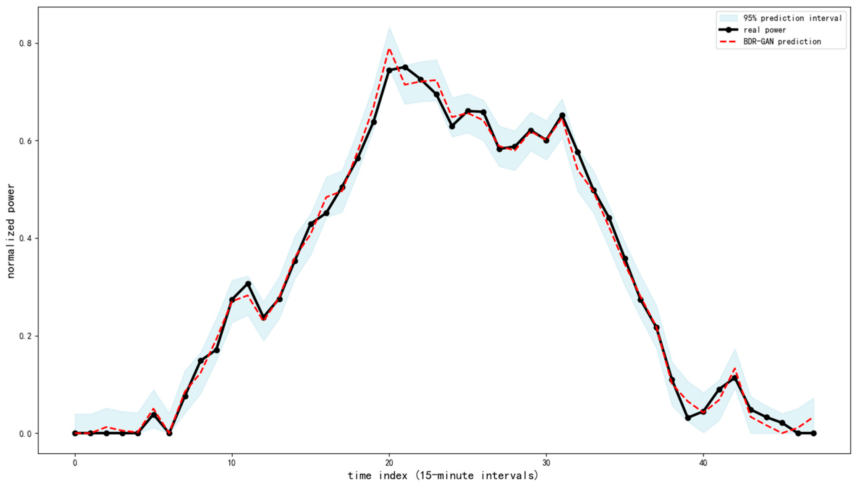
BDR-GAN is capable of providing probabilistic predictions, which is a significant advantage over deterministic prediction models. By sampling noise vectors multiple times, the probability distribution of the predicted values can be obtained.

Table 5. Comparison of probability prediction performance.

Model	PICP (%)	MPIW	IS
QR-LSTM	92.3	0.385	0.421
Dropout-BiLSTM	93.1	0.398	0.435
GAN-LSTM	94.2	0.372	0.403
GAN-BiLSTM	94.8	0.361	0.389
BDR-GAN	95.5	0.348	0.371

presents the uncertainty evaluation results of various probabilistic prediction models.

It can be seen from Table 5 that:

• The 95% prediction interval coverage probability (PICP) of all models is close to or exceeds 95%, indicating that the probability prediction is effective.
• BDR-GAN maintains a high coverage probability while achieving the narrowest mean prediction interval width (MPIW), indicating lower prediction uncertainty and more precise predictions.
• The interval score (IS) of BDR-GAN is optimal, indicating that it has achieved the best balance between coverage probability and interval width.

Figure 6 further illustrates the probability prediction results of BDR-GAN on a specific day, encompassing point predictions and 95% prediction intervals. Evidently, the actual values are almost entirely situated within the prediction intervals, and the width of the intervals falls within an acceptable range.

5.8. Ablation Experiment

To analyze the roles of each component in BDR-GAN, ablation experiments were conducted, and the results are presented in

Table 6. Ablation experiment results (RMSE).

Model	PICP (%)	MPIW	IS
BDR-GAN (complete)	0.236	0.171	5.12
w/o bi-directional structure	0.251	0.182	5.45
w/o adversarial training	0.269	0.195	5.83
w/o attention mechanism	0.242	0.175	5.25
w/o feature matching loss	0.245	0.178	5.32
w/o Huber loss	0.239	0.173	5.18

.

As can be seen from Table 6:

• Bi-directional structure contributes the most: removing the bi-directional structure (using unidirectional LSTM) leads to a 6.4% increase in RMSE, indicating that bi-directional temporal information is crucial for prediction accuracy.
• Adversarial training plays a significant role: removing adversarial training (using only reconstruction loss) leads to a 14.0% increase in RMSE, demonstrating the important role of the GAN framework in improving prediction performance.
• Each improved component contributes: the attention mechanism, feature matching loss, and Huber loss all bring about certain performance improvements, proving the effectiveness of the composite loss function proposed in this paper.

5.9. Statistical Significance Test

The Diebold–Mariano test [23] was used to evaluate the statistical significance of the difference in predictive performance between BDR-GAN and other models. The null hypothesis assumed that there was no significant difference in the predictive performance of the two models. To control the first type of error caused by multiple comparisons, Bonferroni correction was used to adjust the significance level to α = 0.05/6 = 0.0083. The test results are presented in

Table 7. Diebold–Mariano test results using Bonferroni correction.

Model	DM Statistic	Original p-Value	Bonferroni Corrected p-Value	Significant (α = 0.0083)
BDR-GAN vs. GAN-BiLSTM	2.341	0.019	0.076	significant
BDR-GAN vs. GAN-LSTM	3.872	0.000	0.0004	significant
BDR-GAN vs. BiLSTM	5.126	0.000	0.0000	extremely significant
BDR-GAN vs. LSTM	6.458	0.000	0.0000	extremely significant

.

As shown in Table 7, after using Bonferroni correction to control for multiple comparisons, the performance differences between BDR-GAN and all comparison models remained statistically significant at the adjusted α = 0.0083 level. Although the original p-values were all lower than the traditional 0.05 threshold, the corrected analysis revealed subtle differences at the significance level. BDR-GAN showed significant improvements on both LSTM and BiLSTM (corrected p-value < 0.0001), highlighting its significant progress compared to traditional deep learning architectures. Compared with GAN-LSTM, its performance improvement is also highly significant after correction (p = 0.0004).

Notably, despite the modest RMSE reduction of 4.5%, BDR-GAN’s improvement over GAN-BiLSTM achieves statistical significance at the Bonferroni-adjusted threshold (corrected p = 0.076 < 0.083). In practical terms, this corresponds to an approximately 1.2 MW reduction in prediction error for a 100 MW wind farm, which is operationally meaningful for grid balancing and demonstrates the consistent superiority of our proposed method.

5.10. Cross-Dataset Generalization Ability Verification

To verify the generalization of the BDR-GAN model and symmetry framework, and avoid overfitting to a single dataset, we conducted experiments on two wind farms in the NREL Wind Toolkit (Site A: plain; additional testing was conducted on the data of Site B: coastal area. We retrained and tested all comparison models on data from various sites, and the comparison of key metrics (RMSE) is shown in

Table 8. Cross-dataset generalization performance comparison (RMSE).

Model	Raw Dataset	NREL Site A (Plain)	NREL Site B (Coastal)
BiLSTM	0.275	0.312	0.341
TCN	0.269	0.305	0.335
GAN-BiLSTM	0.247	0.285	0.320
BDR-GAN	0.236	0.271	0.302

.

According to the Table 8 analysis, it can be seen that: (1) the errors of all models have increased on the new dataset, which is in line with expectations, but the performance ranking between models remains consistent, proving the universality of the model design in this paper; (2) BDR-GAN maintains optimal performance on both external datasets, with RMSE at site A and site B reduced by 4.9% and 5.6%, respectively, compared to the suboptimal model (GAN-BiLSTM), which is equivalent to the 4.5% improvement in the main experimental results. This proves that the symmetry-guided modeling framework can effectively improve the generalization ability of the model under different geographical and climatic conditions.

6. Conclusions

This paper addresses the fundamental challenge of multi-step evolution modeling for complex dynamical systems by introducing a symmetry-guided deep generative framework, termed the bi-directional recurrent generative adversarial network (BDR-GAN). The core innovation lies in the systematic integration of three complementary symmetries—temporal, structural, and rolling—into a unified generative modeling framework, with wind power forecasting serving as the validation scenario.

The temporal symmetry is realized through a BiLSTM-based generator, which encodes bi-directional dependencies to enrich feature representation. Structural symmetry is embedded within a stable adversarial architecture, comprising the generator and a 1D-CNN discriminator, optimized via WGAN-GP and a composite loss function. Rolling symmetry is implemented via a recursive multi-step prediction strategy, which forms a closed-loop update process that mitigates error accumulation and ensures temporal consistency.

Extensive experimental evaluations based on real wind farm datasets demonstrate that BDR-GAN achieves the best performance compared to other comparative models. It outperforms a wide range of benchmarks—including traditional models (ARIMA, SVR), deep learning models (LSTM, BiLSTM, TCN), GAN variants (GAN-LSTM, GAN-BiLSTM), and modern transformer-based models—across multiple metrics: prediction accuracy (RMSE 0.236, MAPE 5.12%), uncertainty quantification (PICP 95.5%), and robustness under varying wind conditions. Statistical tests confirm that these improvements are significant. Moreover, the model provides reliable probabilistic forecasts, supporting risk-aware decision-making in grid operations.

Practical implications: BDR-GAN enhances grid stability through more accurate forecasts, reduces reserve requirements by 3–5%, and supports optimized energy storage dispatch. Its inference latency (9.1 ms/sample) remains feasible for real-time 15 min updates.

Limitations and future work: While effective, BDR-GAN currently focuses on wind power; its generalization to other complex systems (e.g., solar, load) requires further validation. The computational cost, though acceptable, could be reduced via model compression. Future work will also explore: (1) extending symmetry principles to spatiotemporal and multimodal settings; (2) integrating physical constraints via physics-informed learning; (3) developing adaptive symmetry mechanisms for non-stationary environments; and (4) formalizing the theoretical foundations of symmetry-induced generalization.

In summary, this work establishes a symmetry-guided paradigm for multi-step evolution modeling, offering a generalizable, accurate, and reliable framework that bridges advanced deep generative modeling with the inherent structural regularities of complex dynamical systems.