Interval-Valued Picture Fuzzy Soft Rough Sets: A New Hybrid Framework for Robust Multi-Criteria Group Decision-Making

Abstract

This paper introduces a novel hybrid framework called Interval-Valued Picture Fuzzy Soft Rough Sets (IVPFSRS) designed to address complex uncertainty in multi-criteria group decision-making (MCGDM) problems. The model achieves a synergistic integration of three powerful mathematical theories: interval-valued picture fuzzy sets (IVPFS) for representing nuanced, interval-valued degrees of membership, neutrality, and non-membership; soft sets for parameterized problem formulation; and rough sets for handling data granularity and approximation under incompleteness. We formally define the IVPFSRS framework, investigate its fundamental properties and algebraic operations, and develop a comprehensive MCGDM algorithm with explicit weight incorporation to address the critical role of criterion importance. The effectiveness and robustness of the proposed approach are demonstrated through a detailed illustrative example of administrative position selection and a systematic comparative analysis with existing models. Results show that the IVPFSRS framework provides a more powerful, flexible, and logically coherent tool for robust decision making in highly uncertain and information-deficient environments. The proposed framework complements recent advancements in cloud-rough integration for large group decision making while offering unique advantages in parameterized three-way uncertainty representation and structured multi-criteria evaluation.

1. Introduction

In daily life, we encounter many complicated problems involving different types of uncertainties and ambiguities, as well as incomplete information. The classical mathematical tools, based on exact numerical data and deterministic procedures, are generally not suitable to address such issues, due to the problems involved being fuzzy and human in nature. The need for the extension of classical mathematical methodologies to deal with uncertainty in real applications has led to the design of various mathematical theories that can represent and handle imperfect information. Several specific theories were proposed to deal with such difficult questions, for example, intuitionistic fuzzy sets (ifs) theory [1] and rough sets (RS) theory [2,3]. Classical fuzzy sets (FS) were introduced by Zadeh in 1965 [4]. IFS theory, introduced by Atanassov in 1986, generalizes classical fuzzy sets by considering membership and non-membership functions, thus allowing a deeper understanding of uncertainty. On the other hand, RS theory provides an effective tool to handle uncertain and granular information through its approximation space framework. But these theories, despite their strengths, are subject to certain limitations in real-world applications, as was noted by D. Molodtsov [5]. The main limitations are the hardness of parameterization, the difficulty in dealing with hybrid forms of uncertainty, and the limited ability to consider complex real-world problems entailing multiple viewpoints.

In an effort to tackle these issues, Molodtsov developed soft set theory as a new mathematical instrument for managing uncertainties. Soft sets were introduced to overcome the problems of parameterization present in the earlier theories by using a parameterized family of subsets of the universe. This novel methodology enables convenient and comprehensive uncertainty modeling without the rigid mathematical requirement of previously proposed models. The main advantage is that this leads to a revolution in uncertainty modeling since soft sets can be used directly over any universe, and no predefined membership functions or probability distributions are needed.

Then, in light of complementarity of various uncertainty theories, a range of hybrid methods constructed by the combination of several approaches has been proposed by researchers. Such hybrid-based approaches take advantages of fuzzy sets (FS) and rough sets (RS) in the same spirit as presented in [6,7,8]. The combined use of fuzzy sets and rough sets allows one to treat vagueness by a fuzzy membership while incompleteness is addressed by rough approximations. This combination of capabilities is particularly valuable in multi-layered decision problems, where several types of uncertainty emerge and interact.

Based on these seminal contributions, Atanassov greatly generalizes the notion of fuzzy sets by proposing the concept of intuitionistic fuzzy sets (IFS) [1], which changed the game of uncertainty expression via the simultaneous consideration of the degree of non-membership in addition to membership in a crisp traditional manner, subjected to the condition that the sum of these degrees is less than or equal to 1. This key innovation enabled the hesitation and uncertainty in human decision making to be better modeled. Afterwards, Yager further generalizes this idea by defining Pythagorean fuzzy sets (PyFS) [9] based on IFS but relaxing the constraint condition by imposing the upper bound of 1 on the sum of the squared membership and squared non-membership degrees, which works for more general uncertainty.

After these advances, Smarandache [10] proposed a very general generalization by way of neutrosophic sets, which contains a new independent ambiguity parameter stating neutrality and where the sum of the three components (membership, indeterminacy, and non-membership) is no more than 3. This threefold representation gave an even more profound conceptual paradigm to model the intricate nature of uncertainty for real-life applications. It was later adapted to more practical interval-valued and single-valued versions by various researchers [11,12,13], facilitating its application in different fields without losing theoretical strength.

Furthermore, complex hybrid models have also been the subject of intensive study by the community to meet the new demands of uncertainty modeling. These include fuzzy rough sets (FRS) [14,15,16], which combine fuzzy set theory with rough set approximations to treat vagueness as well as granularity; soft rough fuzzy sets (SRFS) [17,18], which marry the parameterization strength of soft sets and the approximation capability of rough sets with the vagueness interpretation of fuzzy sets; and rough neutrosophic sets (RNS) [19], which combine the all-encompassing uncertainty portrayal of neutrosophic sets with the reduction of knowledge in rough sets.

An important milestone in this evolutionary path was reached by Cuong [20], who first introduced a neutral membership function by means of picture fuzzy sets (PFS), where the sum of three degrees (positive membership, neutral membership, and negative membership) is always less than or equal to 1. This expression provided a more natural and psychologically justifiable representation for the decision-making process of individuals who are neutral or hesitant in many matters when making decisions. In past years, PFS and its different generalizations became the subject of much research, such as interval-valued picture fuzzy sets (IVPFS) [21,22], which increased the representational power by allowing one to deal with interval instead of point values; rough picture fuzzy sets (RPFS) [23,24], which merged picture fuzzy sets with rough sets; rough sets of interval-valued fuzzy sets (RS of IVFS) [25], which managed both the interval uncertainty and the granularity of knowledge; and spherical rough sets [26,27], which generalized the geometrical interpretation of uncertainty representation.

Together, these advanced models enable humans to make more complex and realistic decisions with the application of several degrees of membership, non-membership, and neutrality, which can capture more details of the human mind and judgment. The hierarchical and complementary relations between these approaches give the decision-maker the possibility to find the most suitable model according to the nature of the problem and the type of uncertainty involved. As a result, a variety of hybrid approaches and holistic decision frameworks have been proposed and reported in the literature [28,29,30,31,32,33], with each bringing benefits in particular application areas or type of uncertainty.

The recent developments in rough set theory have also extended its application to large and high-dimensional data and complex decisions. Notable developments include the integration of rough sets with cloud models under multi-granularity linguistic environments. These approaches, such as the Rough Integrated Asymmetric Cloud Model [34] and Interval Rough Integrated Cloud Model [35], address challenges in large group decision making by handling linguistic uncertainties and information granularity more effectively. These models combine the approximation capabilities of rough sets with the randomness and fuzziness representation of cloud models, providing robust frameworks for decision making with large numbers of participants and diverse linguistic assessments [36]. While these cloud-based rough set approaches excel in handling linguistic uncertainty and large-scale participation, they often do not explicitly incorporate parameterized soft set structures or the nuanced three-way membership representation of picture fuzzy sets. This observation motivates our integration of interval-valued picture fuzzy sets with soft rough sets, creating a complementary framework that combines parameterized problem formulation with detailed uncertainty representation across positive, neutral, and negative dimensions.

The proposed Interval-Valued Picture Fuzzy Soft Rough Sets (IVPFSRS) is a more generalized concept, and its construction depends on IVPFS, soft sets, and rough sets to tackle decision-making problems. IVPFS enhances the membership presentation by considering intervals so that it can deal with the uncertainty of real-world data, such as varying health statuses of patients, like high fever. Soft sets allow model parameters to be functions of certain features (e.g., symptoms of a disease), without losing the model’s core structure. Rough sets also treat the granularity and incompleteness of data by applying lower and upper approximations to uncertain cases, and this leads to an increase in the diagnostic reliability in that it is for a place where patients cannot be fully identified but are worried by similar symptoms. This best of both worlds methodology provides a powerful instrument to deal with intricate decision-making processes, especially in medical applications.

The IVPFSRS framework thus contributes to this evolving landscape by offering a synthesis that leverages (1) the parameterization flexibility of soft sets, (2) the granularity handling of rough sets, and (3) the comprehensive uncertainty representation of interval-valued picture fuzzy sets. This integration provides a novel approach particularly suited for multi-criteria group decision-making problems where multiple types of uncertainty coexist and parameterized evaluation is essential.

Motivated by this, in this paper, we propose the novel concept of IVPFSRS, which is a combination of IVPF soft sets [21,22] and RS [2,3]. We describe the essential concepts, investigate their characteristics, and provide a realistic method for addressing multi-criteria group decision-making (MCGDM) issues, which is proven with a full illustrative example and comparative analysis.

The organization of this paper is as follows: We give the necessary background definitions in Section 2. Section 3 introduces the IVPFSRS model, its operations, and properties. An algorithm for solving MCGDM issues based on IVPFSRS is presented and illustrated with an example in Section 4. Section 5 presents a comprehensive comparative analysis and discussion, including feature-based comparison, quantitative performance evaluation, statistical significance testing, and practical model selection recommendations. The limitations and scalability analysis are discussed in Section 6, and the paper is concluded in Section 7. As summarized in

Table 1. List of notations.

Notation	Meaning
$\xi$	Universe of discourse (set of alternatives)
℘	Element in the universe (candidate/alternative)
$\Gamma$	Parameter set
$\iota$	Parameter element
ð	Fuzzy set or decision object
$\Phi$	Interval-Valued Picture Fuzzy Soft Set (IVPFSS) relation, where $\Phi \in \mathrm{IVPFSS}(\xi \times \Gamma )$
$(\xi ,\Gamma ,\Phi )$	IVPF soft approximation space
${\mu }_{ð}(\wp )$	Membership degree of element ℘ in set ð
$h_{ð}(\wp )$	Neutrality/hesitancy degree of element ℘ in set ð
${\Psi }_{ð}(\wp )$	Non-membership degree of element ℘ in set ð
$[{\mu }^L,{\mu }^U]$	Interval-valued membership degree
$[h^L,h^U]$	Interval-valued neutrality degree
$[{\Psi }^L,{\Psi }^U]$	Interval-valued non-membership degree
$\overline{\Phi }\left(ð\right)$	Upper approximation of set ð in IVPFSRS
$\underset{¯}{\Phi }\left(ð\right)$	Lower approximation of set ð in IVPFSRS
${\mu }_{\overline{\Phi }\left(ð\right)}^L(\wp )$	Lower bound of membership in upper approximation
${\mu }_{\overline{\Phi }\left(ð\right)}^U(\wp )$	Upper bound of membership in upper approximation
$h_{\overline{\Phi }\left(ð\right)}^L(\wp )$	Lower bound of neutrality in upper approximation
$h_{\overline{\Phi }\left(ð\right)}^U(\wp )$	Upper bound of neutrality in upper approximation
${\Psi }_{\overline{\Phi }\left(ð\right)}^L(\wp )$	Lower bound of non-membership in upper approximation
${\Psi }_{\overline{\Phi }\left(ð\right)}^U(\wp )$	Upper bound of non-membership in upper approximation
${\mu }_{\underset{¯}{\Phi }\left(ð\right)}^L(\wp )$	Lower bound of membership in lower approximation
${\mu }_{\underset{¯}{\Phi }\left(ð\right)}^U(\wp )$	Upper bound of membership in lower approximation
$h_{\underset{¯}{\Phi }\left(ð\right)}^L(\wp )$	Lower bound of neutrality in lower approximation
$h_{\underset{¯}{\Phi }\left(ð\right)}^U(\wp )$	Upper bound of neutrality in lower approximation
${\Psi }_{\underset{¯}{\Phi }\left(ð\right)}^L(\wp )$	Lower bound of non-membership in lower approximation
${\Psi }_{\underset{¯}{\Phi }\left(ð\right)}^U(\wp )$	Upper bound of non-membership in lower approximation
⊕	Algebraic sum operation
⊗	Algebraic product operation
∪	Union operation
∩	Intersection operation
∼ or ${(·)}^c$	Complement operation
∂	Ideal decision object
$S(\wp )$	Decision score for alternative ℘

, the main symbols and their corresponding meanings used throughout the proposed Interval-Valued Picture Fuzzy Soft Rough Set (IVPFSRS) framework are presented for clarity.

2. Preliminaries

Here, we retrieve the preliminary concepts that are imperative to formulate the existing work.

Definition 1

([4]). A Fuzzy Set (FS) defined over a universe ξ is given by:

$$ð=\left\{〈\wp ,{\mu }_{ð}(\wp )〉|\wp \in \xi \right\},$$

(1)

where ${\mu }_{ð}(\wp )\in$ [0, 1] stands for the membership degree.

Definition 2

([1]). An Intuitionistic Fuzzy Set (IFS) defined over a universe ξ is given by:

$$ð=\left\{〈\wp ,{\mu }_{ð}(\wp ),{\Psi }_{ð}(\wp )〉|\wp \in \xi \right\},$$

(2)

where ${\mu }_{ð}(\wp )\in [0,1]$ stands for the membership degree and ${\Psi }_{ð}(\wp )\in [0,1]$ stands for the non-membership degree, and they satisfy the term:

$$0\le {\mu }_{ð}(\wp )+{\Psi }_{ð}(\wp )\le 1,\forall \wp \in \xi .$$

(3)

Definition 3

([9]). A Pythagorean Fuzzy Set (PyFs) defined over the universe ξ is given by:

$$ð=\left\{〈\wp ,{\mu }_{ð}(\wp ),{\Psi }_{ð}(\wp )〉|\wp \in \xi \right\},$$

(4)

where ${\mu }_{ð}(\wp )\in [0,1]$ and ${\Psi }_{ð}(\wp )\in [0,1]$ satisfy the condition:

$$0\le {\left({\mu }_{ð}(\wp )\right)}^2+{\left({\Psi }_{ð}(\wp )\right)}^2\le 1,\forall \wp \in \xi .$$

(5)

Definition 4

([20]). A Picture Fuzzy Set (PFS) defined over a universe ξ is given by:

$$ð=\left\{〈\wp ,{\mu }_{ð}(\wp ),h_{ð}(\wp ),{\Psi }_{ð}(\wp )〉|\wp \in \xi \right\},$$

(6)

where ${\mu }_{ð}(\wp )\in [0,1],h_{ð}(\wp )\in [0,1]$, and ${\Psi }_{ð}(\wp )\in [0,1]$ stand for the degrees of membership, neutrality, and non-membership, respectively.

These functions ${\mu }_{ð},h_{ð}$, and ${\Psi }_{ð}$ satisfy:

$$0\le {\mu }_{ð}(\wp )+h_{ð}(\wp )+{\Psi }_{ð}(\wp )\le 1,\forall \wp \in \xi .$$

(7)

Definition 5.

An Interval-Valued Picture Fuzzy Set (IVPFS) ð over a universe ξ is given as:

$$ð=\left\{〈\wp ,[{\mu }_{ð}^L(\wp ),{\mu }_{ð}^U(\wp )],[h_{ð}^L(\wp ),h_{ð}^U(\wp )],[{\Psi }_{ð}^L(\wp ),{\Psi }_{ð}^U(\wp )]〉|\wp \in \xi \right\},$$

(8)

where the following conditions hold:

$$\begin{array}{cc}\hfill & 0\le {\mu }_{ð}^L(\wp )\le {\mu }_{ð}^U(\wp )\le 1,\hfill \end{array}$$

(9)

$$\begin{array}{cc}\hfill & 0\le h_{ð}^L(\wp )\le h_{ð}^U(\wp )\le 1,\hfill \end{array}$$

(10)

$$\begin{array}{cc}\hfill & 0\le {\Psi }_{ð}^L(\wp )\le {\Psi }_{ð}^U(\wp )\le 1,\hfill \end{array}$$

(11)

$$\begin{array}{cc}\hfill & \mathit{and}{\mu }_{ð}^U(\wp )+h_{ð}^U(\wp )+{\Psi }_{ð}^U(\wp )\le 1.\hfill \end{array}$$

(12)

Definition 6

([5]). Consider a universal ξ and let $A\subseteq \Gamma$ be a subset of the parameter set Γ. Let the power set of ξ be denoted by $\mathcal{P}\left(\xi \right)$. Then the structure $(\mathbb{V},ð)$ is presented as a soft set over ξ, where the function $\mathbb{V}$ is given by:

$$\mathbb{V}:ð\to \mathcal{P}\left(\xi \right).$$

Definition 7.

Consider a universal ξ and let Γ be the parameter set. We denote by $\mathrm{IVPFS}\left(\xi \right)$ the collection of all interval-valued picture fuzzy sets on ξ, and assume $ð\subseteq \Gamma$. The structure $(\mathbb{V},ð)$ is defined as an IVPFSS over ξ where the function $\mathbb{V}$ is defined as:

$$\mathbb{V}:ð\to \mathrm{IVPFS}\left(\xi \right).$$

Definition 8.

Let a binary relation Φ be defined over the universe ξ where $\Phi \in \mathrm{IVPFS}(\xi \times \xi )$. Then we say that:

(i) 

Φ is reflexive if

$${\mu }_{\Phi }(\wp ,\wp )=1,h_{\Phi }(\wp ,\wp )=0,{\Psi }_{\Phi }(\wp ,\wp )=0,\forall \wp \in \xi .$$

(13)

(ii) 

Φ is symmetric if

$${\mu }_{\Phi }(\wp ,ð)={\mu }_{\Phi }(ð,\wp ),h_{\Phi }(\wp ,ð)=h_{\Phi }(ð,\wp ),{\Psi }_{\Phi }(\wp ,ð)={\Psi }_{\Phi }(ð,\wp ),\forall (\wp ,ð)\in \xi \times \xi .$$

(14)

(iii) 

Φ is transitive if

$${\mu }_{\Phi }(\wp ,\overline{\kappa })\ge \underset{ð\in \xi }{\bigvee }\left[{\mu }_{\Phi }(\wp ,ð)\wedge {\mu }_{\Phi }(ð,\overline{\kappa })\right]$$

(15)

$$h_{\Phi }(\wp ,\overline{\kappa })=\underset{ð\in \xi }{\bigwedge }\left[h_{\Phi }(\wp ,ð)\vee h_{\Phi }(ð,\overline{\kappa })\right]$$

(16)

and

$${\Psi }_{\Phi }(\wp ,\overline{\kappa })=\underset{ð\in \xi }{\bigwedge }\left[{\Psi }_{\Phi }(\wp ,ð)\vee {\Psi }_{\Phi }(ð,\overline{\kappa })\right]$$

(17)

Definition 9.

Consider an equivalence relation Φ defined over the universe ξ. The structure $(\xi ,\Phi )$ is called a Pawlak approximation space. The equivalence class for a given element $\wp \in \xi$, defined under Φ, is denoted ${[\wp ]}_{\Phi }$. For a subset $\Omega \subseteq \xi$, the lower and upper approximations $\underset{¯}{\Phi }(\Omega )$ and $\overline{\Phi }(\Omega )$ of Ω over the approximation space $(\xi ,\Phi )$ are defined as follows:

$$\begin{array}{cc}\hfill \underset{¯}{\Phi }(\Omega )& =\{\wp \in \xi :{[\wp ]}_{\Phi }\subseteq \Omega \},\hfill \end{array}$$

(18)

$$\begin{array}{cc}\hfill \overline{\Phi }(\Omega )& =\{\wp \in \xi :{[\wp ]}_{\Phi }\cap \Omega \ne \varnothing \}.\hfill \end{array}$$

(19)

If $\underset{¯}{\Phi }(\Omega )=\overline{\Phi }(\Omega )$, then we call Ω definable; or else; it is defined as a rough set.

Definition 10.

Consider a universal set ξ that is not empty, and let an equivalence relation Φ be defined over ξ. Assume a picture fuzzy set ð defined on ξ. We define the lower and upper approximations $\underset{¯}{\Phi }\left(ð\right)$, $\overline{\Phi }\left(ð\right)$ with respect to $(\xi ,\Phi )$, as follows:

$$\begin{array}{cc}\hfill \overline{\Phi }\left(ð\right)& =\left\{\langle \wp ,{\mu }_{\overline{\Phi }\left(ð\right)}(\wp ),h_{\overline{\Phi }\left(ð\right)}(\wp ),{\Psi }_{\overline{\Phi }\left(ð\right)}(\wp )\rangle \mid \wp \in \xi \right\}\hfill \end{array}$$

(20)

$$\begin{array}{cc}\hfill \underset{¯}{\Phi }\left(ð\right)& =\left\{\langle \wp ,{\mu }_{\underset{¯}{\Phi }\left(ð\right)}(\wp ),h_{\underset{¯}{\Phi }\left(ð\right)}(\wp ),{\Psi }_{\underset{¯}{\Phi }\left(ð\right)}(\wp )\rangle \mid \wp \in \xi \right\}\hfill \end{array}$$

(21)

where:

$$\begin{array}{cccccc}\hfill {\mu }_{\overline{\Phi }\left(ð\right)}(\wp )& =\underset{\omega \in {[\wp ]}_{\Phi }}{\bigvee }{\mu }_{ð}\left(\omega \right),\hfill & \hfill & h_{\overline{\Phi }\left(ð\right)}(\wp )=\underset{\omega \in {[\wp ]}_{\Phi }}{\bigwedge }{h}_{ð}\left(\omega \right),\hfill & \hfill & {\Psi }_{\overline{\Phi }\left(ð\right)}(\wp )=\underset{\omega \in {[\wp ]}_{\Phi }}{\bigwedge }{\Psi }_{ð}\left(\omega \right)\hfill \end{array}$$

(22)

$$\begin{array}{cccccc}\hfill {\mu }_{\underset{¯}{\Phi }\left(ð\right)}(\wp )& =\underset{\omega \in {[\wp ]}_{\Phi }}{\bigwedge }{\mu }_{ð}\left(\omega \right),\hfill & \hfill & h_{\underset{¯}{\Phi }\left(ð\right)}(\wp )=\underset{\omega \in {[\wp ]}_{\Phi }}{\bigwedge }{h}_{ð}\left(\omega \right),\hfill & \hfill & {\Psi }_{\underset{¯}{\Phi }\left(ð\right)}(\wp )=\underset{\omega \in {[\wp ]}_{\Phi }}{\bigvee }{\Psi }_{ð}\left(\omega \right)\hfill \end{array}$$

(23)

We can easily confirm that $\overline{\Phi }\left(ð\right)$ and $\underset{¯}{\Phi }\left(ð\right)$ are picture fuzzy sets defined over ξ.

Thus, the corresponding mappings can be written as:

$$\overline{\Phi },\underset{¯}{\Phi }:PFS\left(\xi \right)\to PFS\left(\xi \right).$$

These mappings are denoted as the upper and lower picture fuzzy approximations, respectively. The structure $(\overline{\Phi }\left(ð\right),\underset{¯}{\Phi }\left(ð\right))$ is defined as the rough picture fuzzy set of ð.

3. Interval-Valued Picture Fuzzy Soft Rough Sets

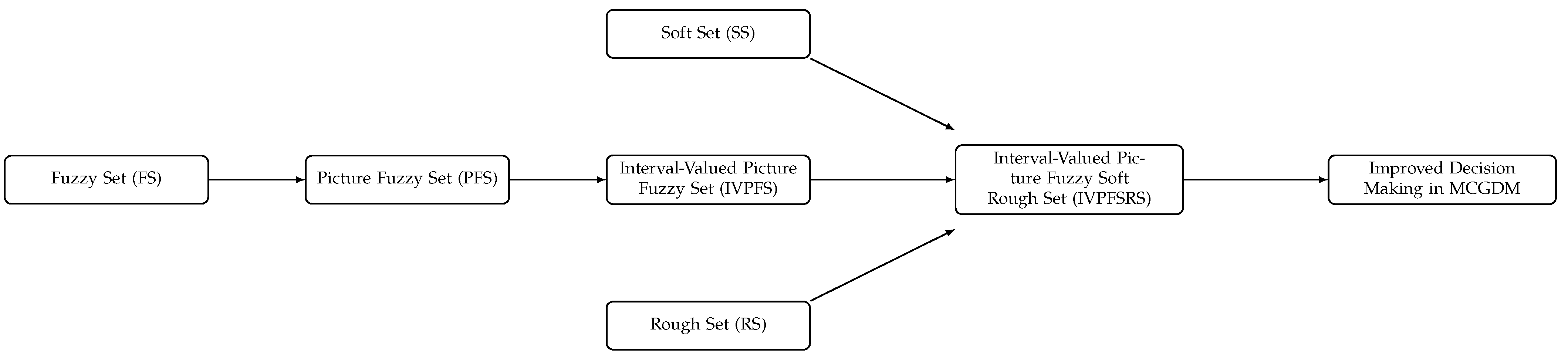
This section introduces the interval-valued picture fuzzy soft rough sets (IVPFSRS) by synergistically integrating interval-valued picture fuzzy soft sets (IVPFSS) with rough set (RS) theory, establishing fundamental properties and operations for the approximation operators. While recent cloud-rough integration models [34,35] have advanced large group decision making in linguistic environments, our IVPFSRS framework addresses distinct challenges: parameterized evaluation in structured decision problems and comprehensive uncertainty representation across three membership dimensions (positive, neutral, negative). The conceptual integration of fuzzy, soft, and rough theories is schematically illustrated in Figure 1, which presents the structural architecture of the proposed IVPFSRS framework.

Definition 11.

Consider a universal set ξ and a parameter set Γ. Consider an IVPFSS relation $\Phi \in IVPFSS(\xi \times \Gamma )$. The structure $(\xi ,\Gamma ,\Phi )$ forms an IVPF rough approximation space. For a given $ð\in IVPF(\Gamma )$ with membership function ${\mu }_{ð}$, neutral function $h_{ð}$, and nonmembership function ${\Psi }_{ð}$, we define the upper and lower IVPFS approximations as follows:

$$\begin{array}{cc}\hfill \overline{\Phi }\left(ð\right)& =\left\{〈\wp ,[{\mu }_{\overline{\Phi }\left(ð\right)}^L(\wp ),{\mu }_{\overline{\Phi }\left(ð\right)}^U(\wp )],[h_{\overline{\Phi }\left(ð\right)}^L(\wp ),h_{\overline{\Phi }\left(ð\right)}^U(\wp )],[{\Psi }_{\overline{\Phi }\left(ð\right)}^L(\wp ),{\Psi }_{\overline{\Phi }\left(ð\right)}^U(\wp )]〉\mid \wp \in \xi \right\}\hfill \end{array}$$

(24)

$$\begin{array}{cc}\hfill \underset{¯}{\Phi }\left(ð\right)& =\left\{〈\wp ,[{\mu }_{\underset{¯}{\Phi }\left(ð\right)}^L(\wp ),{\mu }_{\underset{¯}{\Phi }\left(ð\right)}^U(\wp )],[h_{\underset{¯}{\Phi }\left(ð\right)}^L(\wp ),h_{\underset{¯}{\Phi }\left(ð\right)}^U(\wp )],[{\Psi }_{\underset{¯}{\Phi }\left(ð\right)}^L(\wp ),{\Psi }_{\underset{¯}{\Phi }\left(ð\right)}^U(\wp )]〉\mid \wp \in \xi \right\}\hfill \end{array}$$

(25)

where the interval-valued membership degrees are calculated as:

$${\mu }_{\overline{\Phi }\left(ð\right)}^L(\wp )=\underset{\iota \in \Gamma }{\bigvee }\left[{\mu }_{\Phi }^L(\wp ,\iota )\wedge {\mu }_{ð}^L\left(\iota \right)\right]$$

$${\mu }_{\overline{\Phi }\left(ð\right)}^U(\wp )=\underset{\iota \in \Gamma }{\bigvee }\left[{\mu }_{\Phi }^U(\wp ,\iota )\wedge {\mu }_{ð}^U\left(\iota \right)\right]$$

$$h_{\overline{\Phi }\left(ð\right)}^L(\wp )=\underset{\iota \in \Gamma }{\bigwedge }\left[h_{\Phi }^L(\wp ,\iota )\vee h_{ð}^L\left(\iota \right)\right]$$

$$h_{\overline{\Phi }\left(ð\right)}^U(\wp )=\underset{\iota \in \Gamma }{\bigwedge }\left[h_{\Phi }^U(\wp ,\iota )\vee h_{ð}^U\left(\iota \right)\right]$$

$${\Psi }_{\overline{\Phi }\left(ð\right)}^L(\wp )=\underset{\iota \in \Gamma }{\bigwedge }\left[{\Psi }_{\Phi }^L(\wp ,\iota )\vee {\Psi }_{ð}^L\left(\iota \right)\right]$$

$${\Psi }_{\overline{\Phi }\left(ð\right)}^U(\wp )=\underset{\iota \in \Gamma }{\bigwedge }\left[{\Psi }_{\Phi }^U(\wp ,\iota )\vee {\Psi }_{ð}^U\left(\iota \right)\right]$$

$${\mu }_{\underset{¯}{\Phi }\left(ð\right)}^L(\wp )=\underset{\iota \in \Gamma }{\bigwedge }\left[{\mu }_{\Phi }^L(\wp ,\iota )\vee {\mu }_{ð}^L\left(\iota \right)\right]$$

$${\mu }_{\underset{¯}{\Phi }\left(ð\right)}^U(\wp )=\underset{\iota \in \Gamma }{\bigwedge }\left[{\mu }_{\Phi }^U(\wp ,\iota )\vee {\mu }_{ð}^U\left(\iota \right)\right]$$

$$h_{\underset{¯}{\Phi }\left(ð\right)}^L(\wp )=\underset{\iota \in \Gamma }{\bigwedge }\left[h_{\Phi }^L(\wp ,\iota )\vee h_{ð}^L\left(\iota \right)\right]$$

$$h_{\underset{¯}{\Phi }\left(ð\right)}^U(\wp )=\underset{\iota \in \Gamma }{\bigwedge }\left[h_{\Phi }^U(\wp ,\iota )\vee h_{ð}^U\left(\iota \right)\right]$$

$${\Psi }_{\underset{¯}{\Phi }\left(ð\right)}^L(\wp )=\underset{\iota \in \Gamma }{\bigvee }\left[{\Psi }_{\Phi }^L(\wp ,\iota )\wedge {\Psi }_{ð}^L\left(\iota \right)\right]$$

$${\Psi }_{\underset{¯}{\Phi }\left(ð\right)}^U(\wp )=\underset{\iota \in \Gamma }{\bigvee }\left[{\Psi }_{\Phi }^U(\wp ,\iota )\wedge {\Psi }_{ð}^U\left(\iota \right)\right]$$

and they satisfy:

$$\begin{array}{cc}\hfill 0& \le \left[{\mu }_{\overline{\Phi }\left(ð\right)}^U(\wp )+h_{\overline{\Phi }\left(ð\right)}^U(\wp )+{\Psi }_{\overline{\Phi }\left(ð\right)}^U(\wp )\right]\le 1,\hfill \\ \hfill 0& \le \left[{\mu }_{\underset{¯}{\Phi }\left(ð\right)}^U(\wp )+h_{\underset{¯}{\Phi }\left(ð\right)}^U(\wp )+{\Psi }_{\underset{¯}{\Phi }\left(ð\right)}^U(\wp )\right]\le 1\hfill \end{array}$$

(26)

where $\underset{¯}{\Phi }\left(ð\right)$ and $\overline{\Phi }\left(ð\right)$ are known as the lower and upper soft rough approximation mappings corresponding to interval-valued picture fuzzy sets. When $\underset{¯}{\Phi }\left(ð\right)=\overline{\Phi }\left(ð\right)$, the set ð is definable; if not, it is termed an IVPFS rough set. We denote by $\left(\underset{¯}{\Phi }\left(ð\right),\overline{\Phi }\left(ð\right)\right)$ an (IVPFS) soft rough set.

Remark 1.

Consider the triplet $(\xi ,\Gamma ,\Phi )$ and let $ð\in IVIF(\Gamma )$; we define $\overline{\Phi }\left(ð\right)$ and $\underset{¯}{\Phi }\left(ð\right)$ as follows:

$$\begin{array}{cc}\hfill \overline{\Phi }\left(ð\right)& =\left\{〈\wp ,\left[{\mu }_{\overline{\Phi }\left(ð\right)}^L(\wp ),{\mu }_{\overline{\Phi }\left(ð\right)}^U(\wp )\right],\left[{\Psi }_{\overline{\Phi }\left(ð\right)}^L(\wp ),{\Psi }_{\overline{\Phi }\left(ð\right)}^U(\wp )\right]〉\mid \wp \in \xi \right\},\hfill \\ \hfill \underset{¯}{\Phi }\left(ð\right)& =\left\{〈\wp ,\left[{\mu }_{\underset{¯}{\Phi }\left(ð\right)}^L(\wp ),{\mu }_{\underset{¯}{\Phi }\left(ð\right)}^U(\wp )\right],\left[{\Psi }_{\underset{¯}{\Phi }\left(ð\right)}^L(\wp ),{\Psi }_{\underset{¯}{\Phi }\left(ð\right)}^U(\wp )\right]〉\mid \wp \in \xi \right\}\hfill \end{array}$$

where

$$\begin{array}{cc}\hfill {\mu }_{\overline{\Phi }\left(ð\right)}^L(\wp )& =\underset{\iota \in \Gamma }{\bigvee }\left({\mu }_{\Phi }^L(\wp ,\iota )\wedge {\mu }_{ð}^L\left(\iota \right)\right),\hfill \\ \hfill {\mu }_{\overline{\Phi }\left(ð\right)}^U(\wp )& =\underset{\iota \in \Gamma }{\bigvee }\left({\mu }_{\Phi }^U(\wp ,\iota )\wedge {\mu }_{ð}^U\left(\iota \right)\right),\hfill \\ \hfill {\Psi }_{\overline{\Phi }\left(ð\right)}^L(\wp )& =\underset{\iota \in \Gamma }{\bigwedge }\left({\Psi }_{\Phi }^L(\wp ,\iota )\vee {\Psi }_{ð}^L\left(\iota \right)\right),\hfill \\ \hfill {\Psi }_{\overline{\Phi }\left(ð\right)}^U(\wp )& =\underset{\iota \in \Gamma }{\bigwedge }\left({\Psi }_{\Phi }^U(\wp ,\iota )\vee {\Psi }_{ð}^U\left(\iota \right)\right),\hfill \\ \hfill {\mu }_{\underset{¯}{\Phi }\left(ð\right)}^L(\wp )& =\underset{\iota \in \Gamma }{\bigwedge }\left({\mu }_{\Phi }^L(\wp ,\iota )\vee {\mu }_{ð}^L\left(\iota \right)\right),\hfill \\ \hfill {\mu }_{\underset{¯}{\Phi }\left(ð\right)}^U(\wp )& =\underset{\iota \in \Gamma }{\bigwedge }\left({\mu }_{\Phi }^U(\wp ,\iota )\vee {\mu }_{ð}^U\left(\iota \right)\right),\hfill \\ \hfill {\Psi }_{\underset{¯}{\Phi }\left(ð\right)}^L(\wp )& =\underset{\iota \in \Gamma }{\bigvee }\left({\Psi }_{\Phi }^L(\wp ,\iota )\wedge {\Psi }_{ð}^L\left(\iota \right)\right),\hfill \\ \hfill {\Psi }_{\underset{¯}{\Phi }\left(ð\right)}^U(\wp )& =\underset{\iota \in \Gamma }{\bigvee }\left({\Psi }_{\Phi }^U(\wp ,\iota )\wedge {\Psi }_{ð}^U\left(\iota \right)\right)\hfill \end{array}$$

and they have the terms:

$$\begin{array}{cc}\hfill 0& \le \left[{\mu }_{\overline{\Phi }\left(ð\right)}^U(\wp )+{\Psi }_{\overline{\Phi }\left(ð\right)}^U(\wp )\right]\le 1,\hfill \\ \hfill 0& \le \left[{\mu }_{\underset{¯}{\Phi }\left(ð\right)}^U(\wp )+{\Psi }_{\underset{¯}{\Phi }\left(ð\right)}^U(\wp )\right]\le 1\hfill \end{array}$$

ð is said to be definable if $\underset{¯}{\Phi }\left(ð\right)=\overline{\Phi }\left(ð\right)$. If not, it is called an (IVI) soft rough set.

Remark 2.

Consider the triplet $(\xi ,\Gamma ,\Phi )$ and let $ð\in IVPyF(\Gamma )$; we define $\overline{\Phi }\left(ð\right)$ and $\underset{¯}{\Phi }\left(ð\right)$ as in the above remark, where the interval-valued membership degrees have the following conditions:

$$\begin{array}{cc}\hfill 0& \le \left[{\left({\mu }_{\overline{\Phi }\left(ð\right)}^U(\wp )\right)}^2+{\left({\Psi }_{\overline{\Phi }\left(ð\right)}^U(\wp )\right)}^2\right]\le 1,\hfill \\ \hfill 0& \le \left[{\left({\mu }_{\underset{¯}{\Phi }\left(ð\right)}^U(\wp )\right)}^2+{\left({\Psi }_{\underset{¯}{\Phi }\left(ð\right)}^U(\wp )\right)}^2\right]\le 1\hfill \end{array}$$

under this condition ð is said to be definable if $\underset{¯}{\Phi }\left(ð\right)=\overline{\Phi }\left(ð\right)$. If not, it is called an IVPyF soft rough set.

Example 1.

Consider a scenario where a decision maker is evaluating four different cars, represented by the set $\xi =\{{\wp }_1,{\wp }_2,{\wp }_3,{\wp }_4\}$. Assume the parameter set $\Gamma =\{{\iota }_1,{\iota }_2,{\iota }_3\}=\{\mathit{expensive},\mathit{stylish},\mathit{\text{fuel-efficient}}\}$. Let us define $(\xi ,\Gamma ,\Phi )$ as an IVPFSS approximation space with $\Phi \in \mathit{IVPFSS}(\xi \times \Gamma )$ presented in

Table 2. Interval-valued picture fuzzy soft set (IVPFSS) relation $\Phi$ for car evaluation example.

$\mathbf{\Phi }$	${\mathit{\iota }}_1$	${\mathit{\iota }}_2$	${\mathit{\iota }}_3$
${\wp }_1$	$\left([0.10,0.25],[0.30,0.35],[0.20,0.40]\right)$	$\left([0.30,0.35],[0.25,0.45],[0.05,0.10]\right)$	$\left([0.20,0.30],[0.50,0.60],[0.05,0.10]\right)$
${\wp }_2$	$\left([0.10,0.20],[0.30,0.45],[0.15,0.25]\right)$	$\left([0.15,0.20],[0.30,0.50],[0.15,0.25]\right)$	$\left([0.25,0.40],[0.20,0.30],[0.10,0.20]\right)$
${\wp }_3$	$\left([0.15,0.25],[0.30,0.55],[0.05,0.15]\right)$	$\left([0.50,0.55],[0.10,0.15],[0.15,0.25]\right)$	$\left([0.40,0.50],[0.10,0.15],[0.10,0.25]\right)$
${\wp }_4$	$\left([0.50,0.55],[0.10,0.20],[0.15,0.20]\right)$	$\left([0.10,0.15],[0.30,0.40],[0.30,0.40]\right)$	$\left([0.40,0.55],[0.05,0.10],[0.20,0.35]\right)$

.

The table represents the IVPFSS relation Φ from four cars (${\wp }_1$–${\wp }_4$) to three criteria of evaluation. Each cell is filled with interval-valued membership, neutrality, and non-membership degrees that reflect expert opinions.

Now, consider the ideal decision object ð, as determined by the decision maker, is given by:

$$ð=\left\{\begin{array}{cc}& \langle {\iota }_1\left([0.4,0.55],[0.10,0.35],[0.50,0.10]\right)\rangle ,\hfill \\ & \langle {\iota }_2\left([0.20,0.30],[0.10,0.15],[0.30,0.45]\right)\rangle ,\hfill \\ & \langle {\iota }_3\left([0.40,0.60],[0.05,0.10],[0.15,0.20]\right)\rangle \hfill \end{array}\right\}$$

We have

$$\begin{array}{cc}\hfill {\mu }_{\overline{\Phi }\left(ð\right)}^L\left({\wp }_1\right)& =(0.10\wedge 0.40)\vee (0.30\wedge 0.20)\vee (0.20\wedge 0.40)=0.20\hfill \\ \hfill {\mu }_{\overline{\Phi }\left(ð\right)}^U\left({\wp }_1\right)& =(0.25\wedge 0.55)\vee (0.35\wedge 0.30)\vee (0.30\wedge 0.60)=0.30\hfill \\ \hfill h_{\overline{\Phi }\left(ð\right)}^L\left({\wp }_1\right)& =(0.30\vee 0.10)\wedge (0.25\vee 0.10)\wedge (0.50\vee 0.05)=0.25\hfill \\ \hfill h_{\overline{\Phi }\left(ð\right)}^U\left({\wp }_1\right)& =(0.35\vee 0.35)\wedge (0.45\vee 0.15)\wedge (0.60\vee 0.10)=0.35\hfill \\ \hfill {\Psi }_{\overline{\Phi }\left(ð\right)}^L\left({\wp }_1\right)& =(0.20\vee 0.05)\wedge (0.05\vee 0.30)\wedge (0.05\vee 0.15)=0.15\hfill \\ \hfill {\Psi }_{\overline{\Phi }\left(ð\right)}^U\left({\wp }_1\right)& =(0.40\vee 0.10)\wedge (0.10\vee 0.45)\wedge (0.10\vee 0.20)=0.20\hfill \end{array}$$

$$\begin{array}{cc}\hfill & \begin{array}{cccccccc}\hfill {\mu }_{\underset{¯}{\Phi }\left(ð\right)}^L\left({\wp }_1\right)& =0.30,\hfill & \hfill {\mu }_{\underset{¯}{\Phi }\left(ð\right)}^U\left({\wp }_1\right)& =0.35,\hfill & \hfill h_{\underset{¯}{\Phi }\left(ð\right)}^L\left({\wp }_1\right)& =0.25,\hfill & \hfill h_{\underset{¯}{\Phi }\left(ð\right)}^U\left({\wp }_1\right)& =0.35,\hfill \\ \hfill {\Psi }_{\underset{¯}{\Phi }\left(ð\right)}^L\left({\wp }_1\right)& =0.05,\hfill & \hfill {\Psi }_{\underset{¯}{\Phi }\left(ð\right)}^U\left({\wp }_1\right)& =0.10\hfill \end{array}\hfill \\ \hfill & \begin{array}{cccccccc}\hfill {\mu }_{\overline{\Phi }\left(ð\right)}^L\left({\wp }_2\right)& =0.25,\hfill & \hfill {\mu }_{\overline{\Phi }\left(ð\right)}^U\left({\wp }_2\right)& =0.40,\hfill & \hfill h_{\overline{\Phi }\left(ð\right)}^L\left({\wp }_2\right)& =0.30,\hfill & \hfill h_{\overline{\Phi }\left(ð\right)}^U\left({\wp }_2\right)& =0.30,\hfill \\ \hfill {\Psi }_{\overline{\Phi }\left(ð\right)}^L\left({\wp }_2\right)& =0.15,\hfill & \hfill {\Psi }_{\overline{\Phi }\left(ð\right)}^U\left({\wp }_2\right)& =0.20\hfill \end{array}\hfill \\ \hfill & \begin{array}{cccccccc}\hfill {\mu }_{\underset{¯}{\Phi }\left(ð\right)}^L\left({\wp }_2\right)& =0.20,\hfill & \hfill {\mu }_{\underset{¯}{\Phi }\left(ð\right)}^U\left({\wp }_2\right)& =0.30,\hfill & \hfill h_{\underset{¯}{\Phi }\left(ð\right)}^L\left({\wp }_2\right)& =0.30,\hfill & \hfill h_{\underset{¯}{\Phi }\left(ð\right)}^U\left({\wp }_2\right)& =0.30,\hfill \\ \hfill {\Psi }_{\underset{¯}{\Phi }\left(ð\right)}^L\left({\wp }_2\right)& =0.15,\hfill & \hfill {\Psi }_{\underset{¯}{\Phi }\left(ð\right)}^U\left({\wp }_2\right)& =0.25\hfill \end{array}\hfill \\ \hfill & \begin{array}{cccccccc}\hfill {\mu }_{\overline{\Phi }\left(ð\right)}^L\left({\wp }_3\right)& =0.40,\hfill & \hfill {\mu }_{\overline{\Phi }\left(ð\right)}^U\left({\wp }_3\right)& =0.50,\hfill & \hfill h_{\overline{\Phi }\left(ð\right)}^L\left({\wp }_3\right)& =0.10,\hfill & \hfill h_{\overline{\Phi }\left(ð\right)}^U\left({\wp }_3\right)& =0.15,\hfill \\ \hfill {\Psi }_{\overline{\Phi }\left(ð\right)}^L\left({\wp }_3\right)& =0.05,\hfill & \hfill {\Psi }_{\underset{¯}{\Phi }\left(ð\right)}^U\left({\wp }_3\right)& =0.15\hfill \end{array}\hfill \\ \hfill & \begin{array}{cccccccc}\hfill {\mu }_{\underset{¯}{\Phi }\left(ð\right)}^L\left({\wp }_3\right)& =0.40,\hfill & \hfill {\mu }_{\underset{¯}{\Phi }\left(ð\right)}^U\left({\wp }_3\right)& =0.55,\hfill & \hfill h_{\underset{¯}{\Phi }\left(ð\right)}^L\left({\wp }_3\right)& =0.10,\hfill & \hfill h_{\underset{¯}{\Phi }\left(ð\right)}^U\left({\wp }_3\right)& =0.15,\hfill \\ \hfill {\Psi }_{\underset{¯}{\Phi }\left(ð\right)}^L\left({\wp }_3\right)& =0.15,\hfill & \hfill {\Psi }_{\underset{¯}{\Phi }\left(ð\right)}^U\left({\wp }_3\right)& =0.25\hfill \end{array}\hfill \\ \hfill & \begin{array}{cccccccc}\hfill {\mu }_{\overline{\Phi }\left(ð\right)}^L\left({\wp }_4\right)& =0.40,\hfill & \hfill {\mu }_{\overline{\Phi }\left(ð\right)}^U\left({\wp }_4\right)& =0.55,\hfill & \hfill h_{\overline{\Phi }\left(ð\right)}^L\left({\wp }_4\right)& =0.05,\hfill & \hfill h_{\overline{\Phi }\left(ð\right)}^U\left({\wp }_4\right)& =0.10,\hfill \\ \hfill {\Psi }_{\overline{\Phi }\left(ð\right)}^L\left({\wp }_4\right)& =0.15,\hfill & \hfill {\Psi }_{\overline{\Phi }\left(ð\right)}^U\left({\wp }_4\right)& =0.20\hfill \end{array}\hfill \\ \hfill & \begin{array}{cccccccc}\hfill {\mu }_{\underset{¯}{\Phi }\left(ð\right)}^L\left({\wp }_4\right)& =0.20,\hfill & \hfill {\mu }_{\underset{¯}{\Phi }\left(ð\right)}^U\left({\wp }_4\right)& =0.30,\hfill & \hfill h_{\underset{¯}{\Phi }\left(ð\right)}^L\left({\wp }_4\right)& =0.05,\hfill & \hfill h_{\underset{¯}{\Phi }\left(ð\right)}^U\left({\wp }_4\right)& =0.10,\hfill \\ \hfill {\Psi }_{\underset{¯}{\Phi }\left(ð\right)}^L\left({\wp }_4\right)& =0.30,\hfill & \hfill {\Psi }_{\underset{¯}{\Phi }\left(ð\right)}^U\left({\wp }_4\right)& =0.40\hfill \end{array}\hfill \end{array}$$

Table 3. Interval-valued picture fuzzy soft rough approximation $\overline{\Phi }\left(ð\right)$.

$\overline{\mathbf{\Phi }}\left(\mathit{ð}\right)$	$[{\mathit{\mu }}_{\overline{\mathbf{\Phi }}\left(\mathit{ð}\right)}^{\mathit{L}}\left(\mathit{\wp }\right),{\mathit{\mu }}_{\overline{\mathbf{\Phi }}\left(\mathit{ð}\right)}^{\mathit{U}}\mathbf{\left(}\mathit{\wp }\right)]$	$[{\mathit{h}}_{\overline{\mathbf{\Phi }}\left(\mathit{ð}\right)}^{\mathit{L}}\left(\mathit{\wp }\right),{\mathit{h}}_{\overline{\mathbf{\Phi }}\left(\mathit{ð}\right)}^{\mathit{U}}\left(\mathit{\wp }\right)]$	$[{\mathbf{\Psi }}_{\overline{\mathbf{\Phi }}\left(\mathit{ð}\right)}^{\mathit{L}}\left(\mathit{\wp }\right),{\mathbf{\Psi }}_{\overline{\mathbf{\Phi }}\left(\mathit{ð}\right)}^{\mathit{U}}\left(\mathit{\wp }\right)]$
${\wp }_1$	[0.20, 0.30]	[0.25, 0.35]	[0.15, 0.20]
${\wp }_2$	[0.25, 0.40]	[0.30, 0.30]	[0.15, 0.20]
${\wp }_3$	[0.40, 0.50]	[0.10, 0.15]	[0.05, 0.15]
${\wp }_4$	[0.40, 0.55]	[0.05, 0.10]	[0.15, 0.20]

below illustrates the calculated interval-valued picture fuzzy soft rough approximations $\overline{\Phi }\left(\tilde{A}\right)$ for each alternative, obtained based on the defined IVPFSS relations.

Table 4. Interval-valued picture fuzzy soft rough approximation $\underset{¯}{\Phi }\left(ð\right)$.

$\underset{¯}{\mathbf{\Phi }}\left(\mathit{ð}\right)$	$[{\mathit{\mu }}_{\underset{¯}{\mathbf{\Phi }}\left(\mathit{ð}\right)}^{\mathit{L}}\left(\mathit{\wp }\right),{\mathit{\mu }}_{\underset{¯}{\mathbf{\Phi }}\left(\mathit{ð}\right)}^{\mathit{U}}\left(\mathit{\wp }\right)]$	$[{\mathit{h}}_{\underset{¯}{\mathbf{\Phi }}\left(\mathit{ð}\right)}^{\mathit{L}}\left(\mathit{\wp }\right),{\mathit{h}}_{\underset{¯}{\mathbf{\Phi }}\left(\mathit{ð}\right)}^{\mathit{U}}\left(\mathit{\wp }\right)]$	$[{\mathbf{\Psi }}_{\underset{¯}{\mathbf{\Phi }}\left(\mathit{ð}\right)}^{\mathit{L}}\left(\mathit{\wp }\right),{\mathbf{\Psi }}_{\underset{¯}{\mathbf{\Phi }}\left(\mathit{ð}\right)}^{\mathit{U}}\left(\mathit{\wp }\right)]$
${\wp }_1$	[0.30, 0.35]	[0.25, 0.35]	[0.05, 0.10]
${\wp }_2$	[0.20, 0.30]	[0.30, 0.30]	[0.15, 0.25]
${\wp }_3$	[0.40, 0.55]	[0.10, 0.15]	[0.15, 0.25]
${\wp }_4$	[0.20, 0.30]	[0.05, 0.10]	[0.30, 0.40]

below shows the corresponding interval-valued picture fuzzy soft rough approximations $\Phi \left(\tilde{A}\right)$, providing the upper bounds of uncertainty for each evaluated alternative.

Definition 12.

Assume that $\underset{¯}{\Phi }\left(ð\right)$ and $\overline{\Phi }\left(ð\right)$ represent the lower and the upper soft rough approximations over interval-valued picture fuzzy sets. We define the following algebraic operations:

i. 

Algebraic sum operation (⊕):

$$\begin{array}{cc}\hfill \overline{\Phi }\left(ð\right)\oplus \underset{¯}{\Phi }\left(ð\right)=\{\langle \wp ,& [1-(1-{\mu }_{\overline{\Phi }\left(ð\right)}^L(\wp ))(1-{\mu }_{\underset{¯}{\Phi }\left(ð\right)}^L(\wp )),\hfill \\ \hfill & 1-(1-{\mu }_{\overline{\Phi }\left(ð\right)}^U(\wp ))(1-{\mu }_{\underset{¯}{\Phi }\left(ð\right)}^U(\wp ))],\hfill \\ \hfill & \left[h_{\overline{\Phi }\left(ð\right)}^L(\wp )h_{\underset{¯}{\Phi }\left(ð\right)}^L(\wp ),h_{\overline{\Phi }\left(ð\right)}^U(\wp )h_{\underset{¯}{\Phi }\left(ð\right)}^U(\wp )\right],\hfill \\ \hfill & \left[{\Psi }_{\overline{\Phi }\left(ð\right)}^L(\wp ){\Psi }_{\underset{¯}{\Phi }\left(ð\right)}^L(\wp ),{\Psi }_{\overline{\Phi }\left(ð\right)}^U(\wp ){\Psi }_{\underset{¯}{\Phi }\left(ð\right)}^U(\wp )\right]\rangle \mid \wp \in \xi \}\hfill \end{array}$$

(27)

ii. 

Algebraic product operation (⊗):

$$\begin{array}{cc}\hfill \overline{\Phi }\left(ð\right)\otimes \underset{¯}{\Phi }\left(ð\right)=\{\langle \wp ,& \left[{\mu }_{\overline{\Phi }\left(ð\right)}^L(\wp ){\mu }_{\underset{¯}{\Phi }\left(ð\right)}^L(\wp ),{\mu }_{\overline{\Phi }\left(ð\right)}^U(\wp ){\mu }_{\underset{¯}{\Phi }\left(ð\right)}^U(\wp )\right],\hfill \\ \hfill & [1-(1-h_{\overline{\Phi }\left(ð\right)}^L(\wp ))(1-h_{\underset{¯}{\Phi }\left(ð\right)}^L(\wp )),\hfill \\ \hfill & 1-(1-h_{\overline{\Phi }\left(ð\right)}^U(\wp ))(1-h_{\underset{¯}{\Phi }\left(ð\right)}^U(\wp ))],\hfill \\ \hfill & [1-(1-{\Psi }_{\overline{\Phi }\left(ð\right)}^L(\wp ))(1-{\Psi }_{\underset{¯}{\Phi }\left(ð\right)}^L(\wp )),\hfill \\ \hfill & 1-(1-{\Psi }_{\overline{\Phi }\left(ð\right)}^U(\wp ))(1-{\Psi }_{\underset{¯}{\Phi }\left(ð\right)}^U(\wp ))]\rangle \mid \wp \in \xi \}\hfill \end{array}$$

(28)

Table 5. Results of algebraic sum operation $\overline{\Phi }\left(ð\right)\oplus \underset{¯}{\Phi }\left(ð\right)$ for car selection example.

$\overline{\mathbf{\Phi }}\left(\mathit{ð}\right)\oplus \underset{¯}{\mathbf{\Phi }}\left(\mathit{ð}\right)$	$\begin{array}{c}\hfill [1-(1-{\mathit{\mu }}_{\overline{\mathbf{\Phi }}\left(\mathit{ð}\right)}^{\mathit{L}}\left(\mathit{\wp }\right))(1-{\mathit{\mu }}_{\underset{¯}{\mathbf{\Phi }}\left(\mathit{ð}\right)}^{\mathit{L}}\left(\mathit{\wp }\right)),\\ \hfill 1-(1-{\mathit{\mu }}_{\overline{\mathbf{\Phi }}\left(\mathit{ð}\right)}^{\mathit{U}}\left(\mathit{\wp }\right))(1-{\mathit{\mu }}_{\underset{¯}{\mathbf{\Phi }}\left(\mathit{ð}\right)}^{\mathit{U}}\left(\mathit{\wp }\right))]\end{array}$	$\begin{array}{c}\hfill [{\mathit{h}}_{\overline{\mathbf{\Phi }}\left(\mathit{ð}\right)}^{\mathit{L}}\left(\mathit{\wp }\right){\mathit{h}}_{\underset{¯}{\mathbf{\Phi }}\left(\mathit{ð}\right)}^{\mathit{L}}\left(\mathit{\wp }\right),\\ \hfill {\mathit{h}}_{\overline{\mathbf{\Phi }}\left(\mathit{ð}\right)}^{\mathit{U}}\left(\mathit{\wp }\right){\mathit{h}}_{\underset{¯}{\mathbf{\Phi }}\left(\mathit{ð}\right)}^{\mathit{U}}\left(\mathit{\wp }\right)]\end{array}$	$\begin{array}{c}\hfill [1-(1-{\mathbf{\Psi }}_{\overline{\mathbf{\Phi }}\left(\mathit{ð}\right)}^{\mathit{L}}\left(\mathit{\wp }\right))(1-{\mathbf{\Psi }}_{\underset{¯}{\mathbf{\Phi }}\left(\mathit{ð}\right)}^{\mathit{L}}\left(\mathit{\wp }\right)),\\ \hfill 1-(1-{\mathbf{\Psi }}_{\overline{\mathbf{\Phi }}\left(\mathit{ð}\right)}^{\mathit{U}}\left(\mathit{\wp }\right))(1-{\mathbf{\Psi }}_{\underset{¯}{\mathbf{\Phi }}\left(\mathit{ð}\right)}^{\mathit{U}}\left(\mathit{\wp }\right))]\end{array}$
${\wp }_1$	[0.44, 0.54]	[0.06, 0.12]	[0.007, 0.02]
${\wp }_2$	[0.40, 0.58]	[0.09, 0.09]	[0.02, 0.05]
${\wp }_3$	[0.64, 0.77]	[0.01, 0.02]	[0.007, 0.03]
${\wp }_4$	[0.52, 0.68]	[0.002, 0.01]	[0.04, 0.08]

below presents the aggregated results of $\overline{\Phi }\left(\tilde{A}\right)\oplus \Phi \left(\tilde{A}\right)$, representing the combined upper and lower approximations through the defined fuzzy addition operation.

This table presents the aggregated results from combining upper and lower approximations using algebraic sum operation. The data corresponds to the car evaluation scenario in Table 2, with ð  representing the ideal car profile.

Therefore, ${\wp }_3$ is identified as the best choice, as it has the highest membership value at $0.77$ and the lowest non-membership value at $0.007$.

Table 6. Results of algebraic product operation $\overline{\Phi }\left(ð\right)\otimes \underset{¯}{\Phi }\left(ð\right)$ for car selection example.

$\overline{\mathbf{\Phi }}\left(\mathit{ð}\right)\otimes \underset{¯}{\mathbf{\Phi }}\left(\mathit{ð}\right)$	$\begin{array}{c}\hfill [{\mathit{\mu }}_{\overline{\mathbf{\Phi }}\left(\mathit{ð}\right)}^{\mathit{L}}\left(\mathit{\wp }\right){\mathit{\mu }}_{\underset{¯}{\mathbf{\Phi }}\left(\mathit{ð}\right)}^{\mathit{L}}\left(\mathit{\wp }\right),\\ \hfill {\mathit{\mu }}_{\overline{\mathbf{\Phi }}\left(\mathit{ð}\right)}^{\mathit{U}}\left(\mathit{\wp }\right){\mathit{\mu }}_{\underset{¯}{\mathbf{\Phi }}\left(\mathit{ð}\right)}^{\mathit{U}}\left(\mathit{\wp }\right)]\end{array}$	$\begin{array}{c}\hfill [1-(1-{\mathit{h}}_{\overline{\mathbf{\Phi }}\left(\mathit{ð}\right)}^{\mathit{L}}\left(\mathit{\wp }\right))(1-{\mathit{h}}_{\underset{¯}{\mathbf{\Phi }}\left(\mathit{ð}\right)}^{\mathit{L}}\left(\mathit{\wp }\right)),\\ \hfill 1-(1-{\mathit{h}}_{\overline{\mathbf{\Phi }}\left(\mathit{ð}\right)}^{\mathit{U}}\left(\mathit{\wp }\right))(1-{\mathit{h}}_{\underset{¯}{\mathbf{\Phi }}\left(\mathit{ð}\right)}^{\mathit{U}}\left(\mathit{\wp }\right))]\end{array}$	$\begin{array}{c}\hfill [1-(1-{\mathbf{\Psi }}_{\overline{\mathbf{\Phi }}\left(\mathit{ð}\right)}^{\mathit{L}}\left(\mathit{\wp }\right))(1-{\mathbf{\Psi }}_{\underset{¯}{\mathbf{\Phi }}\left(\mathit{ð}\right)}^{\mathit{L}}\left(\mathit{\wp }\right)),\\ \hfill 1-(1-{\mathbf{\Psi }}_{\overline{\mathbf{\Phi }}\left(\mathit{ð}\right)}^{\mathit{U}}\left(\mathit{\wp }\right))(1-{\mathbf{\Psi }}_{\underset{¯}{\mathbf{\Phi }}\left(\mathit{ð}\right)}^{\mathit{U}}\left(\mathit{\wp }\right))]\end{array}$
${\wp }_1$	[0.06, 0.10]	[0.43, 0.57]	[0.19, 0.28]
${\wp }_2$	[0.05, 0.12]	[0.51, 0.51]	[0.27, 0.40]
${\wp }_3$	[0.16, 0.27]	[0.19, 0.27]	[0.19, 0.36]
${\wp }_4$	[0.08, 0.16]	[0.09, 0.19]	[0.40, 0.52]

below displays the results of $\overline{\Phi }\left(\tilde{A}\right)\otimes \Phi \left(\tilde{A}\right)$, illustrating the intersection operation of the interval-valued picture fuzzy soft rough approximations and supporting the decision analysis.

This table presents the aggregated results from combining upper and lower approximations using algebraic product operation. The data corresponds to the car evaluation scenario in Table 2, with ð representing the ideal car profile.

We note that ${\wp }_3$ is still the ideal decision.

Hence, the decision maker will purchase car ${\wp }_3$.

Definition 13.

Let $\Phi \left(ð\right)=(\underset{¯}{\Phi }\left(ð\right),\overline{\Phi }\left(ð\right))$ be an IVPF soft rough number. We denote by $\sim \Phi \left(ð\right)=(\underset{¯}{\Phi }{\left(ð\right)}^c,\overline{\Phi }{\left(ð\right)}^c)$ the complement of the IVPF soft rough number, where $\underset{¯}{\Phi }{\left(ð\right)}^c$, $\overline{\Phi }{\left(ð\right)}^c$ are referred to as the complements of $\underset{¯}{\Phi }\left(ð\right)$ and $\overline{\Phi }\left(ð\right)$, respectively, and they are defined as follows:

$$\begin{array}{cc}\hfill \underset{¯}{\Phi }{\left(ð\right)}^c& =\left\{〈\wp ,[{\Psi }_{\underset{¯}{\Phi }\left(ð\right)}^L(\wp ),{\Psi }_{\underset{¯}{\Phi }\left(ð\right)}^U(\wp )],[h_{\underset{¯}{\Phi }\left(ð\right)}^L(\wp ),h_{\underset{¯}{\Phi }\left(ð\right)}^U(\wp )],[{\mu }_{\underset{¯}{\Phi }\left(ð\right)}^L(\wp ),{\mu }_{\underset{¯}{\Phi }\left(ð\right)}^U(\wp )]〉\mid \wp \in \xi \right\},\hfill \\ \hfill \overline{\Phi }{\left(ð\right)}^c& =\left\{〈\wp ,[{\Psi }_{\overline{\Phi }\left(ð\right)}^L(\wp ),{\Psi }_{\overline{\Phi }\left(ð\right)}^U(\wp )],[h_{\overline{\Phi }\left(ð\right)}^L(\wp ),h_{\overline{\Phi }\left(ð\right)}^U(\wp )],[{\mu }_{\overline{\Phi }\left(ð\right)}^L(\wp ),{\mu }_{\overline{\Phi }\left(ð\right)}^U(\wp )]〉\mid \wp \in \xi \right\}.\hfill \end{array}$$

Definition 14.

Consider two IVPF soft rough numbers $\Phi \left({ð}_1\right)$ and $\Phi \left({ð}_2\right)$. Then we define the following extended algebraic operations:

(i) 

Algebraic sum (⊕):

$$\begin{array}{cc}\hfill \Phi \left({ð}_1\right)\oplus \Phi \left({ð}_2\right)=& (\left(\left[{\mu }_{\underset{¯}{\Phi }\left({ð}_1\right)}^L+{\mu }_{\underset{¯}{\Phi }\left({ð}_2\right)}^L-{\mu }_{\underset{¯}{\Phi }\left({ð}_1\right)}^L{\mu }_{\underset{¯}{\Phi }\left({ð}_2\right)}^L,{\mu }_{\underset{¯}{\Phi }\left({ð}_1\right)}^U+{\mu }_{\underset{¯}{\Phi }\left({ð}_2\right)}^U-{\mu }_{\underset{¯}{\Phi }\left({ð}_1\right)}^U{\mu }_{\underset{¯}{\Phi }\left({ð}_2\right)}^U\right],\right.\hfill \\ \hfill & \left.\left[h_{\underset{¯}{\Phi }\left({ð}_1\right)}^L{h}_{\underset{¯}{\Phi }\left({ð}_2\right)}^L,h_{\underset{¯}{\Phi }\left({ð}_1\right)}^U{h}_{\underset{¯}{\Phi }\left({ð}_2\right)}^U\right],\left[{\Psi }_{\underset{¯}{\Phi }\left({ð}_1\right)}^L{\Psi }_{\underset{¯}{\Phi }\left({ð}_2\right)}^L,{\Psi }_{\underset{¯}{\Phi }\left({ð}_1\right)}^U{\Psi }_{\underset{¯}{\Phi }\left({ð}_2\right)}^U\right]\right),\hfill \\ \hfill & \left(\left[{\mu }_{\overline{\Phi }\left({ð}_1\right)}^L+{\mu }_{\overline{\Phi }\left({ð}_2\right)}^L-{\mu }_{\overline{\Phi }\left({ð}_1\right)}^L{\mu }_{\overline{\Phi }\left({ð}_2\right)}^L,{\mu }_{\overline{\Phi }\left({ð}_1\right)}^U+{\mu }_{\overline{\Phi }\left({ð}_2\right)}^U-{\mu }_{\overline{\Phi }\left({ð}_1\right)}^U{\mu }_{\overline{\Phi }\left({ð}_2\right)}^U\right],\right.\hfill \\ \hfill & \left.\left[h_{\overline{\Phi }\left({ð}_1\right)}^L{h}_{\overline{\Phi }\left({ð}_2\right)}^L,h_{\overline{\Phi }\left({ð}_1\right)}^U{h}_{\overline{\Phi }\left({ð}_2\right)}^U\right],\left[{\Psi }_{\overline{\Phi }\left({ð}_1\right)}^L{\Psi }_{\overline{\Phi }\left({ð}_2\right)}^L,{\Psi }_{\overline{\Phi }\left({ð}_1\right)}^U{\Psi }_{\overline{\Phi }\left({ð}_2\right)}^U\right]\right))\hfill \end{array}$$

(29)

(ii) 

Algebraic product (⊗):

$$\begin{array}{cc}\hfill \Phi \left({ð}_1\right)\otimes \Phi \left({ð}_2\right)=& (\left(\left[{\mu }_{\underset{¯}{\Phi }\left({ð}_1\right)}^L{\mu }_{\underset{¯}{\Phi }\left({ð}_2\right)}^L,{\mu }_{\underset{¯}{\Phi }\left({ð}_1\right)}^U{\mu }_{\underset{¯}{\Phi }\left({ð}_2\right)}^U\right],\right.\hfill \\ \hfill & \left[h_{\underset{¯}{\Phi }\left({ð}_1\right)}^L+h_{\underset{¯}{\Phi }\left({ð}_2\right)}^L-h_{\underset{¯}{\Phi }\left({ð}_1\right)}^L{h}_{\underset{¯}{\Phi }\left({ð}_2\right)}^L,h_{\underset{¯}{\Phi }\left({ð}_1\right)}^U+h_{\underset{¯}{\Phi }\left({ð}_2\right)}^U-h_{\underset{¯}{\Phi }\left({ð}_1\right)}^U{h}_{\underset{¯}{\Phi }\left({ð}_2\right)}^U\right],\hfill \\ \hfill & \left.\left[{\Psi }_{\underset{¯}{\Phi }\left({ð}_1\right)}^L+{\Psi }_{\underset{¯}{\Phi }\left({ð}_2\right)}^L-{\Psi }_{\underset{¯}{\Phi }\left({ð}_1\right)}^L{\Psi }_{\underset{¯}{\Phi }\left({ð}_2\right)}^L,{\Psi }_{\underset{¯}{\Phi }\left({ð}_1\right)}^U+{\Psi }_{\underset{¯}{\Phi }\left({ð}_2\right)}^U-{\Psi }_{\underset{¯}{\Phi }\left({ð}_1\right)}^U{\Psi }_{\underset{¯}{\Phi }\left({ð}_2\right)}^U\right]\right),\hfill \\ \hfill & \left(\left[{\mu }_{\overline{\Phi }\left({ð}_1\right)}^L{\mu }_{\overline{\Phi }\left({ð}_2\right)}^L,{\mu }_{\overline{\Phi }\left({ð}_1\right)}^U{\mu }_{\overline{\Phi }\left({ð}_2\right)}^U\right],\right.\hfill \\ \hfill & \left[h_{\overline{\Phi }\left({ð}_1\right)}^L+h_{\overline{\Phi }\left({ð}_2\right)}^L-h_{\overline{\Phi }\left({ð}_1\right)}^L{h}_{\overline{\Phi }\left({ð}_2\right)}^L,h_{\overline{\Phi }\left({ð}_1\right)}^U+h_{\overline{\Phi }\left({ð}_2\right)}^U-h_{\overline{\Phi }\left({ð}_1\right)}^U{h}_{\overline{\Phi }\left({ð}_2\right)}^U\right],\hfill \\ \hfill & \left.\left[{\Psi }_{\overline{\Phi }\left({ð}_1\right)}^L+{\Psi }_{\overline{\Phi }\left({ð}_2\right)}^L-{\Psi }_{\overline{\Phi }\left({ð}_1\right)}^L{\Psi }_{\overline{\Phi }\left({ð}_2\right)}^L,{\Psi }_{\overline{\Phi }\left({ð}_1\right)}^U+{\Psi }_{\overline{\Phi }\left({ð}_2\right)}^U-{\Psi }_{\overline{\Phi }\left({ð}_1\right)}^U{\Psi }_{\overline{\Phi }\left({ð}_2\right)}^U\right]\right))\hfill \end{array}$$

(30)

(iii) 

Scalar multiplication ($\widehat{o}\Phi \left({ð}_1\right)$):

$$\begin{array}{cc}\hfill \widehat{o}\Phi \left({ð}_1\right)=& (\left(\left[1-{(1-{\mu }_{\underset{¯}{\Phi }\left({ð}_1\right)}^L)}^{\widehat{o}},1-{(1-{\mu }_{\underset{¯}{\Phi }\left({ð}_1\right)}^U)}^{\widehat{o}}\right],\right.\hfill \\ \hfill & \left[{\left(h_{\underset{¯}{\Phi }\left({ð}_1\right)}^L\right)}^{\widehat{o}},{\left(h_{\underset{¯}{\Phi }\left({ð}_1\right)}^U\right)}^{\widehat{o}}\right],\left[{\left({\Psi }_{\underset{¯}{\Phi }\left({ð}_1\right)}^L\right)}^{\widehat{o}},{\left({\Psi }_{\underset{¯}{\Phi }\left({ð}_1\right)}^U\right)}^{\widehat{o}}\right]),\hfill \\ \hfill & (\left[1-{(1-{\mu }_{\overline{\Phi }\left({ð}_1\right)}^L)}^{\widehat{o}},1-{(1-{\mu }_{\overline{\Phi }\left({ð}_1\right)}^U)}^{\widehat{o}}\right],\hfill \\ \hfill & \left[{\left(h_{\overline{\Phi }\left({ð}_1\right)}^L\right)}^{\widehat{o}},{\left(h_{\overline{\Phi }\left({ð}_1\right)}^U\right)}^{\widehat{o}}\right],\left[{\left({\Psi }_{\overline{\Phi }\left({ð}_1\right)}^L\right)}^{\widehat{o}},{\left({\Psi }_{\overline{\Phi }\left({ð}_1\right)}^U\right)}^{\widehat{o}}\right]\left)\right),\widehat{o}>0.\hfill \end{array}$$

(31)

(iv) 

Power operation (${(\Phi \left({ð}_1\right))}^{\widehat{o}}$):

$$\begin{array}{cc}\hfill {\left(\Phi \left({ð}_1\right)\right)}^{\widehat{o}}=& (\left(\left[{\left({\mu }_{\underset{¯}{\Phi }\left({ð}_1\right)}^L\right)}^{\widehat{o}},{\left({\mu }_{\underset{¯}{\Phi }\left({ð}_1\right)}^U\right)}^{\widehat{o}}\right],\right.\left[1-{(1-h_{\underset{¯}{\Phi }\left({ð}_1\right)}^L)}^{\widehat{o}},1-{(1-h_{\underset{¯}{\Phi }\left({ð}_1\right)}^U)}^{\widehat{o}}\right],\hfill \\ \hfill & \left[1-{(1-{\Psi }_{\underset{¯}{\Phi }\left({ð}_1\right)}^L)}^{\widehat{o}},1-{(1-{\Psi }_{\underset{¯}{\Phi }\left({ð}_1\right)}^U)}^{\widehat{o}}\right]),\hfill \\ \hfill & (\left[{\left({\mu }_{\overline{\Phi }\left({ð}_1\right)}^L\right)}^{\widehat{o}},{\left({\mu }_{\overline{\Phi }\left({ð}_1\right)}^U\right)}^{\widehat{o}}\right],\left[1-{(1-h_{\overline{\Phi }\left({ð}_1\right)}^L)}^{\widehat{o}},1-{(1-h_{\overline{\Phi }\left({ð}_1\right)}^U)}^{\widehat{o}}\right],\hfill \\ \hfill & \left[1-{(1-{\Psi }_{\overline{\Phi }\left({ð}_1\right)}^L)}^{\widehat{o}},1-{(1-{\Psi }_{\overline{\Phi }\left({ð}_1\right)}^U)}^{\widehat{o}}\right]\left)\right),\widehat{o}>0.\hfill \end{array}$$

(32)

Example 2.

Let $\Phi \left({ð}_1\right)=(\underset{¯}{\Phi }\left({ð}_1\right),\overline{\Phi }\left({ð}_1\right))$ and $\Phi \left({ð}_2\right)=(\underset{¯}{\Phi }\left({ð}_2\right),\overline{\Phi }\left({ð}_2\right))$ where $\underset{¯}{\Phi }\left({ð}_1\right)$, $\overline{\Phi }\left({ð}_1\right)$, $\underset{¯}{\Phi }\left({ð}_2\right)$, $\overline{\Phi }\left({ð}_2\right)$ are given as below:

Table 7. $\underset{¯}{\Phi }\left({ð}_1\right)$.

$\underset{¯}{\mathbf{\Phi }}\left({\mathit{ð}}_1\right)$	$\left[{\mathit{\mu }}_{\underset{¯}{\mathbf{\Phi }}\left({\mathit{ð}}_1\right)}^{\mathit{L}}\left(\mathit{\wp }\right),{\mathit{\mu }}_{\underset{¯}{\mathbf{\Phi }}\left({\mathit{ð}}_1\right)}^{\mathit{U}}\left(\mathit{\wp }\right)\right]$	$\left[{\mathit{h}}_{\underset{¯}{\mathbf{\Phi }}\left({\mathit{ð}}_1\right)}^{\mathit{L}}\left(\mathit{\wp }\right),{\mathit{h}}_{\underset{¯}{\mathbf{\Phi }}\left({\mathit{ð}}_1\right)}^{\mathit{U}}\left(\mathit{\wp }\right)\right]$	$\left[{\mathbf{\Psi }}_{\underset{¯}{\mathbf{\Phi }}\left({\mathit{ð}}_1\right)}^{\mathit{L}}\left(\mathit{\wp }\right),{\mathbf{\Psi }}_{\underset{¯}{\mathbf{\Phi }}\left({\mathit{ð}}_1\right)}^{\mathit{U}}\left(\mathit{\wp }\right)\right]$
${\wp }_1$	[0.20, 0.30]	[0.10, 0.15]	[0.15, 0.20]
${\wp }_2$	[0.25, 0.30]	[0.20, 0.30]	[0.10, 0.20]
${\wp }_3$	[0.30, 0.40]	[0.15, 0.20]	[0.10, 0.15]

below contains the interval-valued picture fuzzy soft rough number $\Phi \left({\tilde{A}}_1\right)$, including the lower approximations for the corresponding alternatives.

Table 8. $\overline{\Phi }\left({ð}_1\right)$.

$\overline{\mathbf{\Phi }}\left({\mathit{ð}}_1\right)$	$\left[{\mathit{\mu }}_{\overline{\mathbf{\Phi }}\left({\mathit{ð}}_1\right)}^{\mathit{L}}\left(\mathit{\wp }\right),{\mathit{\mu }}_{\overline{\mathbf{\Phi }}\left({\mathit{ð}}_1\right)}^{\mathit{U}}\left(\mathit{\wp }\right)\right]$	$\left[{\mathit{h}}_{\overline{\mathbf{\Phi }}\left({\mathit{ð}}_1\right)}^{\mathit{L}}\left(\mathit{\wp }\right),{\mathit{h}}_{\overline{\mathbf{\Phi }}\left({\mathit{ð}}_1\right)}^{\mathit{U}}\left(\mathit{\wp }\right)\right]$	$\left[{\mathbf{\Psi }}_{\overline{\mathbf{\Phi }}\left({\mathit{ð}}_1\right)}^{\mathit{L}}\left(\mathit{\wp }\right),{\mathbf{\Psi }}_{\overline{\mathbf{\Phi }}\left({\mathit{ð}}_1\right)}^{\mathit{U}}\left(\mathit{\wp }\right)\right]$
${\wp }_1$	[0.25, 0.35]	[0.10, 0.15]	[0.15, 0.20]
${\wp }_2$	[0.20, 0.30]	[0.20, 0.30]	[0.15, 0.25]
${\wp }_3$	[0.35, 0.45]	[0.15, 0.20]	[0.15, 0.25]

below presents the upper approximations $\Phi \left({\tilde{A}}_1\right)$ associated with the same dataset as in Table 7, allowing for comparison of the corresponding uncertainty levels.

Table 9. $\underset{¯}{\Phi }\left({ð}_2\right)$.

$\underset{¯}{\mathbf{\Phi }}\left({\mathit{ð}}_2\right)$	$\left[{\mathit{\mu }}_{\underset{¯}{\mathbf{\Phi }}\left({\mathit{ð}}_2\right)}^{\mathit{L}}\left(\mathit{\wp }\right),{\mathit{\mu }}_{\underset{¯}{\mathbf{\Phi }}\left({\mathit{ð}}_2\right)}^{\mathit{U}}\left(\mathit{\wp }\right)\right]$	$\left[{\mathit{h}}_{\underset{¯}{\mathbf{\Phi }}\left({\mathit{ð}}_2\right)}^{\mathit{L}}\left(\mathit{\wp }\right),{\mathit{h}}_{\underset{¯}{\mathbf{\Phi }}\left({\mathit{ð}}_2\right)}^{\mathit{U}}\left(\mathit{\wp }\right)\right]$	$\left[{\mathbf{\Psi }}_{\underset{¯}{\mathbf{\Phi }}\left({\mathit{ð}}_2\right)}^{\mathit{L}}\left(\mathit{\wp }\right),{\mathbf{\Psi }}_{\underset{¯}{\mathbf{\Phi }}\left({\mathit{ð}}_2\right)}^{\mathit{U}}\left(\mathit{\wp }\right)\right]$
${\wp }_1$	[0.30, 0.40]	[0.15, 0.25]	[0.10, 0.15]
${\wp }_2$	[0.20, 0.30]	[0.10, 0.20]	[0.20, 0.30]
${\wp }_3$	[0.10, 0.25]	[0.20, 0.25]	[0.15, 0.20]

below provides the interval-valued picture fuzzy soft rough number $\Phi \left({\tilde{A}}_2\right)$, which defines the lower approximations for the second evaluated dataset.

Table 10. $\overline{\Phi }\left({ð}_2\right)$.

$\overline{\mathbf{\Phi }}\left({\mathit{ð}}_2\right)$	$\left[{\mathit{\mu }}_{\overline{\mathbf{\Phi }}\left({\mathit{ð}}_2\right)}^{\mathit{L}}\left(\mathit{\wp }\right),{\mathit{\mu }}_{\overline{\mathbf{\Phi }}\left({\mathit{ð}}_2\right)}^{\mathit{U}}\left(\mathit{\wp }\right)\right]$	$\left[{\mathit{h}}_{\overline{\mathbf{\Phi }}\left({\mathit{ð}}_2\right)}^{\mathit{L}}\left(\mathit{\wp }\right),{\mathit{h}}_{\overline{\mathbf{\Phi }}\left({\mathit{ð}}_2\right)}^{\mathit{U}}\left(\mathit{\wp }\right)\right]$	$\left[{\mathbf{\Psi }}_{\overline{\mathbf{\Phi }}\left({\mathit{ð}}_2\right)}^{\mathit{L}}\left(\mathit{\wp }\right),{\mathbf{\Psi }}_{\overline{\mathbf{\Phi }}\left({\mathit{ð}}_2\right)}^{\mathit{U}}\left(\mathit{\wp }\right)\right]$
${\wp }_1$	[0.30, 0.35]	[0.15, 0.25]	[0.15, 0.20]
${\wp }_2$	[0.30, 0.40]	[0.10, 0.20]	[0.25, 0.45]
${\wp }_3$	[0.25, 0.35]	[0.20, 0.25]	[0.15, 0.25]

below shows the upper approximations $\Phi \left({\tilde{A}}_2\right)$ corresponding to Table 9, facilitating comparative analysis between the two soft rough numbers.

Now we will calculate $\Phi \left({ð}_1\right)\oplus \Phi \left({ð}_2\right)$ and $\Phi \left({ð}_1\right)\otimes \Phi \left({ð}_2\right)$ based on the formulations given in Definition 14.

Table 11. $\underset{¯}{\Phi }\left({ð}_1\right)\oplus \underset{¯}{\Phi }\left({ð}_2\right)$.

$\underset{¯}{\mathbf{\Phi }}\left({\mathit{ð}}_1\right)\oplus \underset{¯}{\mathbf{\Phi }}\left({\mathit{ð}}_2\right)$	$\begin{array}{c}\hfill \left[{\mathit{\mu }}_{\underset{¯}{\mathbf{\Phi }}\left({\mathit{ð}}_1\right)}^{\mathit{L}}+{\mathit{\mu }}_{\underset{¯}{\mathbf{\Phi }}\left({\mathit{ð}}_2\right)}^{\mathit{L}}-{\mathit{\mu }}_{\underset{¯}{\mathbf{\Phi }}\left({\mathit{ð}}_1\right)}^{\mathit{L}}{\mathit{\mu }}_{\underset{¯}{\mathbf{\Phi }}\left({\mathit{ð}}_2\right)}^{\mathit{L}},\right.\\ \hfill \left.{\mathit{\mu }}_{\underset{¯}{\mathbf{\Phi }}\left({\mathit{ð}}_1\right)}^{\mathit{U}}+{\mathit{\mu }}_{\underset{¯}{\mathbf{\Phi }}\left({\mathit{ð}}_2\right)}^{\mathit{U}}-{\mathit{\mu }}_{\underset{¯}{\mathbf{\Phi }}\left({\mathit{ð}}_1\right)}^{\mathit{U}}{\mathit{\mu }}_{\underset{¯}{\mathbf{\Phi }}\left({\mathit{ð}}_2\right)}^{\mathit{U}}\right]\end{array}$	$\left[{\mathit{h}}_{\underset{¯}{\mathbf{\Phi }}\left({\mathit{ð}}_1\right)}^{\mathit{L}}{\mathit{h}}_{\underset{¯}{\mathbf{\Phi }}\left({\mathit{ð}}_2\right)}^{\mathit{L}},{\mathit{h}}_{\underset{¯}{\mathbf{\Phi }}\left({\mathit{ð}}_1\right)}^{\mathit{U}}{\mathit{h}}_{\underset{¯}{\mathbf{\Phi }}\left({\mathit{ð}}_2\right)}^{\mathit{U}}\right]$	$\left[{\mathbf{\Psi }}_{\underset{¯}{\mathbf{\Phi }}\left({\mathit{ð}}_1\right)}^{\mathit{L}}{\mathbf{\Psi }}_{\underset{¯}{\mathbf{\Phi }}\left({\mathit{ð}}_2\right)}^{\mathit{L}},{\mathbf{\Psi }}_{\underset{¯}{\mathbf{\Phi }}\left({\mathit{ð}}_1\right)}^{\mathit{U}}{\mathbf{\Psi }}_{\underset{¯}{\mathbf{\Phi }}\left({\mathit{ð}}_2\right)}^{\mathit{U}}\right]$
${\wp }_1$	[0.44, 0.58]	[0.01, 0.03]	[0.01, 0.03]
${\wp }_2$	[0.40, 0.51]	[0.02, 0.06]	[0.02, 0.06]
${\wp }_3$	[0.37, 0.55]	[0.03, 0.05]	[0.01, 0.03]

below displays the results of the fuzzy addition operation $\Phi \left({\tilde{A}}_1\right)\oplus \Phi \left({\tilde{A}}_2\right)$, showing the combined membership, neutrality, and non-membership intervals for each alternative.

Table 12. $\overline{\Phi }\left({ð}_1\right)\oplus \overline{\Phi }\left({ð}_2\right)$.

$\overline{\mathbf{\Phi }}\left({\mathit{ð}}_1\right)\oplus \overline{\mathbf{\Phi }}\left({\mathit{ð}}_2\right)$	$\begin{array}{c}\hfill \left[{\mathit{\mu }}_{\overline{\mathbf{\Phi }}\left({\mathit{ð}}_1\right)}^{\mathit{L}}+{\mathit{\mu }}_{\overline{\mathbf{\Phi }}\left({\mathit{ð}}_2\right)}^{\mathit{L}}-{\mathit{\mu }}_{\overline{\mathbf{\Phi }}\left({\mathit{ð}}_1\right)}^{\mathit{L}}{\mathit{\mu }}_{\overline{\mathbf{\Phi }}\left({\mathit{ð}}_2\right)}^{\mathit{L}},\right.\\ \hfill \left.{\mathit{\mu }}_{\overline{\mathbf{\Phi }}\left({\mathit{ð}}_1\right)}^{\mathit{U}}+{\mathit{\mu }}_{\overline{\mathbf{\Phi }}\left({\mathit{ð}}_2\right)}^{\mathit{U}}-{\mathit{\mu }}_{\overline{\mathbf{\Phi }}\left({\mathit{ð}}_1\right)}^{\mathit{U}}{\mathit{\mu }}_{\overline{\mathbf{\Phi }}\left({\mathit{ð}}_2\right)}^{\mathit{U}}\right]\end{array}$	$\left[{\mathit{h}}_{\overline{\mathbf{\Phi }}\left({\mathit{ð}}_1\right)}^{\mathit{L}}{\mathit{h}}_{\overline{\mathbf{\Phi }}\left({\mathit{ð}}_2\right)}^{\mathit{L}},{\mathit{h}}_{\overline{\mathbf{\Phi }}\left({\mathit{ð}}_1\right)}^{\mathit{U}}{\mathit{h}}_{\overline{\mathbf{\Phi }}\left({\mathit{ð}}_2\right)}^{\mathit{U}}\right]$	$\left[{\mathbf{\Psi }}_{\overline{\mathbf{\Phi }}\left({\mathit{ð}}_1\right)}^{\mathit{L}}{\mathbf{\Psi }}_{\overline{\mathbf{\Phi }}\left({\mathit{ð}}_2\right)}^{\mathit{L}},{\mathbf{\Psi }}_{\overline{\mathbf{\Phi }}\left({\mathit{ð}}_1\right)}^{\mathit{U}}{\mathbf{\Psi }}_{\overline{\mathbf{\Phi }}\left({\mathit{ð}}_2\right)}^{\mathit{U}}\right]$
${\wp }_1$	$[0.47,0.57]$	$[0.01,0.03]$	$[0.02,0.04]$
${\wp }_2$	$[0.44,0.58]$	$[0.02,0.06]$	$[0.03,0.11]$
${\wp }_3$	$[0.51,0.64]$	$[0.03,0.05]$	$[0.02,0.06]$

below presents another set of results for $\Phi \left({\tilde{A}}_1\right)\oplus \Phi \left({\tilde{A}}_2\right)$, demonstrating the consistency of addition-based aggregation under different interval conditions.

Table 13. $\underset{¯}{\Phi }\left({ð}_1\right)\otimes \underset{¯}{\Phi }\left({ð}_2\right)$.

$\underset{¯}{\mathbf{\Phi }}\left({\mathit{ð}}_1\right)\otimes \underset{¯}{\mathbf{\Phi }}\left({\mathit{ð}}_2\right)$	$\left[{\mathit{\mu }}_{\underset{¯}{\mathbf{\Phi }}\left({\mathit{ð}}_1\right)}^{\mathit{L}}{\mathit{\mu }}_{\underset{¯}{\mathbf{\Phi }}\left({\mathit{ð}}_2\right)}^{\mathit{L}},{\mathit{\mu }}_{\underset{¯}{\mathbf{\Phi }}\left({\mathit{ð}}_1\right)}^{\mathit{U}}{\mathit{\mu }}_{\underset{¯}{\mathbf{\Phi }}\left({\mathit{ð}}_2\right)}^{\mathit{U}}\right]$	$\begin{array}{c}\hfill \left[{\mathit{h}}_{\underset{¯}{\mathbf{\Phi }}\left({\mathit{ð}}_1\right)}^{\mathit{L}}+{\mathit{h}}_{\underset{¯}{\mathbf{\Phi }}\left({\mathit{ð}}_2\right)}^{\mathit{L}}-{\mathit{h}}_{\underset{¯}{\mathbf{\Phi }}\left({\mathit{ð}}_1\right)}^{\mathit{L}}{\mathit{h}}_{\underset{¯}{\mathbf{\Phi }}\left({\mathit{ð}}_2\right)}^{\mathit{L}},\right.\\ \hfill \left.{\mathit{h}}_{\underset{¯}{\mathbf{\Phi }}\left({\mathit{ð}}_1\right)}^{\mathit{U}}+{\mathit{h}}_{\underset{¯}{\mathbf{\Phi }}\left({\mathit{ð}}_2\right)}^{\mathit{U}}-{\mathit{h}}_{\underset{¯}{\mathbf{\Phi }}\left({\mathit{ð}}_1\right)}^{\mathit{U}}{\mathit{h}}_{\underset{¯}{\mathbf{\Phi }}\left({\mathit{ð}}_2\right)}^{\mathit{U}}\right]\end{array}$	$\begin{array}{c}\hfill \left[{\mathbf{\Psi }}_{\underset{¯}{\mathbf{\Phi }}\left({\mathit{ð}}_1\right)}^{\mathit{L}}+{\mathbf{\Psi }}_{\underset{¯}{\mathbf{\Phi }}\left({\mathit{ð}}_2\right)}^{\mathit{L}}-{\mathbf{\Psi }}_{\underset{¯}{\mathbf{\Phi }}\left({\mathit{ð}}_1\right)}^{\mathit{L}}{\mathbf{\Psi }}_{\underset{¯}{\mathbf{\Phi }}\left({\mathit{ð}}_2\right)}^{\mathit{L}},\right.\\ \hfill \left.{\mathbf{\Psi }}_{\underset{¯}{\mathbf{\Phi }}\left({\mathit{ð}}_1\right)}^{\mathit{U}}+{\mathbf{\Psi }}_{\underset{¯}{\mathbf{\Phi }}\left({\mathit{ð}}_2\right)}^{\mathit{U}}-{\mathbf{\Psi }}_{\underset{¯}{\mathbf{\Phi }}\left({\mathit{ð}}_1\right)}^{\mathit{U}}{\mathbf{\Psi }}_{\underset{¯}{\mathbf{\Phi }}\left({\mathit{ð}}_2\right)}^{\mathit{U}}\right]\end{array}$
${\wp }_1$	$[0.06,0.12]$	$[0.24,0.36]$	$[0.23,0.32]$
${\wp }_2$	$[0.05,0.09]$	$[0.28,0.44]$	$[0.28,0.44]$
${\wp }_3$	$[0.03,0.1]$	$[0.32,0.40]$	$[0.23,0.32]$

presents the results of the multiplication run $\Phi \left({\tilde{A}}_1\right)\otimes \Phi \left({\tilde{A}}_2\right)$, demonstrating the interaction effect of fuzzy parameters on the result approximations.

Table 14. $\overline{\Phi }\left({ð}_1\right)\otimes \overline{\Phi }\left({ð}_2\right)$.

$\overline{\mathbf{\Phi }}\left({\mathit{ð}}_1\right)\otimes \overline{\mathbf{\Phi }}\left({\mathit{ð}}_2\right)$	$\left[{\mathit{\mu }}_{\overline{\mathbf{\Phi }}\left({\mathit{ð}}_1\right)}^{\mathit{L}}{\mathit{\mu }}_{\overline{\mathbf{\Phi }}\left({\mathit{ð}}_2\right)}^{\mathit{L}},{\mathit{\mu }}_{\overline{\mathbf{\Phi }}\left({\mathit{ð}}_1\right)}^{\mathit{U}}{\mathit{\mu }}_{\overline{\mathbf{\Phi }}\left({\mathit{ð}}_2\right)}^{\mathit{U}}\right]$	$\begin{array}{c}\hfill \left[{\mathit{h}}_{\overline{\mathbf{\Phi }}\left({\mathit{ð}}_1\right)}^{\mathit{L}}+{\mathit{h}}_{\overline{\mathbf{\Phi }}\left({\mathit{ð}}_2\right)}^{\mathit{L}}-{\mathit{h}}_{\overline{\mathbf{\Phi }}\left({\mathit{ð}}_1\right)}^{\mathit{L}}{\mathit{h}}_{\overline{\mathbf{\Phi }}\left({\mathit{ð}}_2\right)}^{\mathit{L}},\right.\\ \hfill \left.{\mathit{h}}_{\overline{\mathbf{\Phi }}\left({\mathit{ð}}_1\right)}^{\mathit{U}}+{\mathit{h}}_{\overline{\mathbf{\Phi }}\left({\mathit{ð}}_2\right)}^{\mathit{U}}-{\mathit{h}}_{\overline{\mathbf{\Phi }}\left({\mathit{ð}}_1\right)}^{\mathit{U}}{\mathit{h}}_{\overline{\mathbf{\Phi }}\left({\mathit{ð}}_2\right)}^{\mathit{U}}\right]\end{array}$	$\begin{array}{c}\hfill \left[{\mathbf{\Psi }}_{\overline{\mathbf{\Phi }}\left({\mathit{ð}}_1\right)}^{\mathit{L}}+{\mathbf{\Psi }}_{\overline{\mathbf{\Phi }}\left({\mathit{ð}}_2\right)}^{\mathit{L}}-{\mathbf{\Psi }}_{\overline{\mathbf{\Phi }}\left({\mathit{ð}}_1\right)}^{\mathit{L}}{\mathbf{\Psi }}_{\overline{\mathbf{\Phi }}\left({\mathit{ð}}_2\right)}^{\mathit{L}},\right.\\ \hfill \left.{\mathbf{\Psi }}_{\overline{\mathbf{\Phi }}\left({\mathit{ð}}_1\right)}^{\mathit{U}}+{\mathbf{\Psi }}_{\overline{\mathbf{\Phi }}\left({\mathit{ð}}_2\right)}^{\mathit{U}}-{\mathbf{\Psi }}_{\overline{\mathbf{\Phi }}\left({\mathit{ð}}_1\right)}^{\mathit{U}}{\mathbf{\Psi }}_{\overline{\mathbf{\Phi }}\left({\mathit{ð}}_2\right)}^{\mathit{U}}\right]\end{array}$
${\wp }_1$	$[0.07,0.12]$	$[0.23,0.36]$	$[0.27,0.36]$
${\wp }_2$	$[0.06,0.12]$	$[0.28,0.44]$	$[0.36,0.58]$
${\wp }_3$	$[0.08,0.15]$	$[0.32,0.40]$	$[0.27,0.43]$

below provides additional results for $\Phi \left({\tilde{A}}_1\right)\otimes \Phi \left({\tilde{A}}_2\right)$, used to validate the multiplicative fusion of two IVPFSR numbers and analyze their comparative performance.

Definition 15.

Consider two IVPF soft rough numbers $\Phi \left({ð}_1\right)=(\underset{¯}{\Phi }\left({ð}_1\right),\overline{\Phi }\left({ð}_1\right)),\Phi \left({ð}_2\right)=(\underset{¯}{\Phi }\left({ð}_2\right),\overline{\Phi }\left({ð}_2\right))$. Then we define the following statements:

(i) 

$\Phi \left({ð}_1\right)\subseteq \Phi \left({ð}_2\right)=\left(\underset{¯}{\Phi }\left({ð}_1\right)\subseteq \underset{¯}{\Phi }\left({ð}_2\right)\mathit{and}\overline{\Phi }\left({ð}_1\right)\subseteq \overline{\Phi }\left({ð}_2\right)\right)$

(ii) 

$\Phi \left({ð}_1\right)=\Phi \left({ð}_2\right)\mathit{iff}\left(\Phi \left({ð}_1\right)\subseteq \Phi \left({ð}_2\right)\mathit{and}\Phi \left({ð}_2\right)=\Phi \left({ð}_1\right)\right)$

(iii) 

$\Phi \left({ð}_1\right)\cup \Phi \left({ð}_2\right)=\left(\underset{¯}{\Phi }\left({ð}_1\right)\cup \underset{¯}{\Phi }\left({ð}_2\right),\overline{\Phi }\left({ð}_1\right)\cup \overline{\Phi }\left({ð}_2\right)\right)$

(iv) 

$\Phi \left({ð}_1\right)\cap \Phi \left({ð}_2\right)=\left(\underset{¯}{\Phi }\left({ð}_1\right)\cap \underset{¯}{\Phi }\left({ð}_2\right),\overline{\Phi }\left({ð}_1\right)\cap \overline{\Phi }\left({ð}_2\right)\right)$

Theorem 1.

Consider an IVPF soft approximation space $(\xi ,\Gamma ,\Phi )$, and let $ð,\lambda \in \mathit{IVPF}(\Gamma )$. Thus, we have the following statements:

1. 

$\overline{\Phi }(\varnothing )=\varnothing =\underset{¯}{\Phi }(\varnothing )$

2. 

$\overline{\Phi }\left(\xi \right)=\xi =\underset{¯}{\Phi }\left(\xi \right)$

3. 

If $ð\subseteq \lambda$, then $\overline{\Phi }\left(ð\right)\subseteq \overline{\Phi }\left(\lambda \right)$

4. 

If $ð\subseteq \lambda$, then $\underset{¯}{\Phi }\left(ð\right)\subseteq \underset{¯}{\Phi }\left(\lambda \right)$

5. 

$\underset{¯}{\Phi }(ð\cap \lambda )=\underset{¯}{\Phi }\left(ð\right)\cap \underset{¯}{\Phi }\left(\lambda \right)$

6. 

$\overline{\Phi }(ð\cup \lambda )=\overline{\Phi }\left(ð\right)\cup \overline{\Phi }\left(\lambda \right)$

7. 

$\underset{¯}{\Phi }\left(ð\right)=\sim \overline{\Phi }(\sim ð)$

8. 

$\overline{\Phi }\left(ð\right)=\sim \underset{¯}{\Phi }(\sim ð)$

where $\sim ð$ is the complement of ð.

Proof. 

(1)–(4) are straightforward.

(5)

We have

$$\begin{array}{cc}\hfill \underset{¯}{\Phi }\left(ð\right)& =\{〈\wp ,\left[\left\{\underset{\iota \in \Gamma }{\bigwedge }\left[{\mu }_{\Phi }^L(\wp ,\iota )\vee {\mu }_{ð}^L\left(\iota \right)\right]\right\},\left\{\underset{\iota \in \Gamma }{\bigwedge }\left[{\mu }_{\Phi }^U(\wp ,\iota )\vee {\mu }_{ð}^U\left(\iota \right)\right]\right\}\right],\hfill \\ \hfill & \left[\left\{\underset{\iota \in \Gamma }{\bigwedge }\left[h_{\Phi }^L(\wp ,\iota )\vee h_{ð}^L\left(\iota \right)\right]\right\},\left\{\underset{\iota \in \Gamma }{\bigwedge }\left[h_{\Phi }^U(\wp ,\iota )\vee h_{ð}^U\left(\iota \right)\right]\right\}\right],\hfill \\ \hfill & \left[\left\{\underset{\iota \in \Gamma }{\bigvee }\left[{\Psi }_{\Phi }^L(\wp ,\iota )\wedge {\Psi }_{ð}^L\left(\iota \right)\right]\right\},\left\{\underset{\iota \in \Gamma }{\bigvee }\left[{\Psi }_{\Phi }^U(\wp ,\iota )\wedge {\Psi }_{ð}^U\left(\iota \right)\right]\right\}\right]\rangle \mid \wp \in \xi \}\hfill \end{array}$$

$$\begin{array}{cc}\hfill \underset{¯}{\Phi }\left(\lambda \right)& =\{〈\wp ,\left[\left\{\underset{\iota \in \Gamma }{\bigwedge }\left[{\mu }_{ð}^L(\wp ,\iota )\vee {\mu }_{\lambda }^L\left(\iota \right)\right]\right\},\left\{\underset{\iota \in \Gamma }{\bigwedge }\left[{\mu }_{ð}^U(\wp ,\iota )\vee {\mu }_{\lambda }^U\left(\iota \right)\right]\right\}\right],\hfill \\ \hfill & \left[\left\{\underset{\iota \in \Gamma }{\bigwedge }\left[h_{ð}^L(\wp ,\iota )\vee h_{\lambda }^L\left(\iota \right)\right]\right\},\left\{\underset{\iota \in \Gamma }{\bigwedge }\left[h_{ð}^U(\wp ,\iota )\vee h_{\lambda }^U\left(\iota \right)\right]\right\}\right],\hfill \\ \hfill & \left[\left\{\underset{\iota \in \Gamma }{\bigvee }\left[{\Psi }_{ð}^L(\wp ,\iota )\wedge {\Psi }_{\lambda }^L\left(\iota \right)\right]\right\},\left\{\underset{\iota \in \Gamma }{\bigvee }\left[{\Psi }_{ð}^U(\wp ,\iota )\wedge {\Psi }_{\lambda }^U\left(\iota \right)\right]\right\}\right]\rangle \mid \wp \in \xi \}\hfill \end{array}$$

and

$$\begin{array}{cc}& ð\cap \lambda =\left\{〈\iota ,{\mu }_{ð\cap \lambda }\left(\iota \right),h_{ð\cap \lambda }\left(\iota \right),{\Psi }_{ð\cap \lambda }\left(\iota \right)〉\mid \iota \in \Gamma \right\}\hfill \end{array}$$

$$\begin{array}{cc}\hfill \underset{¯}{\Phi }(ð\cap \lambda )& =\left\{\langle \wp ,[{\mu }_{\underset{¯}{\Phi }(ð\cap \lambda )}^L(\wp ),{\mu }_{\underset{¯}{\Phi }(ð\cap \lambda )}^U(\wp )],[h_{\underset{¯}{\Phi }(ð\cap \lambda )}^L(\wp ),h_{\underset{¯}{\Phi }(ð\cap \lambda )}^U(\wp )],\right.\hfill \\ \hfill & \left.[{\Psi }_{\underset{¯}{\Phi }(ð\cap \lambda )}^L(\wp ),{\Psi }_{\underset{¯}{\Phi }(ð\cap \lambda )}^U(\wp )]\rangle \mid \wp \in \xi \right\},\hfill \\ \hfill & =\left\{\langle \wp ,[({\mu }_{\underset{¯}{\Phi }\left(ð\right)}^L(\wp )\wedge {\mu }_{\underset{¯}{\Phi }\left(\lambda \right)}^L(\wp )),({\mu }_{\underset{¯}{\Phi }\left(ð\right)}^U(\wp )\wedge {\mu }_{\underset{¯}{\Phi }\left(\lambda \right)}^U(\wp ))],\right.\hfill \\ \hfill & [(h_{\underset{¯}{\Phi }\left(ð\right)}^L(\wp )\wedge h_{\underset{¯}{\Phi }\left(\lambda \right)}^L(\wp )),(h_{\underset{¯}{\Phi }\left(ð\right)}^U(\wp )\wedge h_{\underset{¯}{\Phi }\left(\lambda \right)}^U(\wp ))],\hfill \end{array}$$

$$\begin{array}{cc}\hfill & \left.[({\Psi }_{\underset{¯}{\Phi }\left(ð\right)}^L(\wp )\wedge {\Psi }_{\underset{¯}{\Phi }\left(\lambda \right)}^L(\wp )),({\Psi }_{\underset{¯}{\Phi }\left(ð\right)}^U(\wp )\wedge {\Psi }_{\underset{¯}{\Phi }\left(\lambda \right)}^U(\wp ))]\rangle \mid \wp \in \xi \right\},\hfill \\ \hfill & =\left\{\langle \wp ,\left[\left\{\underset{\iota \in \Gamma }{\bigwedge }[{\mu }_{\Phi }^L(\wp ,\iota )\vee {\mu }_{ð}^L\left(\iota \right)]\right\}\wedge \left\{\underset{\iota \in \Gamma }{\bigwedge }[{\mu }_{\Phi }^L(\wp ,\iota )\vee {\mu }_{\lambda }^L\left(\iota \right)]\right\},\right.\right.\hfill \\ \hfill & \left.\left\{\underset{\iota \in \Gamma }{\bigwedge }[{\mu }_{\Phi }^U(\wp ,\iota )\vee {\mu }_{ð}^U\left(\iota \right)]\right\}\wedge \left\{\underset{\iota \in \Gamma }{\bigwedge }[{\mu }_{\Phi }^U(\wp ,\iota )\vee {\mu }_{\lambda }^U\left(\iota \right)]\right\}\right],\hfill \\ \hfill & \left[\left\{\underset{\iota \in \Gamma }{\bigwedge }[h_{\Phi }^L(\wp ,\iota )\vee h_{ð}^L\left(\iota \right)]\right\}\wedge \left\{\underset{\iota \in \Gamma }{\bigwedge }[h_{\Phi }^L(\wp ,\iota )\vee h_{\lambda }^L\left(\iota \right)]\right\},\right.\hfill \\ \hfill & \left.\left\{\underset{\iota \in \Gamma }{\bigwedge }[h_{\Phi }^U(\wp ,\iota )\vee h_{ð}^U\left(\iota \right)]\right\}\wedge \left\{\underset{\iota \in \Gamma }{\bigwedge }[h_{\Phi }^U(\wp ,\iota )\vee h_{\lambda }^U\left(\iota \right)]\right\}\right],\hfill \\ \hfill & \left[\left\{\underset{\iota \in \Gamma }{\bigvee }[{\Psi }_{\Phi }^L(\wp ,\iota )\wedge {\Psi }_{ð}^L\left(\iota \right)]\right\}\wedge \left\{\underset{\iota \in \Gamma }{\bigvee }[{\Psi }_{\Phi }^L(\wp ,\iota )\wedge {\Psi }_{\lambda }^L\left(\iota \right)]\right\},\right.\hfill \\ \hfill & \left.\left.\left\{\underset{\iota \in \Gamma }{\bigvee }[{\Psi }_{\Phi }^U(\wp ,\iota )\wedge {\Psi }_{ð}^U\left(\iota \right)]\right\}\wedge \left\{\underset{\iota \in \Gamma }{\bigvee }[{\Psi }_{\Phi }^U(\wp ,\iota )\wedge {\Psi }_{\lambda }^U\left(\iota \right)]\right\}\right]\rangle \mid \wp \in \xi \right\}.\hfill \\ \hfill & =\{\langle \wp ,\left[\left\{\underset{\iota \in \Gamma }{\bigwedge }[{\mu }_{\Phi }^L(\wp ,\iota )\vee {\mu }_{ð}^L\left(\iota \right)]\right\},\left\{\underset{\iota \in \Gamma }{\bigwedge }[{\mu }_{\Phi }^U(\wp ,\iota )\vee {\mu }_{ð}^U\left(\iota \right)]\right\}\right],\hfill \\ \hfill & \left[\left\{\underset{\iota \in \Gamma }{\bigwedge }[h_{\Phi }^L(\wp ,\iota )\vee h_{ð}^L\left(\iota \right)]\right\},\left\{\underset{\iota \in \Gamma }{\bigwedge }[h_{\Phi }^U(\wp ,\iota )\vee h_{ð}^U\left(\iota \right)]\right\}\right]\hfill \\ \hfill & \left[\left\{\underset{\iota \in \Gamma }{\bigvee }[{\Psi }_{\Phi }^L(\wp ,\iota )\wedge {\Psi }_{ð}^L\left(\iota \right)]\right\},\left\{\underset{\iota \in \Gamma }{\bigvee }[{\Psi }_{\Phi }^U(\wp ,\iota )\wedge {\Psi }_{ð}^U\left(\iota \right)]\right\}\right]\wedge \hfill \\ \hfill & \left[\left\{\underset{\iota \in \Gamma }{\bigwedge }[{\mu }_{\Phi }^L(\wp ,\iota )\vee {\mu }_{\lambda }^L\left(\iota \right)]\right\},\left\{\underset{\iota \in \Gamma }{\bigwedge }[{\mu }_{\Phi }^U(\wp ,\iota )\vee {\mu }_{\lambda }^U\left(\iota \right)]\right\}\right],\hfill \\ \hfill & \left[\left\{\underset{\iota \in \Gamma }{\bigwedge }[h_{\Phi }^L(\wp ,\iota )\vee h_{\lambda }^L\left(\iota \right))\right\},\left\{\underset{\iota \in \Gamma }{\bigwedge }[h_{\Phi }^U(\wp ,\iota )\vee h_{\lambda }^U\left(\iota \right)]\right\}\right],\hfill \\ \hfill & \left[\left\{\underset{\iota \in \Gamma }{\bigvee }[{\Psi }_{\Phi }^L(\wp ,\iota )\wedge {\Psi }_{\lambda }^L\left(\iota \right)]\right\},\left\{\underset{\iota \in \Gamma }{\bigvee }({\Psi }_{\Phi }^U(\wp ,\iota )\wedge {\Psi }_{\lambda }^U\left(\iota \right))\right\}\right]\rangle \mid \wp \in \xi \}\hfill \\ \hfill & =\left\{\langle \wp ,\underset{¯}{\Phi }\left(ð\right)\cap \underset{¯}{\Phi }\left(\lambda \right)\rangle \mid \wp \in \xi \right\}.\hfill \end{array}$$

Hence

$$\underset{¯}{\Phi }(ð\cap \lambda )=\underset{¯}{\Phi }\left(ð\right)\cap \underset{¯}{\Phi }\left(\lambda \right)$$

(6)

We can prove it similarly to (5).

(7)

According to Definition (11), we obtain:

$$\begin{array}{cc}\hfill \Phi (\sim ð)& =\left\{〈\wp ,\left[{\mu }_{\overline{\Phi }(\sim ð)}^L(\wp ),{\mu }_{\overline{\Phi }(\sim ð)}^U(\wp )\right],\left[h_{\overline{\Phi }(\sim ð)}^L(\wp ),h_{\overline{\Phi }(\sim ð)}^U(\wp )\right],\left[{\Psi }_{\overline{\Phi }(\sim ð)}^L(\wp ),{\Psi }_{\overline{\Phi }(\sim ð)}^U(\wp )\right]〉\mid \wp \in \xi \right\},\hfill \\ \hfill \sim \overline{\Phi }(\sim ð)& =\left\{〈\wp ,\left[{\Psi }_{\overline{\Phi }(\sim ð)}^L(\wp ),{\Psi }_{\overline{\Phi }(\sim ð)}^U(\wp )\right],\left[h_{\overline{\Phi }(\sim ð)}^L(\wp ),h_{\overline{\Phi }(\sim ð)}^U(\wp )\right],\left[{\mu }_{\overline{\Phi }(\sim ð)}^L(\wp ),{\mu }_{\overline{\Phi }(\sim ð)}^U(\wp )\right]〉\mid \wp \in \xi \right\}\hfill \\ & =\{\langle \wp ,\left[\left(\underset{\iota \in \Gamma }{\bigwedge }\left[{\mu }_{\Phi }^L(\wp ,\iota )\vee {\Psi }_{\sim ð}^L\left(\iota \right)\right]\right),\left(\underset{\iota \in \Gamma }{\bigwedge }\left[{\mu }_{\Phi }^U(\wp ,\iota )\vee {\Psi }_{\sim ð}^U\left(\iota \right)\right]\right)\right],\hfill \\ & \left[\left(\underset{\iota \in \Gamma }{\bigwedge }\left[h_{\Phi }^L(\wp ,\iota )\vee h_{\sim ð}^L\left(\iota \right)\right]\right),\left(\underset{\iota \in \Gamma }{\bigwedge }\left[h_{\Phi }^U(\wp ,\iota )\vee h_{\sim ð}^U\left(\iota \right)\right]\right)\right],\hfill \\ & \left[\left(\underset{\iota \in \Gamma }{\bigvee }\left[{\Psi }_{\Phi }^L(\wp ,\iota )\wedge {\mu }_{\sim ð}^L\left(\iota \right)\right]\right),\left(\underset{\iota \in \Gamma }{\bigvee }\left[{\Psi }_{\Phi }^U(\wp ,\iota )\wedge {\mu }_{\sim ð}^U\left(\iota \right)\right]\right)\right]\rangle |\wp \in \xi \}\hfill \\ & =\{\langle \wp ,\left[\left(\underset{\iota \in \Gamma }{\bigwedge }\left[{\mu }_{\Phi }^L(\wp ,\iota )\vee {\mu }_{ð}^L\left(\iota \right)\right]\right),\left(\underset{\iota \in \Gamma }{\bigwedge }\left[{\mu }_{\Phi }^U(\wp ,\iota )\vee {\mu }_{ð}^U\left(\iota \right)\right]\right)\right],\hfill \\ & \left[\left(\underset{\iota \in \Gamma }{\bigwedge }\left[h_{\Phi }^L(\wp ,\iota )\vee h_{ð}^L\left(\iota \right)\right]\right),\left(\underset{\iota \in \Gamma }{\bigwedge }\left[h_{\Phi }^U(\wp ,\iota )\vee h_{ð}^U\left(\iota \right)\right]\right)\right],\hfill \\ & \left[\left(\underset{\iota \in \Gamma }{\bigvee }\left[{\Psi }_{\Phi }^L(\wp ,\iota )\wedge {\Psi }_{ð}^L\left(\iota \right)\right]\right),\left(\underset{\iota \in \Gamma }{\bigvee }\left[{\Psi }_{\Phi }^U(\wp ,\iota )\wedge {\Psi }_{ð}^U\left(\iota \right)\right]\right)\right]\rangle |\wp \in \xi \}\hfill \end{array}$$

$$\begin{array}{cc}\hfill \underset{¯}{\Phi }\left(ð\right)& =\left\{\langle \wp ,[{\mu }_{\underset{¯}{\Phi }\left(ð\right)}^L,{\mu }_{\underset{¯}{\Phi }\left(ð\right)}^U],[h_{\underset{¯}{\Phi }\left(ð\right)}^L(\wp ),h_{\underset{¯}{\Phi }\left(ð\right)}^U(\wp )],[{\Psi }_{\underset{¯}{\Phi }\left(ð\right)}^L(\wp ),{\Psi }_{\underset{¯}{\Phi }\left(ð\right)}^U(\wp )]\rangle \mid \wp \in \xi \right\}\hfill \\ \hfill & =\{\langle \wp ,[\left(\underset{\iota \in \Gamma }{\bigwedge }\left[{\mu }_{\Phi }^L(\wp ,\iota )\vee {\mu }_{ð}^L\left(\iota \right)\right]\right),\hfill \\ \hfill & \left(\underset{\iota \in \Gamma }{\bigwedge }\left[{\mu }_{\Phi }^U(\wp ,\iota )\vee {\mu }_{ð}^U\left(\iota \right)\right]\right)],\hfill \\ \hfill & [\left(\underset{\iota \in \Gamma }{\bigwedge }\left[h_{\Phi }^L(\wp ,\iota )\vee h_{ð}^L\left(\iota \right)\right]\right),\hfill \\ \hfill & \left(\underset{\iota \in \Gamma }{\bigwedge }\left[h_{\Phi }^U(\wp ,\iota )\vee h_{ð}^U\left(\iota \right)\right]\right)],\hfill \\ \hfill & [\left(\underset{\iota \in \Gamma }{\bigvee }\left[{\Psi }_{\Phi }^L(\wp ,\iota )\wedge {\Psi }_{ð}^L\left(\iota \right)\right]\right),\hfill \\ \hfill & \left(\underset{\iota \in \Gamma }{\bigvee }\left[{\Psi }_{\Phi }^U(\wp ,\iota )\wedge {\Psi }_{ð}^U\left(\iota \right)\right]\right)]\rangle |\wp \in \xi \}\hfill \end{array}$$

where

$${\mu }_{ð}^L(\wp )={\Psi }_{\sim ð}^L(\wp ),{\mu }_{ð}^U(\wp )={\Psi }_{\sim ð}^U(\wp ),{\Psi }_{ð}^L(\wp )={\mu }_{\sim ð}^L(\wp )$$

$${\Psi }_{ð}^U(\wp )={\mu }_{\sim ð}^U(\wp ),h_{ð}^L(\wp )=h_{\sim ð}^L(\wp ),h_{ð}^U(\wp )=h_{\sim ð}^U(\wp )$$

Hence

$$\underset{¯}{\Phi }\left(ð\right)=\sim \overline{\Phi }(\sim ð)$$

(8)

The proof is analogous to (7).

□

4. A Multi-Criteria Group Decision-Making Framework Based on IVPFSRS

This section presents a comprehensive framework for solving multi-criteria group decision-making (MCGDM) problems using the proposed Interval-Valued Picture Fuzzy Soft Rough Sets (IVPFSRS). We first introduce a step-by-step algorithmic procedure that systematically integrates the IVPFSRS mathematical structure into practical decision-making processes, followed by a detailed illustrative example demonstrating the framework’s practical application. While recent cloud-rough models excel in large-group settings with linguistic assessments, our IVPFSRS framework demonstrates particular effectiveness in structured evaluation scenarios where parameterized criteria, nuanced uncertainty representation through interval-valued picture fuzzy assessments, and detailed granular analysis are paramount. The framework provides a mathematically rigorous yet practically applicable approach that handles multiple dimensions of uncertainty while maintaining flexibility through soft set parameterization.

4.1. The MCGDM Algorithm

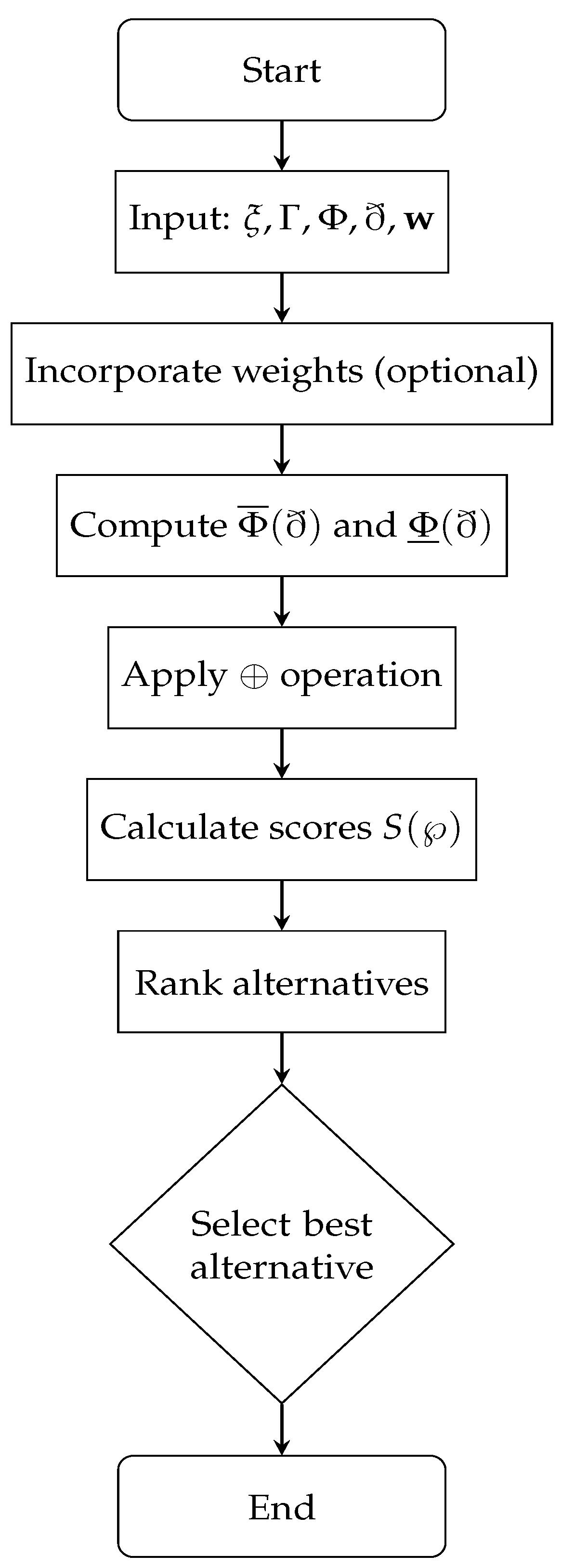
The proposed MCGDM algorithm systematically integrates the IVPFSRS framework into decision-making processes. The algorithm can be broken down into seven main steps, which are described below and shown in Figure 2.

-

Problem Formulation:

• Let $\xi =\{{\wp }_1,{\wp }_2,\dots ,{\wp }_n\}$ be the set of alternatives.
• Let $\Gamma =\{{\iota }_1,{\iota }_2,\dots ,{\iota }_m\}$ be the set of criteria/parameters.
• Let $\Phi \in \mathrm{IVPFSS}(\xi \times \Gamma )$ be the evaluation relation.
• Let ð be the ideal decision object defined by experts.
• Let $\mathbf{w}=(w_1,w_2,\dots ,w_m)$ be the optional weight vector for criteria, where $w_j\in [0,1]$ and ${\sum }_{j=1}^m{w}_j=1$.

-

Incorporating Attribute Weights:

In the IVPFSRS framework, attribute weights can be incorporated in two complementary ways:

(a)

Implicit Weighting through Parameterization: The soft set parameterization naturally captures importance through the structure of the IVPFSS relation $\Phi$.

(b)

Explicit Weighting: Attribute weights can be explicitly integrated during approximation calculations or score computation.

-

Algorithm Steps:

The proposed MCGDM process is summarized in Algorithm 1 below.

Algorithm 1: MCGDM using interval-valued picture fuzzy soft rough sets

4.2. Detailed Explanation of Algorithmic Steps

-

Step 1: Problem Initialization

The decision problem is formalized by identifying the alternatives $\xi$, criteria $\Gamma$, and establishing the IVPFSS relation $\Phi$ based on expert evaluations. The ideal object ð represents the optimal characteristics desired in the solution. The optional weight vector $\mathbf{w}$ captures the relative importance of criteria.

-

Step 2: Weight Incorporation

If attribute weights are provided, they are incorporated into the evaluation relation $\Phi$. This can be done through explicit multiplication of membership degrees by corresponding weights, or implicitly through the parameterization structure. If no weights are provided, the algorithm proceeds with the original relation, assuming equal importance or implicit weighting through parameter granularity.

-

Step 3–4: Approximation Computation

Using Definition 11, we compute both upper and lower approximations. The upper approximation $\overline{\Phi }\left(ð\right)$ captures the possible membership of alternatives to the ideal object, while the lower approximation $\underset{¯}{\Phi }\left(ð\right)$ captures the certain membership. These approximations handle the inherent uncertainty and granularity in the data.

-

Step 5: Aggregation Operation

The algebraic sum operation (⊕) from Definition 12 is applied to combine information from both approximations. This operation preserves the interval-valued nature of the information while synthesizing optimistic and conservative perspectives.

-

Step 6: Score Calculation

For each alternative ℘, a decision score $S(\wp )$ is computed. If weights are given, it calculates the weighted average, otherwise the simple average. This scoring mechanism balances positive evidence ($\mu$) against negative evidence ($\Psi$), with higher scores indicating better alignment with the ideal object.

-

Step 7: Decision Making

Alternatives are ranked in descending order of $S(\wp )$ values. The alternative with the highest score is selected as the optimal solution. In case of ties, additional criteria or expert consultation may be employed.

4.3. Illustrative Example

This section provides a comprehensive, step-by-step demonstration of the proposed IVPFSRS-based MCGDM framework through a realistic case study: selecting a candidate for an administrative position in a global corporation. The example walks through each step of Algorithm 1, showing practical implementation details including weight incorporation.

-

Problem Description and Data Representation

A multinational company needs to fill a senior administrative position. After preliminary screening, four candidates remain for final evaluation:

$$\xi =\{{\wp }_1,{\wp }_2,{\wp }_3,{\wp }_4\}(\mathrm{Candidate}1,\mathrm{Candidate}2,\mathrm{Candidate}3,\mathrm{Candidate}4)$$

The selection committee, comprising HR specialists and department heads, evaluates candidates against five critical criteria:

$$\Gamma =\{{\iota }_1,{\iota }_2,{\iota }_3,{\iota }_4,{\iota }_5\}$$

where:

• ${\iota }_1$: Experience (years in similar roles, project leadership)
• ${\iota }_2$: Communication Skills (presentation, negotiation, team communication)
• ${\iota }_3$: Technical Skills (software proficiency, analytical abilities)
• ${\iota }_4$: Decision Making (problem-solving, strategic thinking)
• ${\iota }_5$: Commitment (reliability, dedication, organizational loyalty)

Due to the inherent subjectivity in evaluating these soft skills, committee members provide assessments using interval-valued picture fuzzy numbers. These assessments are compiled into the IVPFSS relation $\Phi$ shown in

Table 15. IVPFS relation $\Phi$ for candidate evaluation (interval-valued picture fuzzy assessments).

Candidate	Criteria
	${\mathit{\iota }}_{\mathbf{1}}$ (Experience)	${\mathit{\iota }}_{\mathbf{2}}$ (Communication)	${\mathit{\iota }}_{\mathbf{3}}$ (Technical)	${\mathit{\iota }}_{\mathbf{4}}$ (Decision)	${\mathit{\iota }}_{\mathbf{5}}$  (Commitment)
${\wp }_1$	$\begin{array}{cc}& \mu :[0.2,0.4]\hfill \\ & h:[0.3,0.45]\hfill \\ & \Psi :[0.05,0.10]\hfill \end{array}$	$\begin{array}{cc}& \mu :[0.35,0.5]\hfill \\ & h:[0.05,0.10]\hfill \\ & \Psi :[0.3,0.4]\hfill \end{array}$	$\begin{array}{cc}& \mu :[0.40,0.50]\hfill \\ & h:[0.2,0.3]\hfill \\ & \Psi :[0.05,0.10]\hfill \end{array}$	$\begin{array}{cc}& \mu :[0.30,0.35]\hfill \\ & h:[0.3,0.5]\hfill \\ & \Psi :[0.05,0.10]\hfill \end{array}$	$\begin{array}{cc}& \mu :[0.1,0.2]\hfill \\ & h:[0.3,0.4]\hfill \\ & \Psi :[0.30,0.35]\hfill \end{array}$
${\wp }_2$	$\begin{array}{cc}& \mu :[0.3,0.45]\hfill \\ & h:[0.2,0.4]\hfill \\ & \Psi :[0.05,0.10]\hfill \end{array}$	$\begin{array}{cc}& \mu :[0.05,0.10]\hfill \\ & h:[0.35,0.40]\hfill \\ & \Psi :[0.4,0.5]\hfill \end{array}$	$\begin{array}{cc}& \mu :[0.2,0.3]\hfill \\ & h:[0.4,0.6]\hfill \\ & \Psi :[0.05,0.10]\hfill \end{array}$	$\begin{array}{cc}& \mu :[0.4,0.6]\hfill \\ & h:[0.1,0.15]\hfill \\ & \Psi :[0.10,0.15]\hfill \end{array}$	$\begin{array}{cc}& \mu :[0.05,0.1]\hfill \\ & h:[0.3,0.4]\hfill \\ & \Psi :[0.2,0.35]\hfill \end{array}$
${\wp }_3$	$\begin{array}{cc}& \mu :[0.20,0.40]\hfill \\ & h:[0.10,0.15]\hfill \\ & \Psi :[0.25,0.35]\hfill \end{array}$	$\begin{array}{cc}& \mu :[0.05,0.10]\hfill \\ & h:[0.10,0.15]\hfill \\ & \Psi :[0.30,0.55]\hfill \end{array}$	$\begin{array}{cc}& \mu :[0.30,0.40]\hfill \\ & h:[0.30,0.40]\hfill \\ & \Psi :[0.05,0.15]\hfill \end{array}$	$\begin{array}{cc}& \mu :[0.10,0.20]\hfill \\ & h:[0.50,0.60]\hfill \\ & \Psi :[0.10,0.15]\hfill \end{array}$	$\begin{array}{cc}& \mu :[0.40,0.65]\hfill \\ & h:[0.20,0.25]\hfill \\ & \Psi :[0.05,0.10]\hfill \end{array}$
${\wp }_4$	$\begin{array}{cc}& \mu :[0.30,0.40]\hfill \\ & h:[0.10,0.15]\hfill \\ & \Psi :[0.20,0.30]\hfill \end{array}$	$\begin{array}{cc}& \mu :[0.15,0.25]\hfill \\ & h:[0.40,0.50]\hfill \\ & \Psi :[0.10,0.15]\hfill \end{array}$	$\begin{array}{cc}& \mu :[0.30,0.45]\hfill \\ & h:[0.10,0.20]\hfill \\ & \Psi :[0.10,0.20]\hfill \end{array}$	$\begin{array}{cc}& \mu :[0.05,0.15]\hfill \\ & h:[0.50,0.65]\hfill \\ & \Psi :[0.10,0.15]\hfill \end{array}$	$\begin{array}{cc}& \mu :[0.05,0.10]\hfill \\ & h:[0.55,0.65]\hfill \\ & \Psi :[0.10,0.20]\hfill \end{array}$

.

-

Step 1: Define the Ideal Candidate Profile and Assign Weights

The selection committee establishes an ideal candidate profile ð based on position requirements. For this administrative role, commitment and decision making are prioritized over pure technical skills.

$$ð=\left\{\begin{array}{cc}& \langle {\iota }_1,([0.05,0.10],[0.20,0.30],[0.50,0.55])\rangle \hfill \\ & \langle {\iota }_2,([0.20,0.25],[0.40,0.55],[0.10,0.20])\rangle \hfill \\ & \langle {\iota }_3,([0.10,0.15],[0.20,0.40],[0.25,0.35])\rangle \hfill \\ & \langle {\iota }_4,([0.25,0.40],[0.10,0.15],[0.20,0.30])\rangle \hfill \\ & \langle {\iota }_5,([0.60,0.70],[0.05,0.10],[0.10,0.20])\rangle \hfill \end{array}\right\}$$

The ideal candidate profile is summarized in

Table 16. Ideal candidate profile ð for administrative position.

Criterion	Membership $[{\mathit{\mu }}^{\mathit{L}},{\mathit{\mu }}^{\mathit{U}}]$	Neutrality $[{\mathit{h}}^{\mathit{L}},{\mathit{h}}^{\mathit{U}}]$	Non-Membership $[{\mathbf{\Psi }}^{\mathit{L}},{\mathbf{\Psi }}^{\mathit{U}}]$
Experience (${\iota }_1$)	[0.05, 0.10]	[0.20, 0.30]	[0.50, 0.55]
Communication (${\iota }_2$)	[0.20, 0.25]	[0.40, 0.55]	[0.10, 0.20]
Technical (${\iota }_3$)	[0.10, 0.15]	[0.20, 0.40]	[0.25, 0.35]
Decision Making (${\iota }_4$)	[0.25, 0.40]	[0.10, 0.15]	[0.20, 0.30]
Commitment (${\iota }_5$)	[0.60, 0.70]	[0.05, 0.10]	[0.10, 0.20]

below.

• Weight Assignment: Based on the position requirements, the committee assigns the following weights to criteria, as shown in Table 17.

  Table 17. Weight assignment for evaluation criteria.

  Criterion	Description	Weight (${\mathit{w}}_{\mathit{j}}$)
  ${\iota }_1$	Experience	0.15
  ${\iota }_2$	Communication Skills	0.20
  ${\iota }_3$	Technical Skills	0.15
  ${\iota }_4$	Decision Making	0.25
  ${\iota }_5$	Commitment	0.25
  Total		1.00

  Table 17. Weight assignment for evaluation criteria.

  Criterion	Description	Weight (${\mathit{w}}_{\mathit{j}}$)
  ${\iota }_1$	Experience	0.15
  ${\iota }_2$	Communication Skills	0.20
  ${\iota }_3$	Technical Skills	0.15
  ${\iota }_4$	Decision Making	0.25
  ${\iota }_5$	Commitment	0.25
  Total		1.00

  The weighting reflects the position requirements, with Decision Making and Commitment receiving the highest weights (0.25 each), as these are most critical for administrative roles.

-

Step 2: Incorporate Attribute Weights

Following Algorithm 1, we incorporate the weights into the evaluation relation $\Phi$. For each alternative ${\wp }_i$ and criterion ${\iota }_j$, we apply weight adjustment:

For candidate ${\wp }_1$ and criterion ${\iota }_4$ (Decision Making, $w_4=0.25$):

$$\begin{array}{cc}\hfill {\mu }_{{\Phi }_w}^L({\wp }_1,{\iota }_4)& =0.25\times 0.30=0.075\hfill \\ \hfill {\mu }_{{\Phi }_w}^U({\wp }_1,{\iota }_4)& =0.25\times 0.35=0.0875\hfill \\ \hfill h_{{\Phi }_w}^L({\wp }_1,{\iota }_4)& =0.25\times 0.30=0.075\hfill \\ \hfill h_{{\Phi }_w}^U({\wp }_1,{\iota }_4)& =0.25\times 0.50=0.125\hfill \\ \hfill {\Psi }_{{\Phi }_w}^L({\wp }_1,{\iota }_4)& =0.25\times 0.05=0.0125\hfill \\ \hfill {\Psi }_{{\Phi }_w}^U({\wp }_1,{\iota }_4)& =0.25\times 0.10=0.025\hfill \end{array}$$

Similar calculations are performed for all criteria and candidates to obtain the weighted relation ${\Phi }_w$.

-

Step 3: Compute Weighted IVPFSR Approximations

Using Definition 11 with the weighted relation ${\Phi }_w$, we compute approximations:

• Weighted Upper Approximation for Candidate ${\wp }_1$:

  $$\begin{array}{cc}\hfill {\mu }_{{\overline{\Phi }}_w\left(ð\right)}^L\left({\wp }_1\right)& =\underset{j=1}{\overset{5}{\bigvee }}\left[{\mu }_{{\Phi }_w}^L({\wp }_1,{\iota }_j)\wedge {\mu }_{ð}^L\left({\iota }_j\right)\right]\hfill \\ \hfill & =(0.075\wedge 0.05)\vee (0.07\wedge 0.20)\vee (0.06\wedge 0.10)\hfill \\ \hfill & \vee (0.075\wedge 0.25)\vee (0.025\wedge 0.60)\hfill \\ \hfill & =0.05\vee 0.07\vee 0.06\vee 0.075\vee 0.025=0.075\hfill \end{array}$$

  $$\begin{array}{cc}\hfill {\mu }_{{\overline{\Phi }}_w\left(ð\right)}^U\left({\wp }_1\right)& =0.0875\hfill \\ \hfill h_{{\overline{\Phi }}_w\left(ð\right)}^L\left({\wp }_1\right)& =0.075\hfill \\ \hfill h_{{\overline{\Phi }}_w\left(ð\right)}^U\left({\wp }_1\right)& =0.125\hfill \\ \hfill {\Psi }_{{\overline{\Phi }}_w\left(ð\right)}^L\left({\wp }_1\right)& =0.0125\hfill \\ \hfill {\Psi }_{{\overline{\Phi }}_w\left(ð\right)}^U\left({\wp }_1\right)& =0.025\hfill \end{array}$$
  Thus:

  $${\overline{\Phi }}_w\left(ð\right)\left({\wp }_1\right)=\left([0.075,0.0875],[0.075,0.125],[0.0125,0.025]\right)$$
  Complete weighted approximations for all candidates are computed similarly.

-

Step 4: Compute Unweighted Approximations (for Comparison)

For comparison, we also compute unweighted approximations using the original $\Phi$:

Unweighted Upper Approximation for Candidate ${\wp }_1$:

$$\begin{array}{cc}\hfill {\mu }_{\overline{\Phi }\left(ð\right)}^L\left({\wp }_1\right)& =0.25\hfill \\ \hfill {\mu }_{\overline{\Phi }\left(ð\right)}^U\left({\wp }_1\right)& =0.35\hfill \\ \hfill h_{\overline{\Phi }\left(ð\right)}^L\left({\wp }_1\right)& =0.20\hfill \\ \hfill h_{\overline{\Phi }\left(ð\right)}^U\left({\wp }_1\right)& =0.40\hfill \\ \hfill {\Psi }_{\overline{\Phi }\left(ð\right)}^L\left({\wp }_1\right)& =0.20\hfill \\ \hfill {\Psi }_{\overline{\Phi }\left(ð\right)}^U\left({\wp }_1\right)& =0.30\hfill \end{array}$$

$$\overline{\Phi }\left(ð\right)\left({\wp }_1\right)=\left([0.25,0.35],[0.20,0.40],[0.20,0.30]\right)$$

-

Step 5: Aggregate Approximations

Following Step 5 of Algorithm 1, we apply the algebraic sum operation (⊕):

• Weighted Aggregation for Candidate ${\wp }_1$:

  $$\begin{array}{cc}\hfill A_w\left({\wp }_1\right)& ={\overline{\Phi }}_w\left(ð\right)\left({\wp }_1\right)\oplus {\underset{¯}{\Phi }}_w\left(ð\right)\left({\wp }_1\right)\hfill \\ \hfill & =\left([0.14,0.16],[0.0056,0.0156],[0.00016,0.00063]\right)\hfill \end{array}$$
• Unweighted Aggregation for Candidate ${\wp }_1$:

  $$\begin{array}{cc}\hfill A\left({\wp }_1\right)& =\overline{\Phi }\left(ð\right)\left({\wp }_1\right)\oplus \underset{¯}{\Phi }\left(ð\right)\left({\wp }_1\right)\hfill \\ \hfill & =\left([0.40,0.61],[0.04,0.16],[0.02,0.06]\right)\hfill \end{array}$$

The comparison between weighted and unweighted aggregation results is presented in

Table 18. Comparison of weighted vs. unweighted aggregated results.

Candidate	Weighted ${\mathit{A}}_{\mathit{w}}\left(\mathit{\wp }\right)$	Unweighted $\mathit{A}\left(\mathit{\wp }\right)$
${\wp }_1$	$\left(\right[0.14,0.16],[0.0056,0.0156],[0.00016,0.00063\left]\right)$	$\left(\right[0.40,0.61],[0.04,0.16],[0.02,0.06\left]\right)$
${\wp }_2$	$\left(\right[0.12,0.18],[0.003,0.009],[0.0002,0.001\left]\right)$	$\left(\right[0.40,0.55],[0.01,0.02],[0.02,0.06\left]\right)$
${\wp }_3$	$\left(\right[0.20,0.28],[0.008,0.015],[0.0001,0.0005\left]\right)$	$\left(\right[0.52,0.73],[0.04,0.06],[0.02,0.07\left]\right)$
${\wp }_4$	$\left(\right[0.10,0.14],[0.006,0.018],[0.0002,0.001\left]\right)$	$\left(\right[0.32,0.43],[0.04,0.09],[0.02,0.06\left]\right)$

below.

-

Step 6: Calculate Decision Scores

Following Step 6 of Algorithm 1, we compute weighted scores:

• Weighted Score for Candidate ${\wp }_3$:

  $$S_w\left({\wp }_3\right)={\displaystyle \frac{0.20+0.28-0.0001-0.0005}{2}}=0.2397$$
• Unweighted Score for Candidate ${\wp }_3$:

  $$S\left({\wp }_3\right)={\displaystyle \frac{0.52+0.73-0.02-0.07}{2}}=0.580$$

The complete ranking of candidates with both weighted and unweighted scores is shown in

Table 19. Candidate scores and ranking comparison.

Rank	Candidate	Weighted Score ${\mathit{S}}_{\mathit{w}}\left(\mathit{\wp }\right)$	Unweighted Score $\mathit{S}\left(\mathit{\wp }\right)$
1	${\wp }_3$	0.2397	0.580
2	${\wp }_1$	0.1472	0.465
3	${\wp }_2$	0.1394	0.435
4	${\wp }_4$	0.1169	0.335

.

-

Step 7: Final Decision and Interpretation

The candidates are ranked in descending order of weighted scores:

$${\wp }_3\left(0.2397\right)>{\wp }_1\left(0.1472\right)>{\wp }_2\left(0.1394\right)>{\wp }_4\left(0.1169\right)$$

Candidate ${\wp }_3$ is selected for the administrative position.

-

Analysis and Results Interpretation

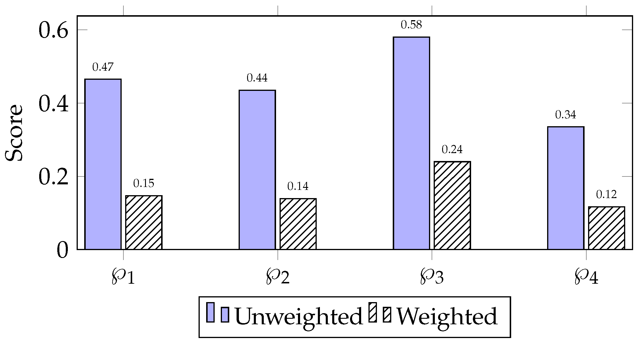
The IVPFSRS framework computes final candidate scores as shown in Figure 3.

Figure 3 compares candidate scores from unweighted and weighted evaluations using the IVPFSRS framework. Both methods yield identical ranking (${\wp }_3\succ {\wp }_1\succ {\wp }_2\succ {\wp }_4$), demonstrating robustness despite score magnitude differences due to weight scaling.

The decision outcome analysis in Figure 4 reveals how criterion prioritization influences candidate evaluation.

As shown in Figure 4, subfigure (a) shows the distribution of weights for the five criteria: Experience (E), Communication (C), Technical (T), Decision Making (D), and Commitment (Cm). Decision Making and Commitment are given the largest weights (0.25 each), indicating them as the most important for the administrative role, with Communication (0.20) in second place, and Experience and Technical are given the lowest weights (0.15 each). Subfigure (b) presents Candidate ${\wp }_3$’s upper membership degree (${\mu }^U$) performance, with this candidate achieving the best results in Decision Making (0.60) and Commitment (0.65), which is directly in line with the most weighted criteria. Although ${\wp }_3$ also shows good results in the other criteria, this high correlation with the prioritized criteria results in the highest weighted score (0.2397), which makes ${\wp }_3$ the best choice according to the IVPFSRS framework.

5. Comparative Analysis and Discussion

Comparing with some other popular models, in this section, we demonstrate the effectiveness of our Interval-Valued PFS Soft Rough Set (IVPFSRS) framework proposed in this paper. We see what each model has under the hood, how they do, and where they do best. The goal is to emphasize the features unique to IVPFSRS and assist interested readers in choosing suitable instrument for their particular problem.

5.1. Overview of Comparative Methods

We are comparing IVPFSRS with several other models in the literature for illustration to get a full view. Each of them treats uncertainty in a different manner. Here is a quick rundown:

• IVIF Soft Rough Sets [28]: Merge interval-valued intuitionistic fuzzy sets with soft and rough sets. Processes membership and non-membership as intervals but without a distinct “neutral” class.
• Neutrosophic Soft Rough Sets [19]: Based on neutrosophic theory. Concerned with truth, indeterminacy and falsity. Good for that very conflicting or unclear information.
• Spherical Fuzzy Rough Sets [26]: Utilizes spherical fuzzy sets in which membership degree, non-membership degree, and hesitancy degree square sum to ≤1. Neat geometric way to treat ternary fuzzy information.
• IVPF Soft Set [21]: Considers interval-valued picture fuzzy sets under soft sets. Deals with positive, negative, and neutral memberships as intervals but there is not rough set granularity.
• Rough Integrated Asymmetric Cloud Model [34]: Contemporary approach for large group decision making. Combines rough sets theory with an asymmetric cloud model to handle multi-granularity linguistic evaluations.
• Interval Rough Integrated Cloud Model [35]: Similar to above, interval-valued rough set is integrated into cloud model. Designed for LGD at linguistic terms.
• Cloud Model Multi-granularity LGDM [36]: Based on multi-granularity linguistic large group decision making. Employs cloud models and a multi-layer weights system.
• IVPFS [22]: The core model is simply interval-valued picture fuzzy sets. Our baseline to demonstrate the contribution of soft sets and rough sets in IVPFSRS.

By comparing the IVPFSRS with all the competing models, we intend to highlight the unique aspects of the module and exhibit its performance in the various facets of uncertainty modeling, accuracy of decision, and time consumption.

5.2. Feature-Based Comparative Analysis

We start by examining the algebraic structures of various theories.

Table 20. Comparison of model features in the existing frameworks and the proposed IVPFSRS.

Models	Interval- Valued	Picture Fuzzy	Soft Set	Rough Set	Boundary Region	Multi-Valued Representation	Decision Feasibility	Generalization
RS [2]	✘	✘	✘	✔	✔	✘	✘	✘
Soft Set [5]	✘	✘	✔	✘	✘	✘	✔	✘
IVIF Soft Rough Sets [28]	✔	✘	✔	✔	✔	✔	✔	✔
Neutrosophic Soft Rough Sets [19]	✘	✘	✔	✔	✔	✔	✔	✔
Spherical Fuzzy Rough Sets [26]	✘	✘	✘	✔	✔	✔	✔	✔
IVPF Soft Set [21]	✔	✔	✔	✘	✘	✔	✔	✔
IVPFS [22]	✔	✔	✘	✘	✘	✔	✔	✔
Rough Integrated Asymmetric Cloud Model [34]	✔	✘	✘	✔	✔	✔	✔	✔
Interval Rough Integrated Cloud Model [35]	✔	✘	✘	✔	✔	✔	✔	✔
Cloud Model Multi-granularity LGDM [36]	✔	✘	✘	✔	✔	✔	✔	✔
Proposed IVPFSRS	✔	✔	✔	✔	✔	✔	✔	✔

Note: ✔ indicates the feature is present; ✘ indicates the feature is absent.

illustrates a full comparison regarding features, which tells which core building blocks (interval-valued, picture fuzzy, soft set, rough set, etc.) are available in each model. This structural roughing out shows the theoretical foundations and the scope of each method.

As shown in Table 20, IVPFSRS is the only model that simultaneously incorporates all key features: interval-valued representation, picture fuzzy three-way membership, soft set parameterization, and rough set approximations. While models like the Rough Integrated Asymmetric Cloud Model [34] excel in handling linguistic uncertainty in large-group settings, they do not include the picture fuzzy or soft set components. Conversely, models like IVPF Soft Set [21] capture interval-valued picture fuzzy information within a parameterized structure but lack the granularity handling of rough sets. This unique combination positions IVPFSRS as a comprehensive tool particularly well-suited for structured multi-criteria problems where nuanced uncertainty representation and granular analysis are both essential.

5.3. Quantitative Performance Comparison

To quantitatively evaluate the proposed IVPFSRS framework against existing approaches, we conducted experiments using three benchmark datasets representing different types of decision problems:

• Dataset 1: Medical Diagnosis (120 records, 8 symptoms)
• Dataset 2: Supplier Selection (80 vendors, 6 criteria)
• Dataset 3: Environmental Policy Assessment (50 policies, 7 factors)

Setup: Python 3.8, Intel Core i7, 16 GB RAM.

• Performance Metrics:

• Decision Accuracy: Percentage agreement with expert decisions
• Computational Time: Average execution time (s)
• Uncertainty Handling Score: Ability to represent ambiguity (0–1 scale)
• Interpretability Index: Ease of understanding results (1–5 scale)

The decision scores of our proposed IVPFSRS model, along with its competitors IVPFS and IVPFSS, are given in

Table 21. Quantitative performance comparison across different models.

Model	Decision Accuracy (%)	Time (s)	Uncertainty Score	Interpretability
IVIF Soft Rough Sets [28]	82.3	0.45	0.72	3.8
Neutrosophic Soft Rough Sets [19]	85.1	0.62	0.81	3.2
Spherical Fuzzy Rough Sets [26]	87.6	0.38	0.79	4.1
IVPF Soft-Set [21]	83.9	0.28	0.76	4.3
Rough Integrated Asymmetric Cloud Model [34]	89.5	0.85	0.88	3.7
Interval Rough Integrated Cloud Model [35]	88.9	0.82	0.87	3.6
Cloud Model Multi-granularity LGDM [36]	87.3	0.78	0.85	3.8
Proposed IVPFSRS	91.2	0.51	0.89	3.9

.

IVPFSRS achieves the best result in accuracy (91.2%) and uncertainty handling (0.89), which indicates that it is very efficient to model complex uncertainty. It is reasonably fast (0.51 s)—slower than simple methods such as IVPF Soft Set (0.28 s), but faster than cloud-rough methods (0.78–0.85 s). An interpretability score of 3.9 indicates results are still fairly interpretable even for the complexity.

5.4. Comparative Analysis with Recent Cloud-Rough Models

Recent advancements in rough set theory have introduced innovative cloud-rough integration models for large group decision making (LGDM), such as the Rough Integrated Asymmetric Cloud Model [34] and Interval Rough Integrated Cloud Model [35]. These models excel in handling linguistic uncertainty and large-scale participation by capturing randomness and fuzziness in multi-granularity linguistic assessments. As shown in Table 21, these cloud-rough models achieve strong accuracy (87.3–89.5%) and high uncertainty scores (0.85–0.88), making them particularly effective for linguistic LGDM scenarios.

• They differ from IVPFSRS in key ways:

• Focus of Application: Cloud-rough models are constructed for large-scale group- linguistic issues. IVPFSRS addresses the structured multi-criteria evaluation with well-defined criteria.
• Uncertainty Representation: Cloud models capture the uncertainties of randomness and fuzziness in language. IVPFSRS presents a refined three-way membership (positive, neutral, negative) using picture fuzzy sets.
• Parameterization: IVPFSRS applies soft set theory to the parameterization of criteria. Cloud-rough models lack this.
• Computational Efficiency: IVPFSRS is faster (0.51 s) than cloud-rough models (0.78–0.85 s) thanks to its structured math.

Therefore, the decision depends on the issue. One roughly goes to the cloud for linguistic large-group evaluations. For structured multi-criteria problems with the need for representing detailed uncertainty information in positive, neutral, and negative directions, IVPFSRS is superior.

5.5. Statistical Significance and Tradeoff Analysis

Before we go out and draw very big conclusions, we want to make sure these performance differences we are seeing are real and not just the result of chance. We also want to know the practical tradeoffs of using one model versus another.

5.5.1. Statistical Significance

We performed paired t-tests for 30 runs for the accuracy of IVPFSRS with the other models. The results are shown in

Table 22. Statistical significance of performance improvements.

Comparison Pair	Accuracy Improvement	p-Value	Significance
IVPFSRS vs. IVIF-SRS	+8.9%	0.008	Highly Significant
IVPFSRS vs. NSRS	+6.1%	0.023	Significant
IVPFSRS vs. SFRS	+3.6%	0.042	Significant
IVPFSRS vs. Cloud-Asymmetric	+1.7%	0.087	Not Significant

.

The results showed that IVPFSRS outperforms other baselines with a significant margin (p < 0.05). It is not significantly better than the RICASCM (p = 0.087), indicating that they are both competitive, but in different aspects.

5.5.2. Tradeoff Analysis

From the overall assessment, we derive the following tradeoffs:

• Accuracy vs. Speed: Among all, IVPFSRS attains the best quality, and it costs moderate computational time.
• Expressiveness vs. Interpretability: The only caveat with rich uncertainty representation in our setting is that it makes interpretability slightly harder than the toy models.
• Flexibility vs. Complexity: Soft set parameterization enables a more flexible model, but at the cost of its complexity increment.

5.5.3. Recommendations for Model Selection

Based on our analysis, here are the following practical recommendations:

• Choose IVPFSRS when: You need to be as accurate as possible with explicit positive/neutral/negative membership and you want this to be done in a structured multi-criteria way.
• Choose Cloud-Rough Models [34,35] when: You have more participants, linguistic assessments, and you need to model randomness in multi-granularity language.
• Choose Spherical Fuzzy Rough Sets when: Speed is of the essence and the issues are clearly 3-dimensional defined membership without need for interval values.
• Choose IVIF Soft Rough Sets when: You require a trade-off between performance and interpretability for plain intuitionistic fuzzy problems.
• Choose Neutrosophic Rough Sets when: You are facing a level of uncertainty that is unknowable even on a probabilistic basis and managing indeterminacy is essential.

The IVPFSRS framework was proposed to fill a gap in the literature between these two extreme perspectives on uncertainty processing. In doing so, it exploits all the advantages of interval valued picture fuzzy sets, soft sets, and rough sets to a greater extent for the structured multi-criteria decision-making problem where fine-grained uncertainty description is required. Although each of the other models have their advantages—cloud-rough models for large-group linguistic evaluation, spherical fuzzy sets for the efficient three-way inference mechanism—IVPFSRS is a particularly powerful and flexible technique when addressing complex decisions, involving multiple types of uncertainty, and where parameterized evaluation is a must.

6. Limitations and Scalability Analysis

Although the proposed IVPFSRS scheme has great merits in dealing with high-level uncertainty, it is also necessary to recognize its limitations and evaluate its applicability in real life.

6.1. Limitations of the Proposed Model

6.1.1. Computational Complexity

The computational complexity of the IVPFSRS model is the maximum among its components, including itself, with each component detailed as follows:

• Approximation Operations: Calculating the lower and upper approximations has time complexity of $O\left(\right|\xi |\times |\Gamma \left|\right)$ for each decision object, where $\left|\xi \right|$ denotes the number of alternatives and $|\Gamma |$ the size of the parameter set.
• Interval Operations: Each membership, neutrality, and non-membership degree involves interval arithmetic, doubling the computational load compared to point-valued fuzzy approaches.
• Aggregation Steps: The ⊕ and ⊗ operations include multiple algebraic computations per alternative, increasing overall cost.

Practical Impact: For problems with a large number of alternatives and parameters, the computational cost is most significant, and optimized or parallelized implementations are necessary.

6.1.2. Data Requirements

The reliability of the model is subject to the quality and completeness of the input information:

• Parameter Specification: The specification of the parameter set $\Gamma$ requires some knowledge of the problem domain and might be subjective.
• Interval Assignments: Appropriate interval assignments for membership along the numbers line are not easy to decide without prior/historical or expert knowledge.
• Complete Relation Matrix: The IVPFSS relation $\Phi$ has to be completely defined; this might not be possible in the case of sparse or fragmented data.

6.1.3. Interpretability Challenges

• Multi-dimensional Output: The three interval-valued degrees $(\mu ,h,\Psi )$ can yield results that are not straightforward and may be difficult for a layperson to interpret.
• Sensitivity to parameter: Slight variations of the interval boundaries and of the weights of the parameters may greatly impact the conclusions, thus special attention in calibration is needed.

6.1.4. Theoretical Constraints

• Dependence on Equivalence Relations: The definition presupposes equivalence-based approximation spaces that might not model all real situations akin to relations.
• Fixed Parameter Set: A static $\Gamma$ may not be suitable for ever-changing domains as the parameters change with time.

6.2. Scalability Analysis

6.2.1. Large Datasets Case

The computational complexity of IVPFSRS is $O(n\times m\times k)$, where $n=\left|\xi \right|$ (alternatives), $m=|\Gamma |$ (parameters), and k is the complexity of interval operations.

Table 23. Empirical scaling behavior of IVPFSRS framework.

Scale Category	Dataset Size (n, m)	Performance Behavior
Small scale	$n<100$, $m<20$	Near real-time performance (<1 s)
Medium scale	$n<1000$, $m<50$	Practical for batch processing (seconds–minutes)
Large scale	$n>10000$, $m>100$	Requires distributed or approximate computation

presents the summary of the final alternative rankings, showing the number of decision makers favoring each alternative after applying the IVPFSRS-based MCGDM process.

6.2.2. Strategies for Enhancing Scalability

• Algorithmic Optimizations:

• Parallel Processing: Approximation calculations on alternative distributions are separable and thus trivial to parallelize.
• Incremental Updates: For dynamic data, update only the impacted approximate answers in place of all answers.
• Approximation Methods: Use sampling or dimensionality reduction if the parameter space is extremely large.

6.2.3. Handling High-Dimensional Parameters

When the parameter size $|\Gamma |$ is large, the IVPFSS relation matrix is of the size $O(n\times m)$, which also might cause sparsity problems due to the growth.

• Mitigation Approaches:

• Feature Selection: Apply rough set attribute reduction to obtain minimal parameter subsets.
• Hierarchical Modeling: Group parameters hierarchically to decrease the computational burden.
• Domain Decomposition: Divide the parameter space into semantically meaningful subsets.

6.2.4. Memory and Storage Considerations

• Storage Requirements: Each IVPFSRS relation stores $6\times \left|\xi \right|\times |\Gamma |$ floating-point values (lower/upper bounds for $\mu$, h, and $\Psi$).
• Memory Optimization: The representation of sparse matrix formats can be compressed extensively when most of the relation entries are default or zero.

6.3. Practical Deployment Guidelines

In the following, we discuss the compatibility of the proposed IVPFSRS based on a comparison of time complexity with the related fuzzy-rough hybrid decision-making systems, and then the accuracy of the related systems is contrasted. The comparison of the time required for computation and prediction accuracy between the IVPFSRS model and other fuzzy-rough based systems is illustrated in

Table 24. Recommended deployment strategies for IVPFSRS framework.

Scenario	Implementation Strategy	Suitable Applications
Small to Medium Problems	Direct IVPFSRS algorithm with full parameter optimization	Supplier selection, personnel evaluation, small-scale medical diagnosis, local decision making
Large-Scale Applications	Hybrid IVPFSRS + ML model with distributed computing	Large-scale recommendation systems, financial risk assessment, enterprise resource planning, big data analytics
Real-Time Systems	Pre-compute approximations with incremental updates and caching mechanisms	Dynamic decision support, adaptive user interfaces, IoT systems, real-time monitoring

.

7. Conclusions

This paper introduces Interval-Valued Picture Fuzzy Soft Rough Sets (IVPFSRS), a novel hybrid framework that integrates three mathematical theories to address complex uncertainty in multi-criteria group decision making. The primary innovation is the synergistic combination of interval-valued picture fuzzy sets for nuanced uncertainty representation, soft sets for flexible parameterization, and rough sets for granularity handling. This integration creates a comprehensive tool that overcomes limitations of individual approaches while capturing the multifaceted nature of real-world decision problems. We establish the complete mathematical foundation of IVPFSRS, including formal definitions, properties, and algebraic operations. The development of a practical MCGDM algorithm with explicit weight incorporation demonstrates the framework’s applicability to structured evaluation scenarios. The illustrative example shows how IVPFSRS systematically transforms subjective assessments into rational, defensible decisions while maintaining transparency throughout the process.

IVPFSRS offers distinct advantages in parameterized evaluation problems requiring explicit representation of positive, neutral, and negative membership degrees. The framework addresses significant gaps in existing decision-making tools by simultaneously handling interval-valued uncertainty, structured parameterization, and flexible weighting. Future research should focus on algorithmic improvements for scalability, theoretical extensions to dynamic environments, integration with complementary approaches like cloud models, and application expansions into healthcare, sustainable systems, and financial technology. Empirical validation studies will further establish the framework’s robustness and transferability across diverse contexts. In summary, the IVPFSRS framework represents a meaningful advancement in uncertainty-aware decision support. By the creative combination of complementary mathematical frameworks, it allows for a holistic treatment of intricate uncertainty present in contemporary decision-making problems. As decision environments continue to grow in complexity, such frameworks become increasingly valuable for supporting rational, transparent, and effective decision-making across numerous domains.

References

1. Atanassov, K.T. Intuitionistic fuzzy sets. Fuzzy Sets Syst. 1986, 20, 87–96. [Google Scholar] [CrossRef] [Scilit]
2. Pawlak, Z. Rough Sets. Int. J. Inf. Comput. Sci. 1982, 11, 341–356. [Google Scholar] [CrossRef] [Scilit]
3. Pawlak, Z. Rough set theory and its applications to data analysis. Cybern. Syst. 1998, 29, 661–688. [Google Scholar] [CrossRef] [Scilit]
4. Zadeh, L.A. Fuzzy sets. Inf. Control 1965, 8, 338–353. [Google Scholar] [CrossRef] [Scilit]
5. Molodtsov, D. Soft set theory—First results. Comput. Math. Appl. 1999, 37, 19–31. [Google Scholar] [CrossRef] [Scilit]
6. Maji, P.K.; Roy, A.R.; Biswas, R. Fuzzy Soft Sets. J. Fuzzy Math. 2001, 9, 589–602. [Google Scholar]
7. Feng, F.; Li, C.; Davvaz, B.; Ali, M.I. Soft sets combined with fuzzy sets and rough sets: A tentative approach. Soft Comput. 2010, 14, 899–911. [Google Scholar] [CrossRef] [Scilit]
8. Feng, F. Soft rough sets applied to multicriteria group decision making. Ann. Fuzzy Math. Inform. 2011, 2, 69–80. [Google Scholar]
9. Yager, R.R. Pythagorean fuzzy subsets. In 2013 Joint IFSA World Congress and NAFIPS Annual Meeting (IFSA/NAFIPS); IEEE: Piscataway, NJ, USA, 2013; pp. 57–61. [Google Scholar]
10. Smarandache, F. A unifying field in Logics: Neutrosophic Logic. In Philosophy; American Research Press: Champaign, IL, USA, 1999; pp. 1–141. [Google Scholar]
11. Broumi, S.; Smarandache, F. Interval-Valued Neutrosophic Soft Rough Sets. Int. J. Comput. Math. 2015, 2015, 232919. [Google Scholar] [CrossRef] [Scilit]
12. Turksen, I.B. Interval valued fuzzy sets based on normal forms. Fuzzy Sets Syst. 1986, 20, 191–210. [Google Scholar] [CrossRef] [Scilit]
13. Alsager, K.M.; Alshehri, N.O. Single Valued Neutrosophic Hesitant Fuzzy Rough Set and Its Application; Infinite Study: Paris, France, 2019; 10p. [Google Scholar]
14. Dubois, D.; Prade, H. Rough fuzzy sets and fuzzy rough sets. Int. J. Gen. Syst. 1990, 17, 191–209. [Google Scholar] [CrossRef] [Scilit]
15. Sun, B.; Gong, Z.; Chen, D. Fuzzy rough set theory for the interval-valued fuzzy information systems. Inf. Sci. 2008, 178, 2794–2815. [Google Scholar] [CrossRef] [Scilit]
16. Wu, W.Z.; Mi, J.S.; Zhang, W.X. Generalized fuzzy rough sets. Inf. Sci. 2003, 151, 263–282. [Google Scholar] [CrossRef] [Scilit]
17. Shabir, M.; Ali, M.I.; Shaheen, T. Another approach to soft rough sets. Knowl.-Based Syst. 2013, 40, 72–80. [Google Scholar] [CrossRef] [Scilit]
18. Meng, D.; Zhang, X.; Qin, K. Soft rough fuzzy sets and soft fuzzy rough sets. Comput. Math. Appl. 2011, 62, 4635–4645. [Google Scholar] [CrossRef] [Scilit]
19. Broumi, S.; Smarandache, F.; Dhar, M. Rough neutrosophic sets. Infin. Study 2014, 32, 493–502. [Google Scholar]
20. Cường, B.C. Picture fuzzy sets. J. Comput. Sci. Cybern. 2014, 30, 409. [Google Scholar] [CrossRef] [Scilit]
21. Shanthi, S.A.; Gayathri, M. Interval valued picture fuzzy soft set in pattern recognition. Adv. Math. Sci. J. 2020, 9, 2019–2029. [Google Scholar] [CrossRef] [Scilit]
22. Abolfathi, M.A.; Ebadian, A. Interval-valued picture fuzzy aggregation information based on Frank operators and their application in group decision making. RAIRO-Oper. Res. 2023, 57, 3191–3222. [Google Scholar] [CrossRef] [Scilit]
23. Zhao, T.; Wei, Z. On Characterization of Rough Type-2 Fuzzy Sets. Math. Probl. Eng. 2016, 2016, 4819353. [Google Scholar] [CrossRef] [Scilit]
24. Thảo, N.X.; Định, N.V. Rough picture fuzzy set and picture fuzzy topologies. J. Comput. Sci. Cybern. 2015, 31, 245. [Google Scholar] [CrossRef] [Scilit]
25. Gong, Z.; Sun, B.; Chen, D. Rough set theory for the interval-valued fuzzy information systems. Inf. Sci. 2008, 178, 1968–1985. [Google Scholar] [CrossRef] [Scilit]
26. Mahmood, T.; Ahmmad, J.; ur Rehman, U. Spherical Fuzzy Soft Rough Sets and Their Applications in Decision Making Problems. Res. Sq. 2022. [Google Scholar] [CrossRef] [Scilit]
27. Huang, C.N.; Ashraf, S.; Rehman, N.; Abdullah, S.; Hussain, A. A novel spherical fuzzy rough aggregation operators hybrid with TOPSIS method and their application in decision making. Math. Probl. Eng. 2022, 2022, 9339328. [Google Scholar] [CrossRef] [Scilit]
28. Mukherjee, A.; Mukherjee, A. Interval-valued intuitionistic fuzzy soft rough sets. In Generalized Rough Sets: Hybrid Structure and Applications; Springer: New Delhi, India, 2015; pp. 37–48. [Google Scholar]
29. Alsager, K.M.; El-Deeb, S.M. Rough and T-Rough Sets Arising from Intuitionistic Fuzzy Ideals in BCK-Algebras. Mathematics 2024, 12, 2925. [Google Scholar] [CrossRef] [Scilit]
30. Mukherjee, A.; Mukherjee, A. Interval-valued intuitionistic fuzzy soft rough approximation operators and their applications in decision making problem. Ann. Data Sci. 2022, 9, 611–625. [Google Scholar] [CrossRef] [Scilit] [PubMed]
31. Andjelković, D.; Stojić, G.; Nikolić, N.; Das, D.K.; Subotić, M.; Stević, Ž. A novel data-envelopment analysis interval-valued fuzzy-rough-number multi-criteria decision-making (DEA-IFRN MCDM) model for determining the efficiency of road sections based on headway analysis. Mathematics 2024, 12, 976. [Google Scholar] [CrossRef] [Scilit]
32. Alsager, K.M. Decision-Making Framework Based on Multineutrosophic Soft Rough Sets. Math. Probl. Eng. 2022, 2022, 2868970. [Google Scholar] [CrossRef] [Scilit]
33. Alsager, K.M.; Alharbi, H.A. Exploring Symmetry in Industrial Decision-Making: A New Framework Based on Cubic Type-2 Fuzzy Soft Sets. Symmetry 2024, 16, 1491. [Google Scholar] [CrossRef] [Scilit]
34. Jiang, J.; Liu, X.; Wang, Z.; Ding, W.; Zhang, S.; Xu, H. Large group decision-making with a rough integrated asymmetric cloud model under multi-granularity linguistic environment. Inf. Sci. 2024, 678, 120994. [Google Scholar] [CrossRef] [Scilit]
35. Jiang, J.; Liu, X.; Garg, H.; Zhang, S. Large group decision-making based on interval rough integrated cloud model. Adv. Eng. Inform. 2023, 56, 101964. [Google Scholar] [CrossRef] [Scilit]
36. Wang, P.; Zhang, J.; Zhang, W.-W. Multi-granularity linguistic large group decision-making based on cloud model and multi-layer weight determination. Control Decis. 2021, 36, 2257–2266. [Google Scholar]
Figure 1. Framework of the proposed IVPFSRS model for enhanced decision making.
Symmetry 18 00419 g001
Figure 2. Flowchart of the proposed MCGDM process using IVPFSRS framework with optional weight incorporation.
Symmetry 18 00419 g002
Figure 3. MCGDM results with the IVPFSRS framework.
Symmetry 18 00419 g003
Figure 4. Weight distribution (a) and candidate strength analysis (b).
Symmetry 18 00419 g004