Article

Analysis of Reaction-Diffusion Systems: Painlevé Properties and Conservation Laws of the Convective Fisher–Kolmogorov Equations


by
Ali Raza
1,2,*,
Alhussein Mohamed Alhussein Ahmed
3 and
Abdul Hamid Kara
4
1
Department of Mathematical Sciences, Stellenbosch University, Stellenbosch 7602, South Africa
2
Centre for Mathematics and Statistical Sciences, Lahore School of Economics, Lahore 53200, Pakistan
3
School of Computer Science and Applied Mathematics, University of the Witwatersrand, Johannesburg 2050, South Africa
4
School of Mathematics, University of the Witwatersrand, Johannesburg 2050, South Africa
*
Author to whom correspondence should be addressed.
Symmetry 2026, 18(2), 377; https://doi.org/10.3390/sym18020377
Submission received: 10 January 2026 / Revised: 12 February 2026 / Accepted: 16 February 2026 / Published: 18 February 2026
(This article belongs to the Special Issue Symmetry in Lie Groups and Lie Algebras)

Abstract

This article investigates the widespread occurrence of wave-like behavior in biological systems and reflects on the importance of reaction–diffusion frameworks to explain fast information transfer. Focusing on the classical Fisher–Kolmogorov equation, it demonstrates how the combination of nonlinear reaction dynamics and diffusion gives rise to stable traveling wavefronts that propagate at a constant speed while preserving their shape. We adopt a number of approaches (some novel) in dealing with the analyses, namely the symmetry method, soliton approach (algebraic) and Painlevé analysis, among others.

1. Introduction

Biological waves play a central role in developmental processes, appearing in forms such as chemical concentration patterns, mechanical deformations, and electrical signaling. These wave phenomena arise across a wide range of biological systems, including mechanical waves in fish eggs, chemical oscillations in the Belousov–Zhabotinskii reaction, insect dispersal dynamics and interacting population models. Representative examples include the spread of epidemics, directed movement of microorganisms toward nutrient sources, and chemotactic aggregation in slime molds. The regularity of such wave-like behavior throughout the biomedical sciences underscores the significance of studying traveling waves and developing appropriate mathematical models and analytical tools to understand them.
Rhythmic and wave-like patterns frequently emerge in the early stages of embryonic development, indicating their essential role in coordinating growth and differentiation. Chemical concentration waves also occur in other contexts, notably in the Belousov–Zhabotinsky reaction, which serves as a model system for self-organizing biochemical dynamics. Comparable reaction–diffusion mechanisms are active in living tissues, where they support pattern formation and enable coordinated signaling among cells.
Beyond the cellular scale, wave propagation plays a key role in ecological and population dynamics, producing invasion fronts and dispersal waves in interacting populations. The spread of infectious diseases, including rabies epidemics, can be effectively described using traveling wave models. Chemotaxis provides another prominent example: microorganisms migrate in response to chemical cues, as observed in Dictyostelium discoideum, where periodic chemical signaling directs coordinated cell movement during aggregation.
The study of biological waves has a rich interdisciplinary history [1], providing numerous examples linking oscillations and waves to biological rhythms. Earlier foundational work, such as [2], addressed wave behavior in mathematical models of molecular and cellular biology, and the more mathematically oriented studies of [3,4] explored the theoretical structure of reaction–diffusion systems. From another viewpoint, biological waves can be approached through the framework of catastrophe theory, examining how small changes can produce large-scale structural transitions in developing organisms.
Wave phenomena are central to communication and coordination in living systems, with multicellular organisms relying on continuous information transfer for complex organization, particularly in embryo genesis for tissue formation and morphology. Biochemical signaling waves are key mechanisms for this communication. However, pure diffusion alone cannot explain the observed propagation speeds in these systems, as diffusion coefficients for biological molecules ( 10 9 10 11 cm 2 / s ) imply impractically long time scales ( 10 7 10 9 s) for millimeter-scale distances, which is far too slow for processes occurring within hours. In ecological systems, the effective diffusivity associated with the movement of organisms is considerably higher and depends on species-specific behavior and environmental factors. Studies such as [5,6] carefully investigated this phenomenon, providing accurate estimates of diffusion coefficients for spatially distributed populations.
This paper discusses the widespread existence of wave phenomena in biological systems and the importance of modeling and analyzing such traveling waves. It focuses on the classic Fisher–Kolmogoroff equation, which is a simple nonlinear reaction–diffusion equation that exhibits traveling wave solutions.
The theoretical study of these phenomena forms a major branch of mathematical biology. Applied examples include traveling waves in insect dispersal and control problems and calcium wave propagation in amphibian eggs, illustrating how wave-like behavior provides efficient mechanisms for large-scale biological coordination [2]. Reaction–diffusion frameworks offer a unified perspective on pattern formation, signaling, and communication in living systems. By understanding these mechanisms, researchers uncovered a fundamental organizing principle: life operates through rhythmic, wave-driven exchanges of information and energy. This insight deepens our appreciation of the dynamic interplay between chemistry, biology, and physical motion that shapes all living forms.
We adopt a number of approaches—some novel—in dealing with the analyses, such as symmetry, soliton and Painlevé analysis.

2. Invariance and Conservation Laws

2.1. Lie Point Symmetries

Comprehensive treatments detailing both the theoretical foundations and practical implementation of Lie symmetry techniques [7,8,9] are available in standard reference works (e.g., [10,11,12,13,14,15]). The present work offers a condensed overview of this methodology. To find the Lie symmetries for the second-order PDE
E ( x , t , u , u x , u t , ) = 0 ,
we apply Lie symmetry analysis [16] to identify symmetry transformations that leave the system invariant. The infinitesimal generator is
X = ξ 1 ( t , x , u ) t + ξ 2 ( t , x , u ) x + η ( t , x , u ) u .
The corresponding infinitesimal transformations are
t ¯ = t + ϵ ξ 1 ( t , x , u ) + O ϵ 2 , x ¯ = x + ϵ ξ 2 ( t , x , u ) + O ϵ 2 u ¯ = u + ϵ η ( t , x , u )
Since Equation (1) is of the second order, we need the second prolongation X [ 2 ] to account for transformations of derivatives like u t , u x , u x x . The Lie invariance criterion is
X [ 2 ] E | E = 0 = 0 ,
where X [ 2 ] is the second prolongation of X and is given by
X [ 2 ] = X + ζ t u u t + ζ x u u x + ζ x x u u x x + ζ x t u u x t + ζ t t u u t t .
The prolongation coefficients are computed as follows:
ζ t u = D t ( η ) u l D t ξ l , ζ x u = D x ( η ) u l D x ξ l , ζ x x u = D x ζ x u u x l D x ξ l ,
where l = 1 , 2 corresponds to t , x . Here, D t and D x are the total derivatives, and u l denotes partial derivatives with respect to t or x. The total derivatives with respect to t and x are given by
D t = t + u t u + u t t u t + u x t u x + , D x = x + u x u + u t x u t + u x x u x + .
The invariance criterion (Equation (3)) results in an overdetermined system of partial differential equations, which can be solved. Any linear combination of symmetries obtained may reduce the number of variables of a PDE by one. Furthermore, one may reduce the order of the ordinary differential equation (ODE) by one or completely integrate it.

2.2. Conservation Laws

In the context of partial differential equations (PDEs), a conservation law refers to a divergence expression that equals zero when evaluated on the solutions of the system [15]. These laws are fundamental both for theoretical analysis and practical applications of differential equations. Their foundation is based on the mathematical expression of key physical principles, such as the conservation of mass, energy and momentum. Additionally, conservation laws [17,18,19] are essential within PDE theory, especially for proving the existence and uniqueness of solutions.
Consider a system of partial differential equations
F α ( x , t , u , u ( 1 ) , u ( 2 ) , , u ( l ) , ) = 0 .
The expression D i ( T i ) = 0 is regarded as a conservation law for Equation (5) if it meets the condition given by
D i T i ( x , t , u , u ( 1 ) , u ( 2 ) , , u ( k ) , = 0
along the solutions to Equation (5), which may be written as
D i T i | F = 0 = 0 .
The vector T = ( T 1 , T 2 , , T n ) is termed a conserved vector or flow. One method for determining a conserved flow for the system in Equation (5) is based on first determining the “multiplier” Q = ( Q 1 , Q 2 ) such that
E [ Q 1 ( u t d u x x + χ 0 ( u v x ) x ) + Q 2 ( v t b v x x h u + k v ) ] = 0 ,
where E is the Euler operator (see [11]).
A non-trivial conservation law is attained only if h = 1 and k = 0 whence Q = ( t + k 1 , 1 ) such that a corresponding conserved vector is
( T t , T x ) = ( k 1 u + t u + v , k 1 χ 0 u v x χ 0 t u v x + k 1 d u x + b v x + d t u x ) .

3. Reaction–Diffusion–Logistic Equation with Convection

3.1. The Classic Reaction–Diffusion Equation

The number of individuals in the spatial region [ x , x + Δ x ] changes because individuals enter at x and leave at x + Δ x . Mathematically, this can be expressed as follows:
t x x + Δ x u ( ξ , t ) d ξ = J ( x , t ) J ( x + Δ x , t ) ,
where J ( · , t ) denotes the flux (positive to the right). In other words, the following is true:
Rate of change of individuals in the region = (flow in at x) − (flow out at x + Δx).
  • Using the fundamental theorem of calculus, we obtain
x x + Δ x J ξ ( ξ , t ) d ξ = J ( x + Δ x , t ) J ( x , t ) .
Thus, we can write
t x x + Δ x u ( ξ , t ) d ξ = x x + Δ x J ξ ( ξ , t ) d ξ .
Since this identity holds for every (sufficiently small) interval [ x , x + Δ x ] , we may equate the integrands to obtain the local conservation law:
u t ( x , t ) = J x ( x , t ) .
Now, we substitute Fick’s law for the flux:
J ( x , t ) = D u x ( x , t ) ,
where D > 0 is the diffusion coefficient. Hence, we have
u t = x D u x = x D u x .
If D is constant (spatially uniform), then this simplifies to the diffusion equation
u t = D 2 u x 2 .
This is the diffusion term that, when combined with a local reaction term (e.g., logistic growth), yields the full reaction–diffusion (Fisher–Kolmogoroff–Petrovsky–Piskunov (FKPP)) equation.
We now derive the scalar reaction–diffusion equation, namely
u t = k * u ( 1 u ) + D 2 u x 2 .
Here, u ( x , t ) is a scalar field representing the density or concentration of a species (or chemical) at position x R and time t 0 . We treat u as a continuous function (a mean field approximation). The parameter k > 0 is the local reaction (growth) rate constant with units [ k ] = time 1 , and D > 0 is the diffusion coefficient with units [ D ] = length 2 / time . The quantity t u denotes the local time derivative (rate of change of density), and x 2 u (or u x x ) is the second spatial derivative (curvature) of u, which appears naturally in diffusion models.
Under conservation (balance) law, consider the interval [ x , x + Δ x ] . The total number of individuals in this interval is x x + Δ x u ( ξ , t ) d ξ . Its time derivative equals flux in minus flux out plus local production:
d d t x x + Δ x u ( ξ , t ) d ξ = J ( x , t ) J ( x + Δ x , t ) + x x + Δ x f u ( ξ , t ) d ξ .
When dividing by Δ x , letting Δ x 0 and using the fundamental theorem of calculus, we obtain the local conservation law
u t + J x = f ( u ) ,
where J ( x , t ) is the flux (the amount of u passing through a point per unit time) and f ( u ) is the local net production rate per unit length (reaction term), representing births minus deaths per unit time and per unit volume (or length).
Equivalently, the conservation law may be written as follows:
u t = J x + f ( u ) .
For Fick’s law (linear diffusion), assume that the movement of individuals or particles is random and unbiased (Brownian-like). The standard phenomenological model for diffusive flux is Fick’s law:
J = D u x ,
which states that the flux is proportional to the negative gradient of the concentration, corresponding to flow from regions with high concentrations to low concentrations.
  • Substituting Fick’s law into the conservation equation yields
u t = x D u x + f ( u ) = D 2 u x 2 + f ( u ) .
Thus, the diffusion term D u x x arises directly from conservation together with Fick’s law. If f 0 , then this reduces to the diffusion equation
u t = D u x x .
Now, take f ( u ) = k * u ( 1 u ) . Combining the diffusion term from Fick’s law with the logistic reaction term gives the Fisher–KPP equation
u t = D 2 u x 2 + k * u ( 1 u ) ,
or equivalently, ordering the terms as in the statement gives
u t = k * u ( 1 u ) + D 2 u x 2 .

Painlevé Properties of Fisher–Kolmogorov-Type Equations

In this section, we recall some recently proved results on the integrability (Painlevé) of equations of the form
u t = λ f ( u ) + 2 u x 2 .
Equation (26) is referred to as follows:
  • Fisher equation if f ( u ) = u ( 1 u ) ;
  • The Fitzhugh–Nagumo equation if f ( u ) = u ( 1 u ) ( u a ) .
Neither of these equations admit conservation laws and only admit the Lie symmetry generators x and t (see [20]). However, the traveling wave reduction of these equations leads to ordinary differential equations (odes) that admit Lagrangians, leading to variational or gauge symmetries for λ = 6 c 2 25 as well as λ = 2 c 2 3 ( a 2 a + 1 ) λ = 4 c 2 9 a . These are precisely the Painlevé properties of the ODEs and are direct consequences on the integrability of the equations. Other classes of such equations are also discussed in [21].

3.2. Convection–Diffusion–Logistic Equation

Let J ( x , t ) denote the net flow rate to the right (the flux) at position x and time t. Consider a spatial region [ a , b ] . The rate of change of the total number of individuals in this region is given by
d d t a b u ( x , t ) d x .
This rate of change equals the flux entering at the left boundary minus the flux leaving at the right boundary:
d d t a b u ( x , t ) d x = J ( a , t ) J ( b , t ) .
Using the fundamental theorem of calculus, we can write
J ( a , t ) J ( b , t ) = a b J x ( x , t ) d x .
Thus, the conservation equation becomes
d d t a b u ( x , t ) d x = a b J x ( x , t ) d x .
Since this relation must hold for any interval [ a , b ] , the integrands must be equal, yielding the local differential form:
u t = J x .
Equivalently, this can be written in the standard continuity form:
u t + J x = 0 .
Equation (32) expresses the fundamental principle of conservation of mass (or individuals); any local change in population density must be due to a net flux into or out of the region.
The total flux J consists of two distinct components: directed movement (convection) J conv and random movement (diffusion) J diff . Thus, the total flux is expressed as follows:
J = J conv + J diff .
For directed movement, individuals move with a velocity v. Hence, the convective flux is
J conv = u v ,
where u is the local density and v is the velocity.
If the velocity depends on the density (for example, if organisms move faster in higher densities or tend to “follow the crowd”), then we may assume a simple proportional relationship:
v = k u ,
where k is a proportionality constant. Substituting this relation into the flux expression gives
J conv = k u 2 .
For random movement, we assume diffusion governed by Fick’s law, where the flux is proportional to the negative gradient of the concentration:
J diff = D u x ,
with D denoting the diffusion coefficient. For simplicity, we take D = 1 (this can always be rescaled later). Thus, the diffusive flux reduces to
J diff = u x .
When combining both contributions, the total flux is
J = J conv + J diff = k u 2 u x .
The first term k u 2 represents directed transport due to density-dependent motion, while the second term u / x captures the smoothing effect of random diffusion.
  • Recall the conservation equation
u t = J x .
Substituting the total flux J = k u 2 u x into this equation yields
u t = x k u 2 u x .
By computing the derivatives explicitly, we find
x ( k u 2 ) = 2 k u u x , x u x = 2 u x 2 .
Hence, we have
u t = 2 k u u x 2 u x 2 = 2 k u u x + 2 u x 2 .
Moving the convection term to the left-hand side gives
u t + 2 k u u x = 2 u x 2 ,
which is an advection–diffusion equation describing spatial redistribution due to both directed and random motion.
To include local population dynamics, we introduce a growth term f ( u ) , leading to
u t + 2 k u u x = f ( u ) + 2 u x 2 .
A common choice for population growth is the logistic model
f ( u ) = r u 1 u K ,
where r is the intrinsic growth rate and K is the carrying capacity.
  • For simplicity, we nondimensionalize such that r = 1 and K = 1 , yielding
f ( u ) = u ( 1 u ) .
Substituting this into the advection–diffusion equation gives
u t + 2 k u u x = u ( 1 u ) + 2 u x 2 .
Note that the equation has k instead of 2 k . This is just a matter of definition choice. We can define a new constant
k new = 2 k old .
Then, the equation can be written as
u t + k u u x = u ( 1 u ) + 2 u x 2 .
Here, Equation (50) is the convection–diffusion–logistic equation for the population density u ( x , t ) , where u ( 1 u ) represents logistic population growth, the nonlinear convection term k u u / x describes directed (density-dependent) population movement, and the diffusion term 2 u / x 2 models random dispersal.
For the purpose of deriving conditions of integrability, we introduce the parameter λ as follows:
u t + k u u x = λ u ( 1 u ) + 2 u x 2 .

3.2.1. Conservation Laws, Painlevé Properties and Reduction of Equation (51)

In the “multiplier approach” to constructing conservation laws (see [22]), we determine functions Q ( x , t , u , u x , u t ) for which Equation (51) is conserved via
E [ Q ( u t + k u u x λ u ( 1 u ) 2 u x 2 ) ] = 0 .
The detailed calculations show that a single such function exists, namely Q = e λ k 2 ( k 2 t 2 k x 4 λ t ) , i.e., there exists a vector T = ( T t , T x ) such that
e λ k 2 ( k 2 t 2 k x 4 λ t ) ( u t + k u u x λ u ( 1 u ) 2 u x 2 ) = D t T t + D x T x .
It can be shown that
T t = e λ k 2 ( k 2 t 2 k x 4 λ t ) u , T x = 1 2 k e λ k 2 ( k 2 t 2 k x 4 λ t ) ( k 2 u 2 2 k u x 4 λ u ) .
In [23], a condition for association between symmetry and conservation via the multiplier(s) was proven, and it turns out that the traveling wave symmetry X = c x + t is associated with T if
2 k c + k 2 4 λ = 0
such that
λ = 1 2 k c + k 2 4 .
In the next subsection, we study a direct reduction of Equation (51) via X = c x + t .
Solutions to differential equations are constant on the conserved vectors (first integrals in the case of ODEs). Thus, the conservation laws provide a measure for the proximity of the numerically generated solutions from the possible exact ones. The exact ones are the solutions that are invariant under symmetry (invariance), which in turn are “associated” with specific conservation laws. In short, the numerical scheme can be tested for its validity, or various schemes can be compared via conservation laws and associated symmetry. Numerical algorithms for conservation laws such as finite volume and finite difference schemes are designed to solve partial differential equations (PDEs) representing physical principles like conservation of mass, momentum and energy. These methods, including the discontinuous Galerkin techniques, are crucial for capturing shock waves and ensuring numerical stability, often relying on flux-based formulations to maintain consistency.

3.2.2. Traveling Wave Reduction of Equation (51) and Painlevé Properties

In [21], it was shown that the traveling reduction of Equation (51) via X, namely
c U + U k U U + λ U ( 1 U ) = 0 .
where U = u and y = x c t , has a Painlevé property when λ = k 4 ( 2 c k ) . In fact, this value of λ leads to two multipliers for which Equation (56) is conserved (exact), specifically
Q 1 = e k + 2 c y 2 , Q 2 = e k + 2 c y k U 2 k U 2 U 2 .
Under Q 1 , the first integral is
I 1 = 1 2 e k + 2 c y 2 ( k U 2 k U 2 U ) .
Thus, a reduction of Equation (56) is the first-order ODE
U + k 2 U k 2 U 2 = K e 1 2 ( 2 c k ) y ,
where K is a constant.
The ODE in Equation (56) is a traveling-wave reduction of a reaction–diffusion–convection system represents logistic growth and advective transport effects. For qualitative analysis, we can rewrite the ODE in Equation (56) into a first-order dynamical system in the phase plane by introducing V = U , yielding
U = V V = c V + k U V λ U ( 1 U )
Equilibrium points of the dynamical system in Equation (59) occur at ( U , V ) = ( 0 , 0 ) and ( 1 , 0 ) . These correspond to the homogeneous steady states of the original PDE and form the basis for further phase plane and stability analysis of traveling-wave solutions.
Equilibria are determined by setting V = 0 and solving λ U ( 1 U ) = 0 , yielding critical points:
P 1 = ( U , V ) = ( 0 , 0 ) P 2 = ( U , V ) = ( 1 , 0 )
The Jacobian matrix of the system is
J ( U , V ) = 0 1 k V λ ( 1 2 U ) c + k U .
At P 1 = ( 0 , 0 ) the Jacobian is given by
J ( 0 , 0 ) = 0 1 λ c ,
with the characteristic equation and corresponding eigenvalues:
μ 2 + c μ + λ = 0 , μ 1 , 2 = c ± c 2 4 λ 2 .
The nature of the point P 1 depends on the discriminant Δ = c 2 4 λ , which leads to the following cases:
  • If c 2 > 4 λ , then the eigenvalues μ 1 , 2 are real and of the opposite sign, indicating a saddle point and hence being unstable.
  • If c 2 < 4 λ , then the eigenvalues μ 1 , 2 are complex, with a negative real part leading to a stable spiral.
  • If c 2 = 4 λ , then there is a repeated real eigenvalue μ 1 , 2 forming a degenerate node, indicating that stability then depends on the direction field.
At the critical point P 2 = ( 1 , 0 ) the Jacobian matrix is
J ( 1 , 0 ) = 0 1 λ 1 c ,
with eigenvalues
μ 1 , 2 = c ± c 2 4 ( λ 1 ) 2 .
The behavior of P 2 depends on the sign of c 2 4 ( λ 1 ) :
  • When c 2 > 4 ( λ 1 ) , the eigenvalues are real with opposite signs, giving a saddle point representing unstablity.
  • When c 2 < 4 ( λ 1 ) , the eigenvalues are complex with a negative real part, yielding a stable spiral.
  • When c 2 = 4 ( λ 1 ) , the point is a degenerate node, indicating that stability again depends on the direction field.
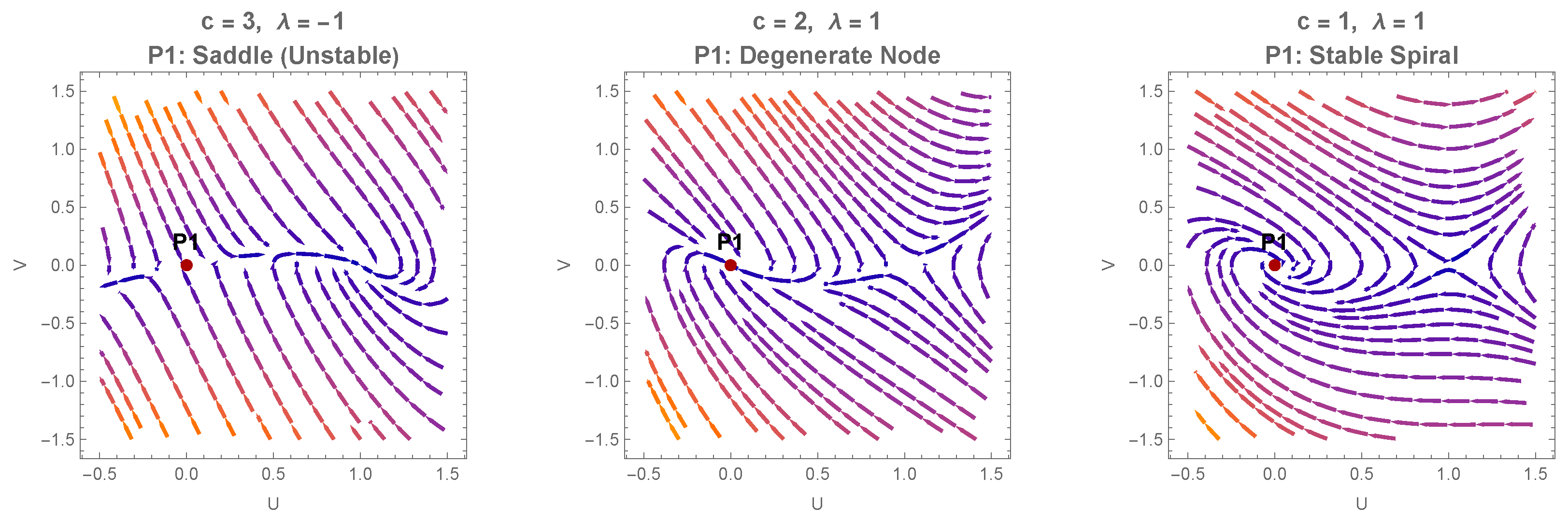
  • Case I: Saddle Point. For c = 3 and λ = 1 , we have c 2 = 9 > 4 λ = 4 . The critical points P 1 = ( 0 , 0 ) and P 2 = ( 1 , 0 ) yield Jacobians with real eigenvalues of opposite signs, indicating saddle points. Trajectories are repelled along unstable directions and attracted along stable ones. Both equilibria are thus unstable, meaning small perturbations lead the system away from the steady state, as presented in Figure 1.
  • Case II: Degenerate Node. For c = 2 , λ = 1 we have c 2 = 4 = 4 λ . At both critical points P 1 = ( 0 , 0 ) and P 2 = ( 1 , 0 ) , the Jacobian has a repeated real eigenvalue, indicating a degenerate node. Trajectories approach the equilibria in a directionally biased manner which maintains the stability, but convergence is weaker than in the spiral case.
  • Case III: Stable Spiral. For c = 1 , λ = 1 we have c 2 = 1 < 4 λ = 4 . The Jacobian at both P 1 = ( 0 , 0 ) and P 2 = ( 1 , 0 ) has complex eigenvalues with negative real parts, indicating stable spirals. Trajectories spiral inward toward the equilibria, reflecting damped oscillations commonly seen in physical systems.
Similarly, the ODE in Equation (58) can be rewritten as follows:
U = k 2 U 2 U + K e α y . α = c k 2
The dependence on variable y makes the ODE in Equation (58) a non-autonomous equation, which can be converted into an autonomous system by introducing a new variable defined by
Z ( y ) = e α y Z = α Z .
By changing the variable in the ODE in Equation (58), we obtain
U = k 2 U 2 U + K Z , where α = c k 2 . Z = α Z ,
From Z = α Z , this implies that Z = 0 as α 0 , and from U = 0 , we obtain
k 2 U 2 U = 0 U = 0 or U = 1 ( k 0 ) .
Thus, equilibria are
P 1 = ( 0 , 0 ) , P 2 = ( 1 , 0 ) ; ( α 0 , k 0 ) .
Consider
F ( U , Z ) = k 2 U 2 U + K Z , G ( U , Z ) = α Z .
The Jacobian matrix of the vector field ( F , G ) is given by
J ( U , Z ) = k 2 ( 2 U 1 ) K 0 α .
Since this matrix is upper triangular, its eigenvalues are given by its diagonal entries. We now evaluate J ( U , Z ) at the system equilibrium points. At the equilibrium point P 1 = ( 0 , 0 ) , we have
J ( 0 , 0 ) = k 2 K 0 α , μ 1 = k 2 , μ 2 = α .
At the equilibrium point P 2 = ( 1 , 0 ) , we obtain
J ( 1 , 0 ) = k 2 K 0 α , μ 1 = k 2 , μ 2 = α .
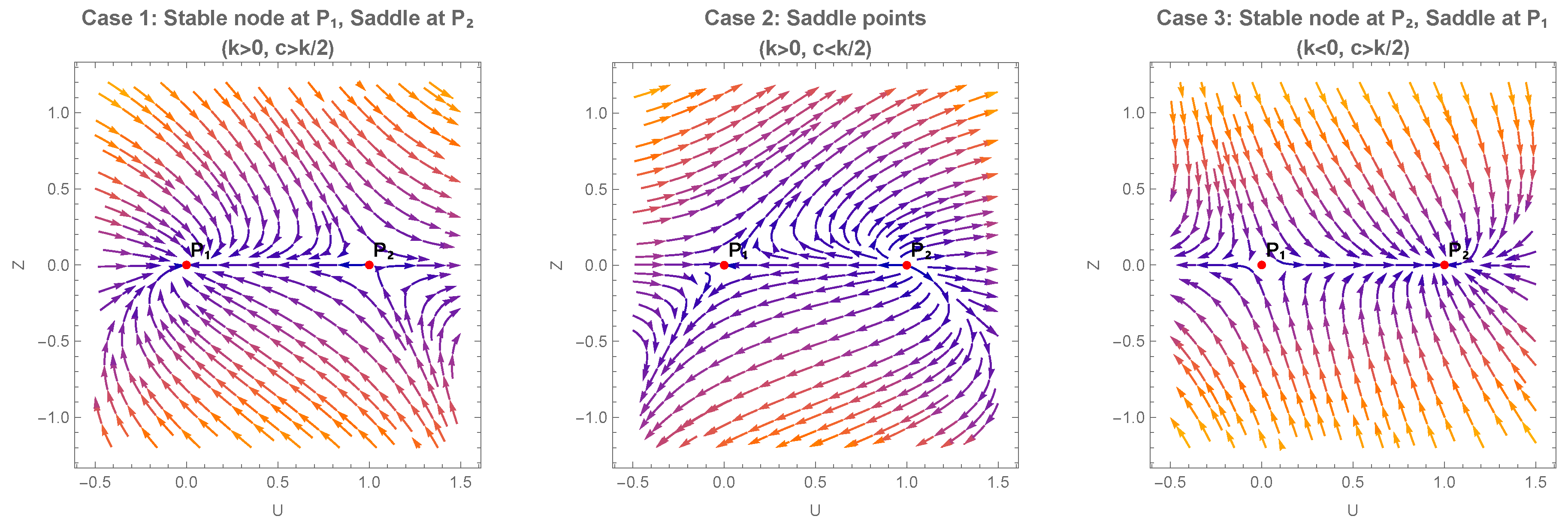
Since the eigenvalues of the Jacobian matrix associated with the system are real, the equilibrium point P 1 = ( 0 , 0 ) can only exhibit node or saddle behavior. By linearizing the system around P 1 , the eigenvalues are found to be μ 1 = k 2 and μ 2 = α , where α = c k 2 . The sign of these eigenvalues determines the stability of the equilibrium. If both μ 1 and μ 2 are negative with k > 0 and α > 0 , which implies c > k 2 , then P 1 is an asymptotically stable node. Conversely, if both eigenvalues are positive and corresponding to k < 0 and α < 0 or, equivalently, c < k 2 , then the equilibrium becomes an unstable node. When the eigenvalues have opposite signs where either ( k > 0 , α < 0 ) or ( k < 0 , α > 0 ) , then the equilibrium point P 1 behaves as a saddle point. These classifications are demonstrated in Figure 2.
The ODE in Equation (58) can be rewritten in a simpler notation:
U ( y ) + k 2 U ( y ) k 2 U ( y ) 2 = K e 1 2 ( 2 c k ) y , α : = c k 2 .
Equivalently, we have
U = k 2 U ( U 1 ) + K e α y .
For k 0 , the differential equation
U ( y ) = k 2 U ( U 1 ) + K e α y ,
is a Riccati equation, which has the general form
U ( y ) = a ( y ) + b U + c U 2 ,
with coefficients identified as follows:
a ( y ) = K e α y , b = k 2 , c = k 2 .
To solve Equation (77), we apply the standard substitution that transforms the Riccati equation into a linear second-order differential equation given by
U ( y ) = 1 c v ( y ) v ( y ) = 2 k v v .
Through substitution into Equation (77), we obtained the new function v ( y ) , which satisfies the linear second-order ODE
v + k 2 v + k K 2 e α y v = 0 .
Through a change of variables, this can be reduced to a simpler form by considering
t : = e α y / 2 . with α 0
This substitution maps the exponential dependence in y to an algebraic dependence in t, which is easier to handle. Next, we set
v ( y ) = t ν w ( t ) , where ν : = k α , λ : = 2 k K α .
With this ansatz, the equation for w ( t ) becomes the Bessel equation
t 2 w + t w + λ 2 t 2 ν 2 w = 0 .
This is a standard form whose general solution is given by a linear combination of Bessel functions of the first and second kind:
w ( t ) = C 1 J ν ( λ t ) + C 2 Y ν ( λ t ) .
Hence, the solution v ( y ) to the ODE in Equation (81) is
v ( y ) = t ν C 1 J ν ( λ t ) + C 2 Y ν ( λ t ) , with t = e α y / 2 .
Finally, from Equation (80), one convenient closed form for U can be obtained:
U ( y ) = α k ν + t w t ( t ) w ( t ) = 1 + α k t w t ( t ) w ( t ) , t = e α y / 2 ,
with w ( t ) = C 1 J ν ( λ t ) + C 2 Y ν ( λ t ) .
For complex λ , the Bessel functions J ν and Y ν are replaced by the modified Bessel functions I ν and K ν to represent exponential solutions. This transformation provides a closed-form representation of the solution to the Riccati equation via classical special functions.

4. The Direct Algebraic Method

  • Consider the fourth proposed model:
u x x + λ u λ u 2 u t k u u x = 0
A thorough description of the primary steps [24,25,26] involved in the EDAM is given in this section.
  • Step 1. Let us consider an NLPDE of the following form:
F ( w , w t , w x , w t t , w x x , ) = 0 .
By utilizing the transformation
w ( x , t ) = U ( ψ ) , ψ = x c t ,
where c 0 , we obtain an ordinary differential equation (ODE) of the form
G ( U , U , U , ) = 0 .
Step 2. We assume that the following solution of the ODE is
U = U ( ψ ) = j = 0 K a j Z j ( ψ ) ,
where a j ( j = 0 , 1 , 2 , K ) are constant coefficients to be found and Z ( ψ ) satisfies the ODE of the form
Z ( ψ ) = l n ( ρ ) χ + v W ( ψ ) + μ W 2 ( ψ ) , ρ 0 , 1 .
Here, v and χ , along with μ , are the real constants that can be seen in the auxiliary equation. The list of numerous solutions is given below.
  • Family-1: When ϕ < 0 and μ 0 , where ϕ = v 2 4 χ μ , we have
Z 1 ( ψ ) = v 2 μ + ϕ 2 μ tan ρ ϕ 2 ψ , Z 2 ( ψ ) = v 2 μ + ϕ 2 μ cot ρ ϕ 2 ψ , Z 3 ( ψ ) = v 2 μ + ϕ 2 μ tan ρ ϕ ψ ± g h sec ρ ϕ ψ , Z 4 ( ψ ) = v 2 μ + ϕ 2 μ cot ρ ϕ ψ ± g h csc ρ ϕ ψ , Z 5 ( ψ ) = v 2 μ + ϕ 4 μ tan ρ ϕ 4 ψ cot ρ ϕ 4 ψ .
Family-2: When ϕ > 0 and μ 0 , we have
Z 6 ( ψ ) = v 2 μ ϕ 2 μ tanh ρ ϕ 2 ( ψ ) , Z 7 ( ψ ) = v 2 μ ϕ 2 μ coth ρ ϕ 2 ( ψ ) , Z 8 ( ψ ) = v 2 μ + ϕ 2 μ tanh ρ ϕ ψ ± i g h sech ρ ϕ ψ , Z 9 ( ψ ) = v 2 μ + ϕ 2 μ coth ρ ϕ ψ ± i g h csch ρ ϕ ψ , Z 10 ( ψ ) = v 2 μ ϕ 4 μ tanh ρ ϕ 4 ψ coth ρ ϕ 4 ψ .
Family-3: When χ μ > 0 and v = 0 , we have
Z 11 ( ψ ) = χ μ tan ρ χ μ ψ , Z 12 ( ψ ) = χ μ cot ρ χ μ ψ , Z 13 ( ψ ) = χ μ tan ρ 2 χ μ ψ ± g h sec ρ 2 χ μ ψ , Z 14 ( ψ ) = χ μ cot ρ 2 χ μ ψ ± g h csc ρ 2 χ μ ψ , Z 15 ( ψ ) = 1 2 χ μ tan ρ χ μ 2 ψ cot χ μ 2 ψ .
Family-4: When χ μ < 0 and v = 0 , we have
Z 16 ( ψ ) = χ μ tanh ρ χ μ ψ , Z 17 ( ψ ) = χ μ coth ρ χ μ ψ , Z 18 ( ψ ) = χ μ tanh ρ 2 χ μ ψ ± i g h sech ρ 2 χ μ ψ , Z 19 ( ψ ) = χ μ coth ρ 2 χ μ ψ ± i g h csch ρ 2 χ μ ψ , Z 20 ( ψ ) = 1 2 χ μ tanh ρ χ μ 2 ψ + coth ρ χ μ 2 ψ .
Family-5: When v = 0 and χ = μ , we have
Z 21 ( ψ ) = tan ρ ( χ ( ψ ) ) , Z 22 ( ψ ) = cot ρ ( χ ( ψ ) ) , Z 23 ( ψ ) = tan ρ ( 2 χ ( ψ ) ) ± g h sec ρ ( 2 χ ψ ) , Z 24 ( ψ ) = cot ρ ( 2 χ ( ψ ) ) ± g h csc ρ ( 2 χ ψ ) , Z 25 ( ψ ) = 1 2 tan ρ χ 2 ψ cot ρ χ 2 ψ ,
Family-6: When v = 0 and χ = μ , we have
Z 26 ( ψ ) = tanh ρ ( χ ψ ) , Z 27 ( ψ ) = coth ρ ( χ ψ ) , Z 28 ( ψ ) = tanh ρ ( 2 χ ψ ) ± i g h sech ρ ( 2 χ ψ ) , Z 29 ( ψ ) = coth ρ ( 2 χ ψ ) ± g h csch ρ ( 2 χ ψ ) , Z 30 ( ψ ) = 1 2 tanh ρ ψ 2 χ + coth ρ ψ 2 χ .
Family-7: When v 2 = 4 χ μ , we have
Z 31 = 2 χ ( v ψ ln ρ + 2 ) v 2 ( ψ ) ln ρ .
Family-8: When v = p , χ = p q , ( q 0 ) and μ = 0 , we have
Z 32 = ρ p ( ψ ) q .
Family-9: When v = μ = 0 , we have
Z 33 = χ ( ψ ) ln ρ .
Family-10: When v = χ = 0 , we have
Z 34 ψ = 1 ζ ψ ln ρ .
Family-11: When χ = 0 and v 0 , we have
Z 35 = g v μ cosh ρ ( v ψ ) sinh ρ ( v ψ ) + g , Z 36 = v sinh ρ ( v ψ ) + cosh ρ ( v ψ ) μ sinh ρ ( v ψ ) + cosh ρ ( v ψ ) + h .
Family-12: When v = p and μ = p q , ( q 0 , χ = 0 ) , we have
Z 37 = g ρ p ψ g q h ρ p ψ .
Now, the hyperbolic and trigonometric functions are given as follows:
sinh ρ ( ψ ) = g ρ ψ h ρ ψ 2 , cosh ρ ( ψ ) = g ρ ψ + h ρ ψ 2 , tanh ρ ( ψ ) = g ρ ψ h ρ ψ g ρ ψ + h ρ ψ , coth ρ ( ψ ) = g ρ ψ + h ρ ψ g ρ ψ h ρ ψ , sech ρ ( ψ ) = 2 g ρ ψ + h ρ ψ , csch ρ ( ψ ) = 2 g ρ ψ h ρ ψ , sin ρ ( ψ ) = g ρ i ψ h ρ i ψ 2 i , cos ρ ( ψ ) = g ρ i ψ + h ρ i ψ 2 , tan ρ ( ψ ) = i g ρ i ψ h ρ i ψ g ρ i ψ + h ρ i ψ , cot ρ ( ψ ) = i g ρ i ψ + h ρ i ψ g ρ i ψ h ρ i ψ , sec ρ ( ψ ) = 2 g ρ i ψ + h ρ i ψ , csc ρ ( ψ ) = 2 i g ρ i ψ h ρ i ψ ,
where g , h > 0 are called parameters of deformation. By balancing the highest-order derivative term with the highest-order nonlinear term in Equation (89), we may find the value of K. The set of algebraic equations can be obtained by substituting Equation (91) and its necessary derivatives in Equation (89) and comparing the coefficients of power of Z ( ψ ) in the resulting equation.

Application of Analytical Technique

Let us take the transformation of the form
U ( x , t ) = U ( ψ ) , ψ = x c t ,
By using Equation (106) in Equation (87), we obtain the subsequent ODE:
u + c u k u u + μ u μ u 2 = 0 .
We acquire N = 2 by applying the homogeneous balancing method (HBM) between u 2 and u in Equation (107). For N = 2 , we have
U ( ψ ) = a 0 + a 1 Z ( ψ ) + a 2 Z ( ψ ) 2 ,
where a 0 , a 1 and a 2 are constants. The set of equations involving a 0 , a 1 and a 2 , as well as other parameters is obtained by summing up all the coefficients of distinct powers of Z ( ψ ) and combining Equations (108) and (92) with Equation (107). The following outcomes are obtained by solving these equations:
a 0 = 1 2 1 v v 2 4 χ μ , a 1 = μ v 2 4 χ μ , a 2 = 0 , k = 2 v 2 v 2 4 χ μ + 4 χ μ v 2 4 χ μ ,
c = v 2 v 2 4 χ μ 4 χ μ v 2 4 χ μ μ v 2 4 χ μ .
Accordingly, the solution to Equation (107), which corresponds to Equation (92), can be determined as follows.
  • Set 1: When ϕ < 0 and μ 0 , then
u 1 = 1 2 1 v v 2 4 χ μ μ v 2 4 χ μ ϕ tan ρ ϕ 2 ψ , u 2 = 1 2 1 v v 2 4 χ μ μ v 2 4 χ μ ϕ cot ρ ϕ 2 ψ , u 3 = 1 2 1 v v 2 4 χ μ μ v 2 4 χ μ ϕ tan ρ ϕ ψ ± g h sec ρ ϕ η , u 4 = 1 2 1 v v 2 4 χ μ μ v 2 4 χ μ ϕ cot ρ ϕ ψ ± g h csc ρ ϕ ψ , u 5 = 1 2 1 v v 2 4 χ μ μ v 2 4 χ μ ϕ 2 tan ρ ϕ 4 ψ cot ρ ϕ 4 ψ .
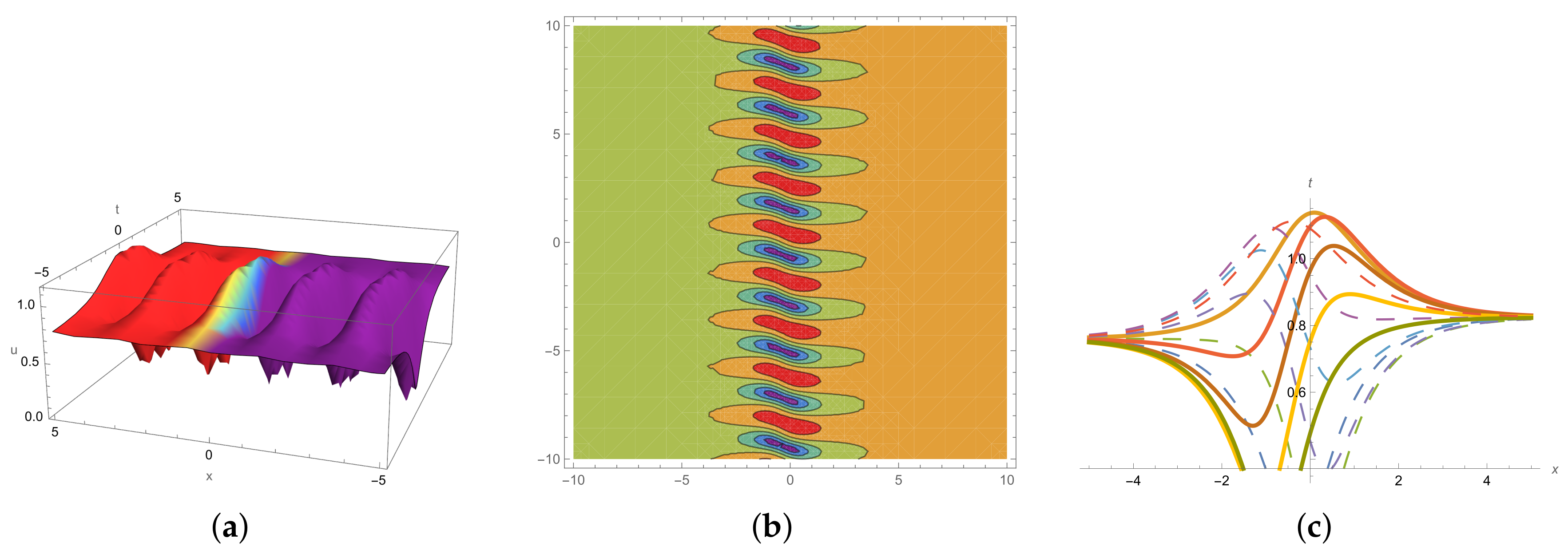
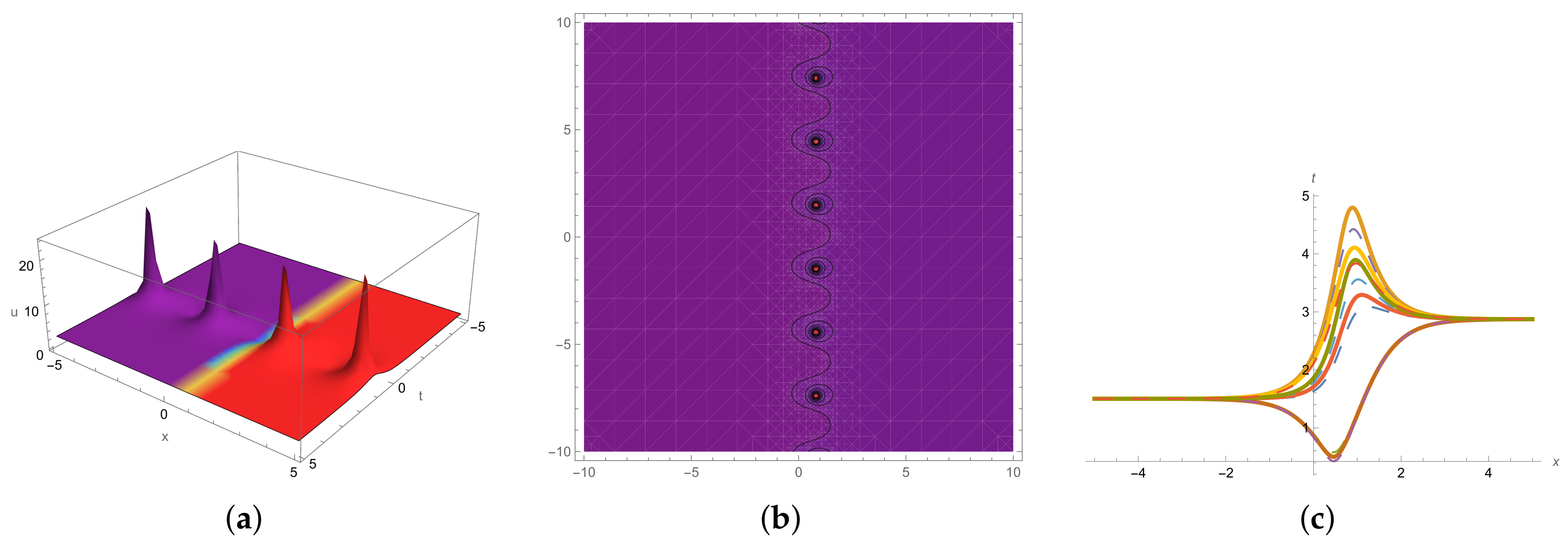
The solution u 1 and u 3 are displayed in Figure 3 and Figure 4 respectively.
  • Set-2: When ϕ > 0 and μ 0 , then
u 6 = 1 2 1 v v 2 4 χ μ μ v 2 4 χ μ ϕ tanh ρ ϕ 2 ψ , u 7 = 1 2 1 v v 2 4 χ μ μ v 2 4 χ μ ϕ coth ρ ϕ 2 ψ , u 8 = 1 2 1 v v 2 4 χ μ μ v 2 4 χ μ ϕ tanh ρ ϕ ψ ± i g h sech ρ ϕ ψ , u 9 = 1 2 1 v v 2 4 χ μ μ v 2 4 χ μ ϕ coth ρ ϕ ψ ± i g h csch ρ ϕ ψ , u 10 = 1 2 1 v v 2 4 χ μ μ v 2 4 χ μ ϕ 2 tanh ρ ϕ 4 ψ coth ρ ϕ 4 ψ .
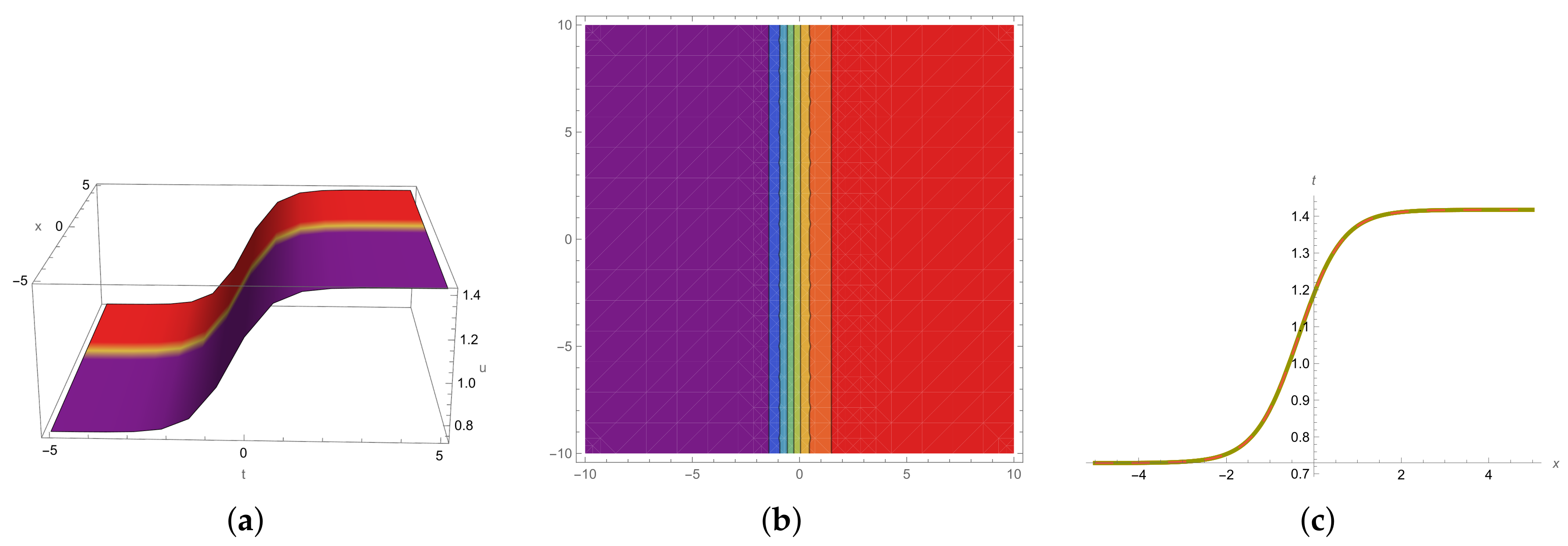
The solution u 6 and u 8 are displayed in Figure 5 and Figure 6 respectively.
  • Set-3: When χ μ > 0 and v = 0 , then
u 11 = 2 1 2 1 v v 2 4 χ μ μ v 2 4 χ μ χ μ tan ρ χ μ ψ , u 12 = 2 1 2 1 v v 2 4 χ μ μ v 2 4 χ μ χ μ cot ρ χ μ ψ , u 13 = 2 1 2 1 v v 2 4 χ μ μ v 2 4 χ μ χ μ tan ρ 2 χ μ ψ ± g h sec ρ 2 μ ζ η , u 14 = 2 1 2 1 v v 2 4 χ μ μ v 2 4 χ μ χ μ cot ρ 2 χ μ ψ ± g h csc ρ 2 χ μ ψ , u 15 = 1 2 1 v v 2 4 χ μ μ v 2 4 χ μ χ μ tan ρ χ μ 2 ψ cot χ μ 2 ψ .
Set-4: When χ μ < 0 and v = 0 , then
u 16 = 2 i 1 2 1 v v 2 4 χ μ μ v 2 4 χ μ χ μ tanh ρ χ μ ψ , u 17 = 2 i 1 2 1 v v 2 4 χ μ μ v 2 4 χ μ χ μ coth ρ χ μ ψ , u 18 = 2 i 1 2 1 v v 2 4 χ μ μ v 2 4 χ μ χ μ tanh ρ 2 χ μ ψ ± i g h sech ρ 2 χ μ ψ , u 19 = 2 i 1 2 1 v v 2 4 χ μ μ v 2 4 χ μ χ μ coth ρ 2 χ μ ψ ± i g h csch ρ 2 χ μ ψ , u 20 = 1 2 1 v v 2 4 χ μ μ v 2 4 χ μ i χ μ tanh ρ χ μ 2 ψ + coth ρ χ μ 2 ψ .
Set-5: When v = 0 and χ μ , then
u 21 = 2 1 2 1 v v 2 4 χ μ μ v 2 4 χ μ μ tan ρ ( χ ψ ) , u 22 = 2 1 2 1 v v 2 4 χ μ μ v 2 4 χ μ μ cot ρ ( χ ψ ) , u 23 = 2 1 2 1 v v 2 4 χ μ μ v 2 4 χ μ μ tan ρ ( 2 χ ψ ) ± g h sec ρ ( 2 χ ψ ) , u 24 = 2 1 2 1 v v 2 4 χ μ μ v 2 4 χ μ μ cot ρ ( 2 χ ψ ) ± g h csc ρ ( 2 χ ψ ) , u 25 = 1 2 1 v v 2 4 χ μ μ v 2 4 χ μ μ tan ρ χ 2 ψ cot ρ χ 2 ψ .
Set-6: When v = 0 and χ = μ , then
u 26 = 2 1 2 1 v v 2 4 χ μ μ v 2 4 χ μ μ tanh ρ ( χ ψ ) , u 27 = 2 Δ μ coth ρ ( χ ψ ) , u 28 = 2 1 2 1 v v 2 4 χ μ μ v 2 4 χ μ χ tanh ρ ( 2 χ ψ ) ± i g h sech ρ ( 2 χ ψ ) , u 29 = 2 1 2 1 v v 2 4 χ μ μ v 2 4 χ μ χ coth ρ ( 2 χ ψ ) ± i g h csch ρ ( 2 χ ψ ) , u 30 = 1 2 1 v v 2 4 χ μ μ v 2 4 χ μ χ tanh ρ χ 2 ψ ± coth ρ χ 2 ψ .
Set-7: When v 2 = 4 χ μ , then
u 31 = 1 v v 2 4 χ μ μ v 2 4 χ μ χ μ 1 χ μ 2 χ ( v ψ ln ρ + 2 ) v 2 ψ ln ρ .
Set-8: When v = δ = 0 , then
u 32 = 2 Δ ψ ln ρ .
Set-9: When χ = 0 and v 0 , then
u 33 = 1 2 1 v v 2 4 χ μ μ v 2 4 χ μ v 1 2 g cosh ρ ( v ψ ) sinh ρ ( v ψ ) + g , u 34 = 1 2 1 v v 2 4 χ μ μ v 2 4 χ μ v 1 2 sinh ρ ( v ψ ) + cosh ρ ( v ψ ) μ sinh ρ ( v ψ ) + cosh ρ ( v ψ ) + h .

5. Traveling Wave Solutions via Some Functional Transforms

The soliton solutions [27,28] are discussed [29,30] for partial differential equations (PDEs) that are nonlinear in the unknowns and their derivatives. A traveling wave solution [24,29,30,31] is an exact, closed-form solution expressed as a finite power series of one of a particular set of functions [29] (we consider tanh, sinh and cosh) that has a linear combination of the independent variables. Concretely, given such a PDE system with i unknown functions Z i ( x 1 , , x j ) of j variables, solutions take the form
Z i ( τ ) = k = 0 n i A i , k τ k ,
where the n i values are finite, the A i , k are constants with respect to x j and
τ = tanh ( k = 0 j c k x k ) ,
where c k represents the constants with respect to x j . Traveling wave solutions can be found by transforming the PDE system into a nonlinear ODE system by introducing τ as a new variable, implying
x j Z i = c j ( τ 2 + 1 ) ( τ Z i ) .
for all x j . The resulting ODE system, with the polynomial in Z i ( τ ) and its derivatives, has all the coefficients of the polynomial in τ and the unknowns c j . To search for solutions Z i = k = 0 n i A i , k τ k for that ODE system, an upper bound n i for each unknown Z i is computed. The complete finite expansion in τ for each Z i , containing the unknowns A i , k , is introduced in the ODE system obtained previously, and by taking coefficients of different powers of τ , a new algebraic nonlinear system for the expansion coefficients { A i , k , c j } is built and leads us to the solutions for A i , k in terms of c j . In the following sections, we present the soliton solutions for a second-order nonlinear nerve equation in bio-membranes with extension to fourth-order dispersion. Furthermore, one can also discuss the solutions of the forms not limited to
τ = sinh ( k = 0 j c k x k ) , τ = cosh ( k = 0 j c k x k ) , τ = sech ( k = 0 j c k x k ) ,
τ = sn k = 0 j c k x k , τ = cn k = 0 j c k x k , τ = dn k = 0 j c k x k , τ = ns k = 0 j c k x k , τ = nc k = 0 j c k x k , τ = nd k = 0 j c k x k .
In particular, for each case a transformation of the form
τ = f ( t · C [ 2 ] + x · C [ 1 ] + C [ 0 ] ) ,
is applied to reduce the PDE system into an ODE in terms of u ( τ ) . Then, a power series in τ is used to find the solution. The general form of the power series is
u ( τ ) = A [ 1 , 0 ] + A [ 1 , 1 ] · τ + A [ 1 , 2 ] · τ 2 + + A [ 1 , n ] · τ n ,
where the upper bound n depends on the function and structure of the reduced ODE.
For functions such as tan, tanh, cot, coth, sec, sech, csc and csch, the transformation yields ODEs that admit a linear power series with an upper bound n [ 1 ] = 1 presented in Table 1.

Traveling Wave Solutions and Applications

  • Traveling Wave Solutions: Family-I
  • When λ 0 and k 0 , the system admits two distinct families of exponential-type solutions. The first family involves pure exponential terms without constant shifts. These are given by
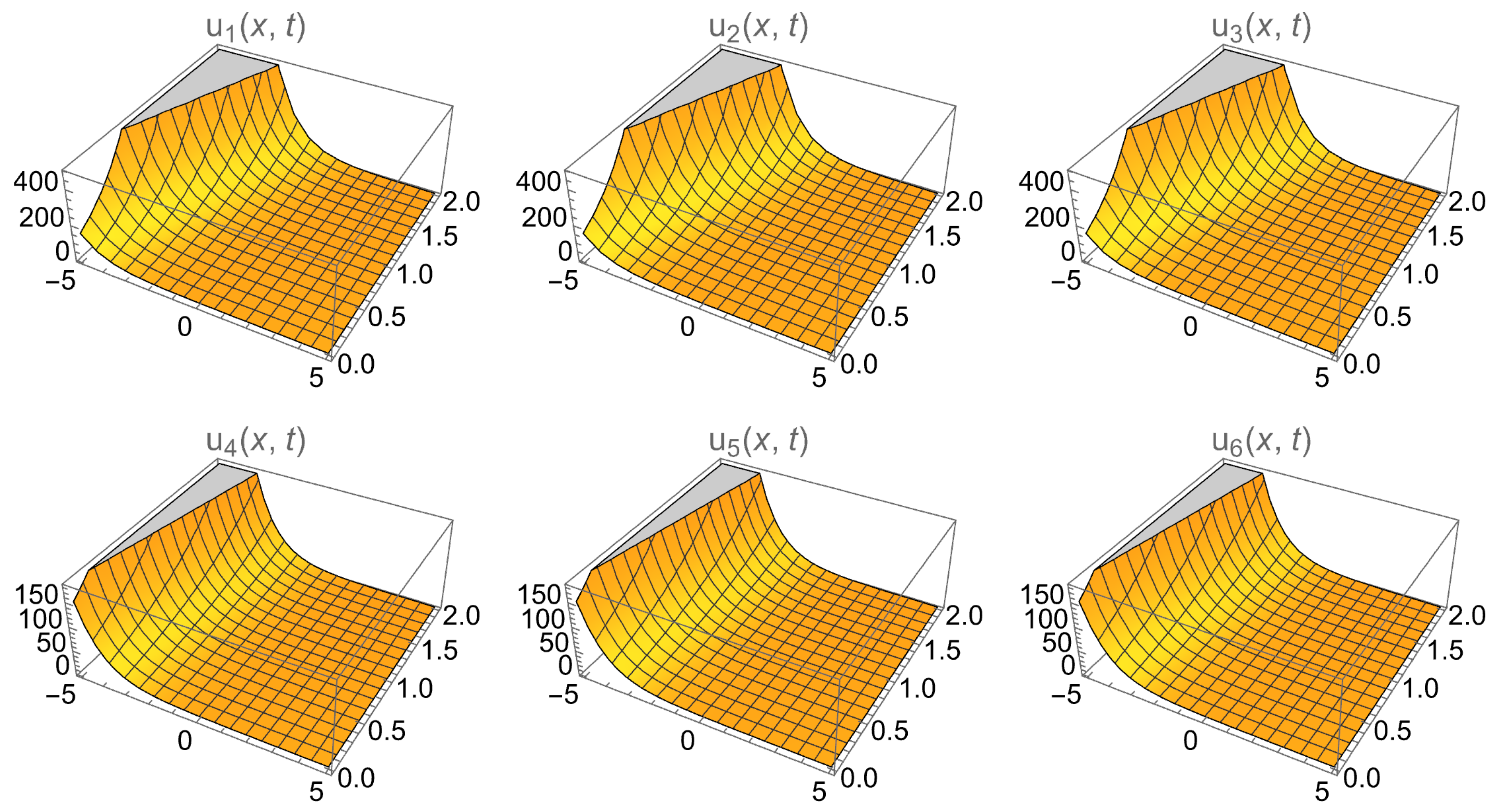
u 1 ( x , t ) = C 5 exp λ k 2 + λ k 2 t λ k x + C 1 , u 2 ( x , t ) = C 6 exp λ k 2 + λ 2 k 2 t λ 2 k x + C 1 2 , u 3 ( x , t ) = C 7 exp λ k 2 + λ 3 k 2 t λ 3 k x + C 1 3 ,
In contrast, the second family includes a constant shift of +1, modifying the long-term behavior of the solution
u 4 ( x , t ) = C 5 exp λ 2 k 2 t λ k x + C 1 + 1 , u 5 ( x , t ) = C 6 exp λ 2 2 k 2 t λ 2 k x + C 1 2 + 1 , u 6 ( x , t ) = C 7 exp λ 2 3 k 2 t λ 3 k x + C 1 3 + 1 .
These expressions describe exponential traveling wave solutions whose shape and growth depend on and are sensitive to parameters λ and k with or without the asymptotic shift presented in Figure 7.
  • Traveling Wave Solutions: Family-II
  • In the case where k = 0 and λ = 0 , the equation admits a family of exponential-type traveling wave solutions. The first-order solution is
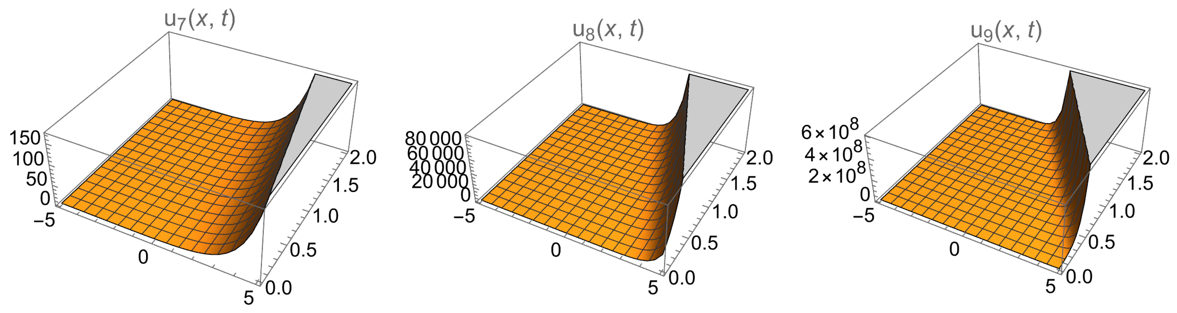
u 7 ( x , t ) = C 5 e C 2 2 t + C 2 x + C 1 + C 4 .
For the second order, the solution becomes
u 8 ( x , t ) = C 6 e 4 C 2 2 t + 2 C 2 x + 2 C 1 + C 4 .
The third-order solution takes the form
u 9 ( x , t ) = C 7 e 9 C 2 2 t + 3 C 2 x + 3 C 1 + C 4 .
This pattern extends naturally to higher orders, resulting in the general expression
u n ( x , t ) = C n + 4 e n 2 C 2 2 t + n C 2 x + n C 1 + C 4 , for n = 1 , 2 , 3 , .
These solutions describe exponentially growing wave profiles with both the growth rate and spatial steepness increasing with the order n, as presented in Figure 8.
  • Traveling Wave Solutions: Family-III
  • For the case λ = 0 , the PDE also admits several trigonometric and hyperbolic function solutions. These include
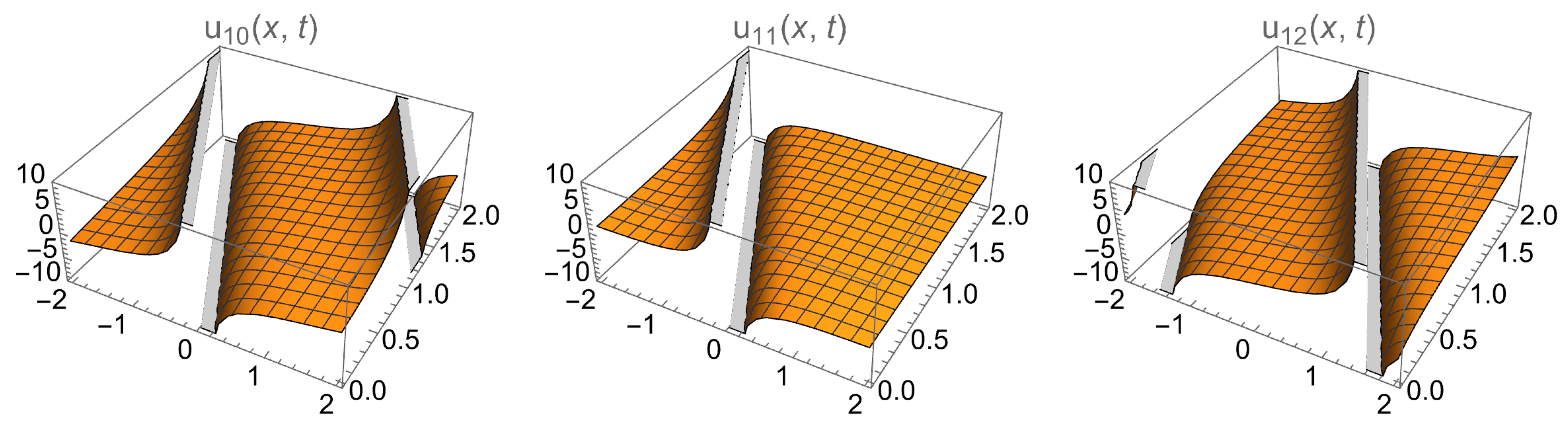
u 10 ( x , t ) = 2 C 2 k cot C 2 x + C 3 t + C 1 C 3 C 2 k , u 11 ( x , t ) = 2 C 2 k coth C 2 x + C 3 t + C 1 C 3 C 2 k , u 12 ( x , t ) = 2 C 2 k tan C 2 x + C 3 t + C 1 C 3 C 2 k , u 13 ( x , t ) = 2 C 2 k tanh C 2 x + C 3 t + C 1 C 3 C 2 k .
Each of these represents a wave-like solution whose form is governed by either a trigonometric or hyperbolic profile, depending on the specific choice, as presented in Figure 9.
  • Traveling Wave Solutions: Family-IV
  • For the case where λ = i 8 2 k 2 , several complex and real-valued solutions for u ( x , t ) arise involving both trigonometric and hyperbolic functions. These include
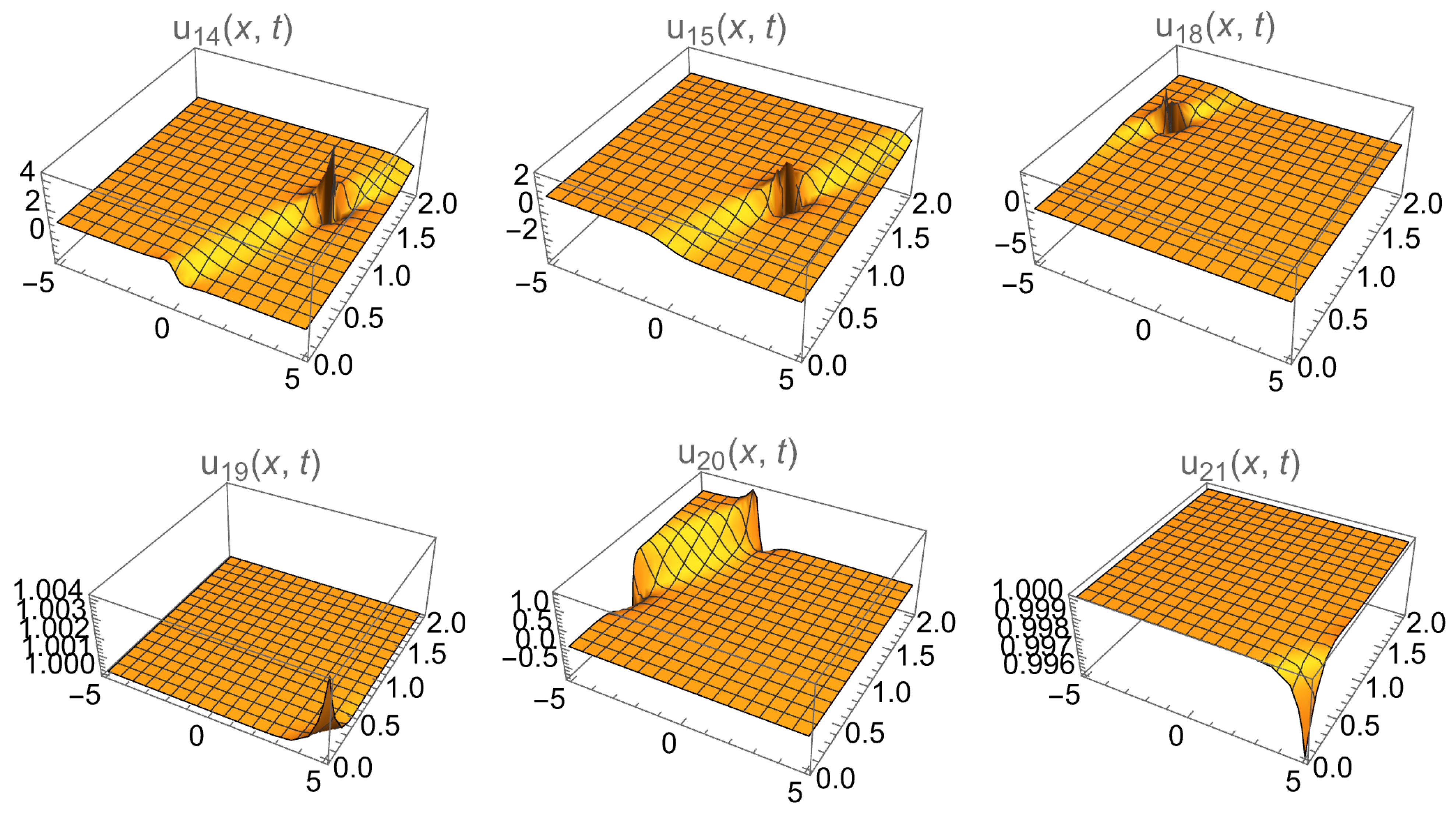
u 14 ( x , t ) = i 2 cot i 8 k 2 i 2 2 + 1 t + i 4 k x + C 1 + 1 2 , u 15 ( x , t ) = i 2 tan i 8 k 2 i 2 2 + 1 t i 4 k x + C 1 + 1 2 , u 16 ( x , t ) = i 2 cot i 8 k 2 i 2 2 + 1 t i 4 k x + C 1 + 1 2 , u 17 ( x , t ) = i 2 tan i 8 k 2 i 2 2 + 1 t + i 4 k x + C 1 + 1 2 , u 18 ( x , t ) = 1 2 coth 1 8 k 2 i 2 2 + 1 t + 1 4 k x + C 1 + 1 2 , u 19 ( x , t ) = 1 2 coth 1 8 k 2 i 2 2 + 1 t 1 4 k x + C 1 + 1 2 , u 20 ( x , t ) = 1 2 tanh 1 8 k 2 i 2 2 + 1 t + 1 4 k x + C 1 + 1 2 , u 21 ( x , t ) = 1 2 tanh 1 8 k 2 i 2 2 + 1 t 1 4 k x + C 1 + 1 2 .
These solutions reflect the interplay between complex parameters and real-valued output, giving rise to oscillatory or localized waveforms, depending on the function form and choice of constants, as presented in Figure 10.
  • Traveling Wave Solutions: Family-V
  • When λ = i 8 2 k 2 , a parallel set of complex and real-valued solutions for u ( x , t ) emerges. These take the form
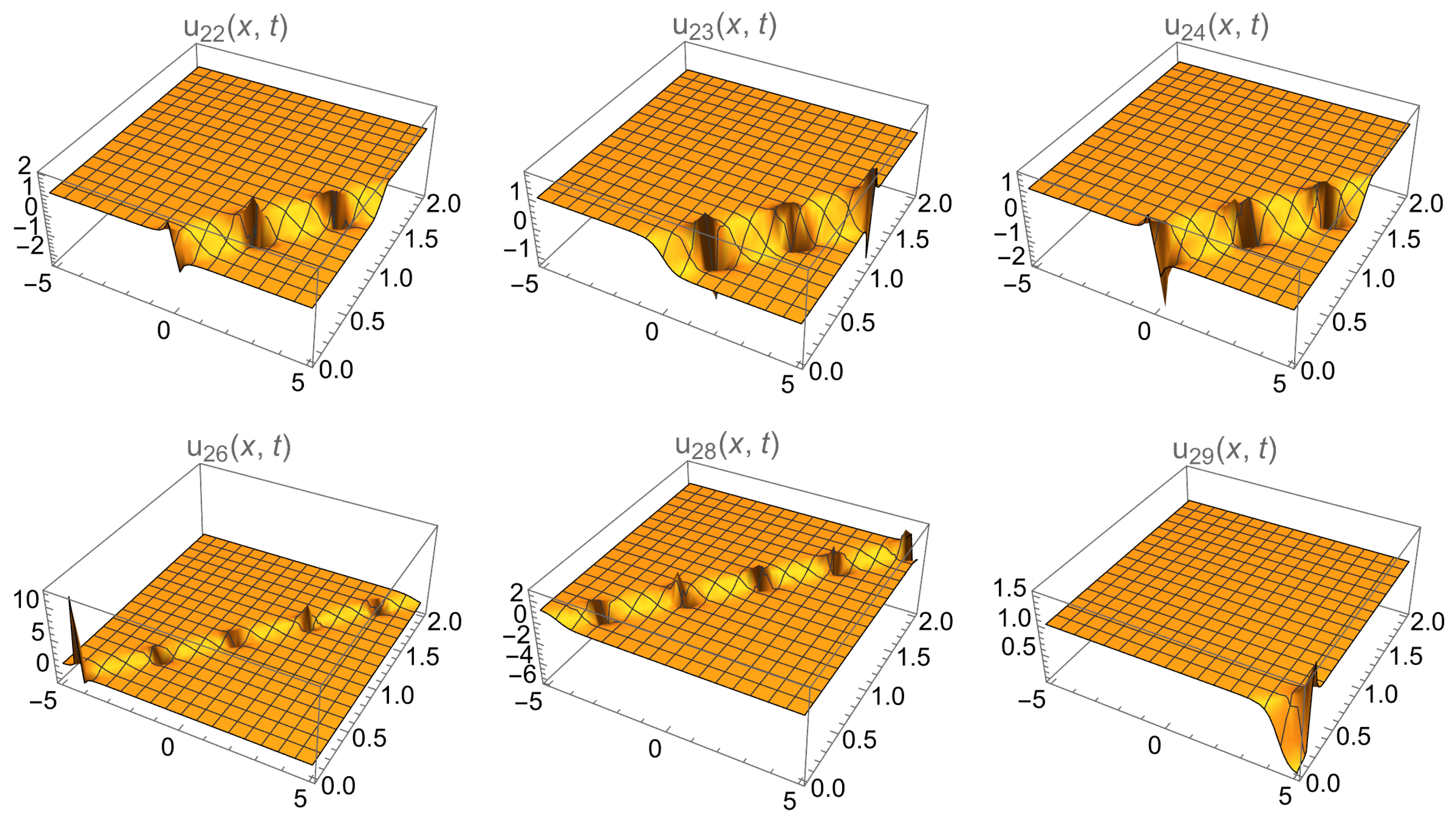
u 22 ( x , t ) = i 2 cot i 8 k 2 i 2 2 + 1 t + i 4 k x + C 1 + 1 2 , u 23 ( x , t ) = i 2 tan i 8 k 2 i 2 2 + 1 t i 4 k x + C 1 + 1 2 , u 24 ( x , t ) = i 2 cot i 8 k 2 i 2 2 + 1 t i 4 k x + C 1 + 1 2 , u 25 ( x , t ) = i 2 tan i 8 k 2 i 2 2 + 1 t + i 4 k x + C 1 + 1 2 , u 26 ( x , t ) = 1 2 coth 1 8 k 2 i 2 2 + 1 t + 1 4 k x + C 1 + 1 2 , u 27 ( x , t ) = 1 2 coth 1 8 k 2 i 2 2 + 1 t 1 4 k x + C 1 + 1 2 , u 28 ( x , t ) = 1 2 tanh 1 8 k 2 i 2 2 + 1 t + 1 4 k x + C 1 + 1 2 , u 29 ( x , t ) = 1 2 tanh 1 8 k 2 i 2 2 + 1 t 1 4 k x + C 1 + 1 2 .
As with the previous case, these solutions capture a variety of waveforms—some complex-valued some real—depending on the function type and the specific argument structure. They reflect the effect of a purely imaginary parameter λ on the phase and evolution of the wave, as presented in Figure 11.
  • Traveling Wave Solutions: Family-VI
  • When λ = 1 4 k 2 ± 2 C 3 , real-valued solutions for u ( x , t ) can be expressed using hyperbolic functions. For the case where λ = 1 4 k 2 2 C 3 , the solutions take the form
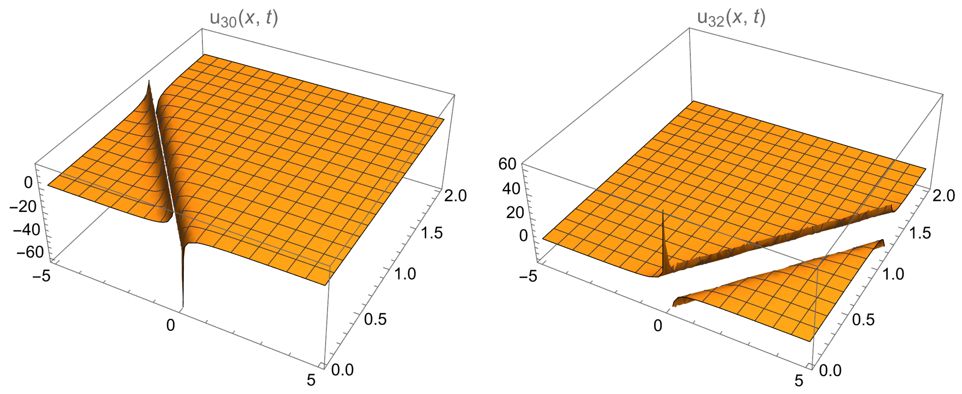
u 30 ( x , t ) = 1 2 coth C 3 t + 1 4 k x + C 1 + 1 2 , u 31 ( x , t ) = 1 2 tanh C 3 t + 1 4 k x + C 1 + 1 2 .
In contrast, for λ = 1 4 k 2 + 2 C 3 , the corresponding solutions are
u 32 ( x , t ) = 1 2 coth C 3 t 1 4 k x + C 1 + 1 2 , u 33 ( x , t ) = 1 2 tanh C 3 t 1 4 k x + C 1 + 1 2 .
These solutions exhibit either sharp wavefronts or smooth localized transitions, depending on the sign and type of the hyperbolic function, as presented in Figure 12.

6. Conclusions

We studied, in detail, the classical Fisher–Kolmogorov equation, which demonstrates how the combination of nonlinear reaction dynamics and diffusion gives rise to stable traveling wavefronts that propagate at a constant speed while preserving their shape. We adopted a number of approaches in dealing with the analyses: symmetry and invariance methods, conservation laws, solitons and Painlev’e analysis, among others. Detailed graphical representations were given.

Author Contributions

Conceptualization, A.R. and A.M.A.A.; methodology, A.M.A.A.; software, A.H.K.; validation, A.H.K., A.R. and A.M.A.A.; formal analysis, A.R.; investigation, A.M.A.A.; resources, A.M.A.A.; data curation, A.M.A.A.; original draft preparation writing, A.R.; review and editing of the original manuscript, A.R.; visualization, A.R.; supervision, A.R. and A.H.K.; project administration, A.H.K.; funding acquisition, A.R. All authors have read and agreed to the published version of the manuscript.

Funding

This research received no external funding.

Institutional Review Board Statement

Not applicable.

Informed Consent Statement

Not applicable.

Data Availability Statement

Data were not used to support the findings of this study.

Conflicts of Interest

The authors declare that there are no conflicts of interest of any form.

References

  1. Rothemund, P.W.; Winfree, E. The program-size complexity of self-assembled squares. In Proceedings of the Thirty-Second Annual ACM Symposium on Theory of Computing, Portland, OR, USA, 21–23 May 2000; pp. 459–468. [Google Scholar]
  2. Segel, L.A. (Ed.) Mathematical Models in Molecular Cellular Biology; CUP Archive: Cambridge, UK, 1980. [Google Scholar]
  3. Fife, P.C. Long time behavior of solutions of bistable nonlinear diffusion equations. Arch. Ration. Mech. Anal. 1979, 70, 31–36. [Google Scholar] [CrossRef]
  4. Britton, N.F. Reaction-Diffusion Equations and Their Applications to Biology; Academic Press: London, UK, 1986. [Google Scholar]
  5. Kareiva, P.M. Local movement in herbivorous insects: Applying a passive diffusion model to mark-recapture field experiments. Oecologia 1983, 57, 322–327. [Google Scholar] [CrossRef] [PubMed]
  6. Wang, G.; Tan, Z.; Gao, X.Y.; Liu, J.G. A new (2+1)-dimensional like-Harry-Dym equation with derivation and soliton solutions. Appl. Math. Lett. 2025, 172, 109720. [Google Scholar] [CrossRef]
  7. Zhang, H.; Wang, Z. Optimal system, invariant solutions and conservation laws of the hyperbolic geometry flow with time-dependent dissipation. J. Geom. Phys. 2023, 183, 104702. [Google Scholar] [CrossRef]
  8. Liu, X.; Yang, Z.W. Numerical analysis of a reaction–diffusion susceptible–infected–susceptible epidemic model. Comput. Appl. Math. 2022, 41, 392. [Google Scholar] [CrossRef]
  9. Li, W.; Liu, X.; Lang, Y. Numerical analysis of a nonlinear age-structured HBV model with saturated incidence and spatial diffusion. Math. Comput. Simul. 2024, 225, 250–266. [Google Scholar] [CrossRef]
  10. Olver, P.J. Applications of Lie Groups to Differential Equations; Springer Science & Business Media: Berlin/Heidelberg, Germany, 1993. [Google Scholar]
  11. Bluman, G.; Kumei, S. Symmetries and Differential Equations; Springer Science & Business Media: Berlin/Heidelberg, Germany, 2013. [Google Scholar]
  12. Bluman, G.; Anco, S.C. Symmetry and Integration Methods for Differential Equations; Springer: New York, NY, USA, 2002. [Google Scholar]
  13. Stephani, H. Differential Equations: Their Solution Using Symmetries; Cambridge University Press: Cambridge, UK, 1989. [Google Scholar]
  14. Ibragimov, N.H. Transformation Groups Applied to Mathematical Physics; Springer Science & Business Media: Berlin/Heidelberg, Germany, 1984. [Google Scholar]
  15. Ibragimov, N.H. CRC Handbook of Lie Group Analysis of Differential Equations; CRC press: Boca Raton, FL, USA, 2024; Volume III. [Google Scholar]
  16. Rafiq, M.H.; Jhangeer, A.; Raza, N. Symmetry and complexity: A Lie symmetry approach to bifurcation, chaos, stability and travelling wave solutions of the (3+1)-dimensional Kadomtsev–Petviashvili equation. Phys. Scr. 2023, 98, 115239. [Google Scholar] [CrossRef]
  17. Kara, A.H.; Mahomed, F.M. A Basis of Conservation Laws for Partial Differential Equations. J. Nonlinear Math. Phys. 2002, 9, 60–72. [Google Scholar] [CrossRef]
  18. Kara, A.H.; Mahomed, F.M. Relationship Between Symmetries and Conservation Laws. Int. J. Theor. Phys. 2000, 39, 23–40. [Google Scholar] [CrossRef]
  19. Bokhari, A.H.; Kara, A.H.; Zaman, F.D. A note on symmetry analyis and exact. Appl. Math. Lett. 2006, 19, 1356. [Google Scholar]
  20. Kara, A.H.; Khalique, C.M. Nonlinear evolution-type equations and their exact solutions using inverse variational methods. J. Phys. A Math. Gen. 2005, 38, 4629. [Google Scholar] [CrossRef]
  21. Ahmed, M.M.; Kara, A.H. Painlevé properties, gauge invariance and solitons of some classes of reaction-diffusion equations. Chaos Solitons Fractals 2021, 153, 111589. [Google Scholar] [CrossRef]
  22. Anco, S.C.; Bluman, G. Direct construction method for conservation laws of partial differential equations Part I: Examples of conservation law classifications. Eur. J. Appl. Math. 2002, 13, 545–566. [Google Scholar] [CrossRef]
  23. Kara, A.H. On the relationship between the invariance and conservation laws of differential equations. J. Math. 2018, 1, 2952583. [Google Scholar] [CrossRef]
  24. Pandit, S. A new algorithm for analysis and simulation of (2+1) Korteweg–de Vries–Rosenau-regularized long-wave model. Comput. Appl. Math. 2024, 43, 35. [Google Scholar] [CrossRef]
  25. Raza, N.; Rafiq, M.H.; Bekir, A.; Rezazadeh, H. Optical solitons related to (2+1)-dimensional Kundu–Mukherjee–Naskar model using an innovative integration architecture. J. Nonlinear Opt. Phys. Mater. 2022, 31, 2250014. [Google Scholar] [CrossRef]
  26. Javid, A.; Seadawy, A.R.; Raza, N. Dual-wave of resonant nonlinear Schrödinger’s dynamical equation with different nonlinearities. Phys. Lett. A 2021, 407, 127446. [Google Scholar] [CrossRef]
  27. Ablowitz, M.J.; Clarkson, P.A. Solitons, Nonlinear Evolution Equations and Inverse Scattering; Cambridge University Press: Cambridge, UK, 1991; Volume 149. [Google Scholar]
  28. Ma, W.X. Interaction solutions to Hirota–Satsuma–Ito equation in (2+1)-dimensions. Front. Math. China 2019, 14, 619–629. [Google Scholar] [CrossRef]
  29. Prado, H.P.; Cisneros-Ake, L.A. Alternative solitons in the Hirota–Satsuma system via the direct method. Partial. Differ. Equ. Appl. Math. 2021, 3, 100020. [Google Scholar] [CrossRef]
  30. Malwe, B.H.; Betchewe, G.; Doka, S.Y.; Kofane, T.C. Travelling wave solutions and soliton solutions for the nonlinear transmission line using the generalized Riccati equation mapping method. Nonlinear Dyn. 2016, 84, 171–177. [Google Scholar] [CrossRef]
  31. Jiwari, R.; Kumar, V.; Singh, S. Lie group analysis, exact solutions and conservation laws to compressible isentropic Navier–Stokes equation. Eng. Comput. 2022, 38, 2027–2036. [Google Scholar] [CrossRef]
Figure 1. Phase portraits of the dynamical system for three characteristic cases based on the parameter c = 1 , 2 , 3 with fixed λ = 1 .
Symmetry 18 00377 g001
Figure 2. Phase portraits illustrating the stability of the equilibrium points P 1 = ( 0 , 0 ) and P 2 = ( 1 , 0 ) under a varying parameter k and c.
Symmetry 18 00377 g002
Figure 3. The wave profile representing the multiple bright soliton solution for u 1 : (a) 3D plot, (b) contour plot, and (c) 2D plot when χ = 5 , v = 2 , μ = 5 , λ = 1 , m = 1 , n = 5 .
Symmetry 18 00377 g003
Figure 4. The wave profile of the periodic soliton solution for u 3 : (a) 3D plot, (b) contour plot, and (c) 2D plot when χ = 5 , v = 2 , μ = 5 , λ = 1 , m = 1 , n = 5 .
Symmetry 18 00377 g004
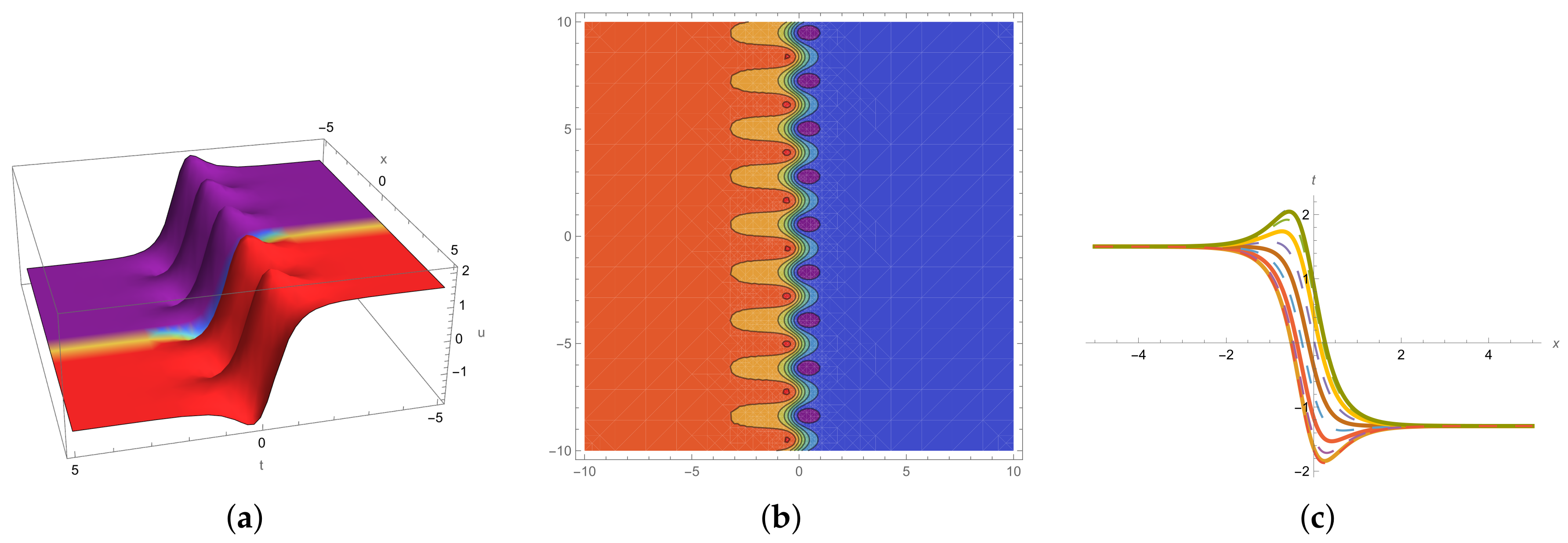
Figure 5. The wave profile representing the kink soliton solution for u 6 : (a) 3D plot, (b) contour plot, and (c) 2D plot when χ = 5 , v = 2 , μ = 5 , λ = 1 , m = 1 , n = 5 .
Symmetry 18 00377 g005
Figure 6. The wave profile representing anti-kink soliton solution for u 8 , (a) 3D plot, (b) contour plot, (c) 2D plot, when χ = 5 , v = 2 , μ = 5 , λ = 1 , m = 1 , n = 5 .
Symmetry 18 00377 g006
Figure 7. Surface plots of solutions u i ( x , t ) (for i = 1 , , 6 ).
Symmetry 18 00377 g007
Figure 8. 3D plots of solutions u 7 ( x , t ) , u 8 ( x , t ) and u 9 ( x , t ) .
Symmetry 18 00377 g008
Figure 9. 3D plots of solutions u 10 ( x , t ) , u 11 ( x , t ) and u 12 ( x , t ) .
Symmetry 18 00377 g009
Figure 10. 3D plots of solutions u 14 ( x , t ) , u 15 ( x , t ) , u 18 ( x , t ) , u 19 ( x , t ) , u 20 ( x , t ) and u 21 ( x , t ) .
Symmetry 18 00377 g010
Figure 11. 3D plots of solutions u 22 ( x , t ) , u 23 ( x , t ) , u 24 ( x , t ) , u 26 ( x , t ) , u 28 ( x , t ) and u 29 ( x , t ) .
Symmetry 18 00377 g011
Figure 12. 3D plots of solutions u 30 ( x , t ) and u 32 ( x , t ) .
Symmetry 18 00377 g012
Table 1. Power Series Reduction for Trigonometric and Hyperbolic Cases.
FunctionTransformation τ = f ( · ) Power Series SolutionParameter Splitting
cot cot ( t C [ 2 ] + x C [ 1 ] + C [ 0 ] ) u ( τ ) = A 1 , 0 + A 1 , 1 · τ { k , λ }
coth coth ( t C [ 2 ] + x C [ 1 ] + C [ 0 ] ) u ( τ ) = A 1 , 0 + A 1 , 1 · τ { k , λ }
csc csc ( t C [ 2 ] + x C [ 1 ] + C [ 0 ] ) u ( τ ) = A 1 , 0 + A 1 , 1 · τ { k , λ }
csch csch ( t C [ 2 ] + x C [ 1 ] + C [ 0 ] ) u ( τ ) = A 1 , 0 + A 1 , 1 · τ { k , λ }
sec sec ( t C [ 2 ] + x C [ 1 ] + C [ 0 ] ) u ( τ ) = A 1 , 0 + A 1 , 1 · τ { k , λ }
sech sech ( t C [ 2 ] + x C [ 1 ] + C [ 0 ] ) u ( τ ) = A 1 , 0 + A 1 , 1 · τ { k , λ }
tan tan ( t C [ 2 ] + x C [ 1 ] + C [ 0 ] ) u ( τ ) = A 1 , 0 + A 1 , 1 · τ { k , λ }
tanh tanh ( t C [ 2 ] + x C [ 1 ] + C [ 0 ] ) u ( τ ) = A 1 , 0 + A 1 , 1 · τ { k , λ }
Disclaimer/Publisher’s Note: The statements, opinions and data contained in all publications are solely those of the individual author(s) and contributor(s) and not of MDPI and/or the editor(s). MDPI and/or the editor(s) disclaim responsibility for any injury to people or property resulting from any ideas, methods, instructions or products referred to in the content.