Intelligent Mine Ventilation Systems

Abstract

The article discusses the development and design of intelligent mine ventilation systems, which are an important part of the construction and modernization of modern mines, as well as key technical support for the implementation of intelligent mining technologies. A high-fidelity simulation environment is constructed using neural networks based on field data. In the process of mine ventilation control, due to the complexity of the tunnel environment, it is difficult to investigate the implicit relationship between the ventilation system outlet control parameters and the concentration of gas and dust, oxygen, and carbon dioxide in the tunnel. Hence, it is difficult to obtain an overall control strategy based on experience. This article explores the possibility of applying reinforcement learning to intelligent shaft ventilation systems, a dynamic process in which model parameters, such as strategies and value functions, are updated through continuous interaction with the environment.

1. Introduction

The properties of symmetric control systems are considered; their distinctive feature is that the solution of the optimal control problem for an object whose mathematical model belongs to this class leads to the solution of two problems. Let us consider symmetric systems in the context of an optimal control problem and present a general formulation.

The mine ventilation system serves as critical infrastructure for ensuring safe and efficient mining production. Its primary function is to continuously supply adequate fresh air to underground working spaces, diluting and removing harmful substances such as gas and dust, and regulating the environmental climate. As mining extends to deeper, more complex conditions, the traditional ventilation control model, which relies on static models and manual experience, has become increasingly inadequate at adapting to dynamically changing mining environments. This results in issues such as delayed adjustments, high energy consumption, and significant safety risks. Therefore, the development of intelligent, adaptive ventilation control technologies has become a core requirement for modernizing mining operations.

As part of the modernization and construction of modern mines, a reversible process for controlling the main fan’s operation using an anti-icing damper is proposed [1], and the heat transfer effects of various shunt structures are also being modeled. ZHOU et al. [2] present a cloud-based platform for real-time monitoring and intelligent optimization of ventilation parameters. Xu et al. [3] propose a method for monitoring and optimizing ventilation parameters and tracking ventilation system malfunctions based on a 3D monitoring model. In Zhang et al. [4] an intelligent wind flow detection model for metal mines based on the CNN-LSTM architecture is built using deep-learning methods, the method of inversion of the mine ventilation resistance coefficient based on a genetic algorithm is investigated [5], a new method for controlling local ventilation is proposed [6] to achieve accurate control of airflow by optimizing the operating parameters of the local fan, which improves the efficiency and safety of the local ventilation system. Ventilation.

Among numerous studies in the literature, it has been proposed to apply the deep Q-network algorithm (DQN) in reinforcement learning for an intelligent mine ventilation system. However, existing research predominantly relies on static models or traditional control methods, which struggle to adapt to the dynamic, multi-parameter, and coupled environment of mine ventilation in real time. To address this gap, this paper proposes applying a Deep Q-Network (DQN) algorithm for dynamic control of ventilation louvers. The key innovations of this study are: It is among the first to apply DQN specifically to the real-time angle control of ventilation louvers in a mine return airway; It provides a comparative analysis demonstrating DQN’s superiority over baseline methods in terms of cumulative reward, convergence speed, and control stability; It establishes a complete simulation environment integrating computational fluid dynamics (CFD), a BP neural network surrogate model, and the DQN algorithm to form a closed-loop intelligent control framework. This method enables adaptive adjustment of the ventilation strategy by intelligently learning and optimizing the operating status of the ventilation system.

In addition, with the rapid development of sensing technology and the industrial Internet of Things (IIoT), heterogeneous multi-source data, such as airflow velocity, gas concentration, equipment operating status, and environmental parameters, can be continuously collected from underground ventilation systems. These data provide a foundation for intelligent analysis and decision-making, but also pose challenges due to their high dimensionality, strong coupling, and dynamic uncertainty. Traditional rule-based or model-based control methods rely heavily on simplified assumptions and empirical parameter tuning, making it difficult to achieve optimal ventilation control under complex, time-varying underground conditions.

To address these challenges, data-driven methods have gradually attracted attention in the field of mine ventilation. Machine-learning and deep-learning techniques have been applied to ventilation parameter prediction, fault diagnosis, and airflow distribution analysis, demonstrating improved accuracy compared with conventional approaches. However, most existing methods focus on offline modeling or static optimization and lack the capability of real-time adaptive control. In practical applications, the ventilation environment is continuously changing due to mining activities, equipment operation, and geological conditions, which requires the control strategy to dynamically adjust in response to environmental feedback.

Reinforcement learning provides a promising framework for solving such sequential decision-making problems under uncertainty. By interacting with the ventilation environment and receiving feedback in the form of rewards, an intelligent agent can learn an optimal control policy without relying on an explicit mathematical model of the system. Compared with supervised learning methods, reinforcement learning is better suited to ventilation control scenarios where labeled data are scarce and system dynamics are difficult to model accurately. Therefore, integrating reinforcement-learning algorithms into intelligent mine ventilation systems has the potential to improve system adaptability, safety, and energy efficiency.

The main contributions of this work are as follows: By combining computational fluid dynamics analysis, system identification, and field data, a high-fidelity and interactive ventilation simulation environment based on neural networks was constructed; A Deep Q-Network (DQN) algorithm tailored for mine ventilation control was designed, with explicit definitions of its states, actions, and reward functions; A comprehensive study covering environment modeling, algorithm training, and strategy verification was completed. Simulation results demonstrate that the proposed method effectively optimizes roadway environmental parameters and enhances the safety and adaptability of the ventilation system.

2. Materials and Methods

2.1. Window Geometry Model and Mesh Splitting

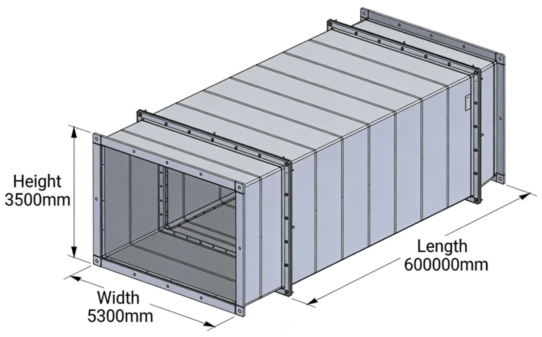
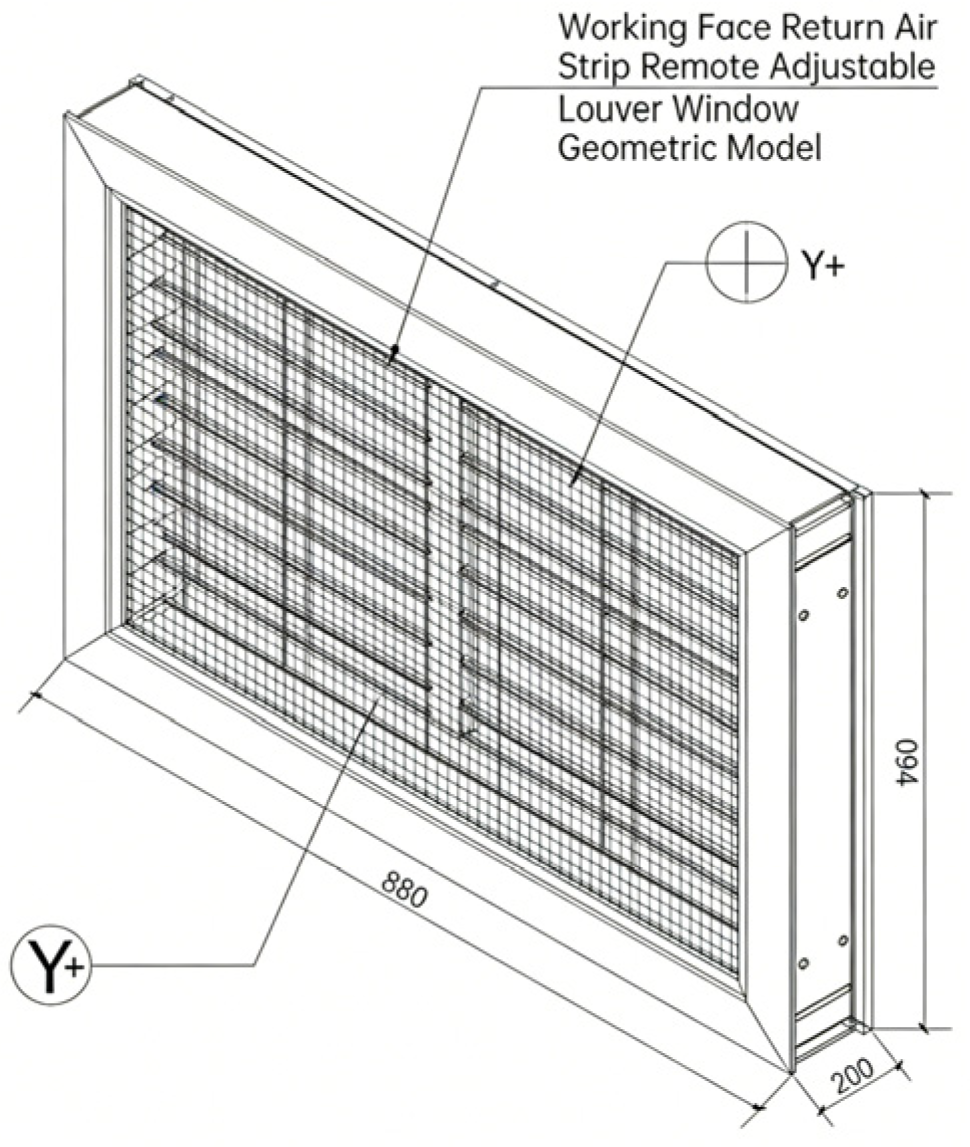
In this work, the actual dimensions of the remote adjustable louvered wind windows in the return air strip of the working surface are established in accordance with

Table 1. Specific parameters of culvert and window models.

Name	Size/mm	Name	Size/mm
Width of the carriageway	5300	Roadway height	3500
Length of the carriageway	600,000	Window width	3650
Window height	2550	Window thickness	200
Length of a one-page canvas	3650	Width of single-sheet blades	170

.

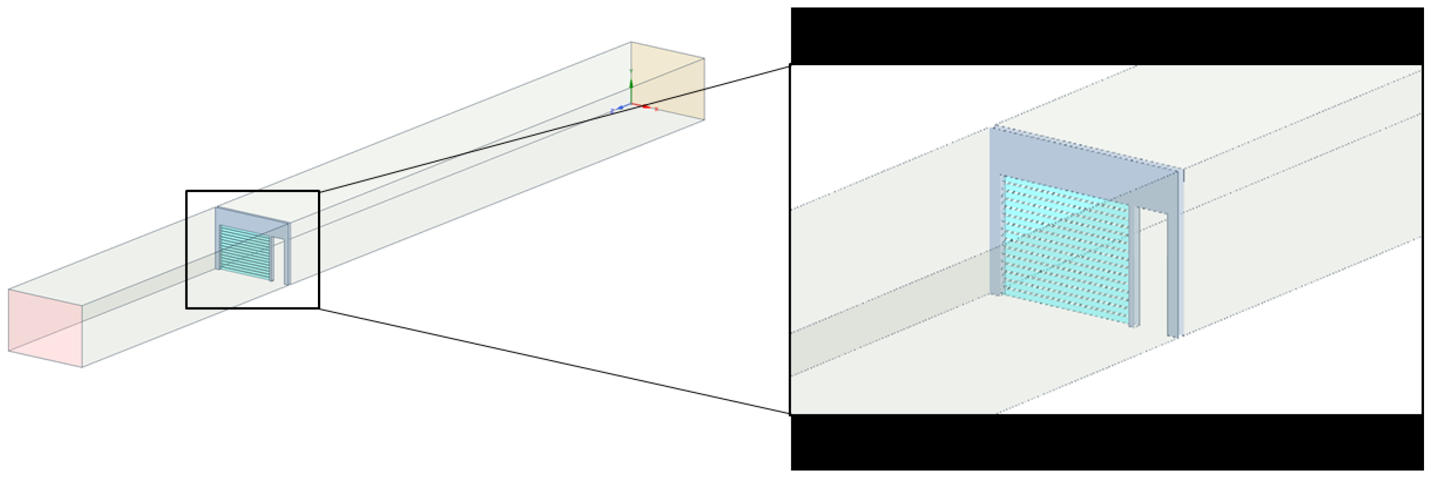
In the Figure 1 and Figure 2 the model is hooked with Fluent Meshing with Poly-Hexcore separation and boundary layers for strips and blade surfaces. Boundary conditions were set as follows: inlet as velocity inlet (1.5 m/s), outlet as pressure outlet, and walls as no-slip boundaries. The tunnel length was set to 60 m to ensure a fully developed flow downstream of the window, with vortex zones stabilized within this distance, thereby not affecting upstream monitoring.

2.1.1. Speed Distribution

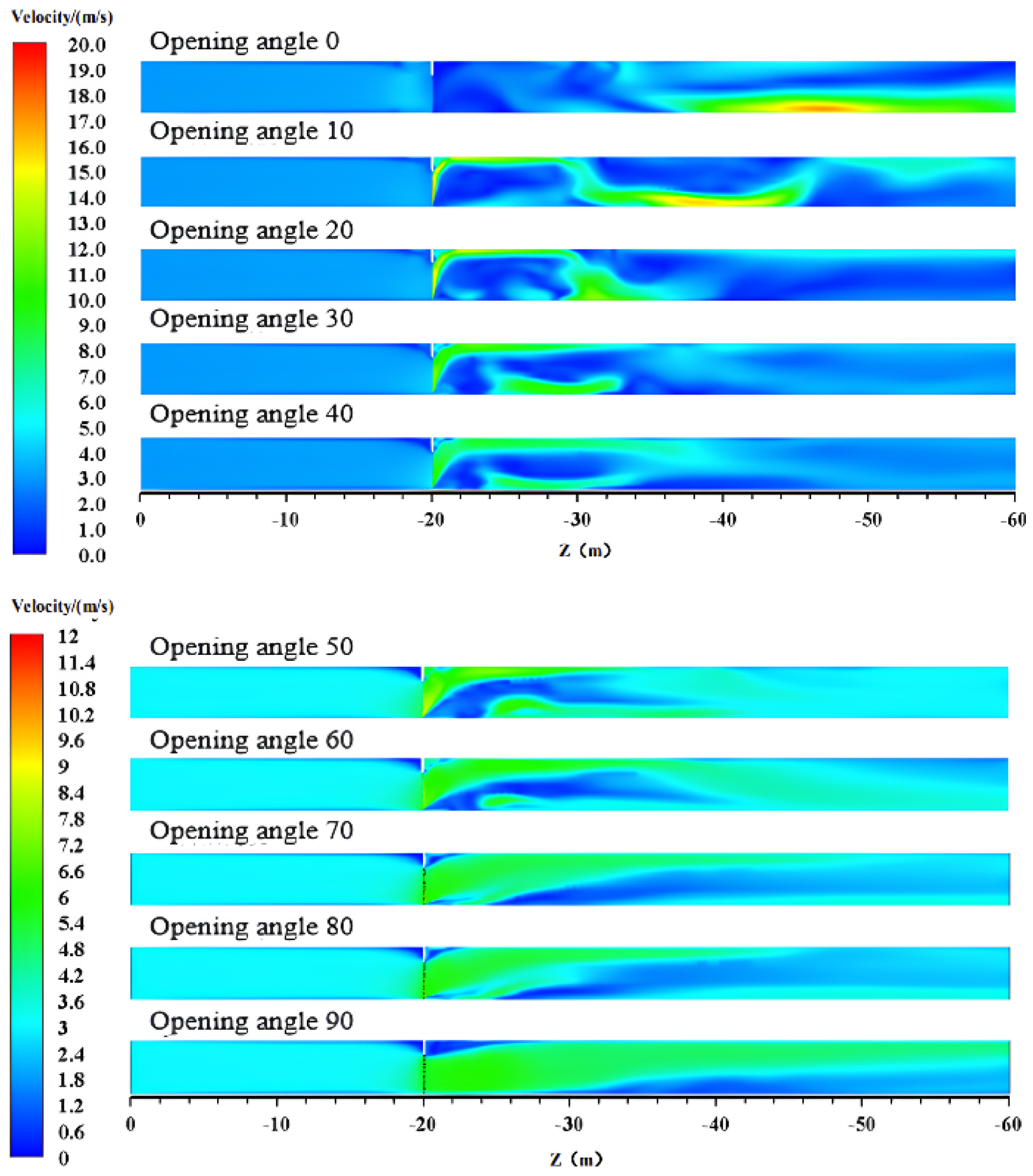
According to the opening angle of the wind window in the longitudinal section of the wind speed distribution, at different adjustment angles of the wind window, the wind flows uniformly through the window. After the rapid change in the flow field, the blades of the window guide the windshield effect of the window, such that the airflow to the upper side of the roadway is folded. Conversely, the smaller the opening angle of the window, the greater the change in velocity [7,8,9].

In the Figure 3 to ensure the reliability and numerical accuracy of the simulation results, a mesh independence study was conducted. Three mesh densities were generated for the same computational domain and boundary conditions: coarse, medium, and fine. The total number of cells for the coarse, medium, and fine meshes was approximately 0.6 million, 1.2 million, and 2.4 million, respectively. The airflow velocity and gas concentration at a monitoring section downstream of the louver damper, along with the pressure drop across the damper, were selected as the evaluation parameters. The comparison results showed that as the mesh density increased from medium to fine, the variation in airflow velocity and pressure drop was less than 1.5%, indicating that further mesh refinement had a negligible effect on the simulation results. Considering both computational efficiency and numerical accuracy, the medium mesh with approximately 1.2 million cells was selected for all subsequent simulations.

CFD Model and Numerical Setup: The airflow in the return airway with a remotely adjustable louver damper was simulated using computational fluid dynamics (CFD). Air was treated as an incompressible Newtonian fluid, and the flow was assumed to be turbulent due to the relatively high Reynolds number in the ventilation roadway.

The governing equations consisted of the continuity equation and the three-dimensional Reynolds-averaged Navier–Stokes (RANS) equations. Turbulence effects were modeled using the Realizable k–ε turbulence model, which has been widely applied in mine ventilation simulations and has demonstrated good performance in predicting airflow separation and recirculation in confined spaces.

Boundary Conditions:

Inlet boundary: A velocity inlet boundary condition was applied at the upstream section of the airway. The inlet air velocity was set to 3.0 m/s, corresponding to the actual ventilation conditions of the working face.

Outlet boundary: A pressure outlet boundary condition was imposed at the downstream section, with the gauge pressure set to 0 Pa.

Wall boundary: All airway walls, louver blades, and damper surfaces were treated as no-slip walls. Standard wall functions were employed for near-wall treatment.

Modeling Assumptions: To reduce computational cost while maintaining sufficient accuracy, the following assumptions were adopted. The airflow was assumed to be steady-state. Thermal effects were neglected, and the flow was considered isothermal. The influence of dust particles on the airflow field was ignored, and only the gas phase was simulated. The deformation of the louver damper was neglected, and all solid structures were assumed to be rigid.

Numerical Schemes and Solver Settings: The numerical simulations were performed using a pressure-based steady-state solver. The pressure–velocity coupling was handled using the SIMPLE algorithm. Second-order upwind discretization schemes were applied to the momentum equations and to the turbulent kinetic energy and dissipation rate equations to ensure sufficient numerical accuracy.

The convergence of the solution was monitored using both residuals and key physical variables. The residuals of the continuity, momentum, turbulent kinetic energy, and turbulent dissipation rate equations were required to be less than 1 × 10⁻⁵. In addition, the airflow velocity and pressure at selected monitoring points downstream of the louver damper were tracked during the iteration process. The solution was considered converged when these monitored variables became stable and showed no further noticeable variation.

Each simulation case required approximately 1500–2500 iterations to achieve convergence.

2.1.2. Calculation of the Equivalent Wind Resistance of the Windscreen

A change in the angle of inclination of the wind window, on the one hand, changes the cross-sectional area of the flow, on the other hand, causes a change in the direction of flow, leads to rapid changes in the distribution of flow velocity, which leads to the formation of friction, collision of fluids within the local area, and the formation of local resistance. Because wind network solution software often uses the same wind resistance for wind doors, wind windows, and other ventilation structures.

When using the ventilation network solution system to optimize the wind network and perform equivalent calculations, the resulting scheme should also adjust the branch wind resistance as an additional branch wind resistance. Therefore, the local wind window resistance in this work is expressed in terms of equivalent wind resistance R.

Wind pressure and air volume sensors are installed at a stable location in the wind flow upstream and after the local resistance adjustment object. The incoming side of the wind flow is given as the measurement point i, and the outgoing side is given as the measurement point j. According to the Bernoulli equation, the following is established:

$$h_{i-j}=(p_i-p_j)+(z_i-z_j){\rho }_{ij}g+{\displaystyle \frac{({\rho }_i{v}_i^2-{\rho }_j{v}_j^2)}{2}}$$

(1)

where $h_{i-j}$ is the ventilation resistance between the two measuring points, Pa; $p_i,p_j$ is the static pressure measurement value at two measuring points, Pa; $z_i,z_j$ is the height above sea level at two points of measurement, m; ${\rho }_i,{\rho }_j$ is the density of humid air at two measurement points, kg/m³; ρ_ij is the average value of air density between two measuring points, kg/m³; v_i, v_j is the air velocity at two measurement points, m/s.

$$R=y_0+A_1{e}^{-a/t_1}+A_2{e}^{-a/t_2}$$

(2)

In Equation (2), R represents equivalent wind resistance (Pa·s/m³), y₀, A₁, A₂ are fitting constants, a is the window opening angle ( ), and t₁, t₂ are time constants (s). This empirical formula was derived from experimental data to characterize the nonlinear relationship between wind resistance and window angle.

2.1.3. Mathematical Modeling and Identification of the Windscreen Ventilation System

After completing the construction of the automatic windshield control system, a mathematical model of the control object is needed for the control algorithm. This can be obtained by identifying the system in automatic windshield control for wind regulation [10,11,12].

In this paper, the method of least squares was chosen to identify the parameters. Let the input be u(t), and the output be x(t), and the general expression of the parametric model is as follows:

$$x\left(t\right)+a_{1}x(t-1)+\cdots +a_{n}x(t-n)=b_{0}u\left(t\right)+\cdots +b_{n}u(t-n)$$

(3)

$$y(t)=x(t)+w(t)$$

(4)

Let y(t) be the observed value of x(t) and $w\left(t\right)$ the random perturbation. Assuming that 3 is white noise with a mean of 0, the following is established:

$$\xi (t)=w(t)+\sum _{i=1}^n{a}_{i}w(t-i)$$

(5)

After binding, the following is established:

$$y\left(t\right)=-a_{1}y(t-1)-\cdots -a_{n}y(t-n)+b_{0}u\left(t\right)+\cdots +b_{n}u(t-n)+\xi \left(t\right)$$

(6)

$\xi \left(t\right)$ Indicates measurement error due to input and output values and internal system noise. By measuring m + N inputs and outputs, N equations can be obtained as follows:

$$\left\{\begin{array}{l}y(m+1)=-a_{1}y\left(m\right)-\cdots -a_{m}y\left(1\right)+b_{0}u(m+1)+\cdots +b_{n}u\left(1\right)+\xi (m+1)\\ y(m+2)=-a_{1}y(m+1)-\cdots -a_{m}y\left(2\right)+b_{0}u(m+2)+\cdots +b_{n}u\left(2\right)+\xi (m+2)\\ \cdots \\ y(m+N)=-a_{1}y\left(m\right)-\cdots -a_{m}y\left(N\right)+b_{0}u(m+N)+\cdots +b_{n}u\left(N\right)+\xi (m+N)\end{array}\right.$$

(7)

$$y=\left[\begin{array}{l}y(m+1)\\ y(m+2)\\ ⋮\\ y(m+N)\end{array}\right],\theta =\left[\begin{array}{l}{a}_1\\ ⋮\\ a_m\\ b_0\\ ⋮\\ b_m\end{array}\right],\xi =\left[\begin{array}{l}\xi (m+1)\\ \xi (m+2)\\ ⋮\\ \xi (m+N)\end{array}\right]$$

(8)

$$\omega =\left|\begin{array}{cccccc}-y\left(m\right)& \cdots & -y\left(1\right)& u(m+1)& \cdots & u\left(1\right)\\ -y(m+1)& \cdots & -y\left(2\right)& u(m+2)& \cdots & u\left(2\right)\\ ⋮& \cdots & ⋮& ⋮& \cdots & ⋮\\ -y(m+N)& \cdots & -y\left(N\right)& u(m+N)& \cdots & u\left(N\right)\end{array}\right|$$

(9)

$$y=\omega \theta +\xi$$

(10)

Let the remainder $e$ be the difference between $y$ and $\stackrel{\wedge }{y}$, the following is established:

$$\stackrel{\wedge }{y}=\omega \stackrel{\wedge }{\theta }$$

(11)

$$e=y-\stackrel{\wedge }{y}=y-\omega \stackrel{\wedge }{\theta }$$

(12)

In the method of least squares, the minimum sum of the squares of the residuals is usually taken as the optimal estimate. Let us assume that L observations are made, and the performance indicators are as follows:

$$J={\sum }_{k=1}^L{e}^2={\sum }_{k=1}^L{\left[y-\omega \stackrel{\wedge }{\theta }\right]}^2=(y-\omega \stackrel{\wedge }{\theta }{)}^T(y-\omega \stackrel{\wedge }{\theta })$$

(13)

Solve the issue of displacement as follows:

$${\displaystyle \frac{\delta J}{\delta \stackrel{\wedge }{\theta }}}=2{\omega }^{T}y+2{\omega }^T\omega \stackrel{\wedge }{\theta }=0$$

(14)

You can obtain the best estimate as follows:

$$\stackrel{\wedge }{\theta }={({\omega }^T\omega )}^{-1}{\omega }^{T}y$$

(15)

This time, we use MATLAB R2024b System Identification Toolbox (SIT) to identify the wind window control system model. This mainly uses the structural model of least squares for systematic identification and provides functions such as loading and preprocessing input/output data, selecting and establishing the type of model structure, evaluating model parameters, and validating the model in graphical interactive mode, in addition to model validation and other functions [13,14,15].

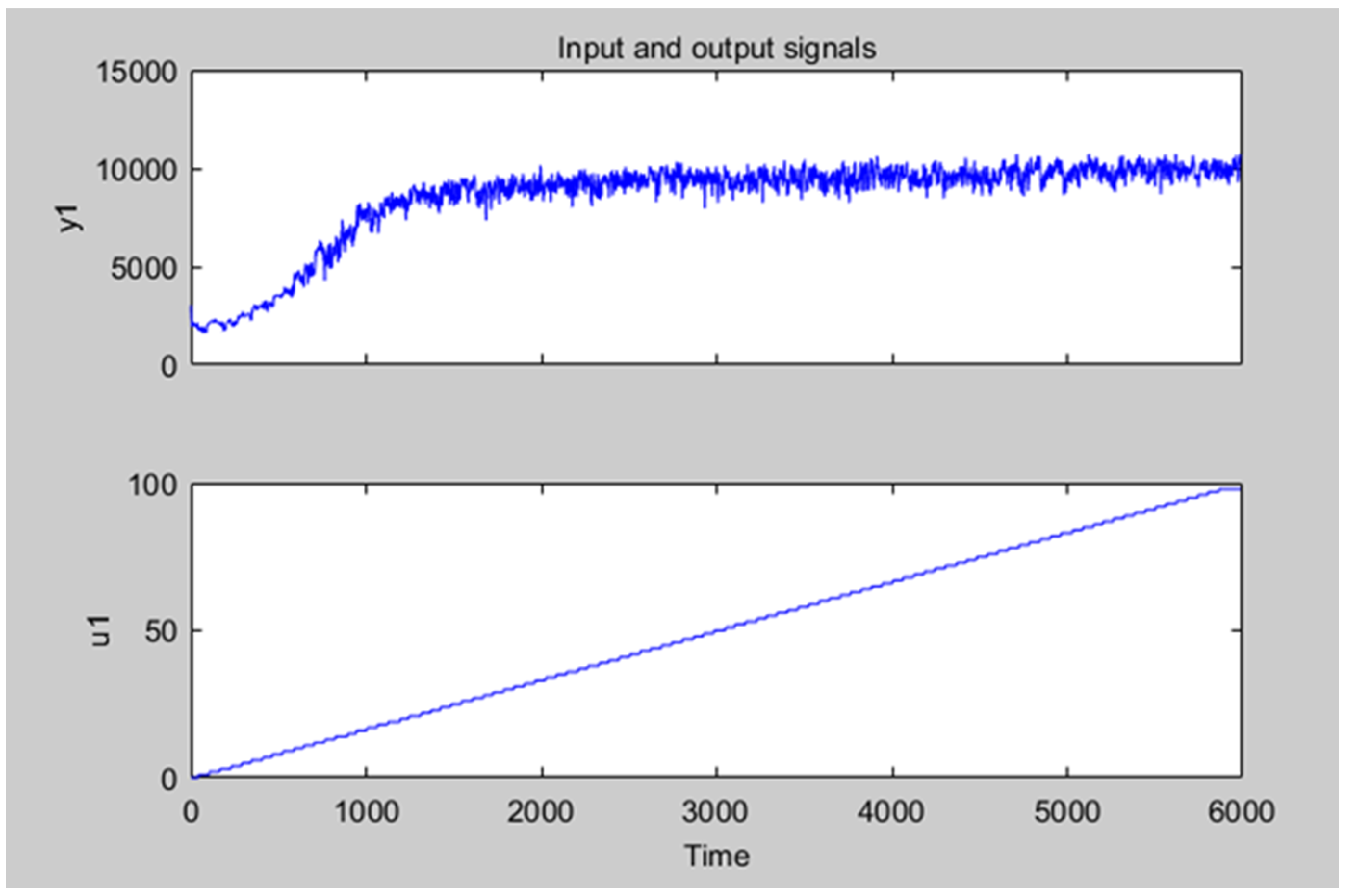
The curve of the dependence of input and output data is shown in Figure 4.

Figure 5 presents raw time-series data of input signals (e.g., ventilation window control commands) and their corresponding output responses (e.g., airflow velocity or air pressure in the roadway), which are used for system identification. This figure reflects the dynamic characteristics of the controlled object. It serves as the data foundation for subsequently deriving the transfer function model of the ventilation window control system (i.e., Equation (16)) using the least-squares method and the MATLAB System Identification Toolbox. The dynamic response relationship between the input and output curves in the figure provides key and reliable real-world data support for establishing a high-precision mathematical model. Further, it enables the training of the DQN-based intelligent ventilation decision-making algorithm.

Equation (16) is a data-driven, second-order transfer function model with a zero, obtained through system identification. Its coefficients are derived from the optimal mathematical fitting of experimental/simulation data of the windshield control system, accurately characterizing the system’s dynamic behavior. This model constitutes the core computational environment for the subsequent training and testing of deep reinforcement-learning intelligent algorithms. A transfer function model is used to identify the model; the number of poles is set to 2, and the zero point is set to 1. The final model of the windshield control system obtained using the identification toolkit is 82.53% consistent with the actual data.

$$G(s)={\displaystyle \frac{7.174s+0.0003817}{s^2+0.007983s+0.00002727}}$$

(16)

2.2. Reinforcement Deep Learning in Smart Ventilation System Design

2.2.1. Basics of Reinforcement Learning

Reinforcement learning is a dynamic process in which model parameters, such as strategies and value functions, are updated through continuous interaction with the environment. In the process of mine ventilation control, due to the complexity of the tunnel environment, it is difficult to investigate the implicit relationship between the ventilation system outlet control parameters and the concentration of gas and dust, oxygen, and carbon dioxide in the tunnel. Therefore, it is difficult to obtain a general control strategy based on experience [16,17,18].

In continuous coal mining, the concentrations of gas dust, oxygen, and carbon dioxide in the roadway change, and the wind turbine control strategy must be adjusted accordingly. Reinforcement learning enables you to develop an optimal management strategy for each operational period in real time, adapting to changes in the tunnel environment.

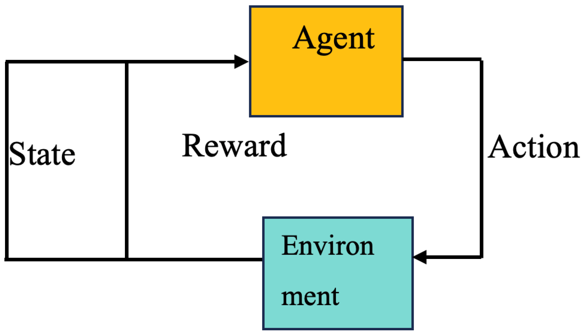
In Figure 6 the goal of reinforcement learning is to maximize total reward through policy optimization, which coincides with the goal of Markov decision-making processes, which is why reinforcement learning is often modeled as a Markov decision-making process [19,20,21].

The Markov decision-making process can be represented as a five <$S,A,P,R,\gamma$>, where $S$ is a set of states, $A$ is a finite set of actions, and $P$ is a matrix of probabilities of the transition of states. The reward function $R$ is an expectation, representing the reward for achieving a state, and $\gamma$ is the discount factor.

2.2.2. Deep Reinforcement Mine Ventilation Intelligent Decision-Making System Training Scheme

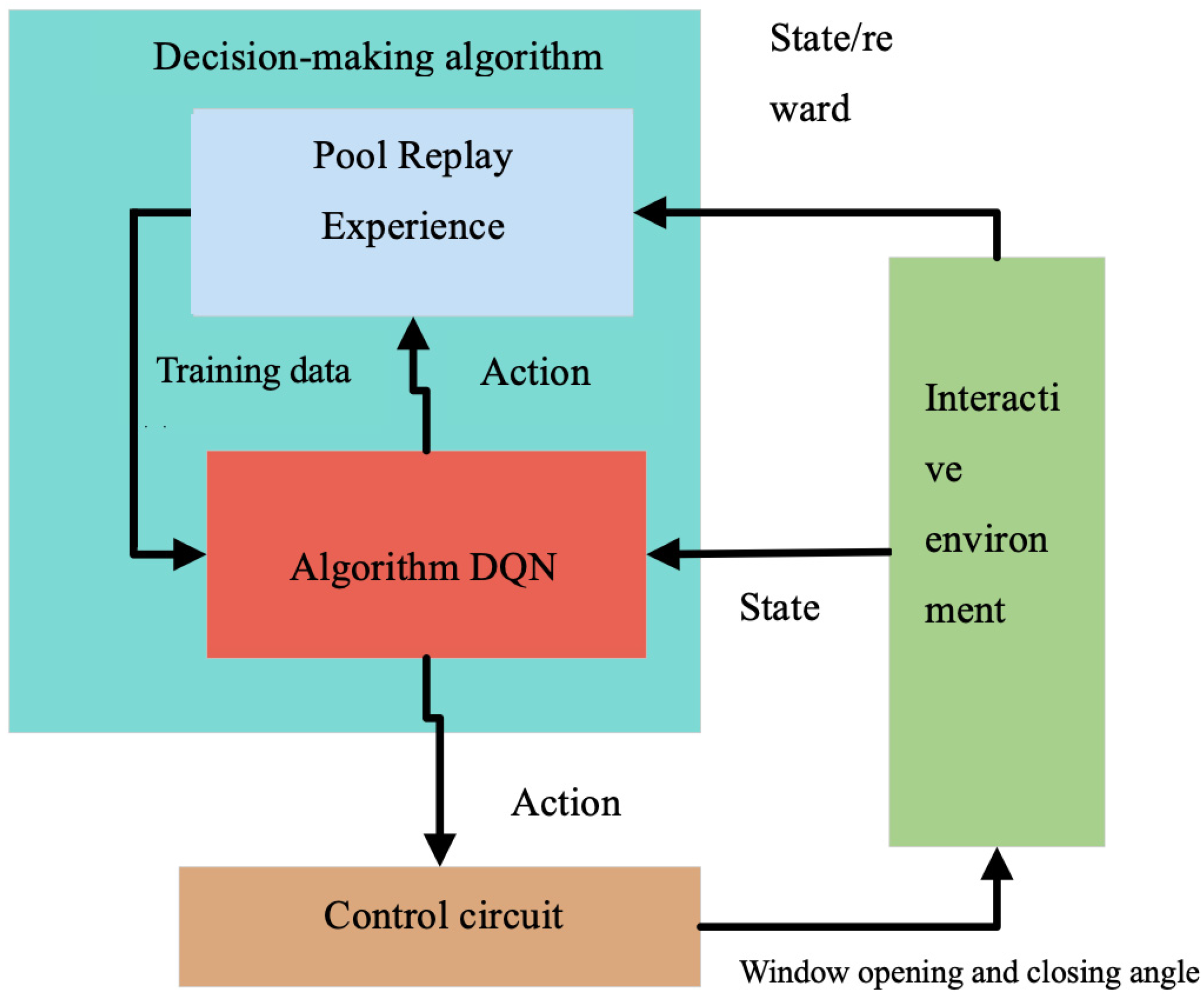
The intelligent mine ventilation system makes decisions based on the environmental information obtained by the sensor system, mainly including gas concentration, dust concentration, oxygen concentration, carbon dioxide concentration and other data, to ensure a safe and reasonable regulation scheme for the opening and closing angle of the ventilation window, to change the distribution of airflow in the tunnel, and its performance is an important indicator of the system’s ability ventilation [22,23,24]. In this work, deep reinforcement learning is used as the decision-making method for the intelligent mine ventilation system, and its training scheme is shown in Figure 7.

The DQN algorithm is chosen as the decision-making algorithm for intelligent mine ventilation in this paper, which uses data from interactions between the mine ventilation system and the road environment to train and optimize the management strategy of the intelligent mine ventilation system.

2.3. Modeling the Mine Ventilation System and Building a Reinforcement-Learning Environment

In studies [25,26,27], first, a BP neural network model for mine ventilation is created after analyzing various influencing factors in the tunnel, then data samples are collected through experiments to complete the training of the mine ventilation environment model, such that it can realistically simulate the behavior and operation of the ventilation system. Finally, based on this model, a reinforcement-learning environment for mine ventilation is created using the Gym architecture. In the network, the main parameters are as follows: learning rate α = 0.0003, discount factor γ = 0.99, exploration rate ε_initial = 1.0, ε_final = 0.05, ε_decay = linear decay over 100,000 steps, and replay buffer size = 1,000,000.

2.3.1. How VR Neural Networks Work

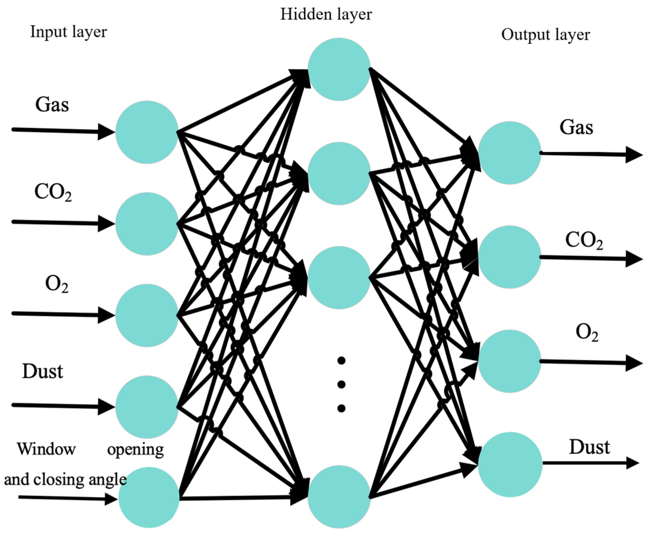
BP Neural Network is the most representative algorithm in the field of artificial intelligence due to its relatively simple topology, strong nonlinear mapping capability, strong generalization ability, high accuracy, and certain fault tolerance. The BP Neural Network consists of an input layer, an intermediate layer, and an output layer, with neurons in adjacent layers connected and those within the same layer unconnected [28,29,30]. The neurons in the two adjacent layers are connected, while those in the same layer are not; the influence of the adjacent neurons is reflected in their respective weights. The schematic diagram is shown below in Figure 8:

To do this, first select the appropriate activation function. Then, initialize the weights and thresholds between the input and implied layers, as well as between the implied and output layers. After that, the output value of the implied layer is calculated using the following formula:

$$H_i=f\left[{\sum }_{i=1}^n{x}_i{\omega }_{ij}+a_i\right],j=\mathrm{1,2},\cdots ,m$$

(17)

where $H_i$ is the output value of the implicit layer, $f$ is the transfer function, $x_i$ is the input vector, and $m$ is the number of nodes in the implicit layer. ${\omega }_{ij},a_i$ are the weights and thresholds between the input and implicit layers, respectively.

Next, calculate the output value of the output layer as follows:

$$Q_k=f\left[{\sum }_{j=1}^r{H}_j{\omega }_{jk}+b_k\right],k=\mathrm{1,2},\cdots ,l$$

(18)

where $Q_k$ is the output value of the output layer, $l$ is the number of nodes in the output layer, and ${\omega }_{jk},b_k$ are the weights and thresholds between the implicit and output layers, respectively.

After that, the predicted value and the error between it and the actual value are calculated, $e$, as follows:

$$e=E(\theta )={\displaystyle \frac{1}{m}}{\sum }_{i=1}^k(y_k-o_k{)}^2$$

(19)

The resulting error, e, is then plugged into the next equation to adjust the bond weights, with $\eta$ being the learning rate.

$${\omega }_{jk}={\omega }_{jk}+\eta H_i{e}_k$$

(20)

$${\omega }_{ij}={\omega }_{ij}+\eta H_j(1-H_j)x_i{\sum }_{k=1}^m{\omega }_{jk}{e}_k$$

(21)

In this work, based on the mine’s ventilation system, the inlet layer consists of five parameters: gas concentration, dust concentration, oxygen concentration, carbon dioxide concentration, and the angle of opening and closing of the ventilation window. The hidden layer has 12 nodes according to the empirical formula, and the output layer consists of four parameters: gas concentration, dust concentration, oxygen concentration, and carbon dioxide concentration.

The input layer includes five parameters: gas concentration, dust concentration, oxygen concentration, carbon dioxide concentration, and the window opening angle. The output layer predicts the adjusted concentrations of the four gases. Airflow is indirectly represented by the window angle, as it directly influences ventilation volume. Sensors are located 10 m downstream of the window in a stable flow region.

2.3.2. Collect Trial Data and Verify Model Accuracy

The dataset was collected from the return airway of a coal mine in Ordos, Inner Mongolia. The roadway has a semi-circular arch section with a cross-sectional area of approximately 12.25 m² and maintains a steady airflow between 1.2 and 1.8 m/s. The dataset includes six variables: gas concentration (%), dust concentration (mg/m³), oxygen concentration (%), carbon dioxide concentration (%), airflow velocity (m/s), and the window opening angle (degrees). Data were recorded at a time resolution of 1 s. Sensors were installed 10 m downstream of the ventilation window in a stable flow region to minimize turbulence effects. The raw data contained occasional outliers due to sensor noise, which were removed using a sliding window median filter. Subsequently, all variables were normalized using Z-score normalization to facilitate model training. The total number of samples is 3630, and their components are presented in

Table 2. Partial sample of the dataset content.

Serial Number	Source Data				Window Opening and Closing Angle	Post-Modulation Data
	Gas Concentration (%)	Dust Concentration	Oxygen Concentration (%)	Carbon Dioxide Concentration (%)		Gas Concentration (%)	Dust Concentration	Oxygen Concentration (%)	Carbon Dioxide Concentration (%)
1	0.72	532	21.443	0.452	34	0.74	486	21.445	0.444
2	0.79	565	21.440	0.422	56	0.72	359	21.448	0.408
3	0.77	517	21.444	0.402	31	0.65	408	21.449	0.389
4	0.76	488	21.448	0.415	24	0.59	507	21.451	0.405
5	0.88	577	21.451	0.429	45	0.71	426	21.461	0.421
6	0.85	562	21.447	0.441	34	0.73	369	21.447	0.434
7	0.74	528	21.452	0.442	24	0.64	451	21.452	0.432
8	0.63	365	21.442	0.439	37	0.67	406	21.443	0.421
9	0.78	558	21.447	0.432	79	0.54	427	21.442	0.417
10	0.79	446	21.445	0.431	22	0.74	289	21.451	0.419
…	…	…	…	…	…	…	…	…	…
3623	0.71	493	21.441	0.435	34	0.73	524	21.459	0.414
3624	0.75	535	21.442	0.482	65	0.59	529	21.454	0.467
3625	0.83	552	21.437	0.421	74	0.62	518	21.427	0.401

.

The model training configuration is shown in

Table 3. Model hyperparameter configuration.

Hyperparameterization	Selected Values
Hidden layer activation function	RELU
Output Layer Activation Function	Tanh
Learning Speed	0.001
Optimization algorithm	Adam’s algorithm
Loss Function	MSE
Training Accuracy	0.001
Maximum number of training iterations	800

:

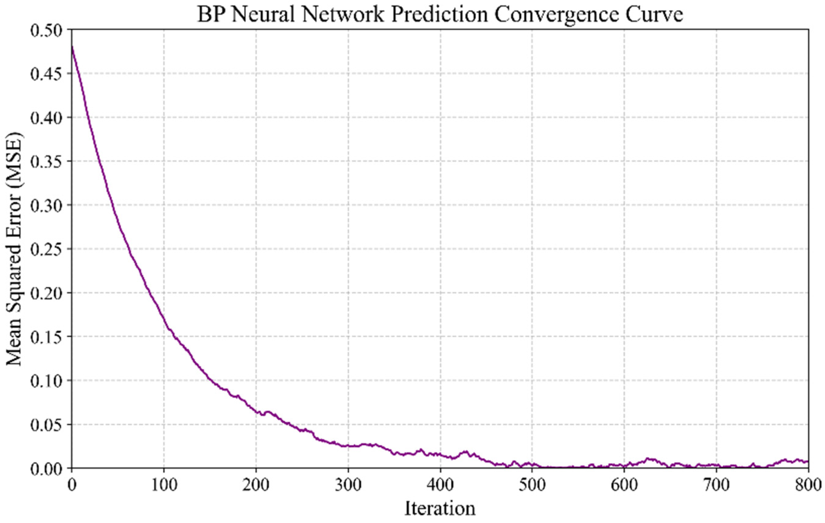
To ensure the accuracy of a prediction model based on a VR neural network, sample data is usually divided into two categories: training and test. In this paper, we select the first 3000 datasets for training the VR neural network, and the remaining 630 datasets are used as test samples to evaluate the network’s predictive and generalization abilities after training. The convergence curve of the prediction model based on the VR neural network is shown in Figure 9.

The horizontal axis shows the number of iterations, and the vertical axis shows the loss function value. It can be seen that at the initial stage, the loss function is large and fluctuates widely, but as the model is trained and optimized, the fluctuations gradually decrease as the loss function decreases and finally converge to a relatively stable level. After 525 iterations, the network’s average quadratic error converges to 0.0007 and remains stable. A model after 525 iterations can be used as a prediction model, and the updated parameters are preserved. To quantitatively evaluate the BP neural network’s predictive accuracy, we calculated the root mean square error (RMSE), mean absolute error (MAE), and coefficient of determination (R²) between the predicted and actual values on the test set. The results are as follows: RMSE = 0.023, MAE = 0.015, R² = 0.94. These metrics indicate that the model has high predictive accuracy and strong generalization.

2.3.3. Creating an Improved Learning Environment

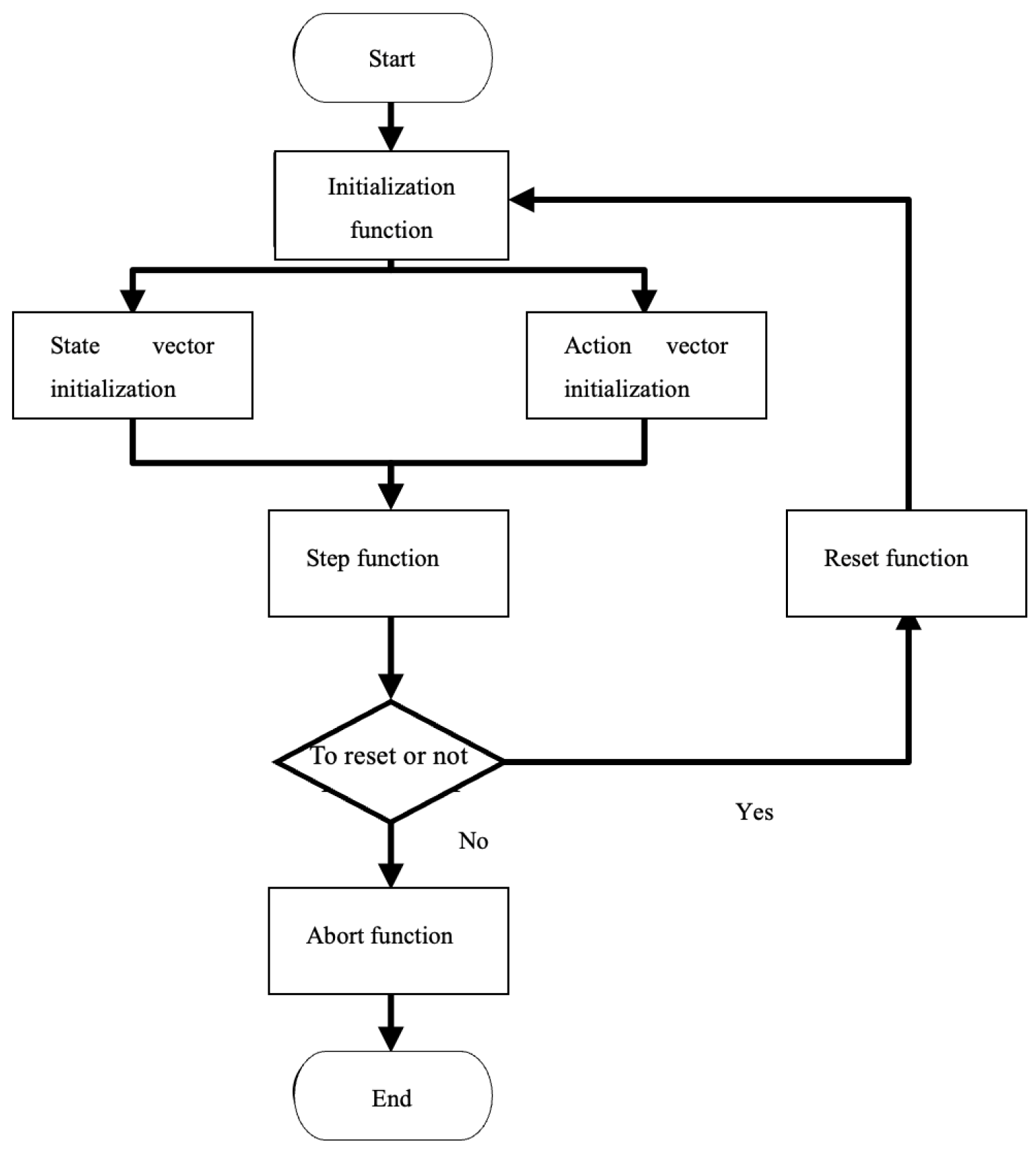
By combining the Gym architecture with the neural network model for mine ventilation VR [31,32,33], a reinforcement-learning environment for an intelligent mine ventilation control system was created. The full architecture of the Gym program is shown in Figure 10.

The initialization function sets the reinforcement-learning environment’s initial state and returns it. This includes defining the simulation time step and initial strategy for the mine ventilation control system.

The step function executes a given action in the current environment and observes the result. It receives a parameter that represents the action to be taken; performs an action in the current environment and observes its impact on the state of the environment and the reward signal; And finally, it returns three parameters: a new state, a reward signal, and a Boolean variable that shows whether the task is completed or not.

2.4. DQN-Based Decision-Making Algorithm for Intelligent Mine Ventilation

2.4.1. How the DQN Algorithm Works

The DQN algorithm was selected for this study over other reinforcement-learning methods (e.g., Policy Gradient, PPO) for several reasons. First, the control action (louver opening angle) in our problem is discrete (0–90 degrees), which aligns perfectly with DQN’s design for discrete action spaces. Second, the state space (multidimensional gas and dust concentrations) is high-dimensional and continuous. DQN’s use of a deep neural network as a function approximator is particularly effective in handling such complex state representations. Third, DQN’s mechanisms of experience replay and target network decoupling significantly improve training stability and sample efficiency, which is crucial for learning in a simulated environment with limited real-world interaction data.

Q-Learning is an autonomous reinforcement-learning algorithm that solves complex problems with discrete actions and states; it is based on the iterative process of value functions. The Q-Learning algorithm attempts to learn the value function of states and actions (the Q-function) by performing a greedy exploration of each activity in the state space. It uses a Q-table to store the expected reward of each action in each state, sets the initial Q-value to zero, and the intelligent body explores the environment by taking random actions. As the intelligent body receives rewards or penalties, the Q-values of the corresponding pairs of states and actions are updated, and the converging Q-values are eventually used to select the optimal action that maximizes the reward in the MDP task [34,35].

During training, the state-activity cost function is updated as shown in the following equation.

$$Q^{\pi }(s_t,a_t)=E\left[r\right(s_t,a_t)+\gamma Q^{\pi }(s_{t+1},\mu \left(s_{t+1}\right)\left)\right]$$

(22)

$$Q(s,a)=(1-{\lambda }_t)Q(s,a)+{\lambda }_t[r+\gamma {\mathit{max}}_{a\in A}Q(s\prime ,a\prime \left)\right]$$

(23)

The Q-Learning algorithm uses a table to store the function of the state value and the action, which is a disaster in terms of dimensionality when the number of states is large or even continuous. Meanwhile, the DQN algorithm uses a deep neural network to approximate the value function, a significant improvement over the Q-Learning algorithm for handling multidimensional data.

The loss function is also defined as follows:

$$Q(s,a)=(1-{\lambda }_t)Q(s,a)+{\lambda }_t[r+\gamma {\mathit{max}}_{a\in A}Q(s\prime ,a\prime \left)\right]$$

(24)

Using a gradient descent algorithm, the loss function is minimized, and the network parameters are updated iteratively until convergence.

2.4.2. Structure of the Decision-Making Algorithm for Intelligent Mine Shaft Ventilation Based on DQN

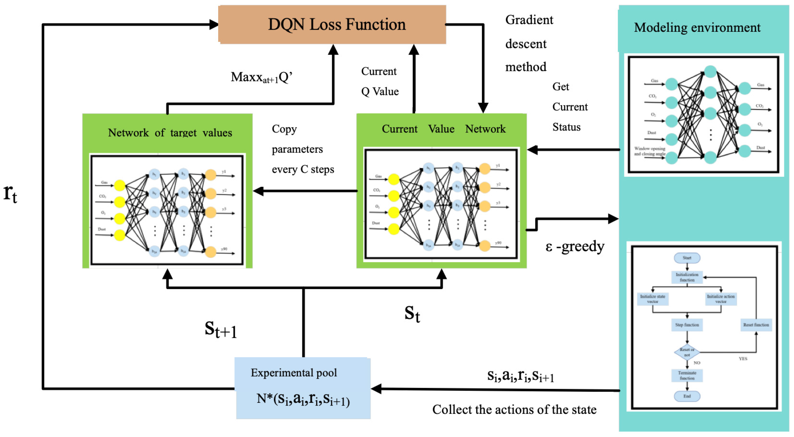
According to the DQN algorithm’s flow, the DQN-based intelligent mine ventilation decision-making algorithm is constructed as shown in Figure 10.

In the Figure 11, in the DQN algorithm for intelligent mine ventilation decision-making, the Q network and the target Q network interact with the simulation environment and are trained to learn an optimal smart mine ventilation strategy. During training, information about the current state of the mine environment is first entered into the Q network, which outputs the value of each action from the set of wind pipe control actions and selects the action $a_t$ according to the strategy $\epsilon -greedy$. After performing the action, it receives a reward $r_t$ according to the developed reward function and the new state of the roadway environment $s_{t+1}$. Then, the sequential data $(a_t,s_t,r_t,s_{t+1})$ is stored in the experience replay pool. Next, randomly selected empirical samples are entered into the Q network and the target Q network, and the DQN loss is calculated. The Q network is updated according to the loss function. Finally, the Q network parameters are synchronized with the target Q network every C time steps, and the cycle continues until the training is complete.

2.4.3. Simulation of Markov Decision-Making Processes for Intelligent Ventilation Systems in Mines

The state space, the action space, and the reward function are key factors that determine the effectiveness of reinforcement learning. In the intelligent mine ventilation system, the most basic action is the windshield opening and closing angle. The feedback information from the environment includes gas concentration, dust concentration, oxygen concentration, and carbon dioxide concentration in a predetermined position on the roadway. The condition, action, and reward will be determined according to this information.

In the state space of this work, gas concentration, dust concentration, oxygen concentration, and carbon dioxide concentration are taken as the system states. The data are measured by installing a set of sensors in the tunnel, wherein the gas sensor at time t is recorded as $C_t$, the oxygen concentration sensor at time t is recorded as $D_t$, the dust sensor at time t is written as $E_t$, and the carbon dioxide sensor at time t are written as $F$. Hence, the state space at time t is defined as follows: $S_t=(C_t,D_t,E_t,F_t)$.

Considering that the main action of the intelligent shaft ventilation system is only to control the opening and closing angle of the ventilation window, with a range of 0–90 degrees, there are 90 actions to choose from.

Reinforcement learning uses the agent’s body to interact with the state space to learn about rewards and punishments, choose actions to maximize reward, and develop a reasonable reward function.

$$R_t=\left\{\begin{array}{l}-100,c_d>1000\\ -500,c_g>1\\ -500,c_o<19.5,c_o>23.5\\ -200,c_c>5\\ {\mathit{log}}_{0.8}\left[{\displaystyle \frac{c_d}{100}}+c_g+c_o+c_c\right]\end{array}\right.$$

(25)

where $c_o$ is the concentration of oxygen, $c_c$ is the concentration of carbon dioxide, $c_g$ is the concentration of gas, and $c_d$ is the concentration of dust.

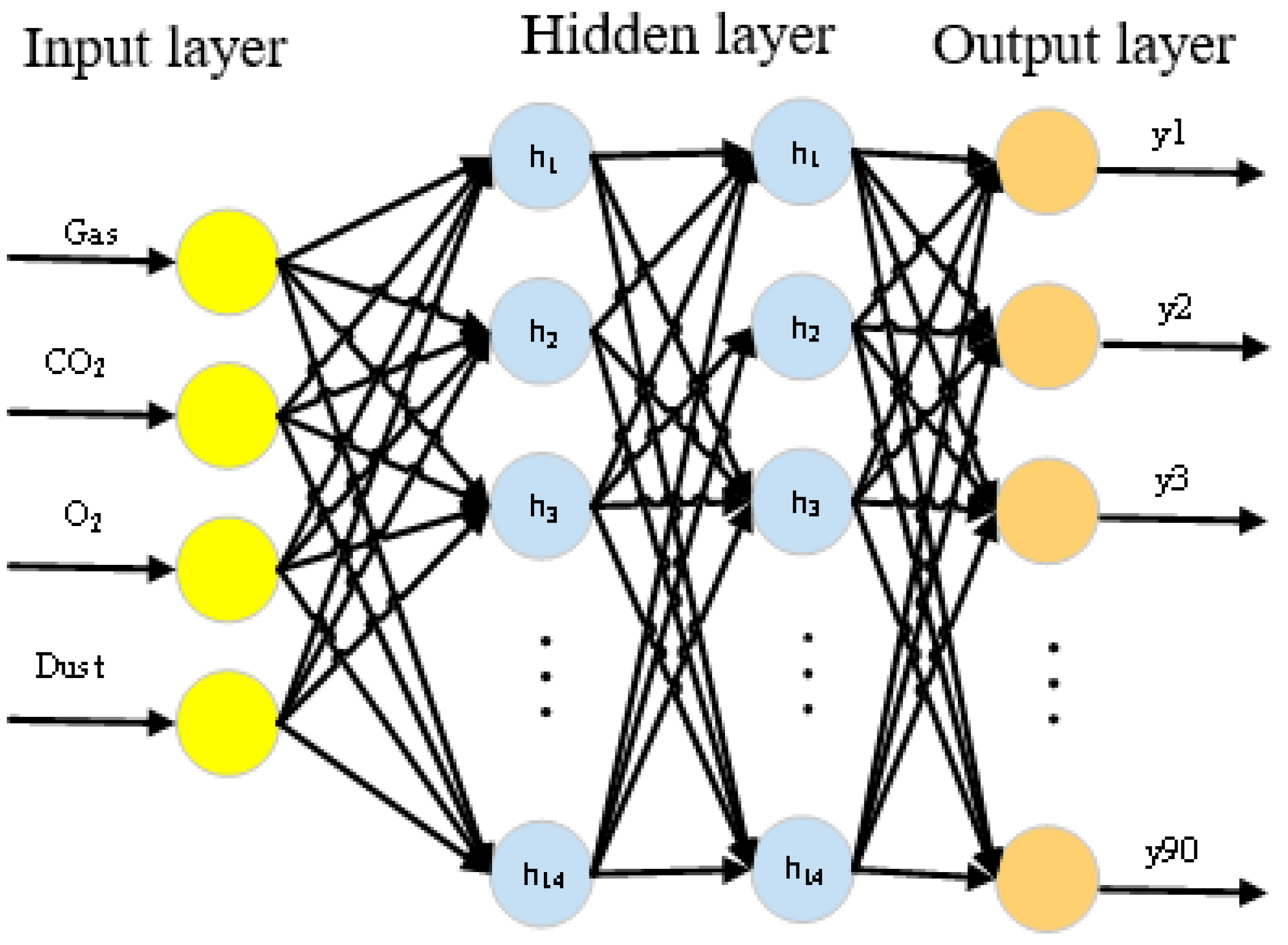
The topology of the Q-network consists of three layers: the input layer, the hidden layer, and the output layer. The input layer has as many neurons as the number of elements in the shaft ventilation state, which is four parameters. The number of neurons in the output layer equals the number of actions emitted by the intelligent controller; hence, the output layer has 90 nodes. There are also two hidden layers, each with 14 nodes, as shown in Figure 12. The Tanh function is used as the hidden-layer activation function, the ReLU function is used as the output-layer activation function, MSE is used as the loss function, and the Adam algorithm is used to update the neural network. The structure of the target Q-network and the Q-network is the same.

2.4.4. Validation of Simulation and Analysis of Results

The following hardware was used in this work: Windows 11 operating system, Intel Core i7-10700@3.80 GHz processor, 16 GB DDR3 1600 MHz memory, TensorFlow 2.1.8 deep-learning framework, and Python 3.7.0 programming language. When setting up the mine ventilation environment, we were guided by the OpenAI Labs Reinforcement-Learning Function Library (Gym), which provided standard environment specifications and functions.

The parameters of the DQN algorithm training process are shown in

Table 4. The parameters of the DQN algorithm training process.

Parameter	Numeric Value	Description
Experience Pool Size	3000	Maximum number of transition samples stored for training.
Batch Size	64	Number of samples randomly selected from the buffer for each training step.
Discount Rate	0.95	Discount rate for future rewards, ranging from 0 to 1.
$\epsilon -greedy$ Initial probability of the algorithm $\epsilon$	0.9	Initial probability of taking a random action in an ε-greedy policy.
Probability attenuation factor $\epsilon$	0.99	Minimum exploration rate after decay.
$\epsilon -greedy$ Final probability of the algorithm $\epsilon$	0.1	Multiplication factor for ε after each episode (linear decay).
Frequency of updating the parameters of the target network	50	Number of steps between copying the Q-network parameters to the target network.
Number of training rounds	600	Step size for the Adam optimizer.
Maximum number of steps	100	Total number of training episodes.

.

The size of the experiment visit buffer D is set to 3000 to ensure that the algorithm is trained on a sufficient number of samples; the batch size of the data samples selected for training is set to 64, which is suitable to accelerate the algorithm’s convergence; the cumulative return discount factor $\gamma$ is set to 0.95; the initial value $\epsilon$ used to learn the strategy is set to 0.9; the $\epsilon$ attenuation factor set to 0.99, which will be multiplied by the attenuation factor in each round $\epsilon$ until the minimum value is reached; the minimum value is $\epsilon$ set to 0.1; the refresh rate of the target Q network is set to 50, which means that the parameters of the Q network are copied to the target Q network every 50 steps. The decay ratio $\epsilon$ is set to 0.99, and $\epsilon$ multiplied by the decay factor in each round, until it reaches the minimum value; the minimum value is $\epsilon$ set to 0.1; the refresh rate of the target Q network is set to 50, that is, the parameters of the Q network are copied to the target Q network every 50 steps; the maximum number of steps of the T round is set to 100, and the total number of rounds of experiments is set to 600.

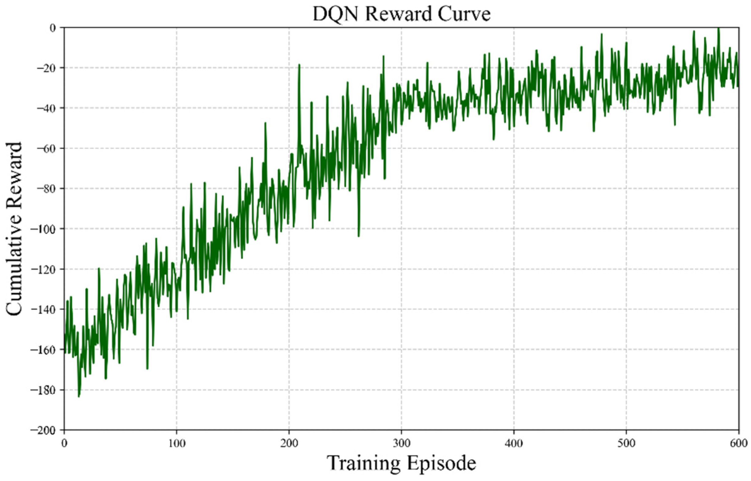
The total rewards received by the intelligences in each iteration are summed up. A reward convergence curve is plotted to visually observe whether the algorithm gradually improves decision-making and whether it reaches a steady state during the learning process. The DQN algorithm’s reward convergence curve is shown in Figure 13.

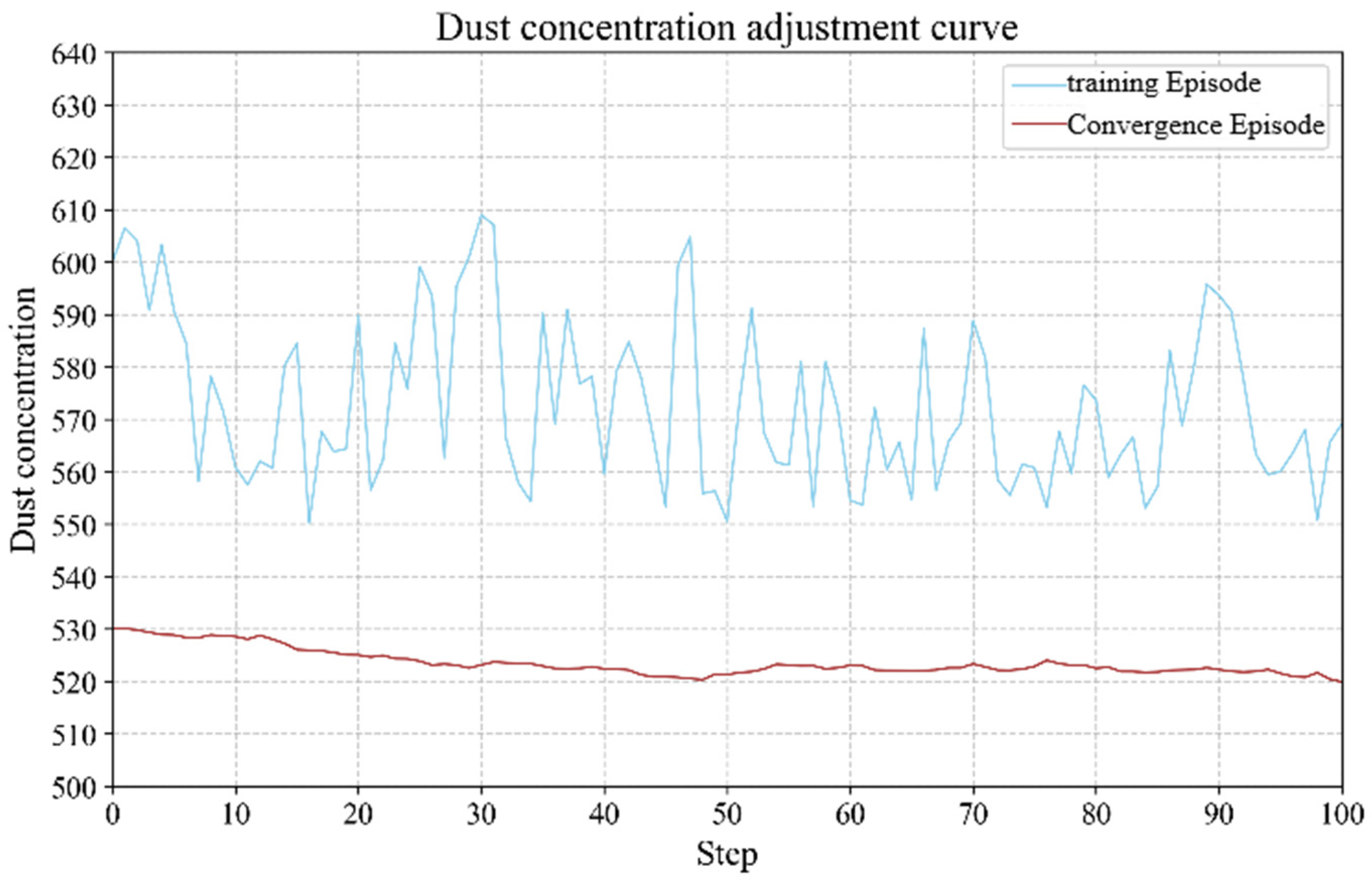
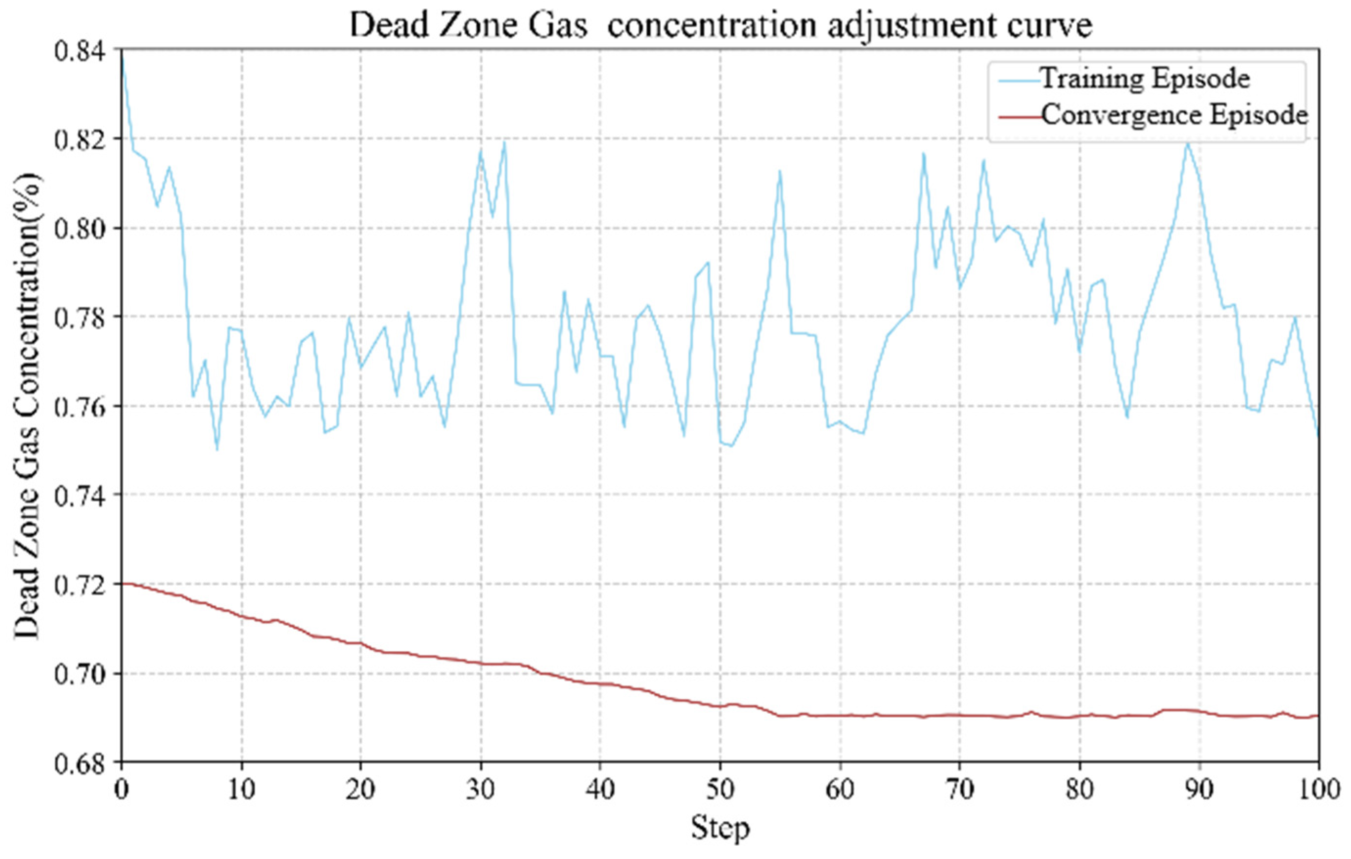
As can be seen from the figure, at the beginning of the algorithm execution, the cumulative reward is relatively small, because at the initial stage, the algorithm needs to explore the state space and action space, try different strategies to find the optimal solution, and the randomness of the choice of actions is very large. The neural network model learns to cope with random changes in the simulated mine environment, and the intellectual organ learns to adopt the appropriate strategy in response to changes in environmental parameters, thereby keeping the value of remuneration consistently high and increasingly stable. Dust concentration control curve is shown in Figure 14. Gas concentration control curve is shown in Figure 15. The reward value is always maintained at a high level and becomes increasingly stable.

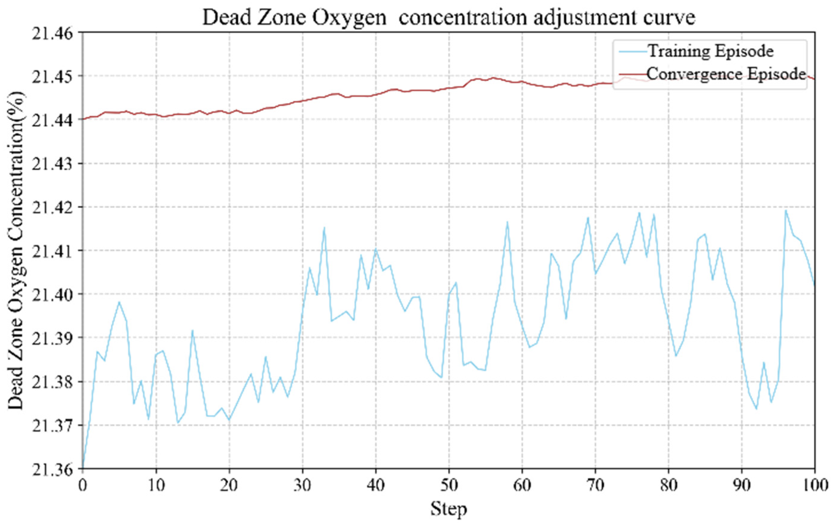
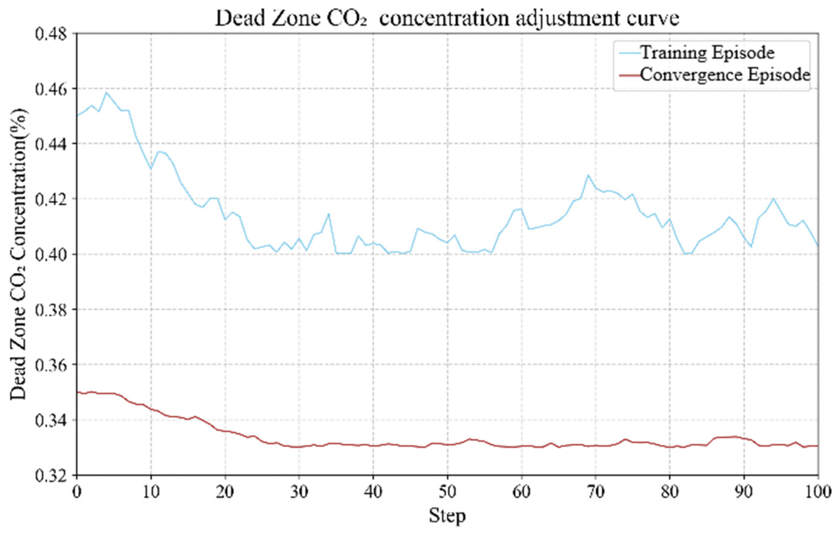
To visualize changes in the concentration ns of gas, dust, oxygen, and carbon dioxide in the tunnel during training of the DQN algorithm, the algorithm was set at the training stage and in one of the rounds after algorithm convergence, respectively. Gas concentration control curve is shown in Figure 16. Carbon dioxide concentration adjustment curve is shown in Figure 17.

To test the performance of the trained algorithm, five different initial gas and dust concentrations are used in this test, and the trained algorithm selects the optimal control action for each group of gas and dust concentrations based on the Q-value. Finally, the algorithm’s performance is evaluated by applying the appropriate control scheme. The optimal control actions for the different initial states and the corresponding post-control state values are given in

Table 5. Optimal control actions and post-control state values.

Serial Number	Source Data				Window Opening and Closing Angle	Post-Modulation Data
	Gas Concentration (%)	Dust Concentration	Oxygen Concentration (%)	Carbon Dioxide Concentration (%)		Gas Concentration (%)	Dust Concentration	Oxygen Concentration (%)	Carbon Dioxide Concentration (%)
1	0.78	587	21.443	0.433	54	0.66	486	21.445	0.444
2	0.72	465	21.442	0.422	51	0.65	387	21.449	0.408
3	0.74	517	21.448	0.402	41	0.68	429	21.444	0.389
4	0.78	543	21.441	0.429	62	0.59	411	21.462	0.402
5	0.88	573	21.455	0.412	49	0.73	422	21.467	0.408

.

While this study focuses on a single roadway, the proposed DQN-based control framework is scalable to mine-wide ventilation networks. Future research will integrate ventilation network simulation with multi-agent reinforcement learning to coordinate multiple windows and fans, achieving dynamic “on-demand air distribution” across the entire mine.

3. Conclusions

The DQN-based intelligent decision-making algorithm effectively optimized the ventilation control strategy in underground tunnels.

After applying the proposed control scheme, the concentrations of dust and harmful gases were significantly reduced.

The carbon dioxide concentration decreased, while the oxygen concentration increased, indicating an overall improvement in underground air quality.

The results demonstrate that the DQN algorithm can adaptively regulate ventilation parameters under dynamically changing underground environmental conditions.

The proposed DQN-based ventilation management strategy provides an effective solution for dynamic ventilation regulation, improving both safety and environmental stability in underground mines. It solves the problems of a scarcity of marking data and the difficulty of accurately modeling system dynamics.

References

1. Zhou, F.; Xin, H.; Wei, L.; Shi, G.; Xia, T. Research progress of mine intelligent ventilation theory and technology. Coal Sci. Technol. 2023, 51, 313–328. [Google Scholar] [CrossRef]
2. Xu, X.; Wang, K.; Zhang, Q.; Yao, Y. A Comprehensive Evaluation of Intelligent Coal Mine Ventilation Systems in the Internet of Things. Hum.-Centric Comput. Inf. Sci. 2023, 13, 46. [Google Scholar] [CrossRef]
3. Xu, X. Research on precise monitoring and hidden danger intelligent identification technology of ventilation network in Yuka No.1 mine. Int. J. Front. Eng. Technol. 2024, 6, 22–28. [Google Scholar] [CrossRef]
4. Zhang, J.; Bai, X.; Dong, X.; Zhang, Y.; Song, Z.; Wu, S. Structural field breeding and evolution and control technology of coal-rock dynamic disasters. Coal Sci. Technol. 2025, 53, 82–95. [Google Scholar] [CrossRef]
5. Grishin, E.L.; Nakaryakov, E.V.; Trushkova, N.A.; Sannikovich, A.N. Experience in implementation of dynamic mine venti-lation control. Gorn. Zhurnal. 2018, 8, 103–108. [Google Scholar] [CrossRef]
6. Li, G.; Kocsis, C.; Hardcastle, S. Sensitivity analysis on parameter changes in underground mine ventilation systems. J. Coal Sci. Eng. 2011, 17, 251–255. [Google Scholar] [CrossRef]
7. Li, B.-R.; Inoue, M.; Shen, S.-B. Mine Ventilation Network Optimization Based on Airflow Asymptotic Calculation Method. J. Min. Sci. 2018, 54, 99–110. [Google Scholar] [CrossRef]
8. Koteleva, N.I.; Korolev, N.A.; Zhukovskiy, Y.L. Identification of the technical condition of induction motor groups by the total energy flow. Energies 2021, 14, 6677. [Google Scholar] [CrossRef]
9. Liu, J.; Guo, X.; Deng, L.J.; Jiang, Q.; Gao, K.; Zhao, D. Resistance variant single fault source diagnosis of mine ventilation system based on air volume characteristics with resistance variation. J. China Coal Soc. 2018, 43, 143–149. [Google Scholar] [CrossRef]
10. Jiang, S.M. Theory and application of mine ventilation network sensitivity. Saf. Coal Mine 2011, 42, 96–99. [Google Scholar] [CrossRef]
11. Klyuev, R.V.; Morgoeva, A.D.; Gavrina, O.A.; Bosikov, I.I.; Morgoev, I.D. Forecasting planned electricity consumption for the united power system using machine learning. J. Min. Inst. 2023, 261, 392–402. [Google Scholar]
12. Jiang, S.; Pei, S.; Qie, R. MATLAB-based programming of mine ventilation network solution. Shaanxi Coal 2010, 29, 28–29. [Google Scholar] [CrossRef]
13. Zemenkova, M.Y.; Chizhevskaya, E.L.; Zemenkov, Y.D. Intelligent monitoring of the condition of hydrocarbon pipeline transport facilities using neural network technologies. J. Min. Inst. 2022, 258, 933–944. [Google Scholar] [CrossRef]
14. Gao, J.L.; Zhang, X.B. Analysis on the changing rule of airflow’s temperature and humidity in wet airflow. J. Saf. Sci. Technol. 2007, 17, 136–139. [Google Scholar] [CrossRef]
15. Gao, J.L.; Zhang, X.B. Treatment of water evaporation on airway surface in Calculation of strata rock heat. J. Saf. Sci. Technol. 2006, 16, 23–28. [Google Scholar] [CrossRef]
16. Zhukovskiy, Y.L.; Korolev, N.A.; Malkova, Y.M. Monitoring of grinding condition in drum mills based on resulting shaft torque. J. Min. Inst. 2022, 256, 686–700. [Google Scholar] [CrossRef]
17. Wang, D.; Zhou, F. Development of a WINDOWS-based mine ventilation network solution software. J. China Univ. Min. Technol. 2000, 29, 41–44. [Google Scholar] [CrossRef]
18. Lowndes, I.S.; Fogarty, T.; Yang, Z.Y. The application of genetic algorithms to optimise the performance of a mine ventilation network: The influence of coding method and population size. Soft Comput. 2005, 9, 493–506. [Google Scholar] [CrossRef]
19. Manap, M.; Nikolovski, S.; Skamyin, A.; Karim, R.; Sutikno, T.; Jopri, M.H. An analysis of voltage source inverter switches fault classification using short time fourier transform. Int. J. Power Electron. Drive Syst. 2021, 12, 2209–2220. [Google Scholar] [CrossRef]
20. Watson, C.; Marshall, J. Estimating underground mine ventilation friction factors from low density 3D data acquired by a moving LiDAR. Int. J. Min. Sci. Technol. 2018, 28, 657–662. [Google Scholar] [CrossRef]
21. Efimov, I.; Gabdulkhakov, R.R.; Rudko, V.A. Fine-tuned convolutional neural network as a tool for automatic microstructure analysis of petroleum and pitch cokes. Fuel 2024, 376, 132725. [Google Scholar] [CrossRef]
22. Wang, Z.; Ren, T.; Ma, L.; Zhang, J. Investigations of Ventilation Airflow Characteristics on a Longwall Face—A Computational Approach. Energies 2018, 11, 1564. [Google Scholar] [CrossRef]
23. Van Tung, L.; Long, P.T.; Van An, N.; Vasilev, B. Compare the Efficiency of the Active Filter and Active Rectifier to Reduce Harmonics and Compensate the Reactive Power in Frequency Controlled Electric Drive Systems. Int. Conf. Eng. Res. Appl. 2020, 178, 242–253. [Google Scholar] [CrossRef]
24. Xu, G.; Huang, J.; Nie, B.; Chalmers, D.; Yang, Z. Calibration of Mine Ventilation Network Models Using the Non-Linear Optimization Algorithm. Energies 2017, 11, 31. [Google Scholar] [CrossRef]
25. Jo, B.W.; Khan, R.M.A.; Javaid, O. Arduino-based intelligent gases monitoring and information sharing Internet-of-Things system for underground coal mines. J. Ambient. Intell. Smart Environ. 2019, 11, 183–194. [Google Scholar] [CrossRef]
26. Qin, Z.; Chen, S.; Xu, X.; Zhao, M. Research on Key Technologies and System Construction of Smart Mine. In Proceedings of the 2020 5th Asia-Pacific Conference on Intelligent Robot Systems (ACIRS), Singapore, 22–24 July 2020. [Google Scholar] [CrossRef]
27. Shklyarskiy, Y.E.; Lobko, K.K.; Kuznetsova, Y.N.; Vorobyov, M.S. Investigation of the Composite Motor Load in the Presence of Higher Harmonics in the Electrical Network. Energ. Proc. CIS High. Educ. Inst. Power Eng. Assoc. 2024, 67, 285–299. [Google Scholar] [CrossRef]
28. Sychev, Y.A.; Aladin, M.E.; Serikov, V.A. Aleksandrovich, Developing a hybrid filter structure and a control algorithm for hybrid power supply. Int. J. Power Electron. Drive Syst. 2022, 13, 1625–1634. [Google Scholar] [CrossRef]
29. Serikov, V.A.; Kostin, V.N.; Yu Sychev, A.; Samet, H. Evaluation method of power quality in mine supply systems with high-powered high-voltage variable frequency drives. Min. Informational Anal. Bull. 2024, 12, 162–177. [Google Scholar]
30. Li, Y.; Li, J.; Deng, C.; Liu, R.Z. Improved algorithm of air quantity calculating resistance based on diagonal subnetwork. J. China Coal Soc. 2019, 44, 1147–1153. [Google Scholar] [CrossRef]
31. Liu, J.; Jiang, Q.; Liu, L.; Wang, D.; Huang, D.; Deng, L.; Zhou, Q. Resistance variant fault diagnosis of mine ventilation system and position optimization of wind speed sensor. J. China Coal Soc. 2021, 46, 1907–1914. [Google Scholar] [CrossRef]
32. Zhang, Z.; Li, Y.; Li, J.; Zhang, J.; Li, B. Architecture and implementation of intelligent ventilation precise control system. J. China Coal Soc. 2022, 48, 1596–1605. [Google Scholar] [CrossRef]
33. Kozhubaev, Y.; Ovchinnikova, E.; Viacheslav, I.; Krotova, S. Incremental Machine Learning for Soft Pneumatic Actuators with Symmetrical Chambers. Symmetry 2023, 15, 1206. [Google Scholar] [CrossRef]
34. Li, W.; Liu, Y.; Zhang, L. Model and numerical solution method the failure of air volume and air flow components in the ventilation network during the period of external fire. Coal Sci. Technol. 2025, 53, 196–212. [Google Scholar] [CrossRef]
35. Zhang, D.; Wu, B.; Jia, J.; Zhao, L.; Li, Y. Construction and application of “Dual-drive” pre-warning system for coal mine water disaster based on microseismic data and model. Coal Sci. Technol. 2023, 51, 242–255. [Google Scholar] [CrossRef]
Figure 1. Physical view of the underground automatic ventilation window.
Symmetry 18 00311 g001
Figure 2. Automatic downhole windshield model.
Symmetry 18 00311 g002
Figure 3. Distribution of wind velocity in the longitudinal median section at different windshield opening angles.
Symmetry 18 00311 g003
Figure 4. Grid design structure.
Symmetry 18 00311 g004
Figure 5. Diagram of the I/O relationship of raw data.
Symmetry 18 00311 g005
Figure 6. Scheme of intensive training.
Symmetry 18 00311 g006
Figure 7. Diagram of the training structure of the intelligent decision-making system for mine ventilation.
Symmetry 18 00311 g007
Figure 8. BP neural network diagram.
Symmetry 18 00311 g008
Figure 9. BP neural network prediction convergence curve.
Symmetry 18 00311 g009
Figure 10. Architecture of the Gym.
Symmetry 18 00311 g010
Figure 11. General control diagram of an intelligent ventilation system.
Symmetry 18 00311 g011
Figure 12. Topology of network Q.
Symmetry 18 00311 g012
Figure 13. DQN remuneration curve.
Symmetry 18 00311 g013
Figure 14. Dust concentration control curve.
Symmetry 18 00311 g014
Figure 15. Gas concentration control curve.
Symmetry 18 00311 g015
Figure 16. Oxygen concentration adjustment curve.
Symmetry 18 00311 g016
Figure 17. Carbon dioxide concentration adjustment curve.
Symmetry 18 00311 g017