Multivariate Time-Series Forecasting of Youth Unemployment in Turkey: A Comparison of Deep Learning and Econometric Models

Abstract

Youth unemployment remains one of the most persistent and structurally sensitive challenges in emerging economies, particularly in environments characterized by macroeconomic volatility and frequent shocks. This study investigates the dynamics and forecasting performance of youth unemployment in Turkey by adopting a symmetry-based multivariate framework that explicitly contrasts equilibrium-oriented and asymmetric temporal behaviors. Using monthly data covering the period 2009–2024, youth unemployment is modeled jointly with key macroeconomic indicators, including economic growth, inflation, overall unemployment, labor force participation, migration, exchange rates, and consumer confidence. The empirical strategy integrates traditional econometric models and modern machine learning approaches under a unified and leakage-free evaluation protocol. Stationarity and long-run properties of the series are examined using unit root tests and the Bayer–Hanck cointegration approach, followed by long-run coefficient estimation via FMOLS and DOLS. Forecasting performance is then compared across VARIMA, Prophet, and deep learning models (RNN, LSTM, and GRU), including both vanilla and hyperparameter-tuned specifications. The results reveal a clear performance hierarchy. VARIMA models, particularly the VARIMA (p = 2, q = 0) specification, consistently outperform all alternatives by a wide margin, achieving exceptionally low forecast errors. This finding indicates that youth unemployment in Türkiye is predominantly governed by symmetric co-movements and long-run equilibrium relationships among macroeconomic variables. Prophet and GRU models capture short-term and regime-sensitive fluctuations more flexibly, reflecting asymmetric temporal responses, but at the cost of higher forecast dispersion. In contrast, RNN and LSTM models exhibit limited generalization capability and are prone to overfitting in the small-sample macroeconomic context. As a result, this study positions the estimation of youth unemployment as both an econometric challenge and a symmetry-based analytical problem, offering new methodological and conceptual insights consistent with a fresh perspective.

1. Introduction

Unemployment has long been recognized as one of the most persistent socio-economic challenges globally, particularly with the accelerating effects of globalization, technological transitions, and repeated episodes of macroeconomic instability. Although classical economic expectations suggest that unemployment should decline during periods of economic expansion, many countries continue to experience chronic and structurally embedded unemployment. Youth are disproportionately affected by this trend: according to the International Labor Organization (ILO), global youth unemployment rates remain nearly twice those of general unemployment, with severe implications for social cohesion, equitable opportunities, and long-term development trajectories [1].

In the literature, two major theoretical traditions have shaped the understanding of youth unemployment. The first derives from the traditional neoclassical framework, which attributes youth unemployment primarily to labor supply constraints and insufficient job creation for new entrants. The second, rooted in post-Keynesian thought, emphasizes employment instability and demand-side fluctuations as key determinants. Complementing these views, the Schumpeterian perspective highlights the role of structural transformations such as technological change, sectoral shifts, and skill mismatches in driving youth unemployment [2].

Empirical studies further categorize the determinants of youth unemployment under three broad headings: structural, cyclical, and demographic factors. Structural factors arise when young individuals lack the skills and competencies demanded by the labor market or when education systems fail to equip them with relevant qualifications. Cyclical factors emerge during economic downturns, where inexperienced young workers face intensified layoffs and reduced hiring prospects [3]. Demographic factors, such as high youth population ratios and elevated labor force participation, increase competition for limited job opportunities and contribute to higher unemployment levels among young cohorts [4,5].

General unemployment levels constitute an important indicator in youth unemployment analyses. In economies characterized by high unemployment, periods of stagnation or crisis tend to further reduce young people’s chances of labor market integration. Given their limited experience, young workers are often the first to be dismissed when firms adjust to adverse conditions [3]. Migration also plays a significant role in this context, as increased migration flows amplify labor supply pressures and can reduce employment opportunities for native young workers [6].

Macroeconomic variables including inflation, exchange rates, and economic growth—are frequently examined in relation to youth unemployment. High inflation erodes real incomes, suppresses labor force participation, and increases the number of young individuals who are neither in education nor employment (NEET) [7]. Theoretical frameworks such as surplus value theory, the Solow–Swan growth model, Okun’s law, and Keynesian theory collectively indicate that declining economic growth reduces job creation, narrows market activity, and diminishes employment prospects for the young labor force [5]. Exchange rate volatility in developing economies is also cited as a long-term driver of both general and youth unemployment, with prolonged instability transmitting adverse effects through reduced investment, higher production costs, and weakened external competitiveness.

Similarly, the consumer confidence index provides insight into the behavioral dimensions of youth unemployment. Declining confidence reduces consumption expenditures, which in turn depresses economic activity. During such periods of labor market stagnation, job opportunities shrink and unemployment particularly among young entrants rises [3,5].

Turkey represents a notable case within this broader global pattern, as it possesses a relatively young labor force yet continues to experience persistent youth unemployment. Fragile economic conditions, recurrent external shocks, structural mismatches, and the country’s position as a major hub for migration flows collectively intensify labor market pressures. Despite periods of stable economic growth, job creation has not kept pace with demographic and structural dynamics. Moreover, persistent inflationary environments have adversely influenced both producer and consumer behavior, contributing to employment volatility and disproportionately affecting young people.

Given these multidimensional determinants, developing accurate and timely forecasting tools for youth unemployment is essential for designing effective, forward-looking policy interventions. In this regard, the increasing availability of large datasets and advances in artificial intelligence create new opportunities. Deep learning models, with their ability to capture nonlinear relationships and dynamic patterns, offer significant advantages over traditional econometric techniques in generating reliable forecasts and informing sustainable policy decisions.

Despite the growing body of literature on youth unemployment forecasting, several important gaps remain. Existing studies predominantly adopt either traditional econometric models or standalone machine learning–based approaches, often evaluating these methods in isolation and focusing primarily on predictive accuracy. As a result, the literature lacks a unified comparative framework that systematically examines how linear multivariate structures and nonlinear learning-based models differ in capturing the dynamic interactions underlying youth unemployment. Moreover, previous research rarely interprets forecasting performance through the lens of symmetric versus asymmetric dynamics, particularly in the presence of macroeconomic shocks and structural changes. In addition, empirical evidence based on long-horizon, high-frequency (monthly) data for emerging economies such as Turkey remains limited, despite the policy relevance of youth labor market dynamics in these contexts. To address these gaps, this study proposes an integrated forecasting framework that jointly evaluates econometric (VARIMA) and nonlinear models (RNN, GRU, LSTM, and Prophet) within a consistent experimental design, while explicitly framing their performance in terms of symmetric and asymmetric dynamic behavior. By doing so, the paper contributes to the literature by offering both methodological and empirical insights into youth unemployment forecasting and its structural drivers.

The aim of this study is therefore to estimate youth unemployment in Turkey using both statistical and deep learning methods, and to evaluate the forecasting accuracy of these approaches within a sustainability-oriented analytical framework.

2. Related Works

Youth unemployment is also emphasized in the Sustainable Development Goals. It is directly related to goals economic growth, youth employment and improving the education-employment transition. In this context, it is important that youth unemployment is predictable and contributes to the literature. In this section, examples from the studies in the literature where machine learning methods are used in the estimation of youth unemployment will be given. Considering the literature in general, it is noteworthy that youth unemployment is estimated with a limited number of independent variables and classical analysis methods. In the study conducted by Hanna [8], to analyze the factors affecting youth unemployment, the relationship between the inflation rate, growth rate and labor force participation rate is explained globally. Dietrich and Möller [9], considered general unemployment rate, economic growth rate, labor force participation rate, minimum wage level and unionization rate as independent variables affecting youth unemployment. In the study, it was stated that economic growth and the general unemployment rate were found to be the strong variables affecting the result. Fung and Nga [10], reveal that youth unemployment in Asian countries is directly related to economic growth and inflation. Kovancı [11], analyzed the relationship between inflation and economic growth. It is concluded that economic growth decreases youth unemployment while inflation increases it.

Simionescu and Cifuentes-Faura [12], try to prove that digital behavior indicators in Google Trends should be used to estimate the youth unemployment rate in Spain. It is observed that the general unemployment rate is taken into account in the Trends, which is directly related to traditional data. Shivam and Soni [13], used machine learning-based time series analysis methods to forecast youth unemployment. In this context, ARIMA, SARIMA (Seasonal ARIMA) and Facebook Prophet models were utilized. Youth unemployment is used as the dependent variable in the study. The authors suggested to make comprehensive forecasts by including a wide range of socio-economic variables.

Gabrikova, Svabova and Kramorova [14], utilized machine learning methods such as ANN (Artificial Neural Networks), SVR (Support Vector Regression) and Random Forest (RF) to forecast youth unemployment. In the study, growth rate, inflation rate, general unemployment rate, labor force participation rate, net migration rate, youth population rate and the ratio of GDP to education expenditures were used as independent variables. It is stated that the strongest variables affecting the results are the general unemployment rate, migration rate, labor force participation rate and growth rate. Helmi and Ashour [15], forecasted youth unemployment in Iraq until 2035 using the ARIMA (1,1,0) model and Recurrent Neural Networks method, which are machine learning-based time series methods. Only youth unemployment was used as the dependent variable in the study. Although the authors do not make use of independent variables in the study, they suggest that in future research, other socioeconomic variables such as inflation, growth, education level, migration, consumer confidence, labor force participation rate, etc., should be integrated into the model to develop more explanatory models on the causes of youth unemployment. Many studies in the literature reveal the relationship between the Consumer Confidence Index and macro variables such as inflation, economic growth, exchange rates, unemployment and interest rates. Accordingly, it is stated that it indirectly affects youth unemployment. Considering the scientific studies in the literature on the relationship between unemployment and consumer confidence index, “Consumer Confidence Index” is included in the study as an influencing factor in the estimation of youth unemployment [16,17,18,19,20].

The existing literature on youth unemployment forecasting can be broadly categorized into econometric and machine learning–based approaches; however, a closer examination reveals several shared methodological limitations. Econometric studies, such as those employing VAR or ARIMA-type models, offer strong interpretability and capture linear interdependencies among macroeconomic variables, yet they often assume symmetric adjustment processes and struggle to accommodate nonlinear regime shifts. Conversely, machine learning and deep learning–based studies, including neural network and recurrent architectures, demonstrate superior flexibility in modeling nonlinear patterns but typically operate as black-box models and rarely engage with the underlying economic structure of unemployment dynamics. Importantly, few studies conduct systematic cross-paradigm comparisons under a unified experimental design, making it difficult to assess whether performance gains stem from model complexity or from fundamentally different representations of temporal dynamics. Moreover, the majority of existing works emphasize point forecast accuracy without examining how models respond differently to positive and negative shocks, thereby overlooking the role of asymmetric dynamics. By explicitly addressing these gaps, the present study advances the literature through a comparative, symmetry-aware evaluation of econometric and nonlinear forecasting models.

This study estimates youth unemployment by using macro-level variables, and therefore, it is thought to make a difference compared to other studies in the literature. Inflation, growth rate, labor force participation rate, migration numbers, exchange rate and consumer confidence index data, which are considered as macro causes of youth unemployment in all domestic and foreign studies, are accepted as variables and forecasting is made with deep learning methods [21].

Table 1. Similar studies in the literature.

Author & Ref.	Methods	Variables Included	Key Findings	Notes
Usolo et al. (2025) [22]	ARIMA time series model	UK youth unemployment rate	ARIMA effectively forecasts the Kenya youth unemployment rate using historical data.	Univariate approach without macro explanatory variables.
Zaitseva (2025) [23]	ARIMA Google Trends based model	Youth unemployment rate, Google search indices	Including Google Trends improves short-term forecasts of youth unemployment.	Focus on search data; structural determinants not modeled in detail.
Farzaliyeva (2024) [24]	ARIMA, Prophet	Unemployment and youth unemployment rate for USA	Compares classical and ML-inspired time series models and identifies the best-performing approach for youth unemployment.	Relies mainly on univariate time series; limited integration of socio-economic drivers.
Annastasya et al. (2025) [25]	Time series, econometric and ML approaches	Youth unemployment, macroeconomic indicators	Multiple forecasting approaches are benchmarked to model Indonesia’s youth unemployment dynamics.	Thesis-based case study; country specific and not yet widely replicated.
Dong et al. (2024) [26]	Time series models with crisis focus	Youth unemployment, crisis-related indicators	Forecasts youth unemployment in the aftermath of economic shocks for Indonesia.	Pre-pandemic evidence; limited use of advanced ML.
Rahmani et al. (2024) [27]	Supervised ML models	Demographics, education, skills, regional factors	ML models are used to predict youth unemployment risk and support targeted interventions.	Data availability and quality constraints; focused on a single developing economy.
Mohamed et al. (2024) [28]	Multiple linear regression	Population, foreign flows and other macro factors	Identifies key macroeconomic determinants of employment in Somalia.	Traditional regression approach; no forecasting or ML component.

also provides information about some other studies in the literature and their contents.

3. Materials and Methods

3.1. Youth Unemployment Forecasting Using Time Series and Artificial Neural Networks

For the purposes of this study, a combination of neural network–based architectures and time-series forecasting models was employed to predict youth unemployment using a set of macroeconomic predictors. The dataset consists of monthly observations of economic growth, general unemployment, labor force participation, migration, the Turkish Lira–US Dollar exchange rate, consumer confidence, and inflation, which were used as predictor variables for estimating the youth unemployment rate. The full dataset covers the period from January 2009 to December 2024 and includes 192 observations. Of these, 180 observations (93.7%) spanning January 2009 to December 2023 were allocated to the training set, while the remaining 12 observations, from January 2024 to December 2024, were reserved for testing and performance evaluation.

To construct the supervised learning structure, the training observations were organized into rolling 10-month input sequences to generate an 11th-month prediction, while the 12th-month value was predicted using information from months 2 through 11. This approach enabled the generation of sequential out-of-sample forecasts for the final 12 months of the series. The models implemented include Recurrent Neural Networks (RNN), Gated Recurrent Units (GRU), Long-Short Term Memory networks (LSTM), Vector Autoregressive Integrated Moving Average (VARIMA), and Prophet.

RNN, GRU, and LSTM represent foundational recurrent neural architectures in time-series forecasting. Unlike classical feed-forward networks, RNNs incorporate recurrent connections that allow them to retain temporal information; however, their reliance on gradient descent makes them susceptible to the vanishing gradient problem, which can hinder long-term learning. GRUs address this issue by introducing update and reset gates that regulate the flow of information from previous time steps, although the absence of explicit memory cells limits their capacity for long-horizon forecasting. LSTMs overcome these limitations through the use of input, output, and forget gates, as well as dedicated memory cells, enabling them to capture long-term dependencies more effectively in extended time-series data.

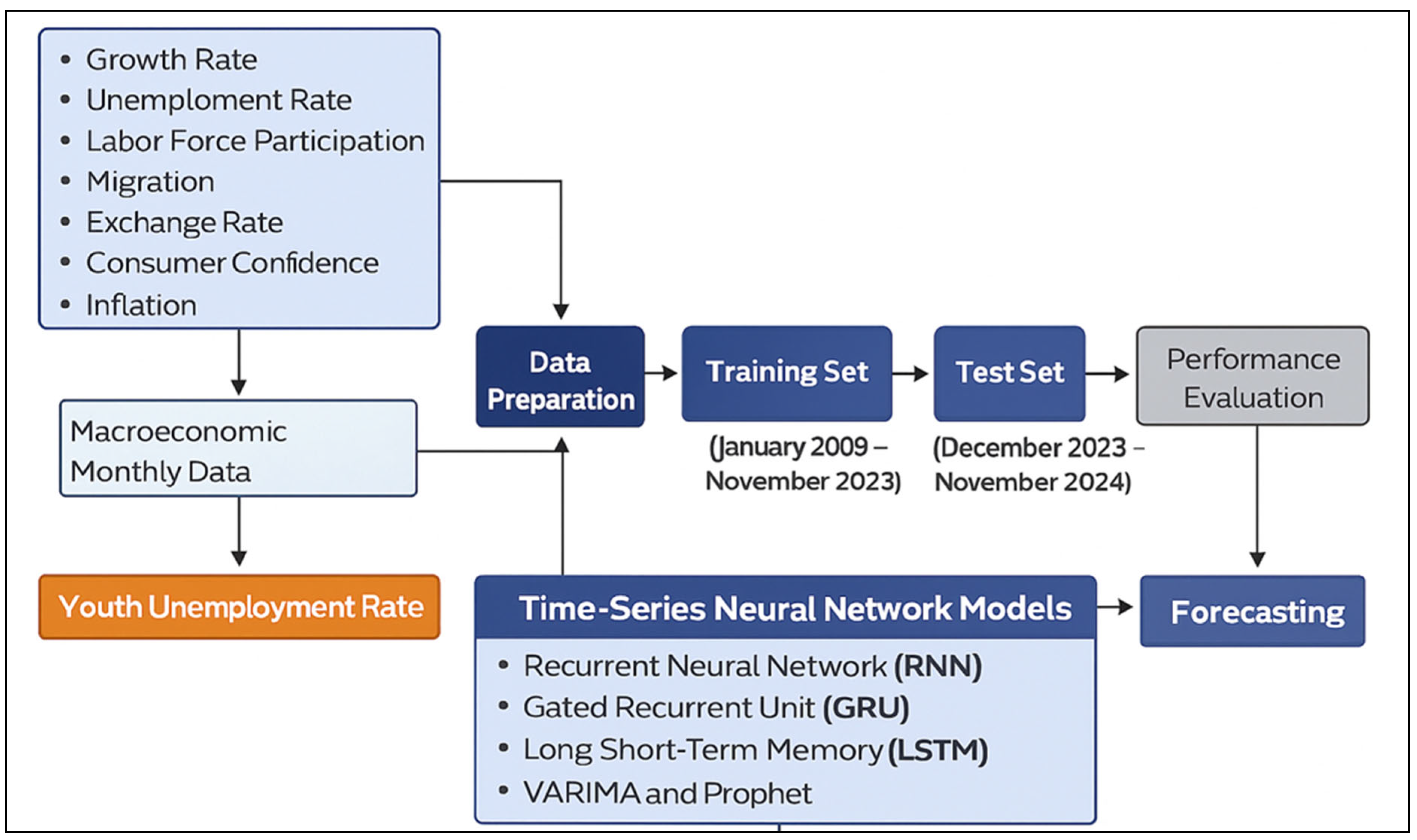
The flow diagram in Figure 1 shows the operation of the youth unemployment prediction model used in the study.

3.2. Recurrent Neural Network (RNN)

A particular type of neural networks called recurrent neural networks (RNNs) was created especially to describe sequential data with temporal dependencies, including voice, spoken language or time series [29]. RNNs, in contrast to feed-forward networks, use both recent and historical inputs to gradually gather contextual data. Different input-output architectures are utilized depending on the job. Many-to-many or many-to-one topologies are frequently chosen for time series forecasting, where the durations of the input and output sequences vary according to the prediction horizon.

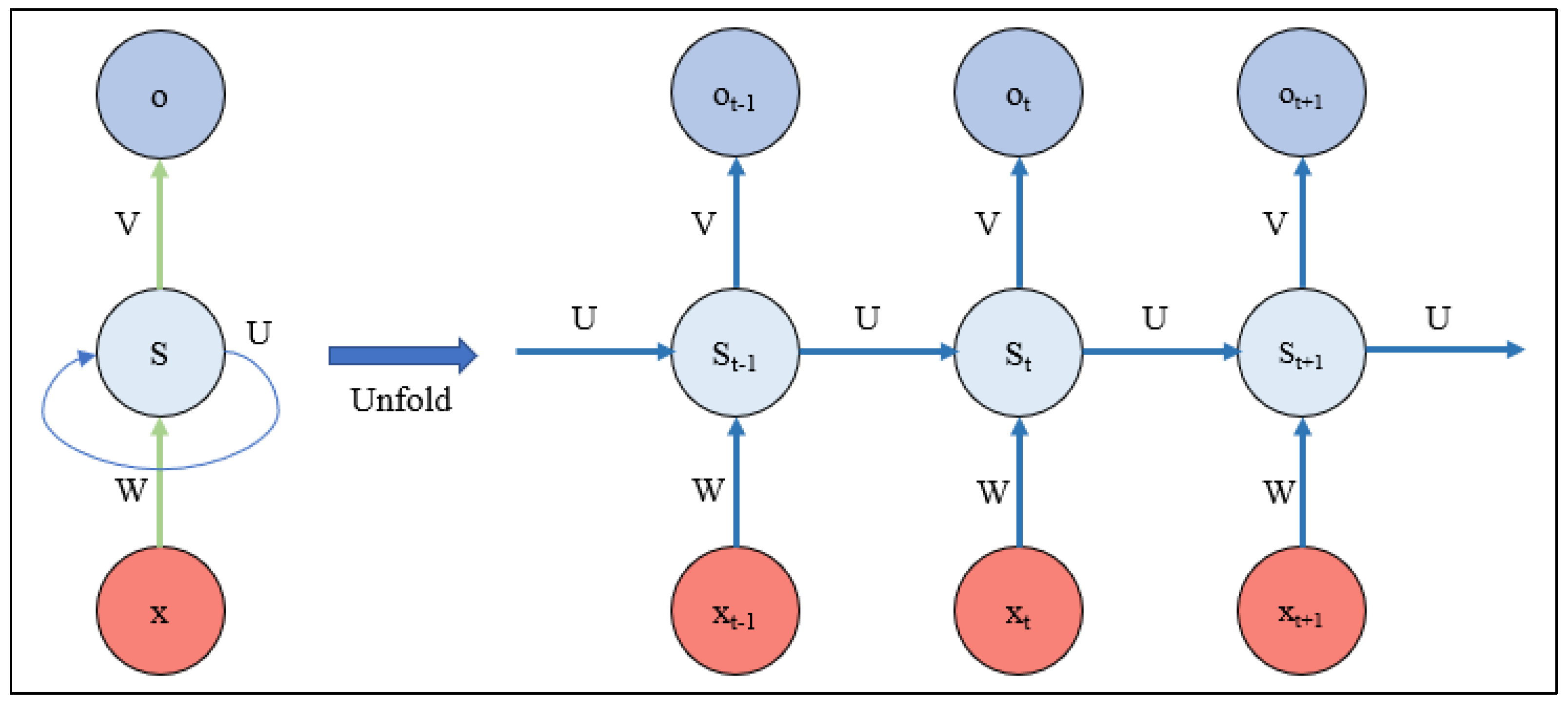
The learning mechanism of RNNs is depicted in Figure 2, where weight changes over time steps add complexity and frequently lead to long-term dependence problems. Equations (1)–(3) demonstrates how the recurrent structure, with self-feedback connections, more closely matches biological neural networks than conventional feed-forward models, giving RNNs greater flexibility when handling variable-length sequences [30].

$$o_t=f\left(x_t\right)$$

(1)

$$o_{t+1}=f\left(x_{t+1}\right)+f\left(o_t\right)$$

(2)

$$o_{t+2}=f\left(x_{t+2}\right)+f\left(o_{t+1}\right)$$

(3)

where o_t denotes the output at time t, and x_t represents the input at the same time step. An RNN cell is represented by Equation (4):

$$S_t=\sigma (W{x}_t+U{S}_{t-1}+\mathrm{b})$$

(4)

Here, S_t denotes the hidden state at time step t; W represents the weight matrix for the current input; U refers to the recurrent weight matrix connecting the previous hidden state; and b is the bias term.

3.3. Gated Recurrent Network (GRU)

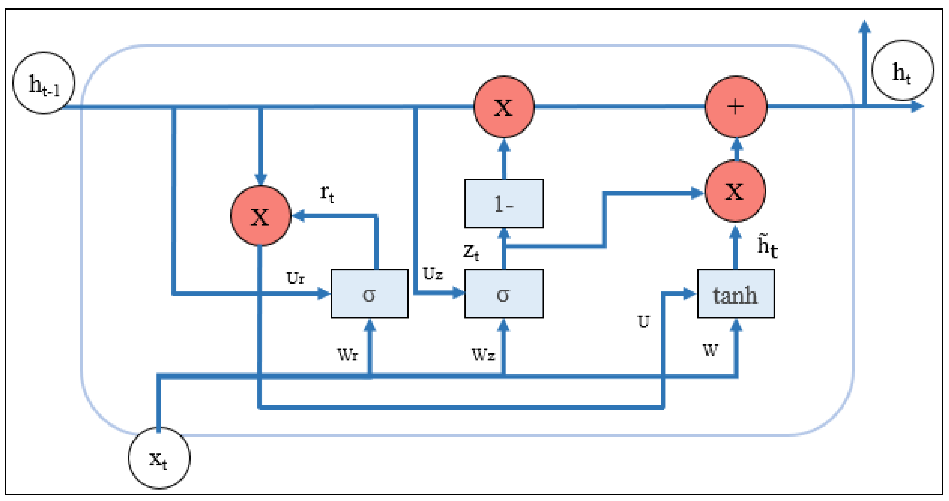
The Gated Recurrent Unit is a prevalent refinement of the RNN, conceived as a more efficient alternative to LSTM architecture [31]. The GRU, similar to LSTM in structure, consolidates the input and forget gates into a singular update gate that governs the preservation of historical knowledge inside the present state. The reset gate regulates the extent to which prior information is integrated with the present input. In contrast to LSTM, the GRU consolidates the cell state and hidden information into a unified representation, hence decreasing the parameter count. This decrease enhances computing efficiency and expedites convergence, frequently without sacrificing predictive accuracy, rendering GRUs a compelling option for practical applications. The architecture of the GRU model is depicted in Figure 3 [32].

The functioning of a GRU cell is governed by the following equations [32]:

$$z_t=\sigma (x_t{W}^z+h_{t-1}{U}^z+b_z)$$

(5)

$$r_t=\sigma (x_t{W}^r+h_{t-1}{U}^r+b_r)$$

(6)

$${\tilde{h}}_t=\mathrm{t}\mathrm{a}\mathrm{n}\mathrm{h} (r_t·h_{t-1}U+x_{t}W+b)$$

(7)

$$h_t=\left(1-z_t\right)·{\tilde{h}}_t+z_t·h_{t-1}$$

(8)

Here, W^z, W^r, and W denote the weight matrices for the input vector, while U^z, U^r, and U correspond to the weight matrices for the previous hidden state. b_z, b_r, and b are bias terms, σ is the sigmoid activation function, and ${\tilde{h}}_t$ is the candidate hidden state. The update gate z_t regulates the balance between preserving past information and incorporating new input, whereas the reset gate r_t determines the degree of dependency on prior hidden states.

3.4. Long Short-Term Memory (LSTM)

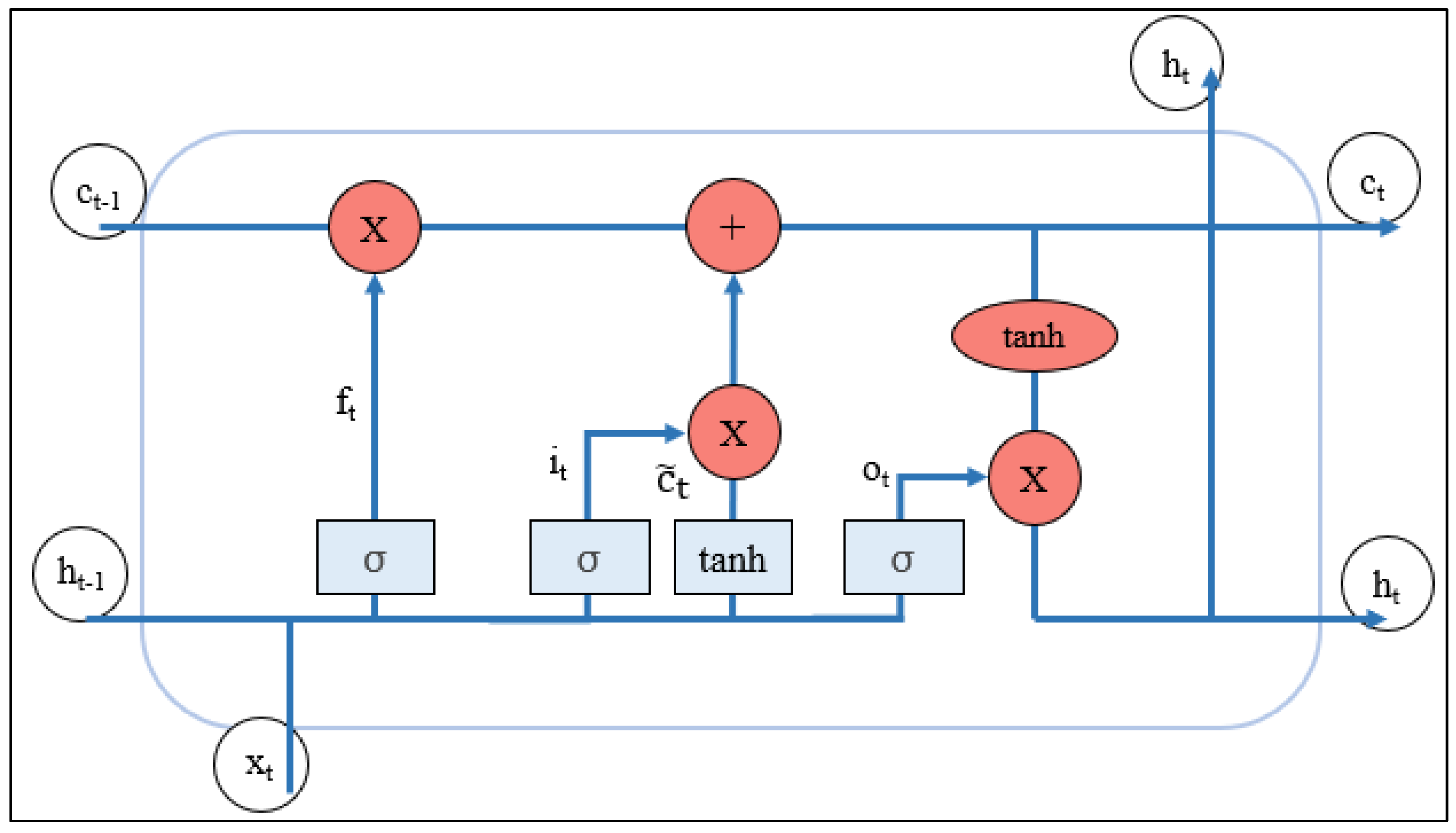
Among several RNN designs, the Long Short-Term Memory network is distinguished by its capacity to efficiently capture long-term dependencies in time series data via its specialized memory cells [33]. Additionally, LSTM forecasting achieves very high accuracy rates [34]. LSTM, initially introduced by Hochreiter and Schmidhuber [35], mitigates the vanishing gradient issue present in conventional RNNs when simulating prolonged temporal contexts. This is accomplished by sustaining a continuous error flow through gated mechanisms input, output, and forget Gates that govern the retention or modification of information inside the network. Thus, LSTM improves traditional RNNs by enabling more precise modeling of relationships with significant temporal intervals. The architecture of the LSTM model is seen in Figure 4.

At time step t, x_t represents the LSTM input, h_t−1 is the previous hidden state, c_t is the current cell state, and h_t is the current hidden state. The computation proceeds as follows [36]:

• Candidate Cell State:

  $${\tilde{c}}_t=\mathrm{t}\mathrm{a}\mathrm{n}\mathrm{h} (W_c·\left[h_{t-1},x_t\right]+b_c)$$

  (9)

  where W_c and b_c are the weight matrix and bias, respectively.
• Input Gate: Controls how much of the candidate cell state is added:

  $$i_t=\mathsf{\sigma }(W_i·\left[h_{t-1},x_t\right]+b_i)$$

  (10)
• Forget Gate: Regulates how much of the previous cell state is retained:

  $$f_t=\mathsf{\sigma }(W_f·\left[h_{t-1},x_t\right]+b_f)$$

  (11)
• Cell State Update:

  $$c_t=f_t·c_{t-1}+i_t{\tilde{c}}_t$$

  (12)
• Output Gate: Determines the hidden state output:

  $$o_t=\mathsf{\sigma }(W_o·\left[h_{t-1},x_t\right]+b_o)$$

  (13)
• Hidden State Calculation:

  $$h_t=o_t·\mathrm{t}\mathrm{a}\mathrm{n}\mathrm{h} \left(c_t\right)$$

  (14)

This architecture enables LSTMs to selectively store, update, and output information over long sequences, effectively mitigating the vanishing gradient problem.

3.5. VARIMA

The VARIMA (Vector Auto-Regressive Integrated Moving Average) model is a forecasting method used for multivariate time series. It combines the univariate structure of the ARIMA model with the VAR (Vector Auto-Regression) approach, which allows multiple variables to be modeled simultaneously. This combines the effects of stationarity, historical values, and error terms. Compared to univariate ARIMA, the joint dynamics among multiple variables provide the generalized power of the model. For highly correlated series (e.g., economic or energy indicators), VARIMA is generally more accurate than single ARIMA. However, if variables are less correlated, similar performance can be achieved with ARIMA [37].

The general ARIMA (p,d,q) model is expressed as:

Φ_p(L) (1 − L)^d y_t = c + Θ_q(L) ε_t

(15)

• y_t: Value of the time series at time t
• L: Lag operator (Ly_t = y_{t − 1})
• d: Number of differences taken to stationarize the series
• Φ_p(L): AR (p-order autoregressive) polynomial
• Θ_q(L): MA (q-order moving average) polynomial
• ε_t: White noise error term (mean 0, constant variance)

3.6. PROPHET

Prophet is a time series forecasting model developed by Facebook (now Meta) and widely used in business and social sciences. It was introduced in a 2017 paper by Sean J. Taylor and Benjamin Letham [38]. The model makes predictions by decomposing time series based on three main elements: the long-term trend (g(t)), seasonality (s(t)), and the effect of holidays or special days (h(t)). Its general mathematical form is as follows:

y(t) = g(t) + s(t) + h(t) + ε_t

(16)

Here, g(t) represents the trend component of the series and can be modeled with piecewise linear or logistic growth functions. The seasonality component, s(t), is defined using Fourier series:

s(t) = Σ [a_n cos(2πnt/P) + b_n sin(2πnt/P)]

(17)

Holidays or special days are added to the model as dummy variables with the term h(t). With this approach, Prophet can flexibly capture trend breaks (change points), multiple seasonality’s, and exogenous shocks. Additionally, its robustness against missing data and outliers makes it particularly useful in business and macro-economic forecasting.

3.7. Evaluation Metrics

Various error assessment measures were employed to compare the basic models with those refined through hyperparameter optimization, owing to the utilization of a regression-based technique. In this context, Mean Squared Error (MSE), Root Mean Squared Error (RMSE), Mean Absolute Error (MAE), Median Absolute Error (MedAE), and Mean Absolute Percentage Error (MAPE) were chosen as metrics for performance evaluation. MAE and MedAE mitigate the influence of outliers and represent central error patterns more equitably; conversely, RMSE allocates greater significance to substantial mistakes, so effectively emphasizing significant discrepancies in the model’s predictions. MAPE enables the comparison of datasets with varying scales by expressing the error rate as a percentage. The mathematical formulations for these error measures are delineated in Equations (18)–(22).

$$MSE={\displaystyle \frac{1}{n}}{\sum }_{i=1}^n{(a_i-p_i)}^2$$

(18)

$$RMSE=\sqrt{{\displaystyle \frac{1}{n}}{\sum }_{i=1}^n{(a_i-p_i)}^2}$$

(19)

$$MAE={\displaystyle \frac{1}{n}}{\sum }_{i=1}^n\left|a_i-p_i\right|$$

(20)

$$MedAE=median(\left|a_1-p_1\right|, \left|a_2-p_2\right|, \dots , \left|a_n-p_n\right|)$$

(21)

$$MAPE={\displaystyle \frac{100\%}{n}}{\sum }_{i=1}^n\left|{\displaystyle \frac{a_i-p_i}{a_i}}\right|$$

(22)

where a_i denotes the actual value, p_i represents the predicted value, and n refers to the total number of observations.

3.8. The Concept of Symmetry and Impact on the Study

In this study, symmetry and asymmetry are treated as analytically distinct properties of multivariate time-series dynamics rather than purely descriptive concepts. Symmetry refers to the presence of stable, proportional, and coordinated co-movements among macroeconomic variables, implying that shocks and adjustments propagate through the system in a balanced and directionally consistent manner. Asymmetry, by contrast, refers to nonlinear, state-dependent, or time-varying responses in which the magnitude and persistence of adjustments differ across periods or shock regimes. From an empirical standpoint, structural symmetry is operationalized through the VARIMA framework. VARIMA captures symmetry by modeling linear interdependencies and mutual lag structures among variables, thereby representing equilibrium-oriented dynamics in which macroeconomic indicators jointly adjust over time. Symmetric behavior is inferred when the model exhibits stable coefficients, low and unbiased forecast errors, and consistent predictive performance across the out-of-sample horizon.

Dynamic asymmetry is operationalized through nonlinear forecasting models, including GRU, LSTM, and Prophet. These models are designed to accommodate nonlinear transformations, regime shifts, and shock-sensitive dynamics. Asymmetry is inferred when such models outperform linear benchmarks during periods of heightened volatility, when forecast errors display temporal heterogeneity, or when predictive accuracy varies across short- and medium-term horizons, indicating uneven adjustment paths. The comparative evaluation of VARIMA and nonlinear models under a unified sampling and preprocessing protocol thus serves as an implicit empirical test of symmetry versus asymmetry. Performance of VARIMA suggests dominance of symmetric structural co-movements, whereas competitive or superior performance of nonlinear models indicates the presence of asymmetric temporal responses. This framework allows symmetry to be defined, measured, and interpreted in a reproducible manner within a forecasting context.

4. Analysis and Results

4.1. Features of the Models

Before modeling using LSTM, RNN or GRU, variables are scaled using Minimum Maximum Scaling (Minmax Scaling) by dividing the difference in each observation with the minimum value and dividing by the difference in minimum and maximum values of the variable and this procedure was only fit on the training set. First a vanilla neural network is used with 2 hidden layers. The first layer consists of either LSTM, RNN or GRU layer with a size of 32 and dropout rate of 0.2. The second layer is the Batch Normalization layer followed by the Dropout layer with a rate of 0.2. Then another LSTM, RNN or GRU layer with a size of 32 and dropout rate of 0.2 is followed by a Dropout layer with a rate of 0.2. The output layer is a Dense layer with 1 neuron without activation function. Adam is the optimization method with a learning rate of 0.001, and Mean Squared Error loss is used. In fitting the model, 20% of the training dataset is used as validation dataset and epoch of 16 and batch size of 16 is used. For the purpose of finding a better model, hyperparameter tuning is used where LSTM, GRU or RNN layers are trained with 32, 64,96 or 128 neurons, dropout rates of 0.2, 0.3, 0.4 or 0.5, activation functions of “ReLU”, “TanH” and “Sigmoid” and Adam and RMSPROP optimizers are used. Model with least validation loss is selected and Bayes Optimization is used to select the best performing parameters from the predefined grid. Since random seeding is preferred to replicate results, since GPU is utilized for training and testing of neural networks, CUDA library’s internal methods avoid replicating same results although random seeding is used.

Auto-regressive integrated moving average (ARIMA) models have been the de facto classical statistical method in time series prediction. It uses univariate series, only one variable is used to model and predict the variable’s future values using autocorrelations in the data. Auto-regressive part (AR) with p parameter models the relationship with the current and past values, moving average (MA) with q parameter part models the relationship between current and past forecast values and integrated (I) part represents the differencing to make the series stationary. To use more than one variable, vector auto-regressive integrated moving average (VARIMA) models have been developed and it captures cross-correlations between several series. By using multiple variables, it can predict the dependent variable’s future values. To use VARIMA, like ARIMA models, first variables are tested if they are stationary using Augmented Dickey–Fuller Test. If they are not stationary, variables are differenced and re-tested. Next, the first 180 observations are used for model training and the last 12 observations for model testing using metrics. Like ARIMA models, p and q values are predetermined before building the model. First a model with p and q value of 1 each is built. Because best performing p and q values are not known, combinations of p and q values are used for model and p and q values of best fitting model with least Akaike Information Criterion is chosen for model building.

For Prophet, like VARIMA, the first 180 observations are used for model training and the last 12 observations for model testing using metrics. We did not use hyperparameter optimization for Prophet model. Model performances are compared after prediction using the test dataset. Mean Squared Error (MSE), Root of Mean Squared Error (RMSE), Mean Absolute Error (MAE), Median Absolute Error (MedAE) and Mean Absolute Percentage of Error (MAPE) are used as performance metrics. MSE is the sum of differences between actual and predicted errors and RMSE is the square root of MSE. MAE is the average of absolute differences between predicted and actual values. MedAE is the median of absolute differences between predicted and actual values while MAPE is the percentage error relative to actual value.

In addition, Models are built, tested and performance metrics are calculated using Python version 3.11.5, TensorFlow version 2.17.0, stats model version 0.14.0 and Prophet version 1.1.7 on an IBM compatible PC with Ubuntu version 22.04.5. The dataset consisted of 192 observations and 8 variables. Youth unemployment variable is the target variable while the rest are predictors.

4.2. Statistical Data on the Variables Used in the Models

This section presents some statistical data related to the variables used in the study. Additionally, the cointegration test data for the dependent and independent variables, which form the basis of the study, and the parameter optimization data applied to the models are shown. Descriptive statistics of variables are listed in

Table 2. Descriptive statistics of variables.

Variable	Mean	Standard Deviation	Min–Max	1st Quartile 3rd Quartile
Economic Growth	2.59	4.97	−14.54–16.40	0.50–4.61
Unemployment	10.94	1.75	8.00–16.12	9.63–12.15
Labor Force Participation Rate	45.05	4.01	34.00–51.20	41.70–48.90
Migration	33,636.05	85,460.50	−60,4492.0–263,955.0	6304.50–52,739.50
Exchange Rate	7.31	8.73	1.43–34.24	1.82–7.58
Consumer Confidence Index	85.28	7.41	63.40–97.40	79.80–91.77
Inflation	1.50	2.00	−1.44–13.58	0.41–1.95
Youth Unemployment	17.41	5.28	8.0–27.40	13.05–20.80

that reports the descriptive statistics of the variables used in the multivariate forecasting framework, providing an initial overview of their distributional properties, variability, and potential sources of asymmetry. These statistics are critical for understanding the structural characteristics of the data prior to econometric and machine learning modeling.

When the mean values in Table 2 are examined, it is seen that youth unemployment (17.41%) is generally higher than overall unemployment (10.94%). This demonstrates the difficulties experienced by the young workforce in Turkey in finding employment. The high standard deviation value in the migration data is interpreted as an indicator that Turkey faces irregular migration flows. The migration variable should be evaluated specifically for Turkey. Economic growth exhibits a relatively low mean value (2.59) but a high standard deviation (4.97), together with a wide range spanning from −14.54 to 16.40. This indicates substantial macroeconomic volatility over the sample period, reflecting pronounced contractionary and expansionary phases.

The general unemployment rate displays comparatively lower dispersion, with a mean of 10.94 and a standard deviation of 1.75. The interquartile range (9.63–12.15) indicates a relatively stable distribution, suggesting that overall unemployment evolves more smoothly than youth unemployment. Labor force participation shows moderate variability, with a mean of 45.05 and a standard deviation of 4.01. The relatively wide min–max range (34.00–51.20) points to structural shifts in labor market engagement, which may interact with youth unemployment dynamics both symmetrically in the long run and asymmetrically during adjustment periods.

Migration exhibits the highest volatility among all variables. The very large standard deviation (85,460.50) and the wide range, including substantial negative and positive values, indicate strong and irregular migration flows. Due to the situation in Syria, the number of migrants has increased significantly through Turkey’s migrant admission agreements, along with EU support.

Exchange rates also display pronounced dispersion, with a standard deviation (8.73) exceeding the mean (7.31) and a wide range from 1.43 to 34.24. Consumer confidence exhibits comparatively moderate variability, indicating cyclical but smoother fluctuations. Inflation, while having a relatively low mean (1.50), shows episodic spikes, as reflected in its range (−1.44 to 13.58), suggesting nonlinear adjustment patterns.

Overall, the descriptive statistics reveal pronounced heterogeneity and asymmetry across variables, providing strong empirical motivation for the study’s multivariate and symmetry-aware forecasting framework.

In addition, in this study, Augmented Dickey–Fuller (ADF) and Phillips–Perron (PP) tests were applied for stationarity testing. Commonly used criteria in the literature for determining the common lag length for variables in the equation system include Final Prediction Error (FPE), Hannan–Quinn (HQ), Schwarz (SW), Likelihood Ratio (LR), and Akaike Information Criteria (AIC). Lag length was determined according to these criteria. Bayer-Hanck [38], Cointegration Analysis was used to investigate the long-term relationship. Also, long-term correlation coefficients were found using FMOLS and DOLS. Finally,

Table 3. Definition of Variables Used in the Analysis.

Variables	Symbols	Definition
Youth Unemployment Rate	YUR	Dependent Variable
Inflation	INF	Independent Variable
Labor Force Participation Rate	LFP	Independent Variable
Growth Rate	GR	Independent Variable
Migration	MIG	Independent Variable
Exchange Rate	ER	Independent Variable
Consumer Confidence	CC	Independent Variable
Unemployment Rate	UR	Independent Variable

shows that dependent and independent variables.

The variables were found to be stationary for the first-order difference, and stationarity was achieved at the I (1) level. Lag lengths were determined for cointegration analysis. According to the Final Prediction Error (FPE), Hannan–Quinn (HQ), Schwarz (SW), Likelihood Ratio (LR) and Akaike Information Criteria (AIC) criteria, a lag of “1” was found to be appropriate. In this case, cointegration analysis will be performed with the first-order differences in the variables and a lag length of 1. All series were seasonally adjusted using the Census X-13ARIMA-SEATS procedure to remove deterministic and stochastic seasonal effects.

Bayer and Hanck [38], noting the contradictory results of cointegration tests in the literature, developed a new test that combines the cointegration tests of Engle and Granger [39], Boswijk [40], and Banerjee et al. [41]. Combining the probability values (significance levels) of these tests and arriving at a more robust cointegration test, Bayer and Hanck’s [38] cointegration test utilizes the probability values of Engle-Granger’s [39] single-equation test, Johansen’s [42] multi-equation test, Boswijk’s [40] error correction term-based test, and Banerjee et al.’s [41] test.

Table 4. Long-Term Cointegration Coefficient Estimates.

	FMOLS	DOLS
Variables	β	β
∆INF	0.098 *	0.090 *
∆LFP	0.085 *	0.079 *
∆GR	−0.106 *	−0.101 *
∆MIG	0.046 *	0.038 *
∆ER	0.085 *	0.079 *
∆CC	−0.096 *	−0.092 *
∆UR	−0.092 *	−0.091 *

* 0.05 is a statistically significant variable.

shows the results of the cointegration test.

During FMOLS and DOLS analyses, autocorrelation and heteroskedasticity issues were addressed using the Newey-West method. No assumption bias was observed during the hypothesis testing. Growth and inflation were found to be the most influential variables on youth unemployment. Furthermore, the cointegration test reveals the degree to which the dependent and independent variables are related to each other. This is a crucial step for assessing the accuracy of the model’s predictions.

Table 5. Vanilla Model and hyperparameter tuned model specifications.

	Model Layers
Vanilla Model	First layer: LSTM, Units = 32, Dropout rate 0.2, activation = TanH Second Layer: Batch Normalization Third Layer: Dropout rate 0.2 Fourth Layer: LSTM, Units = 32, Dropout rate 0.2 Fifth Layer: Dropout rate 0.2 Optimizer: Adam
Tuned LSTM Model	First layer: LSTM, Units = 32, Dropout rate 0.3, activation = TanH Second Layer: Batch Normalization Third Layer: Dropout rate 0.3 Fourth Layer: LSTM, Units = 96, Dropout rate 0.30, activation = ReLU Fifth Layer: Dropout rate 0.2 Optimizer: RMSPROP
Tuned RNN Model	First layer: RNN, Units = 32, Dropout rate 0.2, activation = TanH Second Layer: Batch Normalization Third Layer: Dropout rate 0.3 Fourth Layer: LSTM, Units = 128, Dropout rate 0.4, activation = ReLU Fifth Layer: Dropout rate 0.2 Optimizer: RMSPROP
Tuned GRU Model	First layer: RNN, Units = 32, Dropout rate 0.4, activation = TanH Second Layer: Batch Normalization Third Layer: Dropout rate 0.2 Fourth Layer: LSTM, Units = 96, Dropout rate 0.2, activation = ReLU Fifth Layer: Dropout rate 0.3 Optimizer: RMSPROP

shows that parameter optimization values applied to the models used in the study.

Hyperparameter optimization was used to increase the number of neurons in layers, experiment with different activation functions, and diversify optimization algorithms. These modifications were aimed at improving the accuracy and performance of the models, with more successful results being achieved, particularly in the LSTM and GRU architectures. The most critical implication of the table is that deep learning architectures, beyond classical statistical methods, also possess parametric sensitivity. The main reason for employing hyperparameter optimization in this study is that the prediction performance of deep learning models is highly sensitive to parameter settings. In particular, the number of neurons, activation functions, and optimization algorithms directly affect the model’s ability to capture long-term dependencies in time series data. For example, experimenting with tanh and ReLU activation functions in the LSTM model aims to both capture nonlinear relationships and mitigate gradient vanishing problems. Similarly, comparing the Adam and RMSProp optimizers aims to test the stability of the learning process. The results

Table 6. Performance metrics of models.

	MSE	RMSE	MAE	MedAE	MAPE
Raw LSTM Model	31.10	5.57	4.90	4.90	0.290
Tuned LSTM Model	7.82	2.80	2.57	2.48	0.156
Raw RNN Model	33.21	5.76	5.60	5.55	0.349
Tuned RNN Model	39.68	6.29	6.08	5.78	0.372
Raw GRU Model	21.42	4.63	4.51	4.51	0.275
Tuned GRU Model	68.71	8.29	8.23	8.05	0.505
Prophet	3.45	1.86	1.50	1.39	0.091
VARIMA (p = 1, q = 1)	0.02	0.15	0.15	0.14	0.009
VARIMA (p = 2, q = 0)	0.02	0.13	0.12	0.10	0.007

shows that hyperparameter optimization significantly reduced error rates in the LSTM model (MAPE decreased from 0.290% to 0.156%). This finding highlights the critical role of appropriate parameter selection in predicting highly volatile macroeconomic indicators such as youth unemployment. Conversely, the decrease in prediction accuracy due to optimization in the RNN model stems from the fact that this architecture cannot capture long-term dependencies as effectively as LSTM and GRU. Therefore, the impact of hyperparameter optimization varies depending on the model architecture.

4.3. Model Performance Metrics

Table 6 reports the out-of-sample forecasting performance of all models using multiple error metrics, including MSE, RMSE, MAE, MedAE, and MAPE. The use of complementary accuracy measures allows for a robust evaluation of predictive performance by capturing both average error magnitude and relative percentage deviations. The results reveal substantial performance heterogeneity across model classes. Among the deep learning approaches, raw RNN and raw LSTM models exhibit relatively high error levels across all metrics, indicating limited generalization capability in a small-sample macroeconomic context. Although hyperparameter tuning improves the performance of the LSTM model considerably reducing RMSE from 5.57 to 2.80 and MAPE from 0.290 to 0.156—the tuned LSTM remains clearly inferior to both Prophet and VARIMA. In contrast, tuning does not yield performance gains for the RNN and GRU architectures; the tuned RNN and tuned GRU models perform worse than their raw counterparts, suggesting overfitting and unstable parameter learning when model complexity is increased.

The raw GRU model performs better than raw RNN and LSTM specifications, supporting the view that GRU’s more parsimonious gating structure is relatively better suited to macroeconomic time series. However, The Prophet model demonstrates strong and stable performance, achieving low error values across all metrics (RMSE = 1.86, MAE = 1.50, MAPE = 0.091). This result reflects Prophet’s ability to flexibly accommodate trend changes and localized irregularities while maintaining reasonable forecast stability.

The most striking result emerges from the VARIMA models, which clearly outperform all competing approaches by a wide margin. Both VARIMA specifications yield exceptionally low error values, with RMSE as low as 0.13 and MAPE below 1%. The VARIMA (p = 2, q = 0) specification achieves the best overall performance, marginally improving upon the VARIMA (p = 1, q = 1) model across all metrics. This superior accuracy indicates that the linear multivariate structure of VARIMA successfully exploits long-run equilibrium relationships and coordinated co-movements among macroeconomic variables and youth unemployment. Here, the results strongly support the study’s central argument. Following plots for model prediction of the models are shown in Figure 2, Figure 3, Figure 4 and Figure 5.

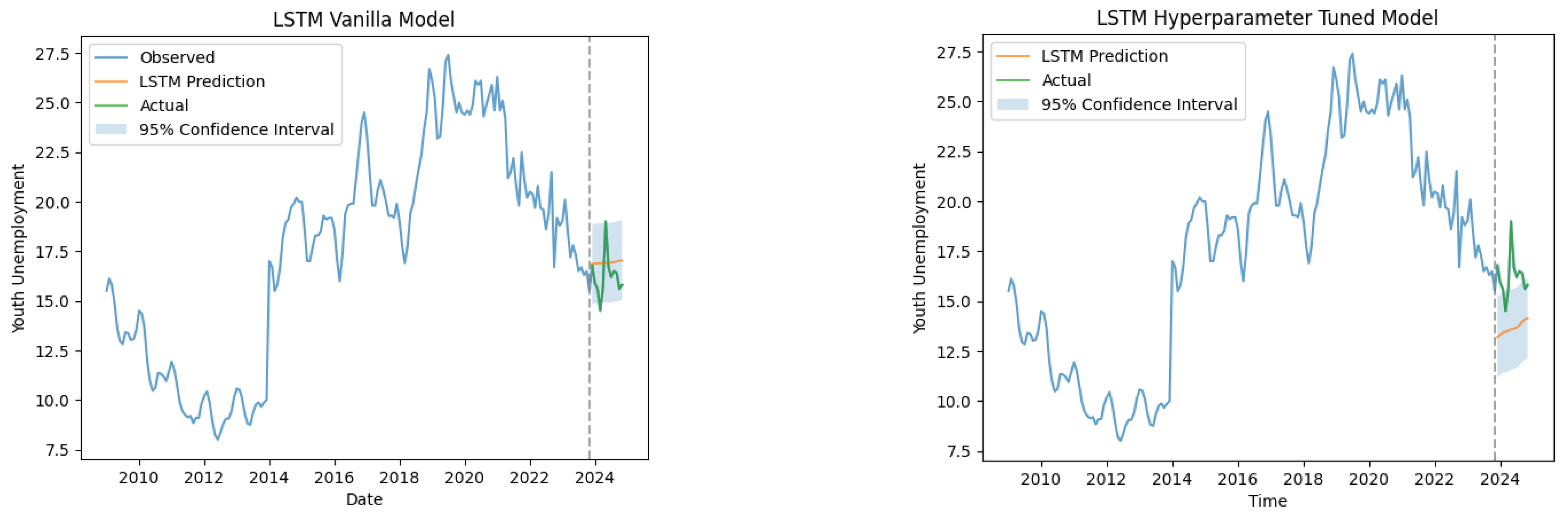
Figure 5 illustrates the forecasting behavior of the LSTM model before and after hyperparameter optimization, thereby providing direct visual evidence of how model tuning affects predictive performance in a small-sample macroeconomic setting. In the vanilla LSTM specification (left panel), the model generates relatively smooth forecasts that partially track the observed youth unemployment series during the test period. However, the predictions exhibit limited responsiveness to short-term fluctuations and tend to underestimate the magnitude of observed changes. On the other hand, following hyperparameter optimization (right panel), the LSTM model displays improved short-term adaptability, with forecasts that adjust more visibly to recent movements in youth unemployment. The optimized model captures directional changes more effectively than the vanilla specification, indicating that tuning enhances the model’s sensitivity to local temporal patterns. Nevertheless, despite these improvements, the tuned LSTM still exhibits systematic deviations from the realized values, particularly at the beginning of the test period, and the confidence intervals remain relatively wide.

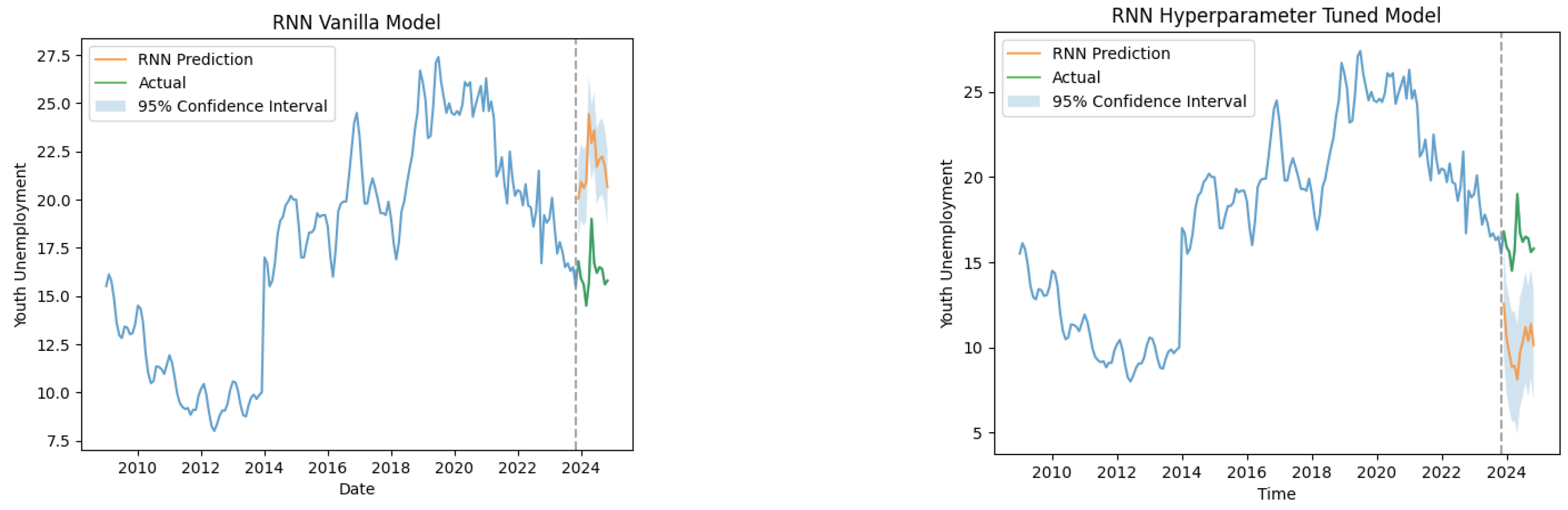
Figure 6 compares the forecasting performance of the vanilla and hyperparameter-tuned RNN models in the same period. In the vanilla specification, the RNN model exhibits pronounced forecast instability, with predictions deviating substantially from the observed youth unemployment series and displaying excessive sensitivity to recent observations. This behavior indicates limited capacity to capture the underlying temporal structure of the data. Following hyperparameter tuning, the RNN model shows marginal improvement in short-term responsiveness; however, the tuned specification still produces systematically biased forecasts and wide confidence intervals. The deterioration in performance after tuning further suggests overfitting and unstable parameter learning in a small-sample macroeconomic context.

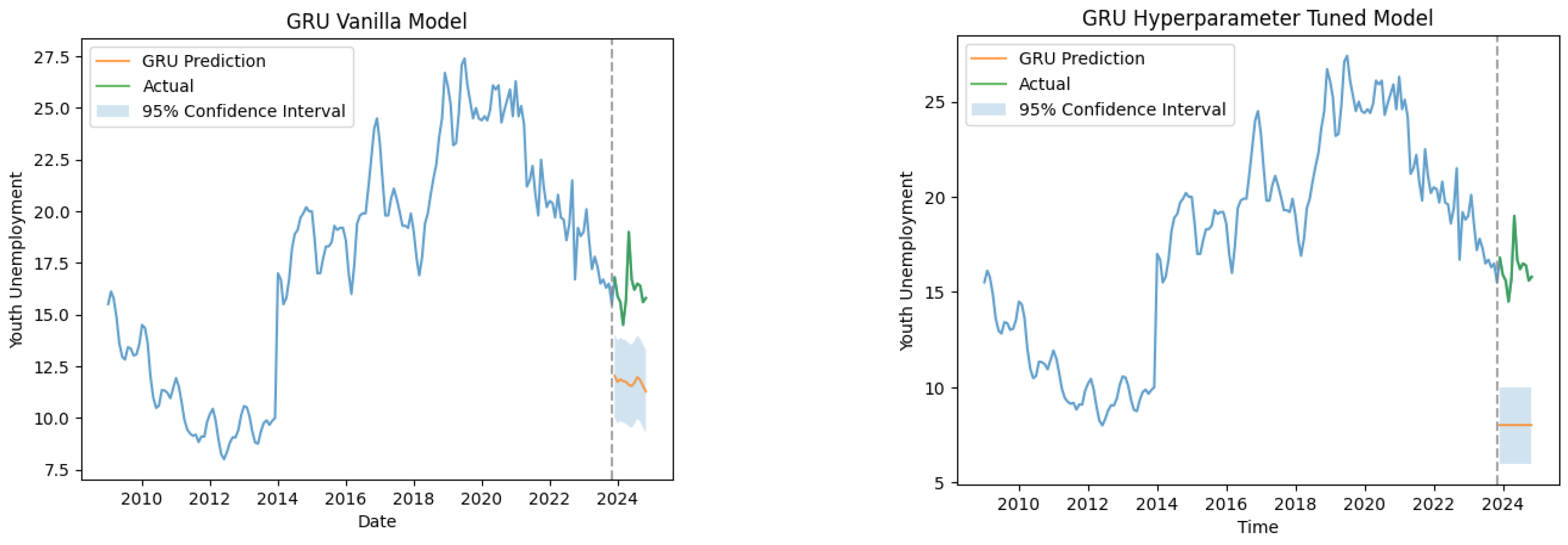
Figure 7 presents forecasting performance of the vanilla and hyperparameter-tuned GRU models. In the vanilla specification, the GRU model generates relatively smooth forecasts but systematically underestimates the level of youth unemployment during the test period, indicating limited sensitivity to recent structural changes. Although the confidence interval captures part of the observed variation, the point forecasts remain biased downward. Following hyperparameter tuning, the GRU model exhibits a sharper and more abrupt adjustment at the beginning of the test period, resulting in pronounced deviations from the observed values and wider uncertainty bands. This deterioration in performance after tuning suggests that increased model flexibility amplifies overfitting rather than improving generalization in a small-sample macroeconomic setting.

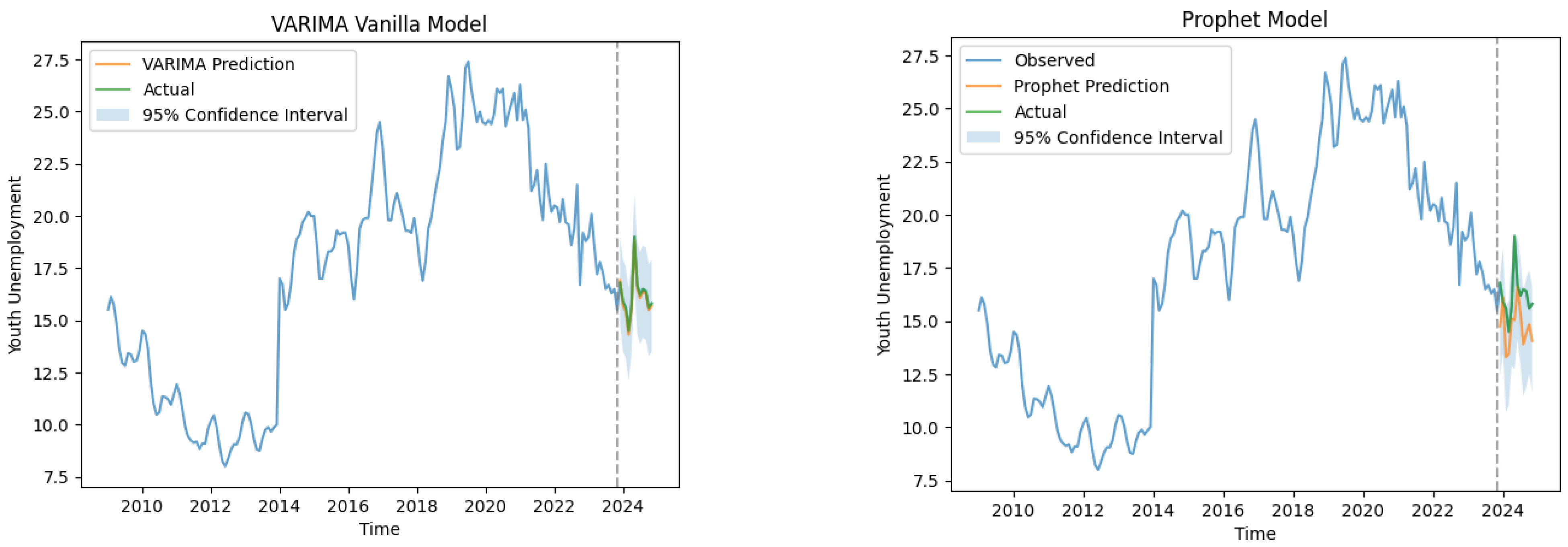
Figure 8 presents the trend of the youth unemployment rate over time and compares the prediction performance of two different modeling paradigms (VARIMA and Prophet) on the same test period. The vertical dashed line clearly shows the separation between the training and test periods, thus visually confirming that all predictions are truly out-of-sample.

Firstly, the VARIMA model robustly captures both historical trends and intervaried relationships. VARIMA’s prediction values almost matched actual observations, especially during the test period. This result also directly supports the econometric equivalent of the “symmetric co-movements” concept, one of the main claims of the paper. VARIMA’s linear and multivariate structure represents equilibrium-adjusting dynamics between macroeconomic indicators and youth unemployment; this ensures that prediction errors remain limited and balanced during the test period. This methodologically justifies the use of VARIMA as a reference model representing structural symmetry. As a result, multivariate time series methods are expected to provide more consistent accuracy in predicting youth unemployment compared to deep learning methods.

On the other hand, Prophet model successfully captures trend breaks and seasonality. Prophet forecasts are observed to be quite close to actual values, reinforcing the model’s practical applicability. Furthermore, the model’s flexible structure allows it to adapt to sudden fluctuations. This demonstrates Prophet’s utility in forecasting macroeconomic indicators such as youth unemployment and its potential as a reliable short-term forecasting tool for policymakers. Moreover, the fact that predictions sometimes fall below or above actual values, and the widening confidence intervals, indicate that the model exhibits time-varying, regime-sensitive, and asymmetric responses.

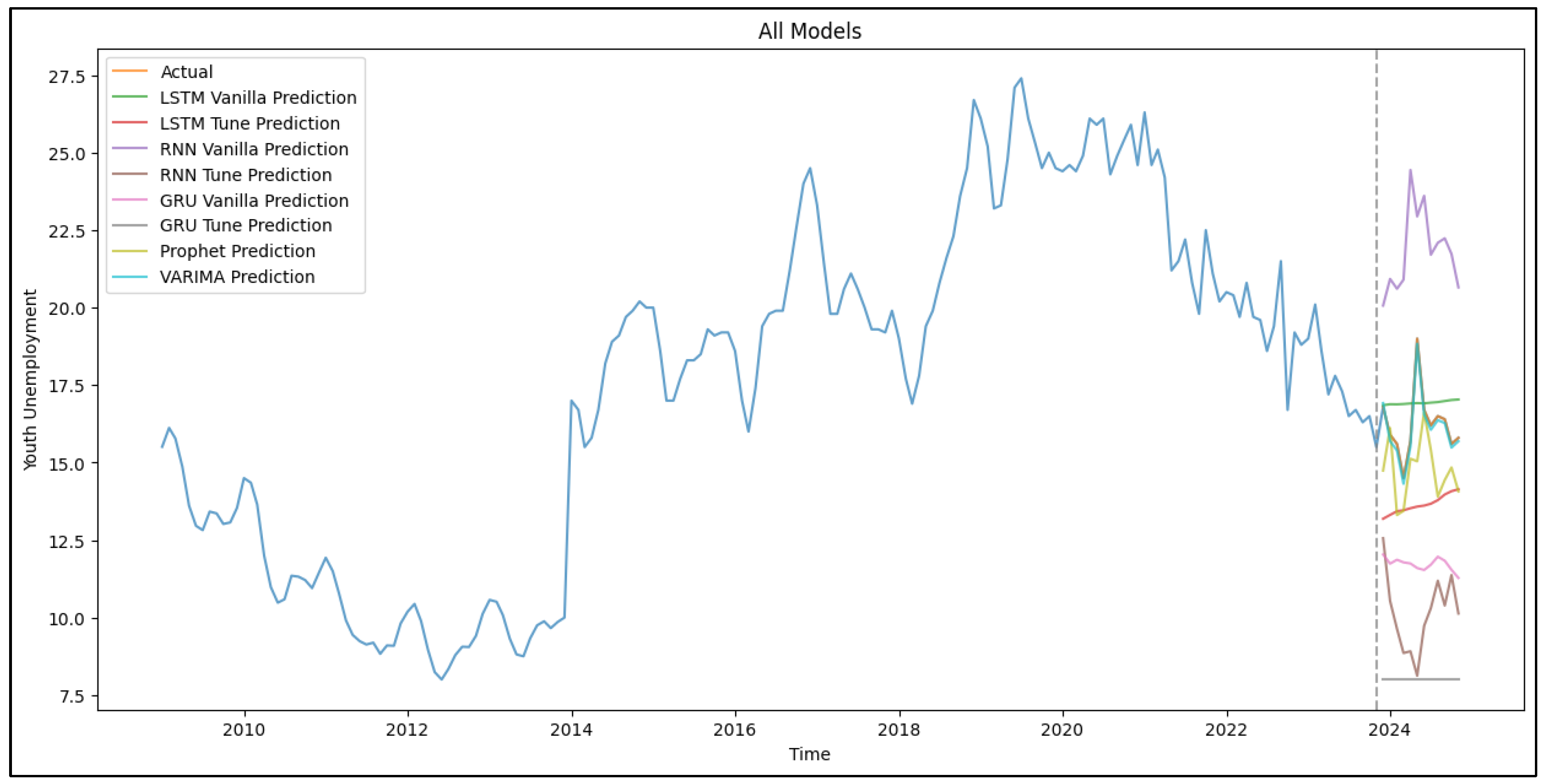
Figure 9 presents a comparative overview of the forecasting performance of all models employed in the study, including VARIMA, Prophet, and both vanilla and tuned versions of RNN, LSTM, and GRU architectures. The dashed vertical line clearly marks the transition from the training period to the out-of-sample test period, ensuring that all predictions shown in the final segment represent genuine forecasts rather than in-sample fits. The historical trajectory of youth unemployment prior to the test period is characterized by pronounced cyclical movements and structural shifts, reflecting the influence of macroeconomic volatility, labor market dynamics, and external shocks. This complexity provides a demanding environment for forecasting, particularly given the relatively short out-of-sample horizon.

During the test period, distinct differences emerge across model classes. The VARIMA model produces forecasts that closely track the observed youth unemployment values, exhibiting smooth adjustments and limited dispersion. This stability indicates that the linear multivariate structure of VARIMA effectively captures coordinated co-movements and long-run equilibrium relationships among macroeconomic variables and youth unemployment. As such, VARIMA reflects predominantly symmetric, equilibrium-oriented dynamics. The Prophet model demonstrates more adaptive behavior, responding flexibly to local changes in the series. While this flexibility allows Prophet to capture short-term fluctuations more effectively than some neural network models, it also results in greater variability and occasional deviations from the realized values, positioning Prophet between linear econometric models and fully nonlinear approaches.

In contrast, the deep learning models display substantial heterogeneity. Vanilla RNN and LSTM models perform relatively poorly in the test period, often producing unstable forecasts that systematically under- or overestimate youth unemployment. These results highlight the challenges of applying complex neural architectures to small macroeconomic datasets, where overfitting and limited generalization are significant concerns. Hyperparameter tuning improves performance for some specifications, but instability remains evident, particularly for RNN and LSTM models.

Among the nonlinear approaches, the GRU models especially the tuned version exhibits comparatively better alignment with observed values. Their more parsimonious structure appears better suited to capturing short-term asymmetries without excessive forecast volatility. Overall, the figure supports the study’s central argument that linear multivariate models excel under symmetric equilibrium dynamics, while nonlinear models capture asymmetric temporal behaviors with varying degrees of stability.

5. Discussion

The findings of this study contribute to the growing literature on youth unemployment forecasting by explicitly positioning the results within a comparative methodological framework that integrates econometric and deep learning approaches. In contrast to a substantial portion of prior research that relies on univariate time series models or limited sets of explanatory variables (e.g., ARIMA- or SARIMA-based studies), this study adopts a fully multivariate perspective, incorporating macroeconomic indicators such as economic growth, inflation, labor force participation, migration flows, exchange rate dynamics, and consumer confidence. This design allows for a richer representation of youth unemployment dynamics and aligns with recent calls in the literature for more comprehensive, data-driven forecasting frameworks.

From a comparative standpoint, the strong performance of the VARIMA model in this study is consistent with earlier econometric evidence suggesting that multivariate linear models remain highly competitive when forecasting labor market indicators characterized by coordinated macroeconomic co-movements. Previous studies focusing on Europe and emerging economies report that VAR or ARIMA type models often perform well in environments where unemployment dynamics are closely linked to broader macroeconomic conditions, particularly during periods of relative structural stability. Our results reinforce these findings by showing that the VARIMA (p = 2, q = 0) specification achieves the lowest forecasting errors among all tested models, indicating that youth unemployment in Turkey exhibits a pronounced degree of symmetric interdependence with key macroeconomic variables.

At the same time, the comparative evaluation highlights important differences relative to studies that emphasize machine learning and deep learning methods. Recent research employing recurrent neural networks, GRU, LSTM, or ensemble learning approaches frequently reports superior performance under nonlinear dynamics, structural breaks, or short-term volatility. In line with this strand of the literature, our results show that GRU and Prophet models achieve competitive error rates, particularly in short- and medium-term forecasts. This finding corroborates earlier evidence that GRU architectures, due to their parsimonious gating mechanisms and reduced parameterization, can outperform more complex LSTM structures in macroeconomic forecasting tasks where data length is moderate and volatility is high.

A key contribution of this study lies in moving beyond a purely performance-based comparison and offering an interpretive framework grounded in symmetry and asymmetry. While previous comparative studies typically report error metrics without explaining why certain models perform better, our results suggest that model performance is closely linked to the type of temporal dependence being captured. The superior accuracy of VARIMA reflects its ability to model symmetric co-movements and equilibrium-adjusting dynamics among macroeconomic variables. In contrast, the relatively strong performance of GRU and Prophet highlights their capacity to capture asymmetric and nonlinear responses to shocks, such as abrupt exchange rate movements or migration-related disturbances. This symmetry–asymmetry distinction provides a conceptual bridge between econometric interpretability and machine learning flexibility, which is largely absent from existing youth unemployment forecasting studies. The Turkish case further differentiates this study from much of the existing literature. While many prior contributions focus on advanced economies or rely on cross-sectional or annual data, this study employs a long monthly dataset for an emerging economy characterized by recurrent external shocks, high inflation volatility, and significant migration pressures. The empirical finding that migration and exchange rate volatility play central roles in youth unemployment dynamics extends earlier studies that primarily emphasize growth and general unemployment, and it underscores the importance of incorporating external and behavioral macroeconomic factors into forecasting models for emerging markets.

From a policy perspective, the comparative results suggest that no single modeling paradigm is universally dominant. Econometric models such as VARIMA are well suited for medium- to long-term planning and structural analysis, where symmetric macroeconomic relationships prevail. In contrast, deep learning models—particularly GRU and Prophet—offer practical advantages for short-term monitoring and early warning systems, where asymmetric shock responses are more pronounced. This complementarity echoes recent arguments in the forecasting literature that hybrid or ensemble perspectives may be more informative than model competition alone.

Overall, by systematically comparing econometric and deep learning approaches under a unified, leakage-safe evaluation design and interpreting the results through a symmetry-based lens, this study advances the literature in both methodological and conceptual terms. It demonstrates that youth unemployment forecasting is not merely a technical prediction problem but also a structural analytical challenge, where understanding the balance between symmetric macroeconomic co-movements and asymmetric shock-driven adjustments is essential for both scientific inference and effective policy design.

6. Conclusions

This study aimed to forecast youth unemployment in Turkey by integrating classical econometric approaches, primarily VARIMA and Prophet with advanced deep learning architectures such as RNN, GRU, and LSTM. The findings reveal that multivariate models, particularly the VARIMA (p = 2, q = 0) specification, provide the highest predictive accuracy, demonstrating that youth unemployment dynamics exhibit a strong degree of structural symmetry, with key macroeconomic variables including economic growth, inflation, labor force participation, migration flows, exchange rate movements, and consumer confidence. These results highlight that youth unemployment does not evolve independently but instead follows symmetrical co-movements and balanced interactions with broader macroeconomic conditions. In this sense, the VARIMA framework effectively uncovers the underlying equilibrium structure of the system, in which fluctuations propagate across variables in coordinated and interdependent patterns.

At the same time, the deep learning models employed in this study reveal a complementary layer of asymmetric temporal behavior, particularly in response to sudden shocks or nonlinear structural adjustments. GRU and Prophet outperform other neural architectures by capturing these asymmetric deviations, which often arise when macroeconomic volatility disrupts the otherwise symmetrical relationships within the system. This duality where symmetric structural co-movements coexist with asymmetric shock responses provides deeper insight into the nature of youth unemployment, positioning it as a phenomenon shaped simultaneously by systemic balance and dynamic instability.

From a policy perspective, recognizing these symmetric and asymmetric patterns is essential for designing resilient and adaptive labor market strategies. Symmetric relationships imply that stabilizing macroeconomic fundamentals—such as exchange rate management or migration policy can produce proportionate and predictable improvements in youth employment outcomes. Conversely, the asymmetric responses identified through deep learning models suggest that targeted interventions are necessary during periods of heightened volatility to mitigate uneven or delayed labor market adjustments faced by young workers. This dual policy lens acknowledges that while structural equilibrium can be reinforced through conventional macroeconomic stabilization, asymmetric vulnerabilities require more agile, context-specific mechanisms. The study also contributes theoretically by framing youth unemployment forecasting as a symmetry-informed analytical problem, demonstrating how econometric and deep learning approaches uncover different dimensions of equilibrium, proportionality, and directional dependence within complex socio-economic systems. Future research could enrich this symmetry-based framework by integrating micro-level asymmetries such as regional disparities, education employment mismatches, and sector-specific dynamics as well as exploring cross-country comparisons to assess whether the symmetry patterns observed in Turkey generalize to similar economies.

In conclusion, this study shows that accurate forecasting of youth unemployment emerges from the combined understanding of symmetric macroeconomic co-movements and asymmetric shock-driven behaviors, offering a holistic analytical orientation that aligns closely with the thematic expectations of the Symmetry journal. By merging methodological rigor with a symmetry-focused conceptual lens, the research provides meaningful contributions to both labor market forecasting and the broader interdisciplinary discourse on structural equilibrium and system dynamics.