A BSMOTE-OOA-SuperLearner Hybrid Framework for Interpretable Prediction of Pillar Stability

Abstract

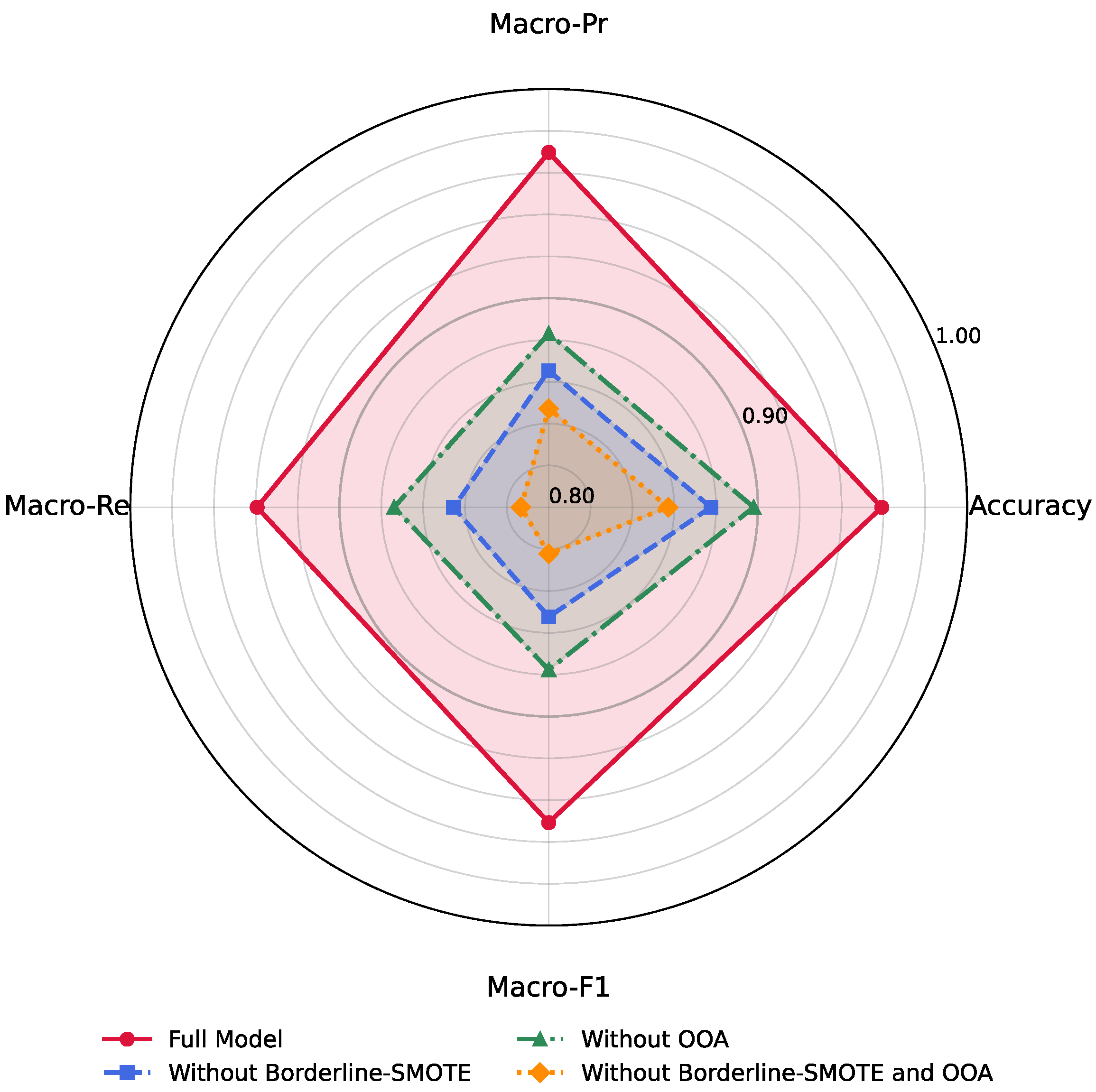
Pillar stability prediction is essential for underground mining safety, yet it remains challenging due to limited data, class imbalance, and insufficient interpretability. This study proposes an integrated Borderline-SMOTE-Osprey Optimization Algorithm-Super Learner framework (BSMOTE-OOA-SL) for hard-rock pillar stability prediction. The framework combines five heterogeneous base learners (ANN, GBDT, KNN, RF, and SVM), applies Borderline-SMOTE within training folds to alleviate class imbalance, and employs the Osprey Optimization Algorithm (OOA) for systematic hyperparameter optimization. The model is evaluated using a dataset of 241 pillar cases from seven underground mines. Statistical experiments based on multiple random train–test splits show that the proposed framework consistently outperforms individual base learners in terms of Accuracy, Macro-Precision, Macro-Recall, and Macro-F1, demonstrating improved robustness and generalization. Ablation results indicate that the joint use of Borderline-SMOTE and OOA leads to quantitative performance gains of 10.21%, 12.25%, 12.61%, and 12.86% in Accuracy, Macro-Precision, Macro-Recall, and Macro-F1, respectively. Under a representative data split, the model achieves an overall accuracy of 95.92%, with strong class-wise Precision, Recall, and F1-score across all stability categories, and AUC values exceeding 0.9 for all classes (reaching 1.0 for the Failed category). SHAP-based interpretability analysis identifies stress-related indicators—particularly average pillar stress, Stress/UCS ratio, and UCS—as the dominant factors governing pillar stability. Overall, the proposed BSMOTE-OOA-SL framework provides a robust, interpretable, and statistically reliable solution for hard-rock pillar stability prediction.

1. Introduction

Pillars are structural components of rock or ore left in place between underground excavations to sustain the overlying strata and ensure the safety of mining operations [1]. Their stability directly influences the overall integrity of underground openings; a single pillar failure may trigger cascading collapses [2], leading to severe casualties and economic losses [3,4]. Historical mine failures have demonstrated that cascading collapses can occur rapidly once local instability initiates, emphasizing the necessity of accurate pillar stability prediction [5]. As mining progresses to greater depths and more complex geological environments, the mechanical behavior of pillars becomes increasingly difficult to predict due to high in-situ stresses, anisotropy, and the presence of joints and discontinuities [6]. Therefore, developing reliable and data-driven approaches for pillar stability prediction is of both theoretical and practical importance in underground engineering.

Early studies of pillar stability primarily relied on empirical or semi-empirical approaches derived from field observations and laboratory tests. Bieniawski [7] proposed one of the earliest strength-based coal pillar formulas considering the pillar width-to-height ratio. Esterhuizen et al. [5] established regression-based equations to estimate pillar strength in underground stone mines, which have been widely adopted in engineering design. Hoek et al. [6] extended the Hoek-Brown failure criterion to determine rock mass strength under complex stress conditions. Later researchers refined empirical models by including additional geological and geometric factors. For example, Wang et al. [8] investigated pillar burst mechanisms under asymmetric stress, while Jiang et al. [9] studied strip pillars in valley terrain, accounting for external stresses from topography. Zhang et al. [10] addressed pillar behavior in twin-tunnel settings, and Ju et al. [11] considered hydro-mechanical coupling in water-rich coal seams. Though empirical methods are easy to apply, they often suffer from site-specific limitations and cannot capture the nonlinear interactions among geometry, lithology, structure, and stress redistribution.

To address these limitations, numerical simulation methods have become key tools for exploring the mechanical behavior and failure mechanisms of rock pillars. Techniques such as the finite element method (FEM), finite difference method (FDM), and discrete element method (DEM) enable detailed analysis of stress fields, deformation, and energy dissipation under complex boundary and loading conditions. Research has focused on damage accumulation and energy release during pillar failure. For instance, Kaiser and Tang [12] simulated stress evolution and energy release during pillar collapse; Hauquin et al. [13] used kinetic energy modeling to reveal energy release during failure; Yu et al. [14] proposed a stripping model to assess progressive failure under complex loading. Additionally, hybrid and coupled methods are emerging. The combination of DEM and DFN simulates the impact of natural fractures on pillar stability [15], while the integration of neural networks and reliability analysis with FEM improves the precision and adaptability of pillar stability analysis [16,17]. Nevertheless, although numerical simulations provide valuable mechanistic insights, their high computational cost and dependence on detailed input parameters limit their applicability for large-scale or data-scarce scenarios.

With the rapid growth of computational power and data availability, machine learning (ML) techniques have become a promising alternative for pillar stability prediction. ML models can learn complex nonlinear mappings from input parameters to stability outcomes without relying solely on explicit physical assumptions. In existing studies, numerous machine learning methods have been employed to predict pillar stability, including artificial neural network (ANN) [18], support vector machines (SVMs) [19], logistic regression (LR) [20] and logistic model tree (LMT) [21]. Beyond single-model applications, comparative studies have further evaluated the effectiveness of different ML algorithms. Ghasemi et al. [22] compared the predictive performance of decision tree and SVM models for hard rock pillar stability assessment. Liang et al. [23] utilized ensemble learning methods such as gradient boosting, XGBoost, and LightGBM to predict hard rock pillar stability, achieving significant improvements in prediction accuracy and robustness. Moreover, optimization algorithms have been increasingly incorporated to enhance ML predictive performance. Li et al. [24] integrated three metaheuristic algorithms—the Grey Wolf Optimizer (GWO), Whale Optimization Algorithm (WOA), and Sparrow Search Algorithm (SSA)—with SVM, which significantly improved accuracy and convergence efficiency. Similarly, Kamran et al. [25] coupled the GWO with a K-Nearest Neighbor (KNN) model to form a hybrid KNN-GWO framework, effectively enhancing model reliability. These studies demonstrate that combining optimization algorithms with ML models can balance global exploration and local exploitation during parameter tuning, thereby improving model generalization.

However, despite the progress achieved in recent years, several challenges remain. First, most existing studies are still based on single learning algorithms. Although ensemble-based models such as Random Forest and AdaBoost have been applied in structural and material property prediction, including forecasting compressive strength and other material properties, these studies typically rely on individual ensemble models rather than systematic ensemble learning frameworks [26,27]. By integrating the predictions of multiple heterogeneous base learners, ensemble learning frameworks can effectively reduce model variance and improve generalization performance [28]. Meanwhile, metaheuristic optimization algorithms exhibit strong global search and parameter-tuning capabilities [29]. However, in the context of pillar stability prediction, few studies have systematically integrated these two approaches within a unified framework. Second, most machine learning models still behave as “black boxes”, making it difficult to interpret the contribution and physical meaning of individual input variables. Although interpretable machine learning methods such as SHAP and LIME have achieved notable progress in other engineering and material science applications [30], their application to pillar stability prediction remains limited. Therefore, developing an ensemble learning framework for pillar stability prediction that simultaneously achieves high predictive accuracy, good interpretability, and strong generalization ability is of great importance for practical mining engineering applications.

To bridge these gaps, this study proposes an innovative model for predicting hard rock pillar stability, based on the Super Learner ensemble framework, combined with boundary oversampling and the Osprey Optimization Algorithm (OOA). The proposed approach integrates multiple base learners, balances the data distribution, and optimizes hyperparameters to improve prediction accuracy and generalization. Additionally, the SHapley Additive exPlanations (SHAP) method is utilized to interpret the prediction process and quantify the influence of each feature on pillar stability, thus enhancing the physical interpretability of the model’s results. The structure of the paper is as follows: Section 2 elaborates data sources, feature analysis, and descriptions; Section 3 outlines the theoretical background and algorithms used, as well as the detailed modeling workflow and evaluation metrics; Section 4 presents the model’s performance on the test dataset, while Section 5 compares the proposed BSMOTE-OOA-SL model with other methods and interprets the results from the model analysis.

2. Data

2.1. Data Source and Description

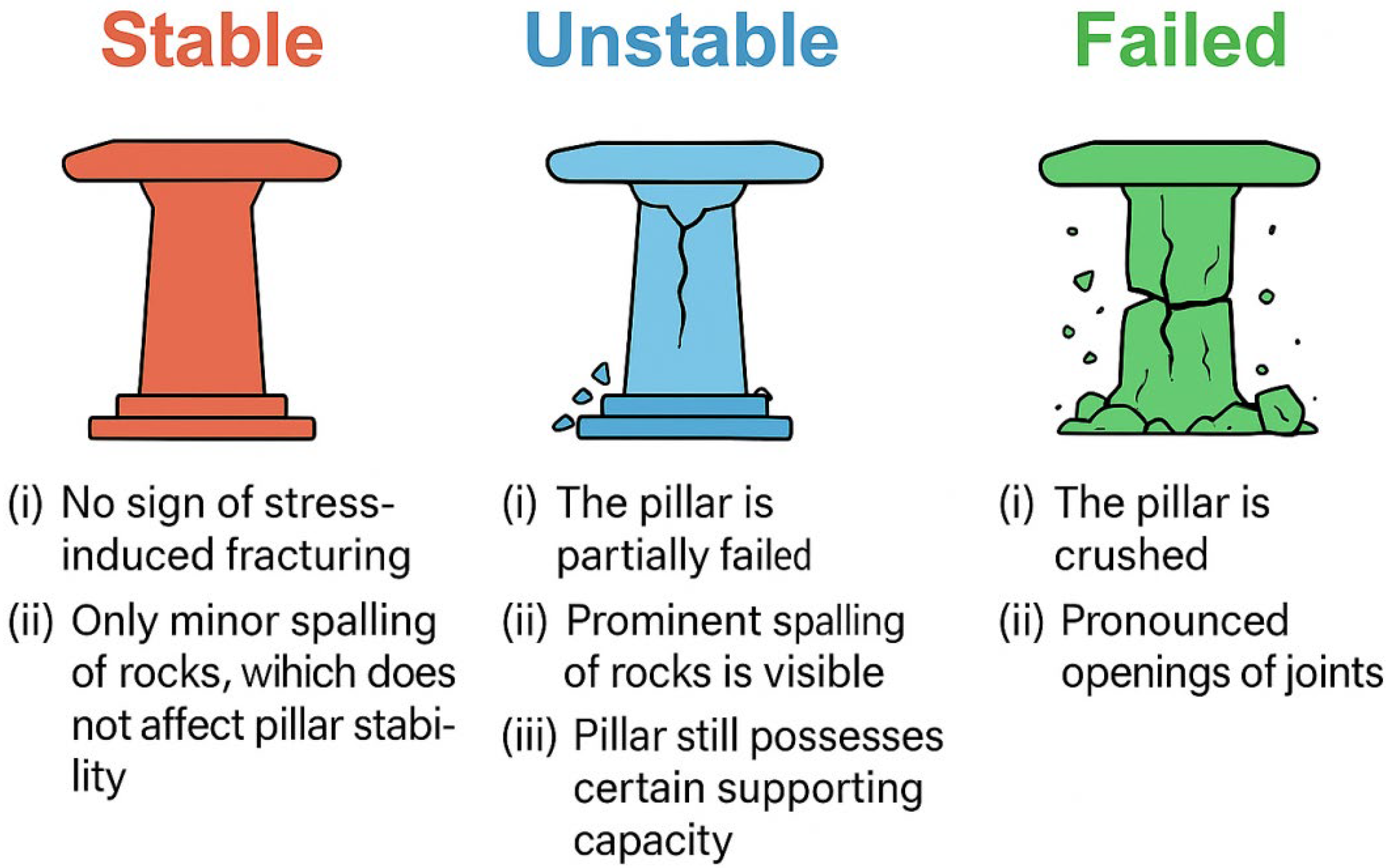
The dataset used in this study was compiled from seven representative hard-rock mines reported in previous research, covering a wide range of lithologies, stress environments, and mining methods, with a total of 241 pillar cases. Specifically, the data were collected from the Elliot Lake uranium mine [31] (M1), the Selebi-Phikwe mine [32] (M2), an open stope mine [33] (M3), the Zinkgruvan Zn mine [34] (M4), Westmin Resources Ltd.’s H-W mine [35] (M5), a marble mine [36] (M6), and a stone mine [5] (M7). For each sample, the stability label was determined according to classification criteria established in previous studies based on field observations of pillar deformation characteristics, failure modes, and stress redistribution patterns [37,38]. The hard-rock pillar stability was categorized into three classes of Stable, Unstable, and Failed (as shown in Figure 1), corresponding to labels 1, 2, and 3 respectively. As illustrated, stable pillars maintain intact geometry with only minor spalling and no visible joint opening or stress-induced fracturing; Unstable pillars exhibit prominent spalling, cracking, and local deformation but retain partial load-bearing capacity; while Failed pillars undergo severe fragmentation and collapse, often accompanied by large block falls and joint separations greater than 10 mm.

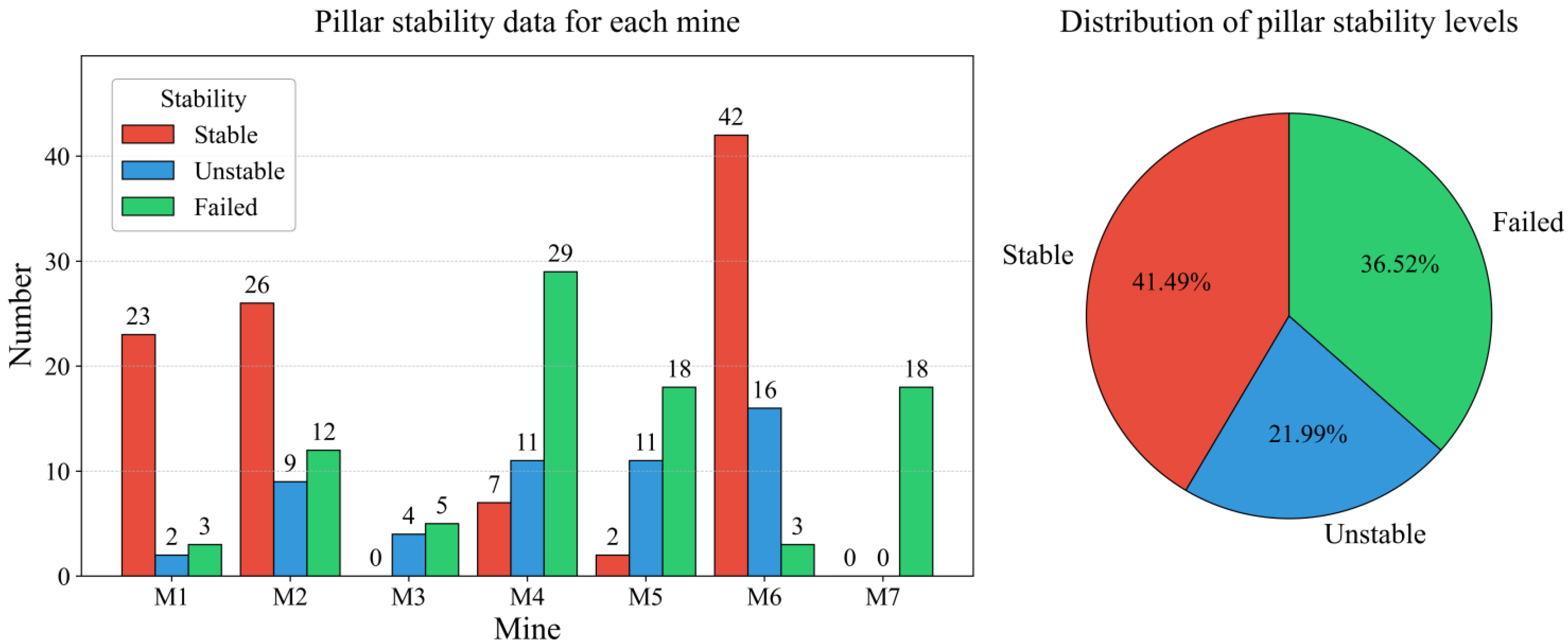
The statistical characteristics of pillar stability state across mines and overall dataset are shown in Figure 2. It is shown that the pillar stability data for each mine reveal a markedly unbalanced and distinct distribution across the seven mining sites. Specifically, M1, M2, and M6 have significantly higher numbers of stable samples (23, 26, and 42, respectively) compared to unstable and failed samples. In contrast, M4, M5, and M7 have the highest number of failed samples. Notably, certain stability levels in M3 and M7 contain zero or very few samples, highlighting the irregularity and complexity of the dataset composition. From the overall distribution of pillar stability levels, the dataset displays a pronounced class imbalance, with Stable, Unstable, and Failed samples accounting for 41.49%, 21.99%, and 36.52% of the total, respectively. Such imbalance increases the complexity of data-driven modeling and poses challenges to the stability and generalization performance of machine learning algorithms.

To quantitatively describe the mechanical behavior of hard-rock pillars, six representative parameters were selected as input features for model development: F1—pillar width (w), F2—pillar height (h), F3—width-to-height ratio, F4—uniaxial compressive strength of rock (UCS), F5—average pillar stress (Ps), and F6—Stress-to-UCS ratio. These parameters comprehensively characterize the geometric configuration, material properties, and stress conditions of pillars, and have been widely adopted in previous pillar stability studies [36,39].

The statistical characteristics of the input features also provide valuable insights into the data structure. These continuous variables vary widely in scale and distribution, which may impact model training and normalization strategies. The descriptive statistics of input features for the pillar stability dataset are summarized in

Table 1. The statistical analysis of the pillar stability data.

Statistical Indicators	F1: w (m)	F2: h (m)	F3: w/h	F4: UCS (MPa)	F5: Ps (MPa)	F6: Ps/UCS
Min value	1.90	2.40	0.21	7.60	0.14	0.00
Max value	45.00	61.00	4.50	316.00	215.00	23.89
Mean value	11.34	12.40	1.17	128.64	53.69	1.23
Standard deviation	7.76	11.29	0.60	70.83	46.30	3.67
25th percentiles	5.30	3.80	0.77	90.00	16.67	0.13
50th percentiles	9.00	7.30	1.00	104.00	48.00	0.33
75th percentiles	16.00	17.00	1.42	176.00	72.40	0.54
Skew	1.22	1.73	1.90	0.51	1.30	4.47
Kurtosis	4.44	6.11	9.03	2.60	4.98	23.59

. The minimum and maximum values indicate the observed range for each variable. The mean and percentile values (25th, 50th, and 75th) reflect the central tendency and distribution spread. The standard deviation measures the variability within each feature. Skewness and kurtosis are also reported to characterize the asymmetry and peakedness of the data distributions, providing further insight into the data structure.

2.2. Data Analysis

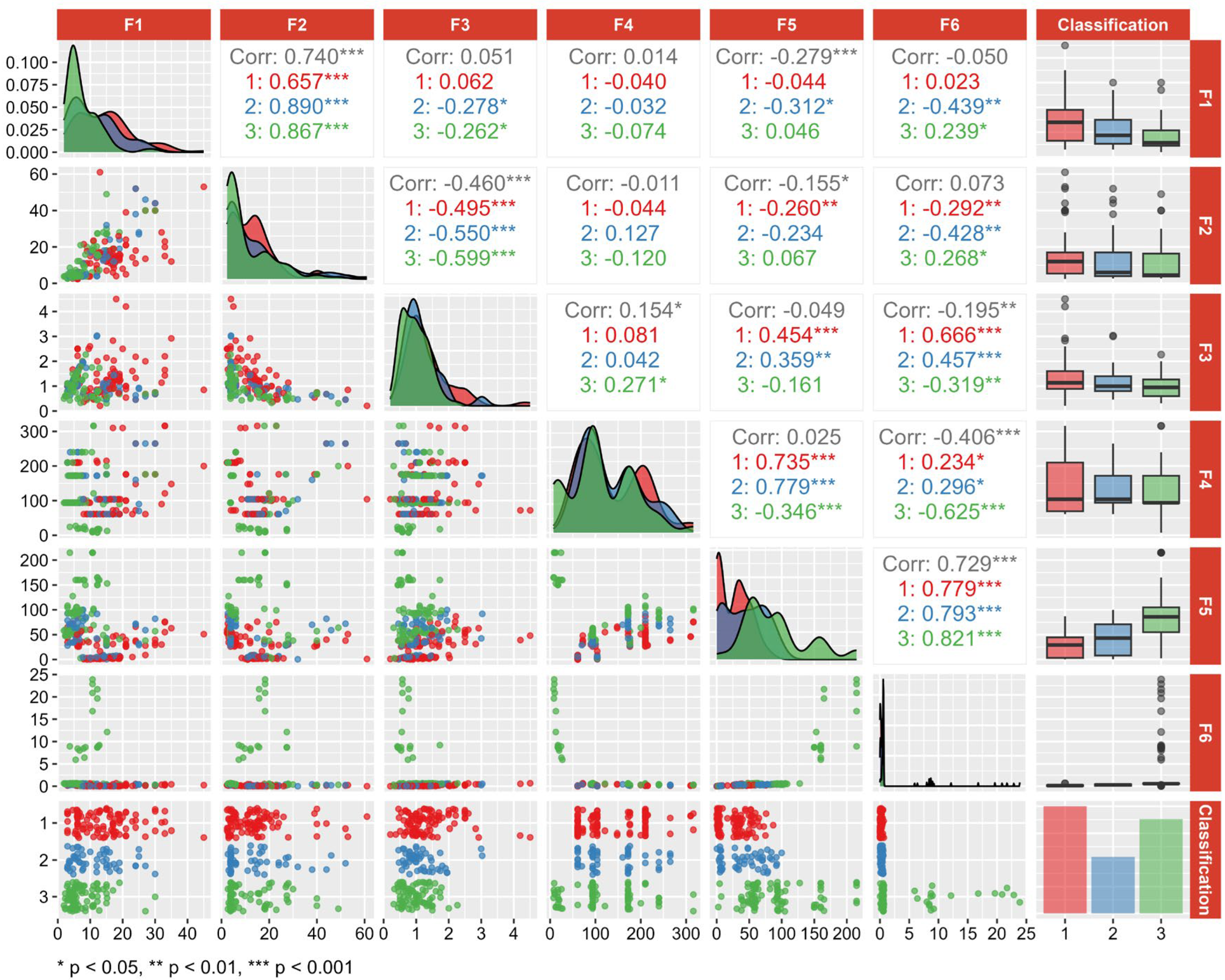
The pairwise correlation matrix and class-wise distributions of the six input features are shown in Figure 3. It illustrates the interrelationships among variables and their dependence on pillar stability categories. In detail, the diagonal panels display the probability density plots of individual features, reflecting their statistical characteristics. The off-diagonal panels represent the pairwise relationships under different stability conditions: the lower triangle shows scatterplots between feature pairs, while the upper triangle presents Pearson correlation coefficients. The rightmost column of boxplots and the bottom row of strip plots summarize how each feature varies across the three pillar stability classes, revealing overall distributional patterns.

The probability density plots and boxplots indicate that the distributions of pillar stability categories exhibit substantial overlap across individual features. This pattern suggests the difficulty to accurately predict pillar stability based solely on one or two variables. The bottom row of categorical scatterplots shows that most feature values are concentrated in the lower range, though a noticeable number of outliers are present. In particular, for feature F6, the majority of samples are concentrated between 0 and 2, but the Failed category (class 3) contains a notable number of outliers distributed in the 5–25 range. The pairwise scatterplots and Pearson correlation coefficients further reveal linear relationships among features. F1 and F2 have a strong positive correlation (r = 0.740), as do F5 and F6 (r = 0.729). Conversely, F2 and F3 exhibit moderate negative correlation (r = −0.460), as do F4 and F6 (r = −0.406). However, most feature pairs display only weak or moderate correlations, indicating a relatively high degree of independence among variables. Therefore, to fully capture the underlying data characteristics, all six features were retained as input variables in the subsequent modeling process.

3. Methodologies

3.1. Super Learner (SL)

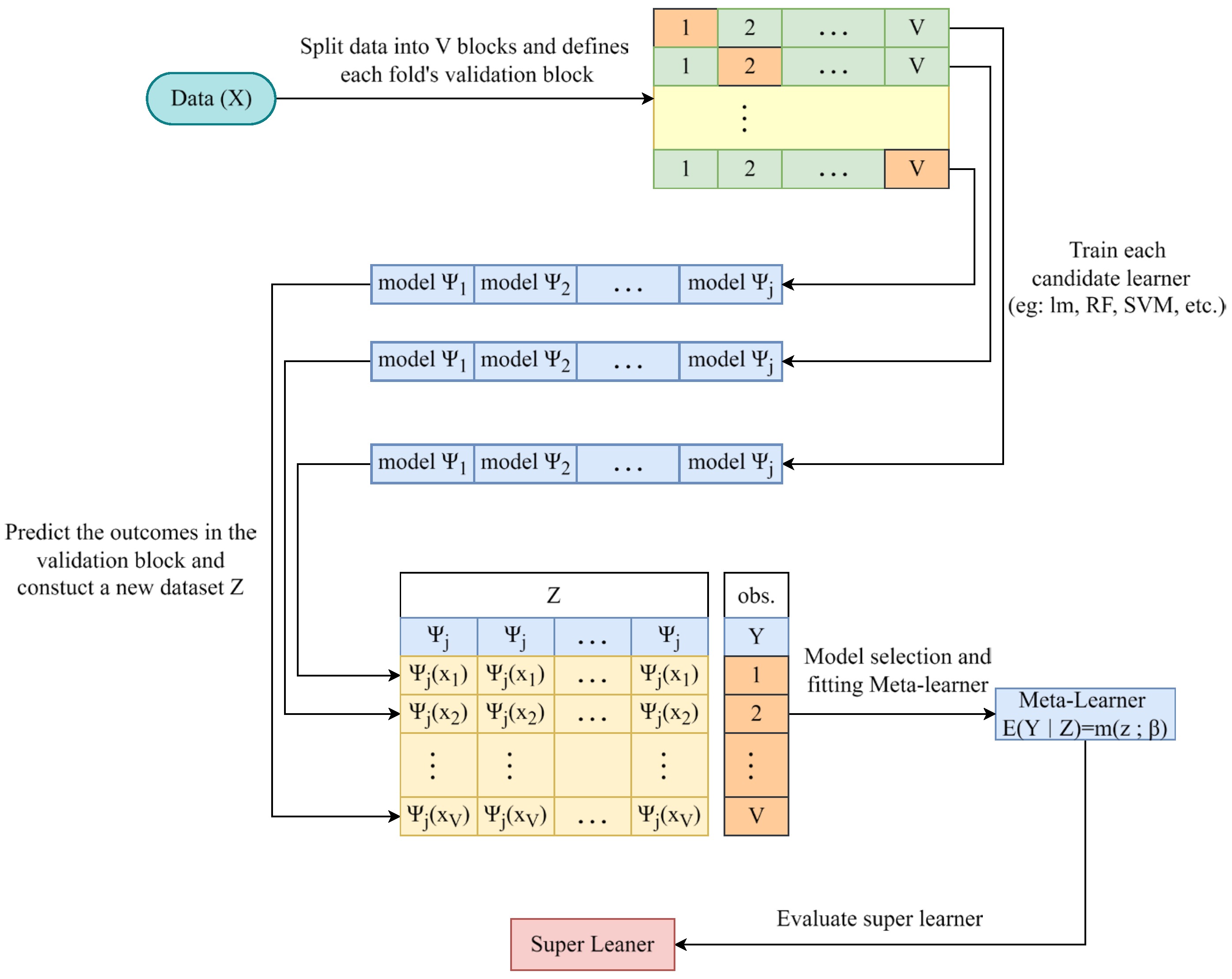
The Super Learner (SL) is an ensemble learning algorithm proposed by van der Laan et al. [40,41]. It aims to construct an optimal predictive model by combining a set of base learners through cross-validation and loss-based optimization. Instead of choosing a single best algorithm, SL leverages the strengths of multiple candidate models and asymptotically performs as well as the best convex combination of them. As shown in Figure 4, the Super Learner framework consists of the following four stages:

(1)

Define a library of prediction algorithms

Define a set of $J$ candidate learners $L=\left\{{\Psi }_1,{\Psi }_2,\dots ,{\Psi }_j\right\}$, each of which produces a prediction based on input features $X$. These may include regression, classification, or nonparametric machine learning methods.

(2)

V-Fold Cross-Validation

Divide the data into V equal-sized folds. For each learner ${\Psi }_j$, fit the algorithm on V-1 folds and generate predictions on the remaining fold. This is repeated across all folds to generate cross-validated predictions for each algorithm.

(3)

Fit a meta-learner to combine predictions

Use the cross-validated predictions to construct a new dataset $Z$, where each column corresponds to one candidate learner’s predictions. A meta-learner is then fitted by regressing the observed outcomes $Y$ on $Z$, optimizing weights $\beta$ for a convex combination of the learners:

$${\widehat{\Psi }}_{SL}(X)={\displaystyle \sum _{j=1}^J{\beta }_j^{*}}{\Psi }_j(X).$$

(1)

(4)

Final prediction

Each candidate learner is retrained on the full dataset, and the final prediction is generated using the optimized weighted combination.

This framework enables the integration of heterogeneous learning algorithms in a theoretically optimal manner, effectively reducing variance and improving generalization performance.

3.2. Osprey Optimization Algorithm (OOA)

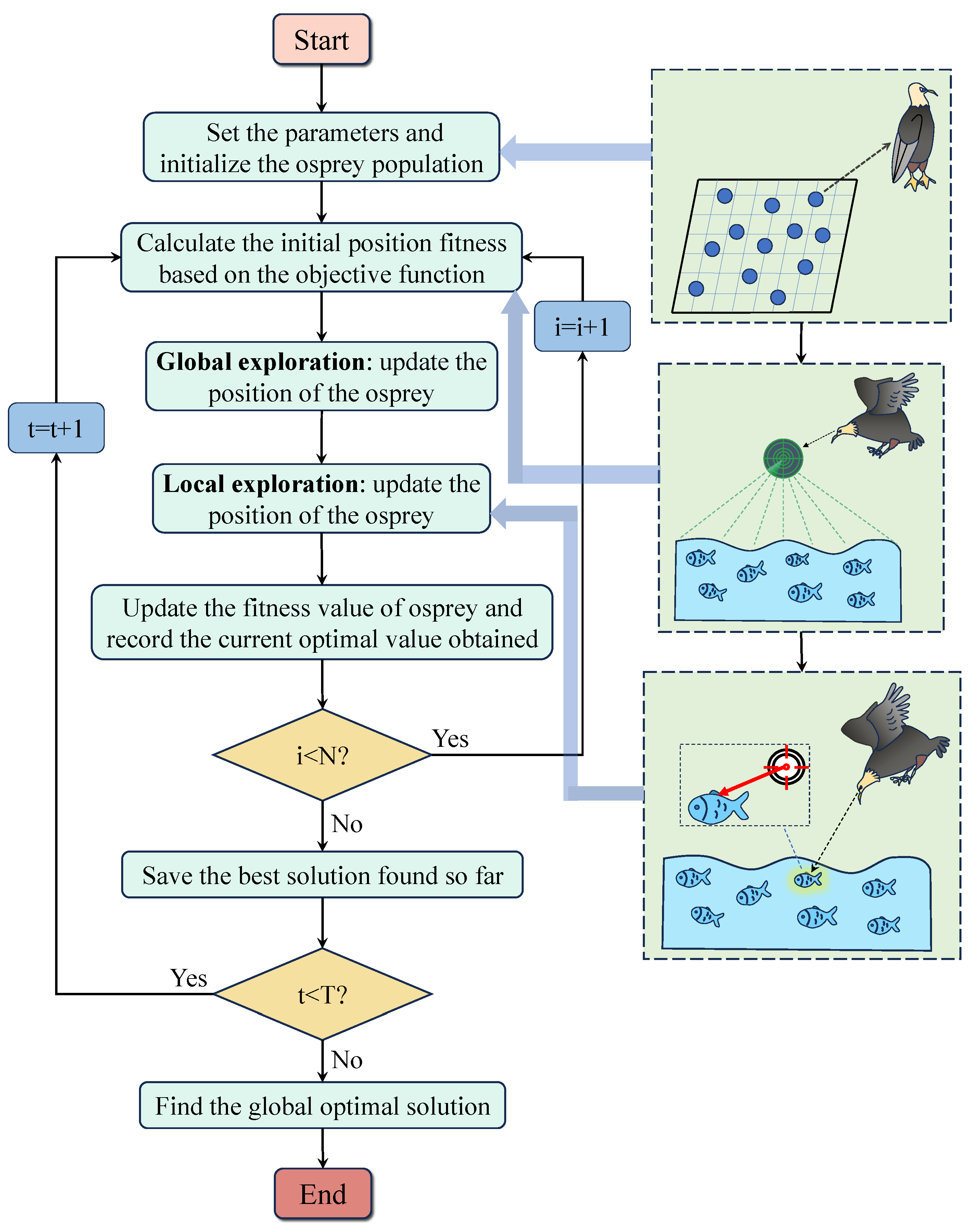
The OOA is a novel biological metaheuristic optimization algorithm proposed by Dehghani and Trojovsky [42]. The flow chart is shown in Figure 5. OOA simulates the predation behavior of osprey in nature. Based on the simulation of the osprey hunting process, a mathematical model of the two stages of exploration and development of osprey is established. It has the advantages of strong global search ability, rapid convergence speed, and small sensitivity to the initial value. The specific steps of OOA are as follows:

(1)

Osprey population initialization

The OOA is a population-centric approach designed to solve complex problems. Within this framework, each individual within the population symbolizes a potential solution to the problem at hand. The ospreys collectively constitute the population of the OOA, represented by a matrix for mathematical modeling. This matrix facilitates the assessment of the population members’ searchability within the problem-solving space, enabling iterative refinement of solutions. Initially, the positions of the ospreys within the search space are randomized, ensuring a broad exploration of potential solutions. As the iterations progress, each osprey functions akin to a sensor node, providing crucial location information. This collaborative effort aids in the gradual convergence of the current problem towards an optimal solution. The matrix representing the initial osprey population can be expressed as follows:

$$X={\left[\begin{array}{c}{X}_1\\ ⋮\\ X_2\\ ⋮\\ X_3\end{array}\right]}_{N\times m}={\left[\begin{array}{ccccc}{x}_{1,1}& \dots & x_{1,j}& \dots & x_{1,m}\\ ⋮& \ddots & ⋮& ⋰& ⋮\\ x_{i,1}& \dots & x_{i,j}& \dots & x_{i,m}\\ ⋮& ⋰& ⋮& \ddots & ⋮\\ x_{N,1}& \dots & x_{N,j}& \dots & x_{N,m}\end{array}\right]}_{N\times m},$$

(2)

$$x_{i,j}=l{b}_j+r_{i,j}\cdot \left(u{b}_j-l{b}_j\right),i=1,2,\dots ,N,j=1,2,\dots ,m,$$

(3)

where $X$ represents the population matrix of ospreys’ locations; $X_i$ is the $ith$ osprey (a candidate solution); $x_{i,j}$ represents its $jth$ dimension (problem variable); $N$ denotes the number of ospreys; $m$ stands for the number of problem variables; $r_{i,j}$ is a random number within the interval [0,1]; $l{b}_j$ and $u{b}_j$ corresponds to the lower bound and upper bound of the $jth$ problem variable, respectively.

Since each osprey is a candidate solution to the problem, the objective function value of the problem can be expressed as:

$$F={\left[\begin{array}{c}{F}_1\\ F_2\\ F_3\\ ⋮\\ F_N\end{array}\right]}_{N\times 1},$$

(4)

where $F$ is the vector of the objective function values; $F_i$ indicates the objective function value of $X_i$.

(2)

Positioning and fishing (global exploration)

The optimal solution within the OOA is attained by simulating the osprey’s search and observation processes. Once the osprey locates its prey, it swiftly attacks and captures the fish. This mimicry not only enhances the algorithm’s exploration capabilities, but also enables it to discern optimal regions more effectively and avoid local minima. The optimal solution is embodied in the position of the fish shoal. It can be represented by the osprey’s location in the search space that yields the highest objective function value. In essence, the fish shoal position corresponds to the osprey’s location yielding the peak performance in terms of the objective function. The fish shoal position of the $ith$ osprey is:

$$P_i=\left\{X_k|k\in \left\{1,2,3,\dots ,N\right\}\cap F_k<F_i\right\}\cup \left\{X_{best}\right\},$$

(5)

where $P_i$ is the set of shoal positions for the $ith$ osprey; $X_{best}$ is the value of $X_i$ corresponds to the optimal $F_i$.

The osprey randomly selects the position of a fish and attacks. By simulating the movement of the osprey to the fish, the new position of the osprey is determined by the following formulas:

$$x_{i,j}^1=x_{i,j}+r_{i,j}\left(P_{i,j}^S-I_{i,j}\cdot x_{i,j}\right),$$

(6)

$$x_{i,j}^1=\left\{\begin{array}{c}{x}_{i,j}^1,l{b}_j\le x_{i,j}^1\le u{b}_j\\ l{b}_j, x_{i,j}^1<l{b}_j\\ u{b}_j,x_{i,j}^1>u{b}_j\end{array}\right.,$$

(7)

where $x_{i,j}^1$ is the new position of the $ith$ osprey in the $jth$ problem variable; $P_{i,j}^S$ the position of the fish selected by the $ith$ osprey in the $jth$ problem variable; $I_{i,j}$ is the random number in the set [1,2].

The position of the osprey is updated if the objective function value at the new position is improved. The new location of the updated osprey is:

$$X_i=\left\{\begin{array}{c}{X}_i^1,F_i^1<F_i\\ X_i,F_i^1\ge F_i\end{array}\right.,$$

(8)

where $X_i^1$ is the new position of the $ith$ osprey; $F_i^1$ is the objective function value of $X_i^1$.

(3)

Bring the fish to the right position (local exploration)

After completing the pre-hunt, the osprey takes the fish to where it believes it is safe to eat. This process will only fine-tune the osprey’s position within the search area and enhance the local search capability of OOA. At this stage, the position of the osprey will be updated again. Similar to the global exploration phase, this phase also requires a boundary processing operation, such as the following formulas:

$$x_{i,j}^2=x_{i,j}+{\displaystyle \frac{l{b}_j+r_{i,j}\cdot \left(u{b}_j-l{b}_j\right)}{t}}, i=1,2,\dots ,N; j=1,2,\dots ,m; t=1,2,\dots ,T,$$

(9)

$$x_{i,j}^2=\left\{\begin{array}{c}{x}_{i,j}^2,l{b}_j\le x_{i,j}^2\le u{b}_j\\ l{b}_j, x_{i,j}^2<l{b}_j\\ u{b}_j,x_{i,j}^2>u{b}_j\end{array}\right.,$$

(10)

where $x_{i,j}^2$ is its $jth$ dimension; $r_{i,j}$ is a random number belonging to [0,1]; $t$ is the current number of iterations of the algorithm; $T$ is the maximum number of iterations.

If the position updated according to Equations (9) and (10) has a better fitness value, the new position will replace the previous position. This process is like the global exploration phase. The updated position of the osprey in this phase can be determined according to the following formula:

$$X_i=\left\{\begin{array}{c}{X}_i^2,F_i^2<F_i^1\\ X_i,F_i^2\ge F_i^1\end{array}\right.,$$

(11)

where $F_i^2$ represents the fitness value of the location $X_i^2$, $X_i$ represents the osprey’s position after the second stage.

After the above two stages, the OOA will update the positions of all ospreys and iterate the population. This process will continue until the optimal solution to the problem is found or the maximum number of iterations is reached.

3.3. Borderline-SMOTE (BSMOTE)

Borderline-SMOTE is an enhanced oversampling technique derived from the original Synthetic Minority Over-sampling Technique (SMOTE). It is designed to address the problem of class imbalance in classification tasks [43]. The standard SMOTE generates synthetic samples randomly along the line segments connecting minority class instances and their nearest neighbors. Borderline-SMOTE, on the other hand, selectively generates new samples near the decision boundary, where misclassification is most likely to occur. The key idea behind Borderline-SMOTE is to focus on “dangerous” minority instances—those surrounded by a significant number of majority class neighbors. These borderline points are more likely to be misclassified and thus are critical for improving classification performance. The algorithm proceeds as follows:

(1)

For each sample in the minority class, compute its $\mathrm{k}$ nearest neighbors;

(2)

Identify “dangerous” samples whose majority class neighbors exceed a defined threshold;

(3)

Generate synthetic samples only for these dangerous instances by interpolating with their minority neighbors.

By concentrating on the difficult-to-classify regions, Borderline-SMOTE helps enhance the classifier’s decision boundary and reduces the risk of overfitting caused by redundant or irrelevant synthetic samples. In this study, Borderline-SMOTE is applied during the model training phase to rebalance the dataset and improve the generalization ability of the Super Learner ensemble.

3.4. Proposed BSMOTE-OOA-SL Framework

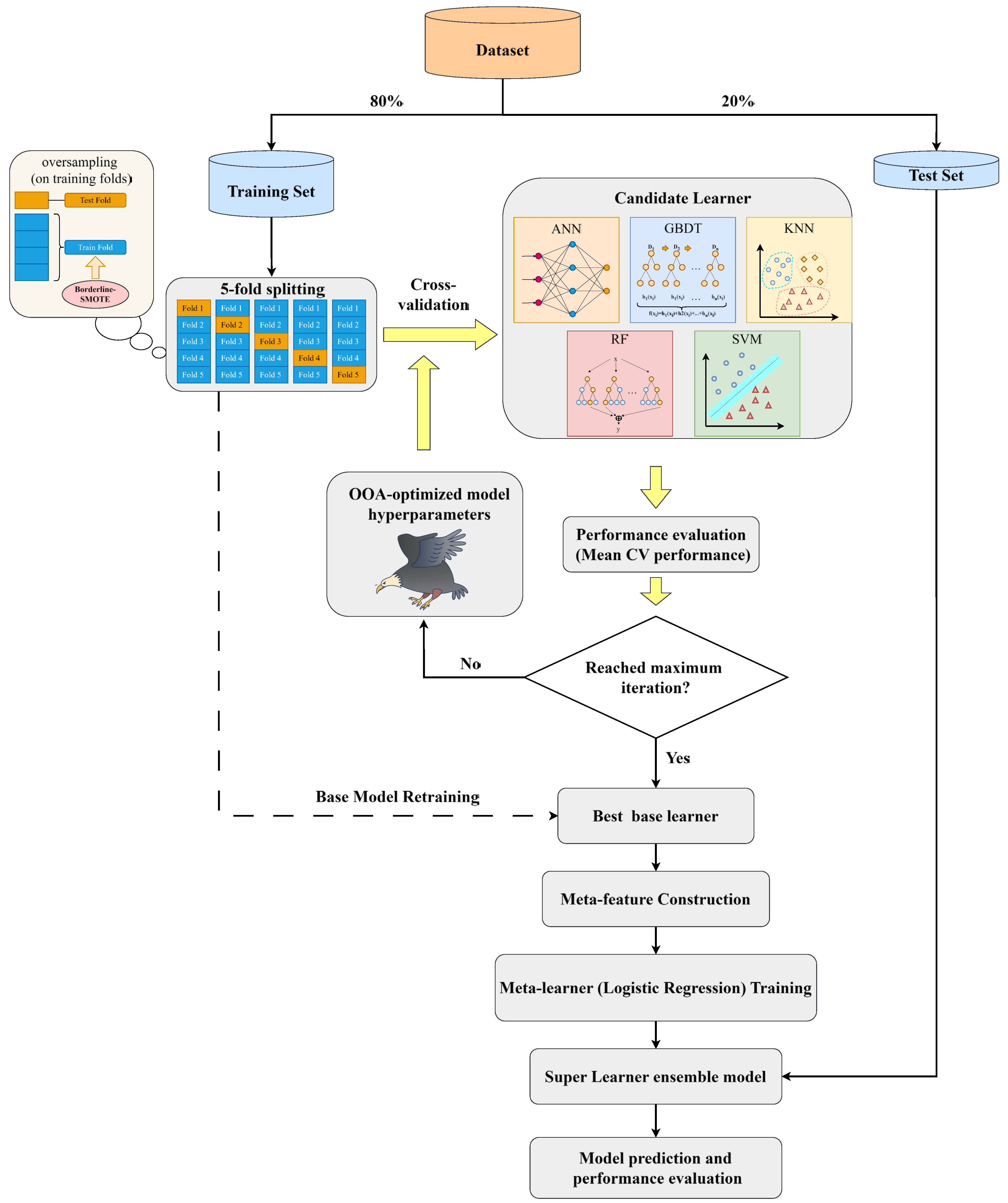
The proposed BSMOTE-OOA-SL Strategy is an integrated learning framework, as shown in Figure 6. BSMOTE is used to address class imbalance problem in the dataset, and the OOA is applied to optimize the selected base learners in the framework. Different machine learning algorithms are integrated through the Super Learner (SL) method to build a stable and high-performance pillar stability prediction model. The details of model development are as follows:

(1)

Base learner selection

As a stacking ensemble strategy, the performance of the Super Learner model depends on the diversity and quality of the base learners [44]. By integrating base learners with different characteristics, it is possible to maximize the recognition of useful information in the data and fully leverage the complementary strengths of each base learner. Thereby, the overfitting risks associated with relying on a single algorithm can be reduced. In the proposed framework, the following five base learners with complementary strengths were selected:

Artificial Neural Network (ANN): Capable of effectively learning complex non-linear relationships in high-dimensional data, especially suitable for tasks with intricate feature interactions.

Gradient Boosting Decision Trees (GBDT): Known for its high accuracy in both regression and classification tasks, GBDT can iteratively improve prediction performance by correcting the errors made by previous models.

K-Nearest Neighbors (KNN): A non-parametric method suitable for tasks with uncertain data distributions, especially effective when class boundaries are irregular.

Random Forest (RF): An ensemble method that reduces variance by aggregating multiple decision trees, suitable for high-dimensional and noisy datasets.

Support Vector Machine (SVM): Performs exceptionally well in high-dimensional spaces and is particularly advantageous when the margin of separation between classes is well-defined.

(2)

Borderline-SMOTE resampling

In the proposed framework, the dataset is divided into training and testing sets in an 8:2 ratio, with the training set used for model optimization and training, and the testing set reserved solely for evaluation. The training set is further divided into five folds in equal proportions, with one fold used as the validation fold and the remaining four folds as train folds. The five-fold split of the training set is used for two purposes: (1) cross-validation during the optimization of the base learners, and (2) training the optimized base learners and generating meta-features. As mentioned in Section 2, the dataset exhibits significant class imbalance. To mitigate its impact, oversampling is applied to balance the minority class. In this study, Borderline-SMOTE is applied only to the “training folds” of the training set, rather than oversampling the entire training dataset. This approach ensures that during cross-validation and meta-feature generation, the validation fold is not influenced by synthetic samples, thus preventing data leakage and avoiding bias in model performance and calibration [45,46].

(3)

Hyperparameter optimization based on OOA

In the proposed strategy, the hyperparameters of each base learner are optimized independently using the Osprey Optimization Algorithm (OOA). During the optimization process, 5-fold cross-validation is employed to evaluate each set of candidate hyperparameter configurations. This cross-validation process is embedded within the OOA framework to avoid overfitting and ensure that the selected hyperparameters generalize well to unseen data. The optimization objective is logarithmic loss, which is particularly suitable for evaluating the performance of probabilistic classifiers. After optimizing the hyperparameters with OOA, each model is retrained on the complete resampled training set to ensure that the final model is trained using the best hyperparameter configuration.

(4)

Super Learner stacking framework

Once the base learners have been optimized, their prediction results are combined using the Super Learner stacking method. In the two-layer stacking structure, each base learner generates probability predictions for the target class, and these predictions serve as features for the meta-learner. The meta-learner is a logistic regression model, which learns an optimal weighted combination of the probability outputs from base learners under its standard likelihood-based objective. The final Super Learner model is trained on the complete resampled training set, ensuring that the ensemble process fully utilizes the balanced data optimized by Borderline-SMOTE and the optimization results of each base learner, thereby enhancing the overall accuracy and robustness of the predictions.

3.5. Evaluation Indicators

As discussed in Section 2, the hard-rock pillar stability dataset consists of three classes: Stable, Unstable, and Failed, which constitutes a multi-class classification problem. The objective of the proposed machine learning framework is to accurately identify these stability states. Therefore, appropriate evaluation indicators are required to comprehensively assess classification performance, particularly under conditions of class imbalance [47]. In this study, model performance is evaluated using Accuracy (ACC), Macro-Precision, Macro-Recall, and Macro-F1, together with the Receiver Operating Characteristic (ROC) curve and the Area Under the Curve (AUC). These metrics are widely adopted in multi-class classification tasks and have been proven effective in previous pillar stability and engineering-related studies.

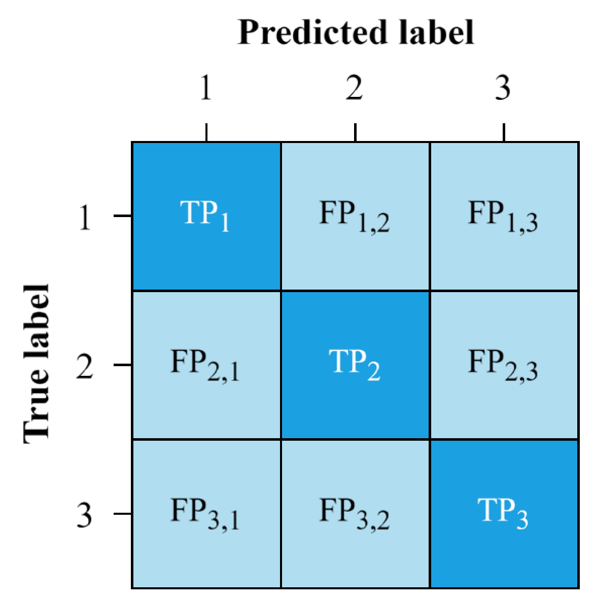
Accuracy and the class-wise Precision, Recall, and F1 Score can be computed using the confusion matrix. For the mineral pillar stability classification problem presented in this paper, the confusion matrix is derived from the statistical results after the model’s predictions, as shown in Figure 7. In this matrix, $T{P}_c$ refers to the number of samples that actually belong to class $c$ and are correctly predicted as class $c$, while $F{P}_{i,j}$ represents the number of samples that actually belong to class $i$ but are incorrectly predicted as class $j$. The following formulas can be used to compute Accuracy, Precision, Recall, and F1 Score:

$$Accurac{y}_c=({\displaystyle \frac{1}{D}}{\displaystyle \sum _{c=1}^{3}T{P}_c})\times 100\%,$$

(12)

$$Precisio{n}_c=({\displaystyle \frac{T{P}_c}{T{P}_c+F{P}_c}})\times 100\%,$$

(13)

$$Recal{l}_c=({\displaystyle \frac{T{P}_c}{T{P}_c+F{N}_c}})\times 100\%,$$

(14)

$$F{1}_c=({\displaystyle \frac{2\cdot Precisio{n}_c\cdot Recal{l}_c}{Precisio{n}_c+Recal{l}_c}})\times 100\%,$$

(15)

where $c$ represents a specific class; $D$ is the total number of samples; $T{P}_c$ is the number of samples that actually belong to class $c$ and are correctly predicted as class $c$; $F{P}_c$ is the number of samples that do not belong to class $c$ but are incorrectly predicted as class $c$; and $F{N}_c$ is the number of samples that actually belong to class $c$ but are incorrectly predicted as another class.

To account for class imbalance and to provide an unbiased evaluation across all classes, macro-averaged metrics are adopted in this study. Macro-Precision, Macro-Recall, and Macro-F1 are calculated as the arithmetic mean of the corresponding class-wise metrics:

$$Macro\_Precisio{n}_c={\displaystyle \frac{1}{K}}{\displaystyle \sum _{c=1}^{K}Precisio{n}_c}\times 100\%,$$

(16)

$$Macro\_Recal{l}_c={\displaystyle \frac{1}{K}}{\displaystyle \sum _{c=1}^{K}Recal{l}_c}\times 100\%,$$

(17)

$$Macro\_F{1}_c={\displaystyle \frac{1}{K}}{\displaystyle \sum _{c=1}^{K}F{1}_c}\times 100\%,$$

(18)

where $K$ denotes the number of classes (in this study, $K=3$).

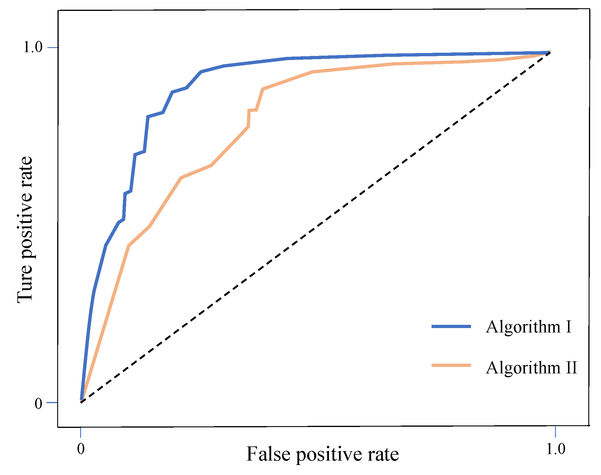
The ROC curve is widely utilized as a tool for evaluating the performance of classification models, as depicted in Figure 8. It demonstrates how the models’ performance varies across different thresholds. The closer the ROC curve approaches the upper left corner, the more superior the models’ performance. The performance of these models can be quantitatively assessed by calculating the area under the curve (AUC). The value of AUC ranges from 0 to 1, and the closer the AUC value is to 1, the better the performance of the model.

4. Results and Analysis

4.1. Statistical Performance Analysis

To examine the statistical robustness of the proposed framework, the performance of all base learners and the BSMOTE-OOA-SL model was evaluated using 20 independent random train–test splits generated with different random seeds. The same experimental protocol was applied in all runs. In this stage, a relatively lightweight OOA configuration was adopted, as the focus is on statistical stability rather than achieving peak performance.

Table 2. Statistical performance of base learners and BSMOTE-OOA-SL over 20 random seeds.

Model	Accuracy (Mean ± Std)	Macro-Pr (Mean ± Std)	Macro-Re (Mean ± Std)	Macro-F1 (Mean ± Std)
ANN	0.742 ± 0.101	0.724 ± 0.083	0.713 ± 0.096	0.710 ± 0.098
GBDT	0.774 ± 0.063	0.753 ± 0.069	0.746 ± 0.069	0.743 ± 0.069
KNN	0.676 ± 0.060	0.636 ± 0.066	0.633 ± 0.065	0.630 ± 0.066
RF	0.793 ± 0.062	0.774 ± 0.072	0.760 ± 0.066	0.760 ± 0.068
SVM	0.783 ± 0.050	0.771 ± 0.066	0.754 ± 0.047	0.755 ± 0.050
BSMOTE-OOA-SL	0.830 ± 0.054	0.812 ± 0.069	0.799 ± 0.063	0.800 ± 0.065

Note: The maximum of each metric is highlighted in bold.

reports the mean and standard deviation of Accuracy, Macro-Precision, Macro-Recall, and Macro-F1 across the 20 experiments. The results show that the BSMOTE-OOA-SL model achieves the highest average performance for all evaluation metrics compared with the individual base learners. In addition, its standard deviations are generally smaller, indicating more stable predictive performance under different data partitions.

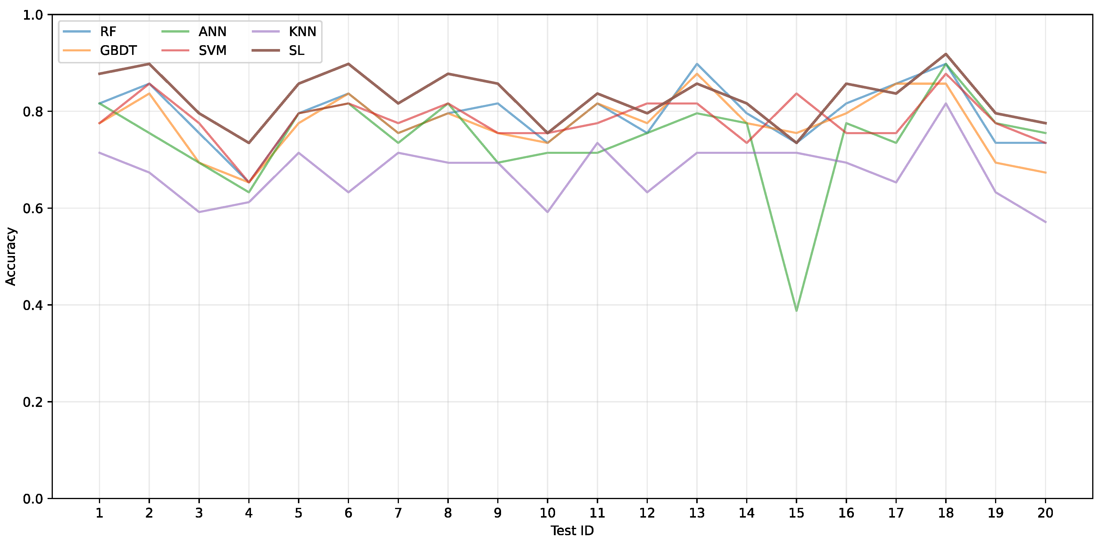
The variation of classification accuracy across the 20 test splits is illustrated in Figure 9. While noticeable fluctuations are observed for several base learners, the BSMOTE-OOA-SL model maintains consistently high accuracy with relatively limited variation. These results indicate that the proposed ensemble framework provides improved robustness against random data partitioning.

4.2. Model Optimization and Prediction Results

Based on the statistical analysis presented in Section 4.1, a fixed and representative data split was selected to further investigate the model optimization process and prediction results. In this stage, a more comprehensive OOA configuration was adopted to allow sufficient exploration of the hyperparameter space and to obtain well-converged optimal solutions. In addition, the predictive performance was analyzed in detail by comparing the proposed BSMOTE-OOA-SL model with individual base learners as well as other competitive machine learning models.

4.2.1. Hyperparameter Optimization Results

Hyperparameter optimization was carried out for each base learner using the Osprey Optimization Algorithm (OOA) based solely on the training data. To ensure adequate exploration of the hyperparameter space and stable convergence behavior, both the population size and the number of iterations of OOA were set to 30.

Table 3. Hyperparameter optimization results for base learners.

Algorithms	Hyperparameters	Population Size	Number of Iterations	Hyperparameter Range	Optimal Values
ANN	hidden_units	30	30	{5, 6, …, 200}	7
	learning_rate	30	30	[10−4, 10−1]	0.002
	activation	30	30	{ReLU, Tanh}	relu
	n_layers	30	30	{1, 2, 3}	1
GBDT	n_estimators	30	30	{50, 51, …, 500}	117
	learning_rate	30	30	[0.01, 0.3]	0.065
	subsample	30	30	[0.5, 1.0]	0.624
	max_depth	30	30	{2, 3, …, 10}	2
KNN	n_neighbors	30	30	{1, 2, …, 100}	23
	p	30	30	[1.0, 3.0]	1
RF	n_estimators	30	30	{10, 11, …, 300}	117
	max_features	30	30	{1, 2, …, 6}	3
	max_depth	30	30	{2, 3, …, 30}	9
	min_samples_split	30	30	{2, 3, …, 20}	4
SVM	C	30	30	[0.1, 200]	109.019
	gamma	30	30	[10−4, 1.0]	0.141
	class_weight_code	30	30	{None, Balanced}	balanced

summarizes the hyperparameter settings adopted in the optimization process, as well as the optimal hyperparameters obtained for the five base learners, including ANN, GBDT, KNN, RF, and SVM.

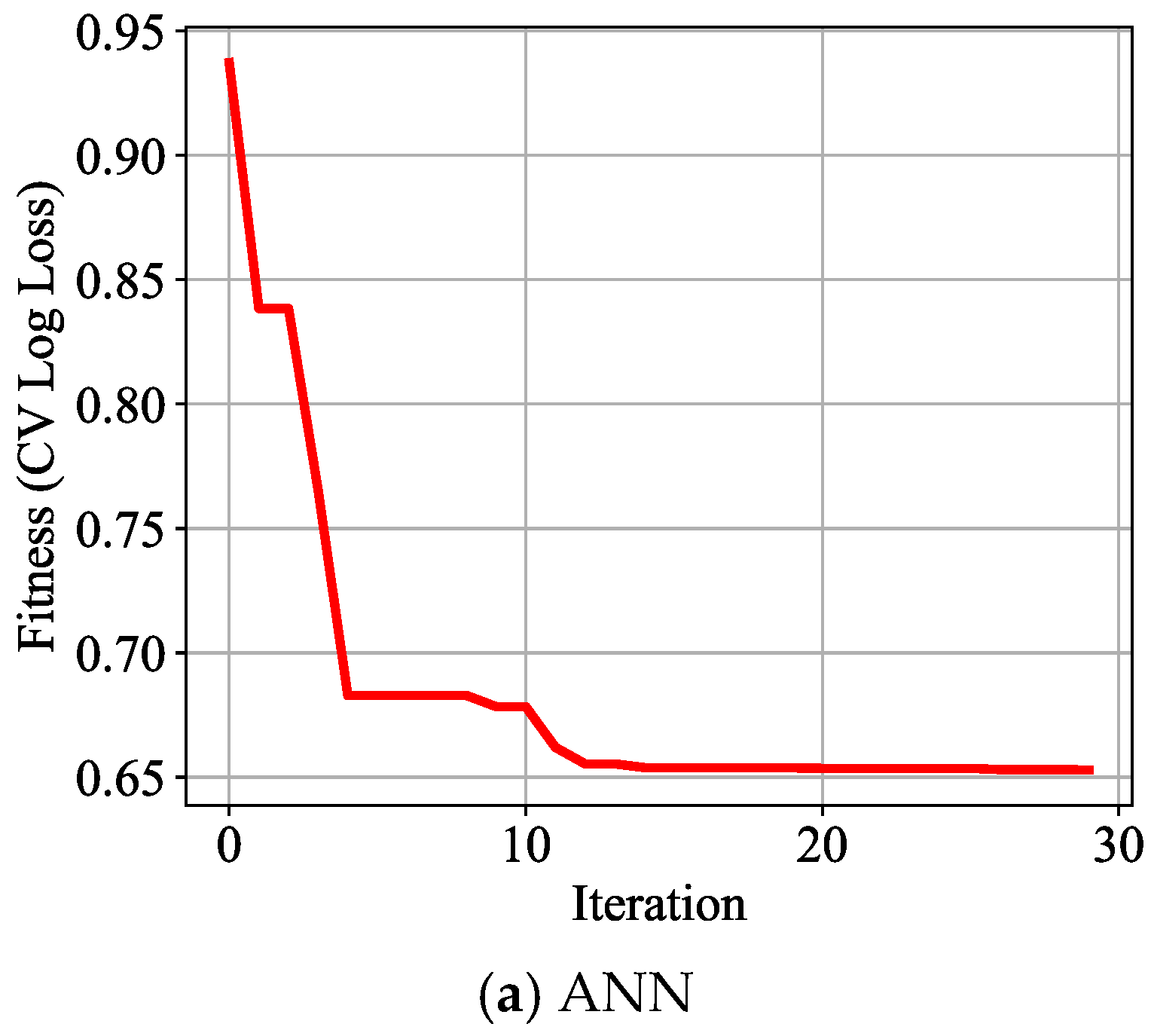
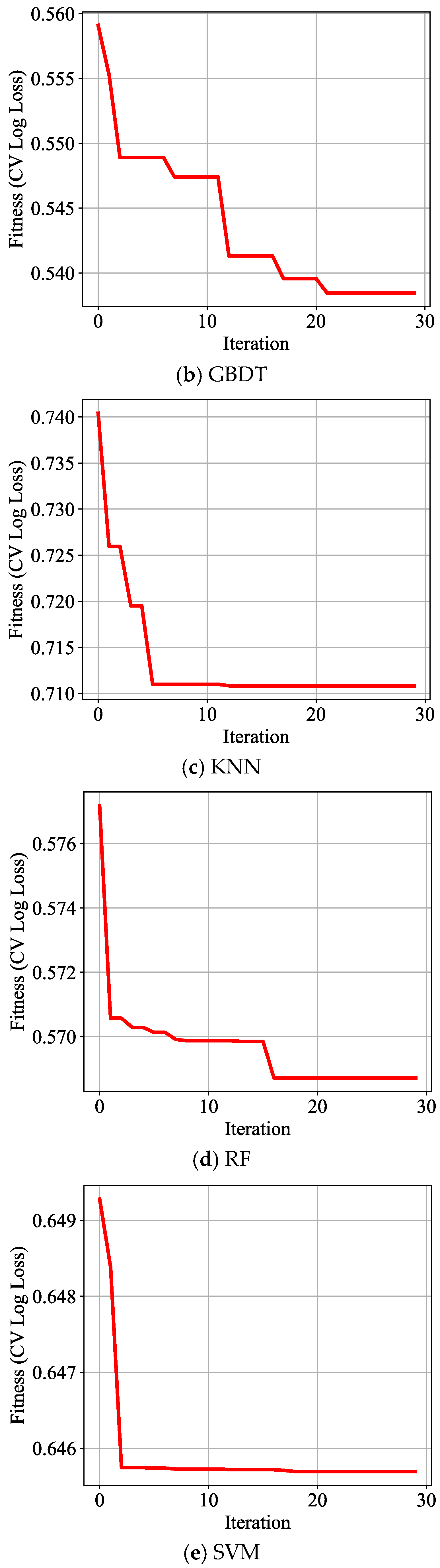
Figure 10 illustrates the variation of the fitness values (cross-validated Log Loss) of each base learner during the hyperparameter tuning process. As the number of iterations increases, the Log Loss values of all base learners gradually decrease and eventually converge, indicating that the models successfully identify favorable hyperparameter combinations through the OOA-based optimization. It is worth noting that all five models converge within 20 iterations, demonstrating that the adopted OOA configuration can efficiently achieve effective hyperparameter optimization.

4.2.2. Model Prediction Results

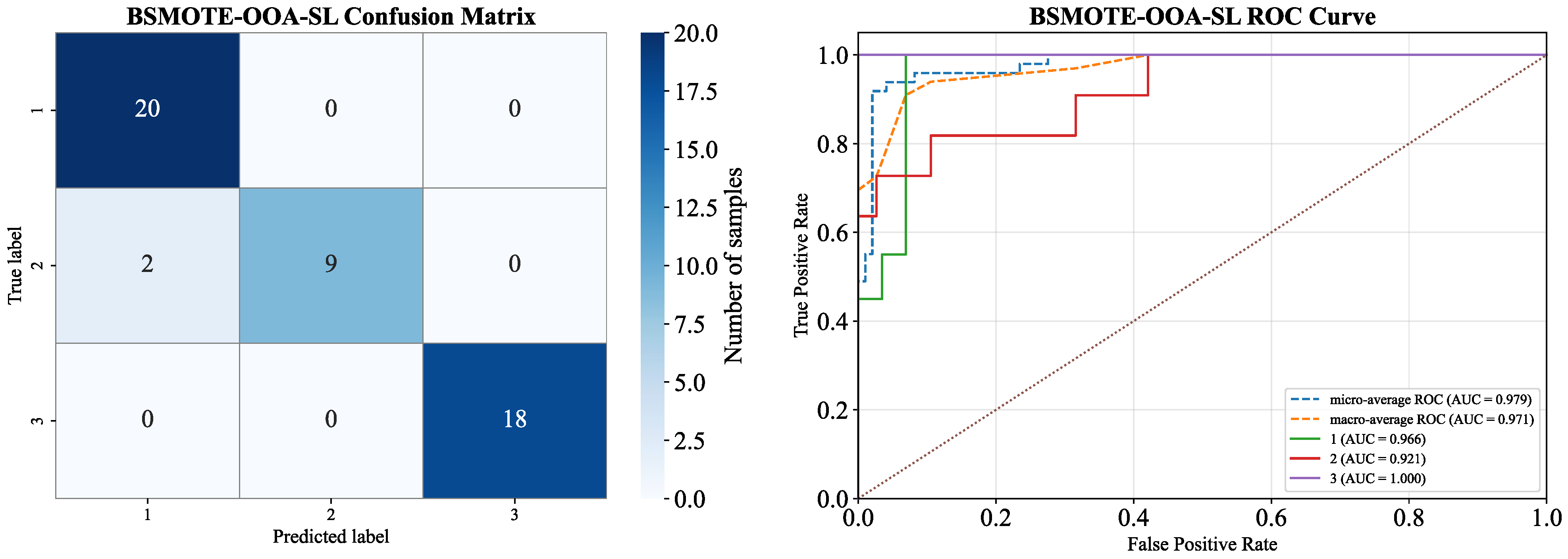
After determining the optimal hyperparameters, the predictive performance of the models was evaluated on the test set. Figure 11 shows the confusion matrix and ROC curves of the BSMOTE-OOA-SL model. The confusion matrix indicates that, among the 49 test samples, only two instances were misclassified, both of which belong to the Unstable class and were predicted as Stable. The ROC curves further illustrate the classification performance for each category. As shown in Figure 10, the AUC values for all three categories exceed 0.9, with the AUC for Category 3 (Failed) reaching 1.0, indicating strong discriminative capability across different classes under the selected data partition.

A quantitative comparison between the proposed BSMOTE-OOA-SL model and other machine learning models is presented in

Table 4. Performance metrics of the BSMOTE-OOA-SL model and other single models in testing.

Model		Accuracy	Precision			Recall			F1-Score
			Stable	Unstable	Failed	Stable	Unstable	Failed	Stable	Unstable	Failed
Compared models	AdaBoost	75.51%	0.708	0.444	1.000	0.850	0.364	0.889	0.773	0.400	0.941
	LGBM	83.67%	0.850	0.636	0.944	0.850	0.636	0.944	0.850	0.636	0.944
	XGBoost	79.59%	0.850	0.600	0.842	0.850	0.546	0.889	0.850	0.571	0.865
	MLP	79.59%	0.778	0.539	1.000	0.700	0.636	1.000	0.737	0.583	1.000
Base learner	ANN	81.63%	0.739	0.625	1.000	0.850	0.455	1.000	0.791	0.526	1.000
	RF	85.71%	0.864	0.700	0.941	0.950	0.636	0.889	0.905	0.667	0.914
	GBDT	83.67%	0.850	0.636	0.944	0.850	0.636	0.944	0.850	0.636	0.944
	SVM	85.71%	0.850	0.700	0.947	0.850	0.636	1.000	0.850	0.667	0.973
	KNN	65.31%	0.750	0.250	0.810	0.600	0.273	0.944	0.667	0.261	0.872
BSMOTE-OOA-SL		95.92%	0.909	1.000	1.000	1.000	0.818	1.000	0.952	0.900	1.000

Note: The maximum of each metric is highlighted in bold.

. The comparison includes both the base learners used in the Super Learner framework (ANN, RF, GBDT, SVM, and KNN) and several competitive high-performance models, such as AdaBoost, LGBM, XGBoost, and MLP. The results show that the BSMOTE-OOA-SL model achieves the highest overall Accuracy, while also outperforming all comparison models in class-wise Precision, Recall, and F1-score across all pillar stability categories. In particular, the overall accuracy reaches 95.92%, demonstrating the effectiveness of the proposed framework under the selected experimental setting.

5. Discussion

5.1. Model Performance Analysis

5.1.1. Impact of Borderline-SMOTE and OOA

The effectiveness of Borderline-SMOTE in addressing class imbalance has been well-documented in the literature. By generating synthetic samples near the decision boundary between classes, it helps improve the classifier’s performance by focusing on the difficult-to-classify borderline samples [48]. Similarly, hyperparameter optimization methods, such as OOA, are widely recognized for their ability to fine-tune individual machine learning models and ensure better performance and generalization [49]. However, in the composite framework proposed in this study, it is essential to evaluate through experiments whether these two techniques effectively contribute to the overall model performance and the extent of their individual impact.

Figure 12 presents a comparison of the full model (utilizing both BSMOTE and OOA) with models that exclude either BSMOTE or OOA. The results show that, compared to the baseline model (without BSMOTE and OOA), using either OOA or BSMOTE alone improves the model’s performance, with BSMOTE providing a greater performance boost than OOA. This is closely related to the high complexity and imbalance of the dataset. By applying BSMOTE oversampling to the dataset, the performance degradation caused by data deficiencies is effectively mitigated. It is noteworthy that the synergistic effect observed when combining OOA and BSMOTE significantly enhanced the model’s performance metrics, with Accuracy, Macro-Precision, Macro-Recall, and Macro-F1 improving by 10.21%, 12.25%, 12.61%, and 12.86%, respectively. This indicates that the BSMOTE oversampling strategy applied to the training set during OOA and cross-validation optimization is effective. In addition to alleviating class imbalance, this strategy helps prevent model over-optimism caused by data leakage, thus improving the model’s generalization and stability when encountering unseen data.

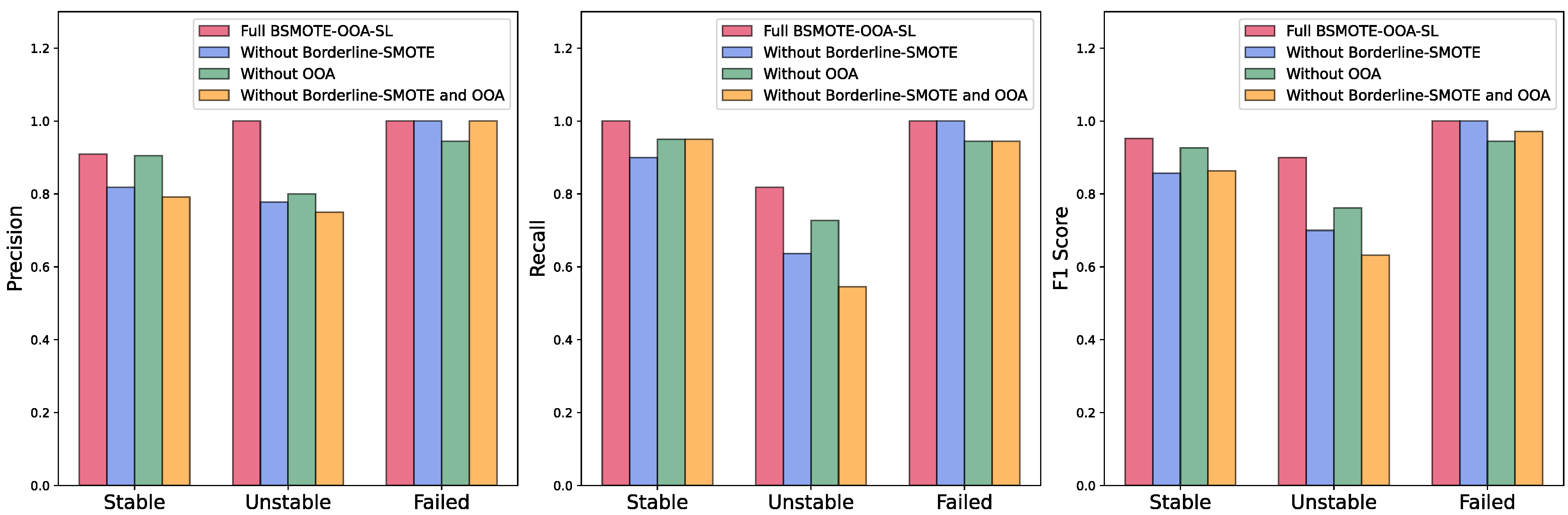
Figure 13 further breaks down the performance of each model across different categories in bar charts. The prediction of the “Unstable” category is clearly more challenging than the other two categories, which is attributed to the differences in mining environment conditions and the way of data collection [24,50]. Nonetheless, the full model (with both OOA and BSMOTE) still outperforms other models, further confirming the effectiveness of these two techniques in enhancing model performance.

5.1.2. Comparison of Super Learner Ensemble Model and Single Models

Ensemble models, in contrast to single models, offer the advantage of combining the predictions of multiple base learners. It thereby harnesses the strengths of each individual model while mitigating their respective weaknesses. This synergy enables ensemble models to achieve performance metrics that surpass those of any single model [51,52]. In this study, the Super Learner framework was employed to integrate five fundamentally distinct machine learning models, aiming to attain the robustness and generalization performance that individual models cannot achieve independently.

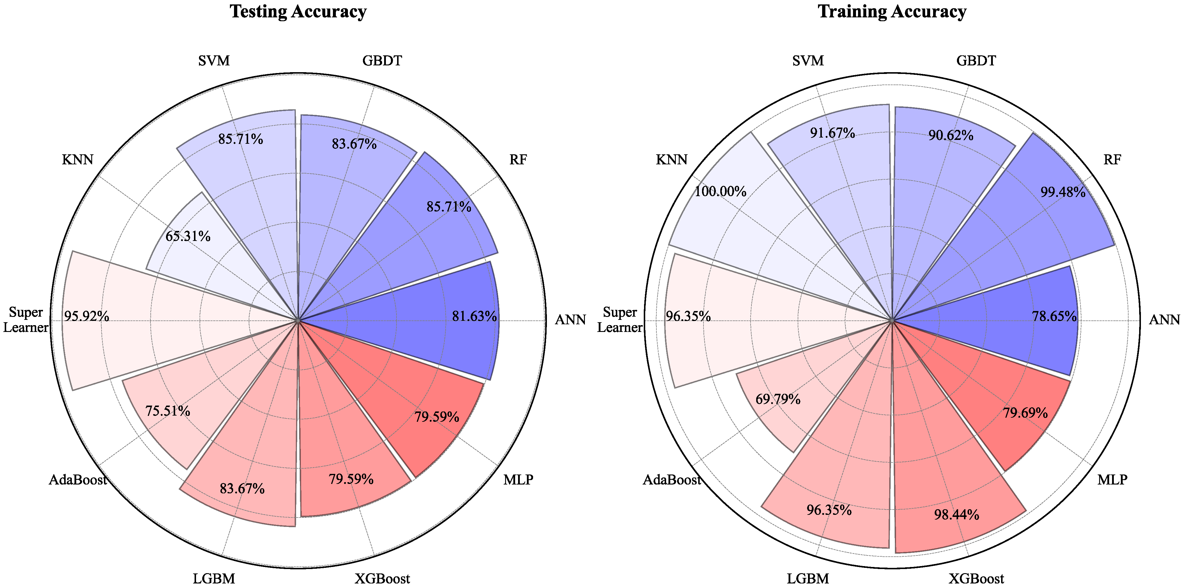
As shown in Figure 14, a comparison of the prediction results between various single models and the Super Learner model is presented, evaluated on both the training and test sets. The analysis reveals two key issues with the single models. First, their performance is generally suboptimal, often failing to produce satisfactory prediction results on the test set. Second, a significant overfitting problem is observed, with models performing well on the training set but poorly on the test set. Except for ANN, MLP, and AdaBoost, all other models exhibit some degree of overfitting, with KNN being particularly problematic. While KNN correctly predicted all samples in the training set, its accuracy on the test set was only 65.31%. In contrast, the Super Learner model employed in this study successfully addressed both of these issues, achieving the highest prediction accuracy of 95.92% on the test set, without exhibiting significant overfitting or underfitting.

5.1.3. Comparison with Other Studies

As shown in

Table 5. Comparison of model performance between this study and previous research.

Researcher	Year	Dataset Size	Test Set Size	ML Method	Hyperparameter Optimization	Accuracy (%)
Tawadrous and Katsabanis [18]	2007	100	30	ANN(MLP)	None	93.00%
Zhou et al. [39]	2015	251	74	SVM	Cross-Validation	82.40%
				RF		82.40%
				ANN		81.10%
				GBM		79.70%
				LDA		66.20%
				MLR		63.50%
Ghasemi et al. [22]	2017	178	27	J48	Grid Search	81.48%
				SVC		74.04%
Liang et al. [23]	2020	236	71	GBDT	Cross-Validation	83.10%
				XGBoost		83.10%
				LightGBM		81.69%
Li et al. [21]	2022	162	9	LMT	Cross-Validation	94.10%
Li et al. [24]	2023	306	92	GWO-SVM	GWO, WOA, SSA	90.22%
				WOA-SVM		89.96%
				SSA-SVM		91.30%
Kamran et al. [25]	2024	236	71	KNN-GWO	GWO	93.00%
This study	2025	241	49	BSMOTE-OOA-SL	OOA	95.92%

, a comparison between the BSMOTE-OOA-SL model used in this study and previous research on pillar stability prediction is presented. The results indicate that, despite the significant progress made by many novel methods and excellent models in the field, such as the introduction of metaheuristic algorithms by Li et al. [24] and Kamran et al. [25], or the adoption of innovative models by Li et al. [21] and Liang et al. [23], our approach still demonstrates unique advantages in terms of prediction accuracy, generalization, and the ability to handle complex, imbalanced datasets. The proposed ensemble learning framework in this study, compared to previous single-model approaches, is more adaptable to varying data environments, enabling more robust predictions. Furthermore, the combination of Borderline-SMOTE and OOA ensures that the model benefits not only from enhanced data representation but also from a stable improvement in performance. In conclusion, our proposed method provides a more robust solution for pillar stability prediction.

5.2. Model Interpretability Analysis

While predictive performance is crucial in model development, model interpretability is equally important. This is particularly significant in the task of pillar stability prediction, where safety is a critical concern in the mining industry. Being able to explain why a model predicts a particular outcome—such as whether a pillar is stable or unstable—can provide valuable insights for decision-makers and help guide safety protocols [53,54]. Therefore, a model interpretability framework of SHapley Additive exPlanations (SHAP), implemented using the Python SHAP library (version 0.44.1), is introduced to enhance our understanding of the prediction mechanism in pillar stability. This framework combines Shapley values from cooperative game theory with local interpretable model-agnostic explanations (LIME), using Shapley values to provide explanations for the predictions made by machine learning algorithms [30]. The interpretability of the model predictions is analyzed from the following three perspectives:

5.2.1. Global Feature Importance Analysis

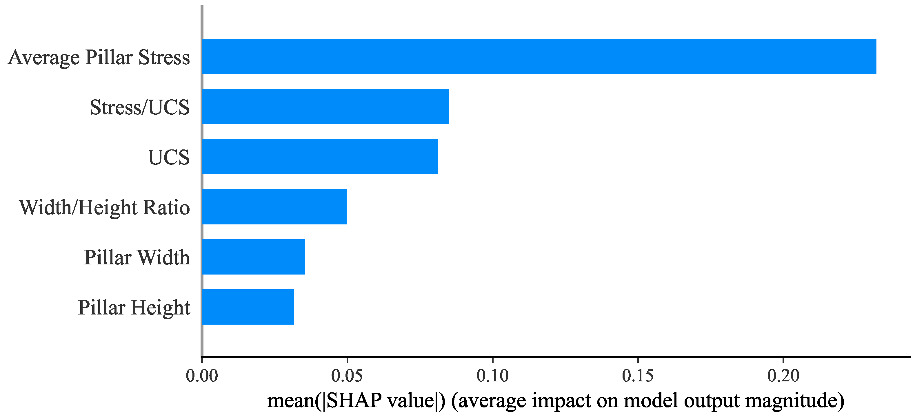
In the context of pillar stability classification, the “Failed” category is of primary focus, as accurately predicting this category is crucial for preventing accidents. To understand which features the model considers most important on a global level, the SHAP values are calculated by their contribution of input features on predictions of the “Failed” category.

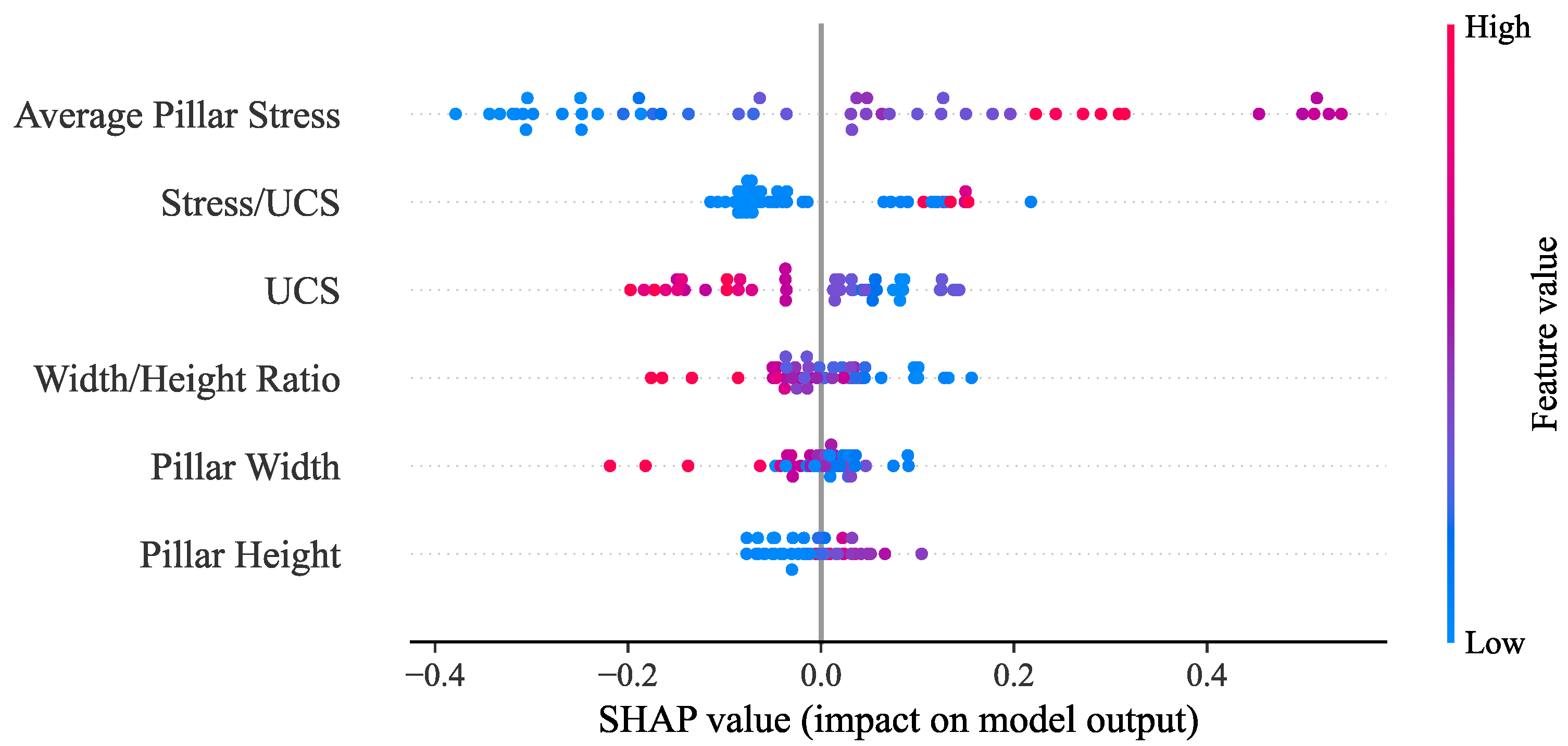
Figure 15 illustrates the global feature importance by calculating the average absolute value of the SHAP values for each feature, then ranking the features accordingly. The longer the bar, the greater the average impact that feature has on the model’s prediction. Figure 16 presents a more informative feature importance ranking, which not only shows the feature importance on the Y-axis but also reveals how the magnitude of the feature values affects the direction of the prediction. It is clear that the stress-related indicators play a critical role in predicting the “Failed” category. The most important feature is Average Pillar Stress, followed by Stress/UCS and UCS. This finding aligns well with engineering principles and the fundamental mechanisms of pillar instability. Rock pillar instability is primarily caused by high average stress on the pillar and stress concentration at weak points, which in turn leads to shear or tensile failure [55,56]. In particular, Average Pillar Stress serves as a direct indicator of the load carried by the pillar, while the Stress/UCS ratio and UCS provide insight into the pillar’s ability to resist failure under varying stress conditions.

5.2.2. Single Sample Prediction Explanation

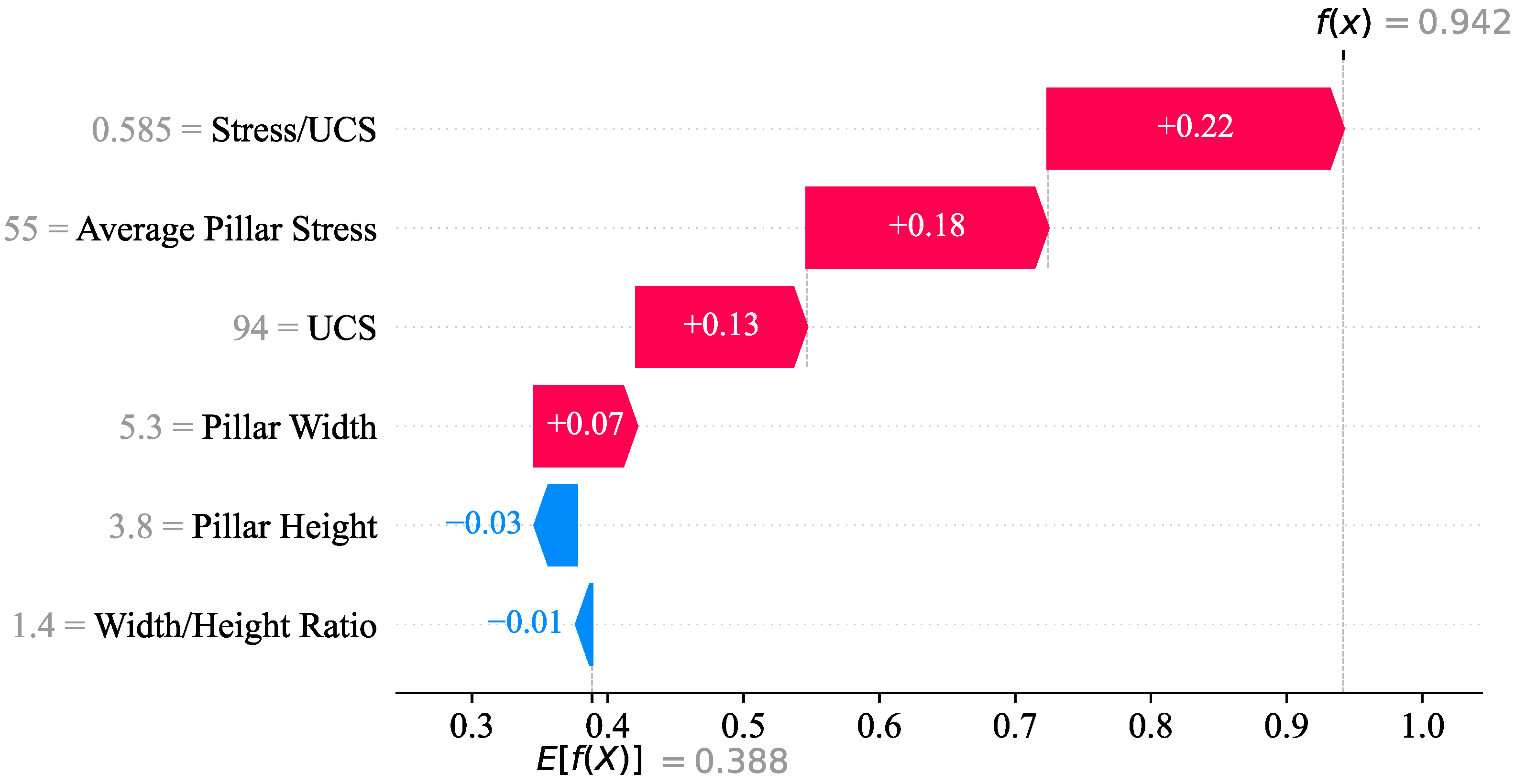
To explain the model’s prediction process for a single sample, an example selected from the test set is demonstrated in Figure 17. This plot clearly illustrates how the model’s baseline value (the average prediction for all samples) is gradually adjusted as each feature contributes to the final prediction. Each step in the waterfall plot shows the incremental effect of individual features on the prediction outcome. In this specific sample, the most influential feature is Stress/UCS, followed by Average Pillar Stress. Both features make substantial positive contributions to the prediction, increasing the predicted probability by +0.22 and +0.18, respectively. In contrast, features such as Pillar Height and the Pillar Width/Height Ratio exhibit negative contributions, slightly reducing the predicted probability by −0.03 and −0.01, respectively. Other features, such as UCS and Pillar Width, also contribute positively to the prediction, though their effects are smaller. By using SHAP values to quantify the contribution of each feature and providing local explanations for individual predictions, it is thoroughly investigated how specific features influence the given prediction. This significantly enhances the model’s interpretability, offering a clearer understanding of its decision-making process.

5.2.3. Multi-Sample Aggregated Explanation

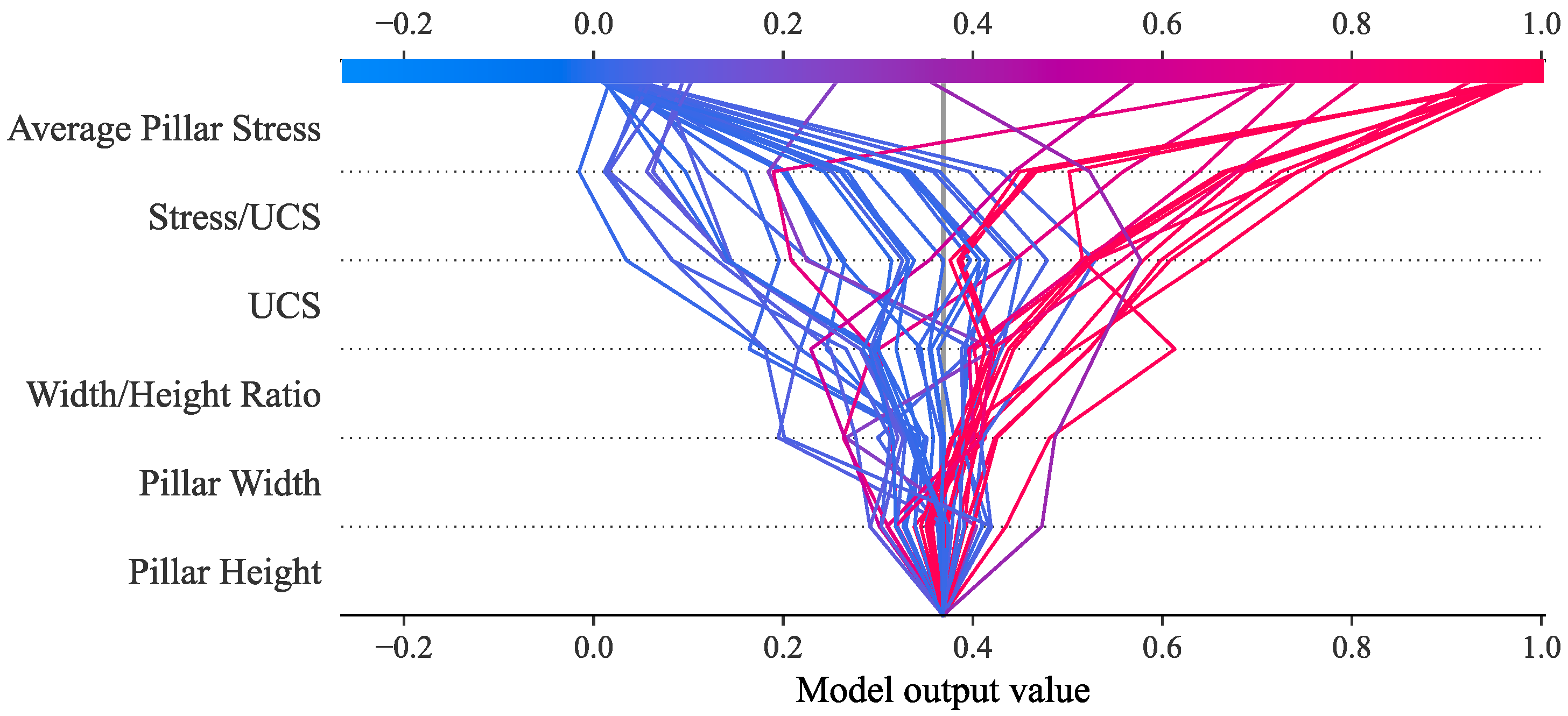
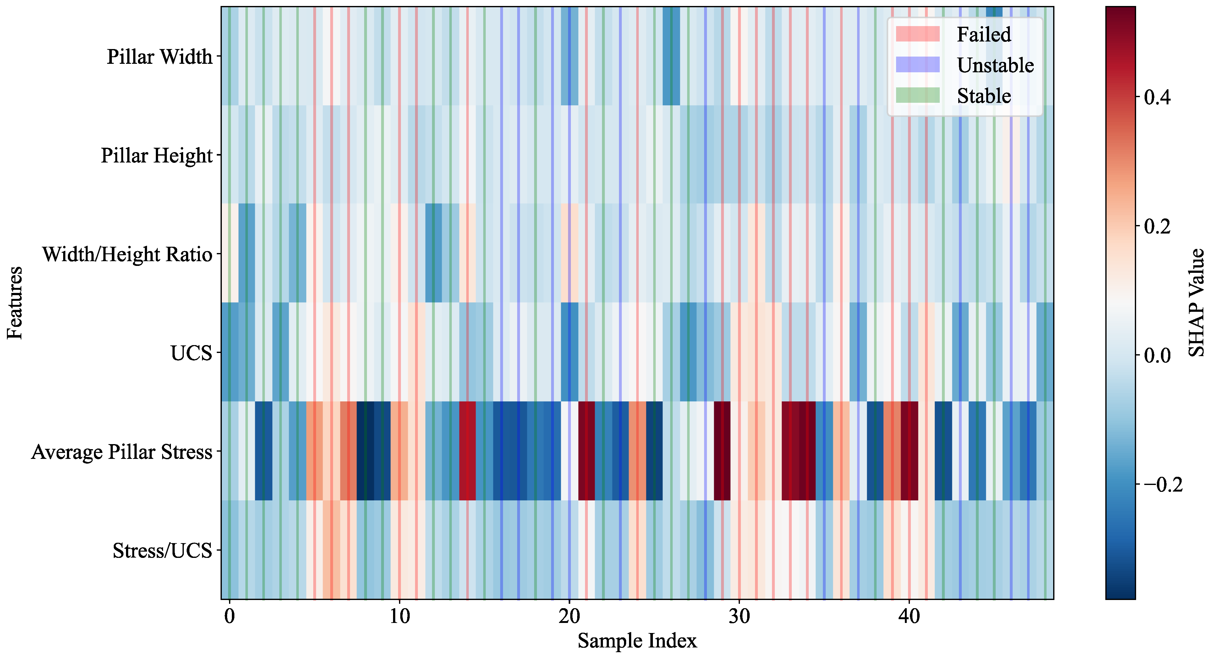
To better understand the model’s behavior across multiple samples, the multi-sample decision plot and SHAP heatmap were illustrated in Figure 18 and Figure 19. The decision plot stacks the waterfall plots of multiple samples, with each line representing the prediction path of an individual sample. Starting from the baseline value, the line shifts as each feature is added, ultimately arriving at the final prediction value for that sample. This visualization highlights the differences in decision paths across samples, emphasizing the varying impact of each feature on the model’s predictions. For instance, features like Average Pillar Stress may consistently push the prediction towards a dichotomous outcome, determining whether the pillar is categorized as “Failed” or not, whereas features like Pillar Width may cause fluctuations in the prediction. The SHAP heatmap represents the SHAP values of each sample and each feature as a matrix. The color intensity in the heatmap corresponds to the magnitude of the SHAP values, providing a clear view of how each feature influences the model’s output across different samples. This heatmap allows us to identify clusters of samples with similar feature contributions, revealing patterns that might not be immediately apparent from individual sample analysis.

Clearly, the interpretability analysis conducted on the model provides valuable insights for practical engineering applications. In pillar stability prediction, engineers require not only accurate predictions but also a clear understanding of the mechanisms behind these predictions. Such results and understanding can assist in safety decision-making and help formulate more effective preventive measures. Based on the above analysis, both global and local explanations highlight that stress-related indicators should receive increased attention. Significant changes in these indicators can notably influence the final prediction outcome. From an engineering perspective, the variation of these indicators can be further investigated through numerical simulation or field measurements. In this way, mitigation strategies to reduce potential risks can then be designed. For example, decompression techniques can be applied to pillars already at risk of instability, reducing the risk associated with high stress indicators [57,58,59]. In summary, the insights provided by SHAP can guide more informed decision-making in pillar design and maintenance.

5.3. Limitations

While this study achieves notable advancements in the field of pillar stability prediction, there are still some limitations that need to be addressed.

(1)

The diversity and reliability of the data still require further improvement. Due to the limited number of training samples available in this study and the presence of noticeable class imbalance, the applicability of the proposed model is mainly confined to specific hard rock pillar scenarios. Although cross-validation, Borderline-SMOTE, and ensemble learning were employed to mitigate these issues, and the model has demonstrated significant improvements compared with existing approaches, the inherent biases and challenges in data collection and statistical representation still limit the coverage of diverse pillar conditions across different mining environments. Therefore, the results should be interpreted within the context of the available data. Future data collection efforts should focus on expanding the dataset size and the range of operating conditions to further enhance the model’s generalizability.

(2)

The study of features in pillar stability prediction requires further investigation. In the model interpretability analysis, it is revealed that many features had a relatively small contribution to the model’s predictions. Given the current data resources, future research should focus on utilizing feature fusion techniques to extract more meaningful information from the existing features. By combining or deriving new features, the model’s predictive power can be further enhanced. Additionally, future data collection efforts should consider incorporating more key features, such as geological characteristics, mining methods, and pillar geometry, as these factors may provide additional insights into pillar stability prediction.

6. Conclusions

Pillar stability prediction is essential for ensuring the safety and operational efficiency of underground mining systems, particularly under conditions of increasing mining depth and geological complexity. To address the challenges associated with small sample sizes, pronounced class imbalance, and limited interpretability in existing data-driven approaches, this study proposed an integrated BSMOTE-OOA-Super Learner (BSMOTE-OOA-SL) framework for hard-rock pillar stability prediction. Based on the comprehensive experimental results and analyses presented in this study, the main conclusions are summarized as follows:

(1)

A dataset comprising 241 hard-rock pillar cases collected from seven underground mines was established, exhibiting substantial heterogeneity and class imbalance. To ensure statistical reliability, the performance of all models was evaluated using repeated experiments with multiple random train-test splits. The results show that the BSMOTE-OOA-SL model consistently outperforms individual base learners in terms of overall Accuracy, Macro-Precision, Macro-Recall, and Macro-F1. In addition, the relatively small standard deviations of these metrics indicate that the proposed framework provides stable and reliable predictions across different data partitions, highlighting its robustness and generalization capability in data-scarce scenarios.

(2)

Based on a representative train-test split selected for detailed analysis, the proposed BSMOTE-OOA-SL model attains a high overall classification accuracy of 95.92%. More importantly, the model exhibits consistently strong class-wise Precision, Recall, and F1-score for all pillar stability categories (Stable, Unstable, and Failed). The ROC analysis further confirms its discriminative effectiveness, with AUC values exceeding 0.9 for all classes and reaching 1.0 for the Failed category. These results indicate that, beyond achieving strong average performance, the proposed framework is capable of reliably identifying high-risk stability states that are critical for mining safety.

(3)

Ablation experiments demonstrate that both Borderline-SMOTE and the Osprey Optimization Algorithm contribute positively to model performance, with Borderline-SMOTE providing a more pronounced improvement due to the severe class imbalance of the dataset. When the two techniques are jointly employed, the proposed framework achieves clear quantitative performance gains: compared with the baseline model without BSMOTE and OOA, Accuracy, Macro-Precision, Macro-Recall, and Macro-F1 increase by 10.21%, 12.25%, 12.61%, and 12.86%, respectively. These results confirm that combining targeted oversampling within training folds with systematic hyperparameter optimization is essential for improving predictive accuracy, stability, and reliability.

(4)

The application of SHapley Additive exPlanations (SHAP) enables transparent interpretation of the proposed model at both global and local levels. The interpretability results consistently identify stress-related indicators—particularly average pillar stress, Stress/UCS ratio, and UCS—as the dominant factors influencing pillar stability predictions, especially for the Failed category. These findings are well aligned with established rock mechanics principles, enhancing confidence in the physical plausibility and engineering relevance of the proposed framework. Such interpretability facilitates informed decision-making and supports the practical integration of machine learning predictions into pillar design and safety management.

In summary, this study presents a robust, interpretable, and statistically reliable hybrid framework for pillar stability prediction. By explicitly addressing class imbalance, optimizing model hyperparameters, and providing physically consistent explanations of model behavior, the proposed BSMOTE-OOA-SL framework offers a practical and effective tool for underground hard-rock pillar stability assessment and mining safety management.

References

1. Dismuke, S.R.; Forsyth, W.W.; Stewart, S.B.V. The evolution of mining strategy following the collapse of the window area at the Magmont Mine, Missouri. In Proceedings of the CIM Annual General Meeting, District 6, Metal Mining, Toronto, ON, Canada, 1–4 May 1994; Canadian Institute of Mining (CIM): Montreal, QC, Canada, 1994; pp. 3–8. [Google Scholar]
2. Zhou, Z.; Zang, H.; Cao, W.; Du, X.; Chen, L.; Ke, C. Risk assessment for the cascading failure of underground pillar sections considering interaction between pillars. Int. J. Rock Mech. Min. Sci. 2019, 124, 104142. [Google Scholar] [CrossRef]
3. Zipf, R.K. Toward pillar design to prevent collapse of room-and-pillar mines. In Proceedings of the 108th Annual Exhibit and Meeting, Krakow, Poland, 17–22 June 2001; Society for Mining, Metallurgy and Exploration: Denver, CO, USA, 2001; pp. 1–11. [Google Scholar]
4. Nordlund, E.; Radberg, G.; Jing, L. Determination of failure modes in jointed pillars by numerical modelling. In Proceedings of the Conference on Fractured and Jointed Rock Masses, Lake Tahoe, CA, USA, 3 June 1992; Taylor & Francis: Washington, DC, USA, 1995; pp. 345–350. [Google Scholar]
5. Esterhuizen, G.S.; Dolinar, D.R.; Ellenberger, J.L. Pillar strength in underground stone mines in the United States. Int. J. Rock Mech. Min. Sci. 2011, 48, 42–50. [Google Scholar] [CrossRef]
6. Hoek, E.; Carranza-Torres, C.; Corkum, B. Hoek-Brown failure criterion—2002 Edition. Proc. NARMS-Tac 2002, 1, 267–273. [Google Scholar]
7. Bieniawski, Z.T. A method revisited: Coal pillar strength formula based on field investigations. In Proceedings of the Workshop on Coal Pillar Mechanics and Design, Santa Fe, NM, USA, 7 June 1992; US Department of the Interior, Bureau of Mines, IC: Pittsburgh, PA, USA, 1992; Volume 9315, pp. 158–165. [Google Scholar]
8. Wang, X.; Guan, K.; Yang, T.; Liu, X. Instability mechanism of pillar burst in asymmetric mining based on cusp catastrophe model. Rock Mech. Rock Eng. 2021, 54, 1463–1479. [Google Scholar] [CrossRef]
9. Jiang, L.; Jiao, H.; Xie, B.; Yang, H. Study on safety coefficient of sedimentary bauxite strip pillar under valley terrain. Int. J. Environ. Res. Public Health 2022, 19, 10991. [Google Scholar] [CrossRef]
10. Zhang, H.; Liu, G.; Liu, W.; Chen, Z.; Miao, Z.; Liu, Q. Stability evaluation of rock pillar between twin tunnels using the YAI. Sci. Rep. 2023, 13, 13187. [Google Scholar] [CrossRef]
11. Ju, F.; Wang, D.; Wang, Z. Coal Pillar Stability Investigation for high-intensity mining in the water-rich coal seam: A case study. Min. Metall. Explor. 2024, 41, 743–768. [Google Scholar] [CrossRef]
12. Kaiser, P.K.; Tang, C.A. Numerical simulation of damage accumulation and seismic energy release during brittle rock failure—Part II: Rib Pillar Collapse. Int. J. Rock Mech. Min. Sci. 1998, 35, 123–134. [Google Scholar] [CrossRef]
13. Hauquin, T.; Gunzburger, Y.; Deck, O. Predicting pillar burst by an explicit modelling of kinetic energy. Int. J. Rock Mech. Min. Sci. 2018, 107, 159–171. [Google Scholar] [CrossRef]
14. Yu, Y.; Chen, S.; Deng, K.; Fan, H. Long-term stability evaluation and pillar design criterion for room-and-pillar mines. Energies 2017, 10, 1644. [Google Scholar] [CrossRef]
15. Elmo, D.; Stead, D. An integrated numerical modelling–discrete fracture network approach applied to the characterization of rock mass strength of naturally fractured pillars. Rock Mech. Rock Eng. 2010, 43, 3–19. [Google Scholar] [CrossRef]
16. Li, C.; Zhou, J.; Armaghani, D.J.; Li, X. Stability analysis of underground mine hard rock pillars via combination of finite difference methods, neural networks, and Monte Carlo simulation techniques. Undergr. Space 2021, 6, 379–395. [Google Scholar] [CrossRef]
17. Deng, J.; Yue, Z.Q.; Tham, L.G.; Zhu, H.H. Pillar Design by combining finite element methods, neural networks and reliability: A case study of the Feng Huangshan copper mine, China. Int. J. Rock Mech. Min. Sci. 2003, 40, 585–599. [Google Scholar] [CrossRef]
18. Tawadrous, A.S.; Katsabanis, P.D. Prediction of surface crown pillar stability using artificial neural networks. Int. J. Numer. Anal. Methods Geomech. 2007, 31, 917–931. [Google Scholar] [CrossRef]
19. Zhou, J.; Li, X.; Shi, X.; Wei, W.; Wu, B. Predicting Pillar stability for underground mine using fisher discriminant analysis and SVM methods. Trans. Nonferrous Met. Soc. China 2011, 21, 2734–2743. [Google Scholar] [CrossRef]
20. Wattimena, R.K.; Kramadibrata, S.; Sidi, I.D.; Azizi, M.A. Developing coal pillar stability chart using logistic regression. Int. J. Rock Mech. Min. Sci. 2013, 58, 55–60. [Google Scholar] [CrossRef]
21. Li, N.; Zare, M.; Yi, C.; Jimenez, R. Stability risk assessment of underground rock pillars using logistic model trees. Int. J. Environ. Res. Public Health 2022, 19, 2136. [Google Scholar] [CrossRef]
22. Ghasemi, E.; Kalhori, H.; Bagherpour, R. Stability assessment of hard rock pillars using two intelligent classification techniques: A comparative study. Tunn. Undergr. Space Technol. 2017, 68, 32–37. [Google Scholar] [CrossRef]
23. Liang, W.; Luo, S.; Zhao, G.; Wu, H. Predicting hard rock pillar stability using GBDT, XGBoost, and LightGBM algorithms. Mathematics 2020, 8, 765. [Google Scholar] [CrossRef]
24. Li, C.; Zhou, J.; Du, K.; Dias, D. Stability prediction of hard rock pillar using support vector machine optimized by three metaheuristic algorithms. Int. J. Min. Sci. Technol. 2023, 33, 1019–1036. [Google Scholar] [CrossRef]
25. Kamran, M.; Chaudhry, W.; Taiwo, B.O.; Hosseini, S.; Rehman, H. Decision intelligence-based predictive modelling of hard rock pillar stability using k-nearest neighbour coupled with grey wolf optimization algorithm. Processes 2024, 12, 783. [Google Scholar] [CrossRef]
26. Shaaban, M.; Amin, M.; Selim, S.; Riad, I.M. Machine Learning Approaches for Forecasting Compressive Strength of High-Strength Concrete. Sci. Rep. 2025, 15, 25567. [Google Scholar] [CrossRef] [PubMed]
27. Amin, M.; El-hassan, K.A.; Shaaban, M.; Mashaly, A.A. Effect of Waste Tea Ash and Sugar Beet Waste Ash on Green High Strength Concrete. Constr. Build. Mater. 2025, 495, 143611. [Google Scholar] [CrossRef]
28. Zhou, Z.-H. Ensemble Methods: Foundations and Algorithms; CRC Press: Boca Raton, FL, USA, 2025; ISBN 978-1-040-30763-2. [Google Scholar]
29. Talbi, E.-G. Metaheuristics: From Design to Implementation; John Wiley & Sons: Hoboken, NJ, USA, 2009; ISBN 978-0-470-49690-9. [Google Scholar]
30. Salih, A.M.; Raisi-Estabragh, Z.; Galazzo, I.B.; Radeva, P.; Petersen, S.E.; Lekadir, K.; Menegaz, G. A perspective on explainable artificial intelligence methods: SHAP and LIME. Adv. Intell. Syst. 2025, 7, 2400304. [Google Scholar] [CrossRef]
31. Hedley, D.F.G. Stope-and-Pillar Design for the Elliot Lake Uranium Mines; Stope-and-Pillar Design; Elliot Lake Uranium Mines: Elliot Lake, ON, Canada, 1972. [Google Scholar]
32. Von Kimmelmann, M.R.; Hyde, B.; Madgwick, R.J. 7 the Use of Computer Applications at BCL Limited in Planning Pillar Extraction and the Design of Mining Layouts. In Proceedings of the Design and Performance of Underground Excavations: ISRM Symposium, Cambridge, UK, 3–6 September 1984; Brown, E.T., Hudson, J.A., Eds.; Emerald Publishing Limited: Bradford, UK, 1984; pp. 53–63. ISBN 978-0-7277-4008-3. [Google Scholar]
33. Potvin, Y.; Hudyma, M.; Miller, H.D.S. Rib Pillar Design in Open Stope Mining. Bull. Can. Inst. Min. Met. 1989, 82, 31–36. [Google Scholar]
34. Sjoberg, J.S. Failure Modes and Pillar Behaviour in the Zinkgruvan Mine. In Proceedings of the ARMA US Rock Mechanics/Geomechanics Symposium, Santa Fe, NM, USA, 3–5 June 1992; ARMA–92-0491. OnePetro: Houston, TX, USA, 1992; pp. 1–10. [Google Scholar]
35. Lunder, P.J. Hard Rock Pillar Strength Estimation an Applied Empirical Approach. Ph.D. Thesis, University of British Columbia, Vancouver, BC, Canada, 1994. [Google Scholar]
36. González-Nicieza, C.; Álvarez-Fernández, M.I.; Menéndez-Díaz, A.; Álvarez-Vigil, A.E. A comparative analysis of pillar design methods and its application to marble mines. Rock Mech. Rock Eng. 2006, 39, 421–444. [Google Scholar] [CrossRef]
37. Wattimena, R.K. Predicting the stability of hard rock pillars using multinomial logistic regression. Int. J. Rock Mech. Min. Sci. 2014, 71, 33–40. [Google Scholar] [CrossRef]
38. Schubert, C.; Villaescusa, E. An approach to hard rock pillar design at the McArthur River Mine. In Proceedings of the AusIMM Annual Conference, Mount Isa, Queensland, Australia, 19–23 April 1998; pp. 255–259. [Google Scholar]
39. Zhou, J.; Li, X.; Mitri, H.S. Comparative performance of six supervised learning methods for the development of models of hard rock pillar stability prediction. Nat. Hazard. 2015, 79, 291–316. [Google Scholar] [CrossRef]
40. Van der Laan, M.; Polley, E.; Hubbard, A. Super Learner. Stat. Appl. Genet. Mol. Biol. 2007, 6, 1309. [Google Scholar] [CrossRef]
41. Van Der Laan, M.J.; Rose, S. Targeted Learning: Causal Inference for Observational and Experimental Data; Springer Series in Statistics; Springer: New York, NY, USA, 2011; ISBN 978-1-4419-9781-4. [Google Scholar]
42. Dehghani, M.; Trojovský, P. Osprey optimization algorithm: A new bio-inspired metaheuristic algorithm for solving engineering optimization problems. Front. Mech. Eng. 2023, 8, 1126450. [Google Scholar] [CrossRef]
43. Han, H.; Wang, W.-Y.; Mao, B.-H. Borderline-SMOTE: A New over-Sampling method in imbalanced data sets learning. In Proceedings of the Advances in Intelligent Computing, Hefei, China, 23–26 August 2005; Huang, D.-S., Zhang, X.-P., Huang, G.-B., Eds.; Springer: Berlin/Heidelberg, Germany, 2005; pp. 878–887. [Google Scholar]
44. Naimi, A.I.; Balzer, L.B. Stacked Generalization: An Introduction to Super Learning. Eur. J. Epidemiol. 2018, 33, 459–464. [Google Scholar] [CrossRef] [PubMed]
45. Santos, M.S.; Soares, J.P.; Abreu, P.H.; Araujo, H.; Santos, J. Cross-validation for imbalanced datasets: Avoiding overoptimistic and overfitting approaches [Research Frontier]. IEEE Comput. Intell. Mag. 2018, 13, 59–76. [Google Scholar] [CrossRef]
46. Demircioğlu, A. Applying oversampling before cross-validation will lead to high bias in radiomics. Sci. Rep. 2024, 14, 11563. [Google Scholar] [CrossRef] [PubMed]
47. Hossin, M.; Sulaiman, M.N. A review on evaluation metrics for data classification evaluations. Int. J. DATA Min. Knowl. Manag. Process 2015, 5, 1–11. [Google Scholar] [CrossRef]
48. Mujahid, M.; Kına, E.; Rustam, F.; Villar, M.G.; Alvarado, E.S.; De La Torre Diez, I.; Ashraf, I. Data oversampling and imbalanced datasets: An investigation of performance for machine learning and feature engineering. J. Big DATA 2024, 11, 87. [Google Scholar] [CrossRef]
49. Bischl, B.; Binder, M.; Lang, M.; Pielok, T.; Richter, J.; Coors, S.; Thomas, J.; Ullmann, T.; Becker, M.; Boulesteix, A.-L.; et al. Hyperparameter optimization: Foundations, algorithms, best practices, and open challenges. WIREs Data Min. Knowl. Discov. 2023, 13, e1484. [Google Scholar] [CrossRef]
50. Alvarez-Garcia, I.N.; Ramos-Lopez, F.L.; Gonzalez-Nicieza, C.; Alvarez-Fernandez, M.I.; Alvarez-Vigil, A.E. The Mine Collapse at Lo Tacón (Murcia, Spain), Possible Cause of the Torre Pacheco Earthquake (2nd May 1998, SE Spain). Eng. Fail. Anal. 2013, 28, 115–133. [Google Scholar] [CrossRef]
51. Schwenker, F. Ensemble Methods: Foundations and Algorithms [Book Review]. IEEE Comput. Intell. Mag. 2013, 8, 77–79. [Google Scholar] [CrossRef]
52. Ardabili, S.; Mosavi, A.; Várkonyi-Kóczy, A.R. Advances in Machine Learning Modeling Reviewing Hybrid and Ensemble Methods. In Proceedings of the Engineering for Sustainable Future, Budapest and Balatonfüred, Hungary, 4–7 September 2019; Várkonyi-Kóczy, A.R., Ed.; Springer International Publishing: Cham, Switzerland, 2020; pp. 215–227. [Google Scholar]
53. Du, M.; Liu, N.; Hu, X. Techniques for Interpretable Machine Learning. Commun. ACM 2019, 63, 68–77. [Google Scholar] [CrossRef]
54. Rudner, T.; Toner, H. Key Concepts in AI Safety: Interpretability in Machine Learning; Center for Security and Emerging Technology: Washington, DC, USA, 2021; pp. 1–8. [Google Scholar]
55. Martin, C.D.; Maybee, W.G. The strength of hard-rock pillars. Int. J. Rock Mech. Min. Sci. 2000, 37, 1239–1246. [Google Scholar] [CrossRef]
56. Sun, L.; Ye, Y.; Luo, B.; Hu, N.; Li, P. Theoretical analysis for stability evaluation of rock mass engineering structure under combined compression-shear loading: A case study of inclined pillar. Appl. Sci. 2021, 11, 11439. [Google Scholar] [CrossRef]
57. Lei, W.; Chai, J.; Liu, J.; Cao, Y.; Yuchi, X.; Zhang, D.; Zheng, C.; Du, X.; Gong, Y. Research on stress release and pressure relief mechanism of underlying coal and rock under protective layer mining. Sci. Rep. 2025, 15, 5583. [Google Scholar] [CrossRef]
58. Ranjbarnia, M.; Oreste, P.; Fahimifar, A. The Rock Pillar Stress Analysis in order to obtain an effective dimensioning and guarantee the mining void stability. Sci. Iran. 2018, 25, 543–556. [Google Scholar] [CrossRef]
59. Xia, K.; Chen, C.; Liu, X.; Liu, X.; Yuan, J.; Dang, S. Assessing the stability of high-level pillars in deeply-buried metal mines stabilized using cemented backfill. Int. J. Rock Mech. Min. Sci. 2023, 170, 105489. [Google Scholar] [CrossRef]
Figure 1. Pillar stability classification.
Symmetry 18 00049 g001
Figure 2. Distribution of pillar stability states across mines and overall dataset.
Symmetry 18 00049 g002
Figure 3. Feature correlation matrix and class-wise distributions for pillar stability dataset.
Symmetry 18 00049 g003
Figure 4. Flow chart of Super Learner.
Symmetry 18 00049 g004
Figure 5. Flow chart of OOA.
Symmetry 18 00049 g005
Figure 6. Flow chart of pillar stability prediction.
Symmetry 18 00049 g006
Figure 7. Schematic of the confusion matrix for a three-class classification problem.
Symmetry 18 00049 g007
Figure 8. Schematic representation of the ROC curve.
Symmetry 18 00049 g008
Figure 9. Accuracy variation of base learners and BSMOTE-OOA-SL across 20 random test splits.
Symmetry 18 00049 g009
Figure 10. Convergence curves of OOA hyperparameter optimization for base learners.
Symmetry 18 00049 g010aSymmetry 18 00049 g010b
Figure 11. BSMOTE-OOA-SL confusion matrix and ROC curve on test set.
Symmetry 18 00049 g011
Figure 12. Impact of OOA and Borderline-SMOTE on model performance.
Symmetry 18 00049 g012
Figure 13. Impact of OOA and Borderline-SMOTE on classification metrics across classes.
Symmetry 18 00049 g013
Figure 14. Comparison of Super Learner ensemble model and single models.
Symmetry 18 00049 g014
Figure 15. SHAP summary plot of “Failed” category.
Symmetry 18 00049 g015
Figure 16. SHAP beeswarm plot of “Failed” category.
Symmetry 18 00049 g016
Figure 17. SHAP waterfall plot of a certain sample.
Symmetry 18 00049 g017
Figure 18. Multi-sample decision plot.
Symmetry 18 00049 g018
Figure 19. SHAP heatmap.
Symmetry 18 00049 g019