The Analysis of Three-Dimensional Time-Fractional Helmholtz Model Using a New İterative Method

Abstract

This paper proposes a novel analytical method to address the Helmholtz fractional differential equation by combining the Aboodh transform with the Adomian Decomposition Method, resulting in the Aboodh–Adomian Decomposition Method (A-ADM). Fractional differential equations offer a comprehensive framework for describing intricate physical processes, including memory effects and anomalous diffusion. This work employs the Caputo–Fabrizio fractional derivative, defined by a non-singular exponential kernel, to more precisely capture these non-local effects. The classical Helmholtz equation, pivotal in acoustics, electromagnetics, and quantum physics, is extended to the fractional domain. Following the exposition of fundamental concepts and characteristics of fractional calculus and the Aboodh transform, the suggested A-ADM is employed to derive the analytical solution of the fractional Helmholtz equation. The method’s validity and efficiency are evidenced by comparisons of analytical and approximation solutions. The findings validate that A-ADM is a proficient and methodical approach for addressing fractional differential equations that incorporate Caputo–Fabrizio derivatives.

1. Introduction

Fractional differential equations (PDEs) serve as powerful tools for modeling many physical, technological, and biological systems, distinguished by the generalization of traditional differentiation and integration methods to fractional orders. The additional degrees of freedom provided by fractional derivatives facilitate the modeling of memory and persistence effects, resulting in more accurate solutions to situations that conventional differential equations cannot clarify.

The Helmholtz differential equation is a crucial partial differential equation in disciplines such as acoustics, electromagnetic theory, quantum physics, and optics. The use of this equation for fractional-order derivatives facilitates more realistic modeling of physical systems and enhances prediction accuracy, particularly in anisotropic and heterogeneous media.

In this paper, an analytical solution to the Helmholtz fractional differential equation is obtained using an Aboodh transform-based approach. The Aboodh transform is a powerful integral transform technique that is comparable to the classical Laplace transform and simplifies the resolution of differential equations. The Aboodh transform has been successfully utilized in several physical issues documented in the literature. This research evaluates its effectiveness in solving the Helmholtz fractional differential equation.

The analytical solution of two-dimensional fractional Helmholtz equations using FRDTM was obtained by Abuasad et al. [1]. Ghaffar et al. employed the multi-grid method in [2] to solve the 3D Helmholtz equation using higher-order compact difference (Hoc) schemes. Gupta et al. [3] employed the homotopy perturbation method of He to resolve the multidimensional fractional Helmholtz equation. Li [4] presented a fast singular boundary method (SBM) for the three-dimensional (3D) Helmholtz equation. Li et al. [5] proposed a systematic method to assess the near-boundary and boundary solutions for the three-dimensional Helmholtz equation with broad-band wavenumbers. Bespalov et al. [6] introduced the adaptive boundary element approach exhibiting optimal convergence rates for the 2D and 3D Helmholtz problems. A novel finite difference approach for the solution of the Helmholtz equation in polar and spherical dimensions was introduced by Wang et al. in [7]. Qu et al. in [8] introduced the fast multipole accelerated singular boundary method (SBM) for solving the large-scale three-dimensional Helmholtz equation at low frequencies. Alshammari et al. [9] used the fractional reduced differential transform method (FRDTM) to obtain accurate solutions to the three-dimensional fractional Helmholtz equation (FHE). Nadem et al. [10] employed a new iterative method that integrates the Sumudu transformation method with the HPM method to conduct a prospective analysis of the three-dimensional time-fractional Helmholtz model. Nadem et al. [11] performed a numerical analysis of the two-dimensional fractional-time Helmholtz model with a novel iterative method that combines the Abood transform methodology with the HPM approach. Shah et al. [12] proposed a hybrid approach utilizing the Elzaki transform and HPS to obtain series solutions for fractional-order issues.

The primary advantages of the Caputo–Fabrizio derivative are its computational simplicity, owing to its non-singular kernel, and its capacity to offer more accurate representations of physical processes due to the near-memory effect. Ultimately, it may be readily modified to address many challenges in engineering and applied sciences. This derivative, first proposed by Caputo and Fabrizio [13], was created to overcome computational and physical incompatibilities caused by the singular kernels of traditional fractional derivatives. Losada et al. [14] conducted investigations examining the fundamental features of the Caputo–Fabrizio derivative, as well as the criteria for its existence and singularity as an operator. In the work referenced in [15], Atangana et al. examined diffusion models using the fractional derivative of Caputo–Fabrizio. In the article by Oprzedkiewic et al. [16], the authors used Caputo and Caputo–Fabrizio operators in modeling the heat transfer process.

In the following sections of this paper, the basic definitions of fractional derivatives and the Aboodh transform will first be discussed, followed by the steps towards the solution of the Helmholtz fractional differential equation. The aim of this paper is to consider the Caputo–Fabrizio fractional derivative with respect to the spatial variable x by capturing the non-local and memory effects found in physical phenomena such as wave propagation and diffusion in complex media of the following types:

$${}_0{}^{CF}D_x^{\alpha }u\left(x,y,t\right)+{\displaystyle \frac{{\partial }^2}{\partial y^2}}u\left(x,y,t\right)+{\displaystyle \frac{{\partial }^2}{\partial t^2}}u\left(x,y,t\right)+\gamma u\left(x,y,t\right)=0, 0<\alpha \le 1$$

(1)

with initial condition $u\left(x,y,t\right)=f\left(yt\right)$, where $f\left(yt\right)$ is a given function and $1 \le \alpha \le 2$.

This study aims to derive the precise solution for the 3D fractional Helmholtz equation using a novel approach and to find its fourth-order approximation solutions for different values of fractional derivatives. This work uniquely aims to delineate the Abood-ADM for the 3D Helmholtz equation through modest, sequential steps; consequently, this research serves as a fundamental reference for scholars to comprehend this method and implement it across various applications to achieve both exact and approximate solutions with minimal complexity.

The Aboodh transform is a commonly utilized method for transforming fractional differential equations, heat transfer, stochastic processes, and engineering applications. The Aboodh transform was initially introduced by Aboodh K.S in 2013 [17,18]. Benattia et al. [19] also solved the delay equations with the help of the Aboodh transform. Yasin et al. [20] solved the Newell–Whitehead–Segel Equations with the help of the Aboodh–ADM transform. Yasmin [21] used the Aboodh Homotopy Perturbation Transform Method for the fractional-order convection–reaction–diffusion equation utilizing Caputo and Atangana–Baleanu operators. Alshehry et al. [22] conducted a fractional-order appearance analysis of the Fisher and foam drainage equations using the Aboodh transform. Iqbal et al. [23] derived analytical solutions for the modified Korteweg–de Vries equation and associated Burger equations via the Aboodh transform. Ojo et al. [24] derived solutions using the Aboodh Transform Iterative Method for the spatial distribution of a biological population with fractional order.

Section 2 provides fundamental definitions in this investigation. Section 3 presents the methods and materials, Section 4 provides the convergence analysis, and Section 5 discusses the solutions and analysis of the Helmholtz problem as a novel application of the ATDM technique. Section 6 presents the results and discussions.

2. Preliminaries

Here we present some basic definitions of Caputo–Fabrizio that are important to our research.

Definition 1. 

Caputo–Fabrizio fractional derivative [25] of function $\mathcal{h}\left(t\right)$:

$${}_a{}^{CF}D_t^{\alpha }\mathcal{h}\left(t\right)={\displaystyle \frac{P\left(\alpha \right)}{1-\alpha }} {\int }_a^t{\mathcal{h}}^{\prime }(\tau )e^{\left[{\displaystyle \frac{-\alpha \left(t-\tau \right)}{1-\alpha }}\right]}d\tau , 0<\alpha \le 1$$

${\mathcal{h}}^{\prime } ϵ H^{\prime } \left(a,b\right), b>0$ and $P\left(\alpha \right)$ is the normalization constant depending on $a$, where $P\left(0\right)=P\left(1\right)=1$.

Definition 2. 

Caputo fractional derivative of $\mathcal{h}\left(t\right)$, where $\alpha >0$ is the order of the Caputo fractional derivative [26,27,28]:

$${}^{c}D_t^{\alpha }\mathcal{h}\left(t\right)=\left\{\begin{array}{c}{\displaystyle \frac{1}{\mathsf{Г}\left(p-\alpha \right)}}{\int }_0^t{\left(t-s\right)}^{p-\alpha -1}{\mathcal{h}}^{\left(p\right)}\left(s\right)ds, p-1<\alpha \le p \\ {\displaystyle \frac{{\partial }^n}{\partial t^n}}\mathcal{h}\left(t\right), \alpha =nϵ\mathbb{N} \\ \end{array}\right.$$

It is defined as follows:

Definition 3. 

The functions in the set $\mathcal{A}$ described as follows are taken into consideration by a new transformation for exponential functions known as the Aboodh transformation [17,18,19,20,21,22,23,24]:

$$\mathcal{A}=\left\{\mathcal{h}\left(t\right): \exists M, k_1, k_2>0, \left|\mathcal{h}\left(t\right)\right|<M{e}^{-st}\right\}$$

Aboodh transform of function $\mathcal{h}\left(t\right)$:

$$\mathcal{A}\left\{\mathcal{h}\left(t\right)\right\}=\mathcal{A}\{h(s)\}={\displaystyle \frac{1}{s}} {\int }_0^{\infty }\mathcal{h}\left(t\right)e^{-st} dt , t \ge 0 , k_1 \le s \le k_2$$

It is defined as follows:

Definition 4. 

Laplace Transform of Caputo–Fabrizio fractional derivative [29,30]:

$$L\left(s\right)={\displaystyle \frac{s^{n+1} L\left\{\mathcal{h}\left(t\right)\right\}-\mathcal{h}\left(0\right)s^n-{\mathcal{h}}^{\prime }\left(0\right)s^{n-1}-\cdots -{\mathcal{h}}^{\left(n\right)}\left(0\right)}{s+\alpha (1-s)}} , 0<\alpha \le 1$$

for $n=0$

$$L\left\{{}_0{}^{CF}D_t^{\alpha }\mathcal{h}\left(t\right)\right\}\left(s\right)={\displaystyle \frac{s L\left\{\mathcal{h}\left(t\right)\right\}-h\left(0\right)}{\mathrm{s}+\alpha (1-\mathrm{s})}}$$

Theorem 1. 

Aboodh transform of the Caputo–Fabrizio fractional derivative [21,31,32,33,34,35,36] of order $\alpha$, where the Aboodh transform of the function $\mathcal{h}\left(t\right)$ is $\mathcal{A}\left\{h\left(s\right)\right\}$:

$$\mathcal{A}\left\{{}_0{}^{CF}D_t^{\alpha }\mathcal{h}\left(t\right)\right\}\left(s\right)={\displaystyle \frac{s \mathcal{A}\left\{h\left(s\right)\right\}-\frac{h\left(0\right)}{s}}{\alpha +s\left(1-\alpha \right)}}$$

3. Methods and Materials

To present the Aboodh Decomposition Method, we consider the more general nonhomogeneous nonlinear fractional partial differential equation.

$${}_0{}^{CF}D_t^{\alpha }\Psi \left(x,t\right)+R\Psi \left(x,t\right)+N\Psi \left(x,t\right)=g\left(x,t\right)$$

(2)

with the initial condition $\Psi \left(x, 0\right)=f\left(x\right)$, where $R$ is the remaining linear operator, less than $N$ is the nonlinear operator, and $g(x,t)$ is the nonhomogeneous term.

(2) Let us take the Aboodh transformation of both sides of the equation

$$\mathcal{A}\left\{{}_0{}^{CF}D_t^{\alpha }\Psi \left(x,t\right)\right\}=\mathcal{A}\left\{-R\Psi \left(x,t\right)-N\Psi \left(x,t\right)+g(x,t)\right\}$$

$${\displaystyle \frac{s\mathcal{A}\left\{\Psi \left(x,t\right)\right\}-\frac{\Psi \left(x,0\right)}{s}}{\alpha +s\left(1-\alpha \right)}}=\mathcal{A}\left\{-R\Psi \left(x,t\right)-N\Psi \left(x,t\right)+g(x,t)\right\}$$

$$\mathcal{A}\left\{\Psi \left(x,t\right)\right\}={\displaystyle \frac{\Psi \left(x,0\right)}{s^2}}+\left({\displaystyle \frac{\alpha }{s}}+1-\alpha \right)\mathcal{A}\left\{-R\Psi \left(x,t\right)-N\Psi \left(x,t\right)+g(x,t)\right\}$$

Now, replace the unknown function $\Psi (x,t)$ by an infinite series of ${\Psi }_m$, i.e.,

$$\Psi \left(x,t\right)=\sum _{m=0}^{\infty }{\Psi }_m\left(x,t\right)$$

(3)

and the nonlinear term by an infinite series of the Adomian polynomial $B_m$ given by

$$N\Psi \left(x,t\right)=\sum _{m=0}^{\infty }{B}_m\left({\Psi }_0,{\Psi }_1,{\Psi }_2,\dots \right), m=0,1,2,\dots$$

(4)

where

$$B_m={{\displaystyle \frac{1}{m!}}{\displaystyle \frac{d^m}{d{\lambda }^m}}\left[F\left(\sum _{m=0}^{\infty }{\lambda }^i{\Psi }_i\right)\right]}_{\lambda =0},m=0,1,2,\dots$$

(5)

Substitute Equations (4) and (5) into Equation (3). Let us take the inverse Aboodh transform of each side of the following equation:

$$\sum _{n=0}^{\infty }{\Psi }_n(x,t)=\Psi \left(x,0\right)+{\mathcal{A}}^{-1}\left\{\left({\displaystyle \frac{\alpha }{s}}+1-\alpha \right)\left\{-\mathcal{A}\sum _{m=0}^{\infty }R{\Psi }_m\left(x,t\right)-\mathcal{A}\left\{\sum _{n=0}^{\infty }{B}_m\left(x,t\right)\right\}+\mathcal{A}g\left(x,t\right)\right\}\right\}$$

$$\left\{\begin{array}{c}n=0; {\Psi }_0\left(x,t\right)=\Psi \left(x,0\right)=f\left(x\right)\\ n\ge 0; {\Psi }_{n+1}\left(x,t\right)={\mathcal{A}}^{-1}\left\{\left({\displaystyle \frac{\alpha }{s}}+1-\alpha \right)\left\{-\mathcal{A}{\displaystyle \sum _{m=0}^{\infty }}R{\Psi }_m\left(x,t\right)-\mathcal{A}\left\{{\displaystyle \sum _{n=0}^{\infty }}{B}_m\left(x,t\right)\right\}+\mathcal{A}g\left(x,t\right)\right\}\right\} \\ \end{array}\right.$$

(6)

where in Equation (6) $n=0,1,2,\dots$, and using these values,

$$\Psi \left(x,t\right)=\sum _{n=0}^{\infty }{\Psi }_n\left(x,t\right)={\Psi }_0+{\Psi }_1+{\Psi }_2+\cdots$$

4. Convergence Analysis

Define the Banach space $C[0,T]$ consisting of all continuous functions on the interval $[0,T]$ with a supremum norm. In this part, we examine the functions $\Psi (x,t)$ and ${\Psi }_n (x,t)\in C[0,T]$.

Theorem 2 

(Uniqueness Theorem [36,37]). The solution for the nonlinear fractional differential Equation (1) obtained by A-ADM is unique for $0<\gamma <1$.

Proof. 

The solution of nonlinear FPDE Equation (1) is presented here.

$$\left\{\begin{array}{c}n=0; {\Psi }_0\left(x,y,t\right)=\Psi \left(0,y,t\right)=f\left(yt\right)\\ n\ge 0; {\Psi }_{n+1}(x,y,t)={\mathcal{A}}^{-1}\left\{\left({\displaystyle \frac{\alpha }{s}}+1-\alpha \right)\mathcal{A}\left\{{\displaystyle \sum _{n=0}^{\infty }}{u}_n-{\displaystyle \sum _{n=0}^{\infty }}{u}_{n_{yy}}-{\displaystyle \sum _{n=0}^{\infty }}{u}_{n_{tt}}\right\}\right\} \end{array}\right.$$

Assume that $\Psi$ and $\Phi$ are two different solutions of Equation (1); then, with the help of the aforementioned equation, we obtain

$$\left|\Psi -\Phi \right|=\left|{\mathcal{A}}^{-1}\left\{\left({\displaystyle \frac{\alpha }{s}}+1-\alpha \right)\mathcal{A}\left\{\left(\Psi -\Phi \right)-{\displaystyle \frac{{\partial }^2}{\partial y^2}}\left(\Psi -\Phi \right)-{\displaystyle \frac{{\partial }^2}{\partial t^2}}\left(\Psi -\Phi \right)\right\}\right\}\right|$$

Now, using the convolution theorem for the Aboodh transform, it is obtained as

$$\begin{gathered} \left|\Psi -\Phi \right|\le {\int }_0^{\mathit{\rho }}\left|\left(\Psi -\Phi \right)-{\displaystyle \frac{{\partial }^2}{\partial y^2}}\left(\Psi -\Phi \right)-{\displaystyle \frac{{\partial }^2}{\partial t^2}}\left(\Psi -\Phi \right)\right|{\displaystyle \frac{{\left(\mathit{\rho }-\tau \right)}^{\beta }}{\mathsf{\Gamma }\left(1+\beta \right)}}d\tau \le \\ {\int }_0^{\mathit{\rho }}\left(\left|\left(\Psi -\Phi \right)\right|-\left|{\displaystyle \frac{{\partial }^2}{\partial y^2}}\left(\Psi -\Phi \right)\right|-\left|{\displaystyle \frac{{\partial }^2}{\partial t^2}}\left(\Psi -\Phi \right)\right|\right) {\displaystyle \frac{{\left(\mathit{\rho }-\tau \right)}^{\beta }}{\mathsf{\Gamma }\left(1+\beta \right)}}d\tau \\ \le {\int }_0^{\mathit{\rho }}\left(\left|\left(\Psi -\Phi \right)\right|+{\displaystyle \frac{{\partial }^2}{\partial y^2}}\left|\left(\Psi -\Phi \right)\right|+{\displaystyle \frac{{\partial }^2}{\partial t^2}}\left|\left(\Psi -\Phi \right)\right|\right) {\displaystyle \frac{{\left(\mathit{\rho }-\tau \right)}^{\beta }}{\mathsf{\Gamma }\left(1+\beta \right)}}d\tau \\ \le {\int }_0^{\mathit{\rho }}\left(\left|\left(\Psi -\Phi \right)\right|+{\delta }^2\left|\left(\Psi -\Phi \right)\right|+{\zeta }^2\left|\left(\Psi -\Phi \right)\right|\right){\displaystyle \frac{{\left(\mathit{\rho }-\tau \right)}^{\beta }}{\mathsf{\Gamma }\left(1+\beta \right)}}d\tau \end{gathered}$$

where ${\delta }^2={\displaystyle \frac{{\partial }^2}{\partial y^2}}$ and ${\zeta }^2={\displaystyle \frac{{\partial }^2}{\partial t^2}}$. Then, using the integral mean value theorem yields

$$\left|\Psi -\Phi \right|\le \left(\left|\left(\Psi -\Phi \right)\right|+{\delta }^2\left|\left(\Psi -\Phi \right)\right|+{\zeta }^2\left|\left(\Psi -\Phi \right)\right|\right)T$$

$$\gamma =\left(1+{\delta }^2+{\zeta }^2\right)T$$

$$\left|\Psi -\Phi \right|\le \gamma \left|\left(\Psi -\Phi \right)\right|, \left(1-\gamma \right)\left|\Psi -\Phi \right|\le 0$$

Since $0<\gamma <1$, $\left|\Psi - \Phi \right|=0$, which gives $\Psi =\Phi$. This proves the uniqueness of the solution. □

The parameter $\gamma \in (0,1)$ is presumed to represent the Lipschitz constant related to the nonlinear part in Equation (1). This condition ensures the contraction property necessary for the uniqueness of the solution derived from the Aboodh–Adomian Decomposition Method.

Theorem 3 

(Convergence theorem [38,39]). Assume that $X$ is a Banach space and

$$H : X\to X$$

is a nonlinear mapping. If the inequality

$$‖H\left(\Psi \right)-H\left(\Phi \right)‖\le \gamma ‖ \Psi -\Phi ‖, \forall \Psi ,\Phi \in X$$

exists, then $H$ has a fixed point in view of Banach fixed-point theory [39]. Furthermore, for the arbitrary choice of ${\Psi }_0,{\Psi }_1\in X$, the sequence created by the A-ADM converges to a fixed point of $H$ and

$$‖ {\Psi }_m-{\Psi }_n‖\le {\displaystyle \frac{{\gamma }^n}{1-\gamma }}‖ {\Psi }_1-{\Psi }_0‖, \forall \Psi ,\Phi \in X.$$

Proof. 

Let us take a Banach space $\left(C\right[J],‖ .‖)$ of all continuous functions on $J$ with the norm expressed as $‖h\left(\xi \right) ‖={\mathit{max} }_{\xi \in J} \left|h\right(\xi \left)\right|$.

Now, we demonstrate that the sequence $\left\{{\Psi }_n\right\}$ is a Cauchy sequence in the Banach space:

$$\begin{gathered} ‖ {\Psi }_m-{\Psi }_n‖={\max }_{\xi \in J} \left| {\Psi }_m-{\Psi }_n\right| \\ ={\max }_{\xi \in J}\left|{\mathcal{A}}^{-1}\left\{\left({\displaystyle \frac{\alpha }{s}}+1-\alpha \right)\mathcal{A}\left\{\left({\Psi }_{m-1}-{\Psi }_{n-1}\right)-{\displaystyle \frac{{\partial }^2}{\partial y^2}}\left({\Psi }_{m-1}-{\Psi }_{n-1}\right)-{\displaystyle \frac{{\partial }^2}{\partial t^2}}\left({\Psi }_{m-1}-{\Psi }_{n-1}\right)\right\}\right\}\right| \\ \le {\max }_{\xi \in J}\left[{\mathcal{A}}^{-1}\left\{\left({\displaystyle \frac{\alpha }{s}}+1-\alpha \right)\mathcal{A}\left\{\begin{array}{c}\left|{\Psi }_{m-1}-{\Psi }_{n-1}\right|+\left|{\displaystyle \frac{{\partial }^2}{\partial y^2}}\left({\Psi }_{m-1}-{\Psi }_{n-1}\right)\right|+\\ \left|{\displaystyle \frac{{\partial }^2}{\partial t^2}}\left({\Psi }_{m-1}-{\Psi }_{n-1}\right)\right|\end{array}\right\}\right\}\right] \end{gathered}$$

Now, making use of the convolution theorem for Laplace transform, it gives

$$\begin{gathered} ‖ {\Psi }_m-{\Psi }_n‖\le {\max }_{\xi \in J}\left[{\int }_0^{\xi }\left[\left|{\Psi }_{m-1}-{\Psi }_{n-1}\right|+\left|{\displaystyle \frac{{\partial }^2}{\partial y^2}}\left({\Psi }_{m-1}-{\Psi }_{n-1}\right)\right|+\left|{\displaystyle \frac{{\partial }^2}{\partial t^2}}\left({\Psi }_{m-1}-{\Psi }_{n-1}\right)\right|\right]{\displaystyle \frac{{\left(\xi -\tau \right)}^{\beta }}{\mathsf{\Gamma }\left(1+\beta \right)}}d\tau \right] \\ \le {\max }_{\xi \in J}\left[{\int }_0^{\xi }\left(\left|\left({\Psi }_{m-1}-{\Psi }_{n-1}\right)\right|+{\delta }^2\left|\left({\Psi }_{m-1}-{\Psi }_{n-1}\right)\right|+{\zeta }^2\left|\left({\Psi }_{m-1}-{\Psi }_{n-1}\right)\right|\right){\displaystyle \frac{{\left(\xi -\tau \right)}^{\beta }}{\mathsf{\Gamma }\left(1+\beta \right)}}d\tau \right] \end{gathered}$$

Next, by the application of the integral mean value theorem [40], we obtain

$$‖{\Psi }_m-{\Psi }_n‖\le {\mathit{max} }_{\xi \in J}\left[\left(\left|\left({\Psi }_{m-1}-{\Psi }_{n-1}\right)\right|+{\delta }^2\left|\left({\Psi }_{m-1}-{\Psi }_{n-1}\right)\right|+{\zeta }^2\left|\left({\Psi }_{m-1}-{\Psi }_{n-1}\right)\right|\right)T\right]$$

$$‖{\Psi }_m-{\Psi }_n‖\le \gamma ‖{\Psi }_{m-1}-{\Psi }_{n-1}‖$$

Let $m= n+ 1$; then, we have

$$‖ {\Psi }_{n+1}-{\Psi }_n‖\le \gamma ‖{\Psi }_n-{\Psi }_{n-1}‖\le {\gamma }^2‖{\Psi }_{n-1}-{\Psi }_{n-2}‖\le \cdots \le {\gamma }^n‖{\Psi }_1-{\Psi }_0‖$$

Using the triangular inequality yields

$$\begin{gathered} ‖ {\Psi }_m-{\Psi }_n‖\le ‖ {\Psi }_{n+1}-{\Psi }_n‖+‖ {\Psi }_{n+2}-{\Psi }_{n+1}‖+\cdots +‖ {\Psi }_m-{\Psi }_{m-1}‖ \\ \le \left[{\gamma }^n+{\gamma }^{n+1}+\cdots +{\gamma }^{m-1}\right]‖ {\Psi }_1-{\Psi }_0‖\le {\gamma }^n\left[1+\gamma +{\gamma }^2+\cdots +{\gamma }^{m-n-1}\right]‖ {\Psi }_1-{\Psi }_0‖ \\ \le {\gamma }^n\left[{\displaystyle \frac{1-{\gamma }^{m-n-1}}{1-\gamma }}\right]‖ {\Psi }_1-{\Psi }_0‖. \end{gathered}$$

Because $\gamma \in (0,1)$, $1-{\gamma }^{m-n-1}<1$; then, we have

$$‖ {\Psi }_m-{\Psi }_n‖\le {\displaystyle \frac{{\gamma }^n}{1-\gamma }}‖ {\Psi }_1-{\Psi }_0‖$$

But $‖ {\Psi }_1 - {\Psi }_0‖<\infty$; so, as $m\to \infty$, $‖ {\Psi }_m - {\Psi }_n‖\to 0$. Therefore, the sequence $\left\{{\Psi }_n\right\}$ is a Cauchy sequence in $C\left[J\right]$, and so the sequence is convergent. □

5. Applications of ATDM

In this section, we apply the Aboodh transform decomposition approach to the Helmholtz fractional differential equations in [40,41,42,43,44,45,46,47]; in particular, the nonlinearity is controlled by using Adomian polynomials. Moreover, when we compare the proposed method with other methods such as the Laplace Adomian Decomposition Method [48], it is observed that the solutions are very close to each other. The solutions and absolute errors will then be compared with exact solution by evaluating the accuracy of the proposed method. In article [49], Srivastava et al. investigate a family of two-dimensional fractional-order Helmholtz equations by developing both analytical and numerical solutions. The study explores the existence and uniqueness of solutions and demonstrates the efficiency of the proposed methods through illustrative examples.

Example 1. 

$${}_0{}^{CF}D_x^{\alpha }u\left(x,y,t\right)=u-u_{yy}-u_{tt}, 0<\alpha \le 3$$

(7)

Caputo–Fabrizio fractional partial differential equation $u\left(0,y,t\right)=y+t$; solve for the initial condition with the help of the Aboodh–Adomian Decomposition Method.

• Solution.

Let us take the Aboodh transformation of the sides of Equation (7).

$${\displaystyle \frac{s\mathcal{A}\left\{u\left(x,y,t\right)\right\}-\frac{u\left(0,y,t\right)}{s}}{\alpha +s\left(1-\alpha \right)}}=\mathcal{A}\left\{u-u_{yy}-u_{tt}\right\}$$

$$\mathcal{A}\left\{u\left(x,y,t\right)\right\}={\displaystyle \frac{u\left(0,y,t\right)}{s^2}}+\left({\displaystyle \frac{\alpha }{s}}+1-\alpha \right)\mathcal{A}\left\{u-u_{yy}-u_{tt}\right\}$$

(8)

$$u\left(x,y,t\right)=\sum _{n=0}^{\infty }{u}_n\left(x,y,t\right), u_{yy}=\sum _{n=0}^{\infty }{u}_{n_{yy}}, u_{tt}=\sum _{n=0}^{\infty }{u}_{n_{tt}},u=\sum _{n=0}^{\infty }{u}_n$$

(9)

Let us substitute the definitions in (9) in (8);

$$\mathcal{A}\left\{\sum _{n=0}^{\infty }{u}_n(x,y,t)\right\}={\displaystyle \frac{u\left(0,y,t\right)}{s^2}}+\left({\displaystyle \frac{\alpha }{s}}+1-\alpha \right)\mathcal{A}\left\{\sum _{n=0}^{\infty }{u}_n-\sum _{n=0}^{\infty }{u}_{n_{yy}}-\sum _{n=0}^{\infty }{u}_{n_{tt}}\right\}$$

(10)

If the inverse Aboodh transformation of Equation (10) is taken,

$$\sum _{n=0}^{\infty }{u}_n(x,y,t)=u\left(0,y,t\right)+{\mathcal{A}}^{-1}\left\{\left({\displaystyle \frac{\alpha }{s}}+1-\alpha \right)\mathcal{A}\left\{\sum _{n=0}^{\infty }{u}_n-\sum _{n=0}^{\infty }{u}_{n_{yy}}-\sum _{n=0}^{\infty }{u}_{n_{tt}}\right\}\right\}$$

$$\left\{\begin{array}{c}n=0; u_0\left(x,y,t\right)=u\left(0,y,t\right)=y+t\\ n\ge 0; u_{n+1}(x,y,t)={\mathcal{A}}^{-1}\left\{\left({\displaystyle \frac{\alpha }{s}}+1-\alpha \right)\mathcal{A}\left\{{\displaystyle \sum _{n=0}^{\infty }}{u}_n-{\displaystyle \sum _{n=0}^{\infty }}{u}_{n_{yy}}-{\displaystyle \sum _{n=0}^{\infty }}{u}_{n_{tt}}\right\}\right\} \end{array}\right.$$

(11)

In Equation (11), $n=0,1,2,\dots$; using these values,

$$u_1\left(x,y,t\right)={\mathcal{A}}^{-1}\left\{\left({\displaystyle \frac{\alpha }{s}}+1-\alpha \right)\mathcal{A}\left\{u_0-u_{0_{yy}}-u_{0_{tt}}\right\}\right\}$$

(12)

$$u_{0_{tt}}=u_{0_{yy}}=0$$

(13)

Let us substitute expression (13) in (12):

$$\begin{gathered} u_1\left(x,y,t\right)={\mathcal{A}}^{-1}\left\{\left({\displaystyle \frac{\alpha }{s}}+1-\alpha \right)\mathcal{A}\left\{y+t\right\}\right\}=(y+t){\mathcal{A}}^{-1}\left\{\left({\displaystyle \frac{\alpha }{s}}+1-\alpha \right){\displaystyle \frac{1}{s^2}}\right\} \\ =(y+t){\mathcal{A}}^{-1}\left\{{\displaystyle \frac{\alpha }{s^3}}+{\displaystyle \frac{1-\alpha }{s^2}}\right\}=(y+t)(\alpha x+1-\alpha ) \end{gathered}$$

$$u_1\left(x,y,t\right)=(y+t)(\alpha x+1-\alpha )$$

$$u_2\left(x,y,t\right)={\mathcal{A}}^{-1}\left\{\left({\displaystyle \frac{\alpha }{s}}+1-\alpha \right)\mathcal{A}\left\{u_1-u_{1_{yy}}-u_{1_{tt}}\right\}\right\}$$

(14)

$$u_{1_{tt}}=u_{1_{yy}}=0$$

(15)

Let us substitute expression (15) in (14):

$$\begin{gathered} u_2\left(x,y,t\right)={\mathcal{A}}^{-1}\left\{\left({\displaystyle \frac{\alpha }{s}}+1-\alpha \right)\mathcal{A}\left\{(y+t)(\alpha x+1-\alpha ) \right\}\right\} \\ =(y+t){\mathcal{A}}^{-1}\left\{\left({\displaystyle \frac{\alpha }{s}}+1-\alpha \right)\left({\displaystyle \frac{\alpha }{s^3}}+{\displaystyle \frac{1-\alpha }{s^2}}\right)\right\} \\ =(y+t){\mathcal{A}}^{-1}\left\{{\displaystyle \frac{{\alpha }^2}{s^4}}+{\displaystyle \frac{2\alpha \left(1-\alpha \right)}{s^3}}+{\displaystyle \frac{{\left(1-\alpha \right)}^2}{s^2}}\right\} \\ =(y+t)\left\{{\displaystyle \frac{{\alpha }^2{x}^2}{2!}}+2\alpha \left(1-\alpha \right)x+{\left(1-\alpha \right)}^2\right\} \end{gathered}$$

$$u_2\left(x,y,t\right)=(y+t)\left\{{\displaystyle \frac{{\alpha }^2{x}^2}{2!}}+2\alpha \left(1-\alpha \right)x+{\left(1-\alpha \right)}^2\right\}$$

$$u_3\left(x,y,t\right)={\mathcal{A}}^{-1}\left\{\left({\displaystyle \frac{\alpha }{s}}+1-\alpha \right)\mathcal{A}\left\{u_2-u_{2_{yy}}-u_{2_{tt}}\right\}\right\}$$

(16)

$$u_{2_{tt}}=u_{2_{yy}}=0$$

(17)

Let us substitute expression (17) in (16):

$$\begin{gathered} u_3\left(x,y,t\right)={\mathcal{A}}^{-1}\left\{\left({\displaystyle \frac{\alpha }{s}}+1-\alpha \right)\mathcal{A}\left\{(y+t)\left\{{\displaystyle \frac{{\alpha }^2{x}^2}{2!}}+2\alpha \left(1-\alpha \right)x+{\left(1-\alpha \right)}^2\right\}\right\}\right\} \\ =(y+t){\mathcal{A}}^{-1}\left\{\left({\displaystyle \frac{\alpha }{s}}+1-\alpha \right)\left({\displaystyle \frac{{\alpha }^2}{S^4}}+{\displaystyle \frac{2\alpha (1-\alpha )}{s^3}}+{\displaystyle \frac{{\left(1-\alpha \right)}^2}{s^2}}\right)\right\} \\ =(y+t){\mathcal{A}}^{-1}\left\{{\displaystyle \frac{{\alpha }^3}{s^5}}+{\displaystyle \frac{3{\alpha }^2\left(1-\alpha \right)}{s^3}}+{\displaystyle \frac{3\alpha {\left(1-\alpha \right)}^2}{s^3}}+{\displaystyle \frac{{\left(1-\alpha \right)}^3}{s^2}}\right\} \\ =(y+t)\left\{{\displaystyle \frac{{\alpha }^3{x}^3}{3!}}+3{\alpha }^2\left(1-\alpha \right){\displaystyle \frac{x^2}{2!}}+3\alpha {\left(1-\alpha \right)}^{2}x+{\left(1-\alpha \right)}^3\right\} \end{gathered}$$

$$u_3\left(x,y,t\right)=(y+t)\left\{{\displaystyle \frac{{\alpha }^3{x}^3}{3!}}+3{\alpha }^2\left(1-\alpha \right){\displaystyle \frac{x^2}{2!}}+3\alpha {\left(1-\alpha \right)}^{2}x+{\left(1-\alpha \right)}^3\right\}$$

$$u_4\left(x,y,t\right)=\left(y+t\right)\left\{{\displaystyle \frac{{\alpha }^4{x}^4}{4!}}+4{\alpha }^3\left(1-\alpha \right){\displaystyle \frac{x^3}{3!}}+6{\alpha }^2{\left(1-\alpha \right)}^2{\displaystyle \frac{x^2}{2!}}+4\alpha {\left(1-\alpha \right)}^{3}x+{\left(1-\alpha \right)}^4\right\}$$

$$u\left(x,y,t\right)=\sum _{n=0}^{\infty }{u}_n\left(x,y,t\right)=u_0+u_1+u_2+u_3+\cdots$$

$$\begin{array}{c}u\left(x,y,t\right)=\left(y+t\right)[1+\left(\alpha x+1-\alpha \right)+\left\{{\displaystyle \frac{{\alpha }^2{x}^2}{2!}}+2\alpha \left(1-\alpha \right)x+{\left(1-\alpha \right)}^2\right\}\\ +\left\{{\displaystyle \frac{{\alpha }^3{x}^3}{3!}}+3{\alpha }^2\left(1-\alpha \right){\displaystyle \frac{x^2}{2!}}+3\alpha {\left(1-\alpha \right)}^{2}x+{\left(1-\alpha \right)}^3\right\}\\ +\left\{{\displaystyle \frac{{\alpha }^4{x}^4}{4!}}+4{\alpha }^3\left(1-\alpha \right){\displaystyle \frac{x^3}{3!}}+6{\alpha }^2{\left(1-\alpha \right)}^2{\displaystyle \frac{x^2}{2!}}+4\alpha {\left(1-\alpha \right)}^{3}x+{\left(1-\alpha \right)}^4\right\}+\cdots ]\end{array}$$

(18)

For $\alpha =1$ in Equation (18),

$$u\left(x,y,t\right)=(y+t)(1+x+{\displaystyle \frac{x^2}{2!}}+{\displaystyle \frac{x^3}{3!}}+{\displaystyle \frac{x^4}{4!}}+\cdots )$$

$$u\left(x,y,t\right)=(y+t)e^x$$

and the exact solution is obtained.

Example 2. 

$${}_0{}^{CF}D_x^{\alpha }u\left(x,y,t\right)=-5u-u_{yy}-u_{tt}, 0<\alpha \le 3$$

(19)

Caputo–Fabrizio fractional partial differential equation $u\left(0,y,t\right)=y+t$; solve for the initial condition with the help of the Aboodh–Adomian Decomposition Method.

Solution. Based on (19), let us take the Aboodh transformation of both sides of the equation.

$${\displaystyle \frac{s\mathcal{A}\left\{u\left(x,y,t\right)\right\}-\frac{u\left(0,y,t\right)}{s}}{\alpha +s\left(1-\alpha \right)}}=\mathcal{A}\left\{-5u-u_{yy}-u_{tt}\right\}$$

$$\mathcal{A}\left\{u\left(x,y,t\right)\right\}={\displaystyle \frac{u\left(0,y,t\right)}{s^2}}+\left({\displaystyle \frac{\alpha }{s}}+1-\alpha \right)\mathcal{A}\left\{-5u-u_{yy}-u_{tt}\right\}$$

(20)

$$u\left(x,y,t\right)=\sum _{n=0}^{\infty }{u}_n\left(x,y,t\right), u_{yy}=\sum _{n=0}^{\infty }{u}_{n_{yy}}, u_{tt}=\sum _{n=0}^{\infty }{u}_{n_{tt}},u=\sum _{n=0}^{\infty }{u}_n$$

(21)

Let us substitute the definitions in (21) in (20);

$$\mathcal{A}\left\{\sum _{n=0}^{\infty }{u}_n(x,y,t)\right\}={\displaystyle \frac{u\left(0,y,t\right)}{s^2}}+\left({\displaystyle \frac{\alpha }{s}}+1-\alpha \right)\mathcal{A}\left\{-5\sum _{n=0}^{\infty }{u}_n-\sum _{n=0}^{\infty }{u}_{n_{yy}}-\sum _{n=0}^{\infty }{u}_{n_{tt}}\right\}$$

(22)

If the inverse Aboodh transformation of Equation (22) is taken,

$$\sum _{n=0}^{\infty }{u}_n(x,y,t)=u\left(0,y,t\right)+{\mathcal{A}}^{-1}\left\{\left({\displaystyle \frac{\alpha }{s}}+1-\alpha \right)\mathcal{A}\left\{-5\sum _{n=0}^{\infty }{u}_n-\sum _{n=0}^{\infty }{u}_{n_{yy}}-\sum _{n=0}^{\infty }{u}_{n_{tt}}\right\}\right\}$$

$$\left\{\begin{array}{c}n=0; u_0\left(x,y,t\right)=u\left(0,y,t\right)=y+t\\ n\ge 0; u_{n+1}(x,y,t)={\mathcal{A}}^{-1}\left\{\left({\displaystyle \frac{\alpha }{s}}+1-\alpha \right)\mathcal{A}\left\{-5{\displaystyle \sum _{n=0}^{\infty }}{u}_n-{\displaystyle \sum _{n=0}^{\infty }}{u}_{n_{yy}}-{\displaystyle \sum _{n=0}^{\infty }}{u}_{n_{tt}}\right\}\right\} \end{array}\right.$$

(23)

In Equation (23), $n=0,1,2,\dots$; using these values,

$$u_1\left(x,y,t\right)={\mathcal{A}}^{-1}\left\{\left({\displaystyle \frac{\alpha }{s}}+1-\alpha \right)\mathcal{A}\left\{{-5u}_0-u_{0_{yy}}-u_{0_{tt}}\right\}\right\}$$

(24)

$$u_{0_{tt}}=u_{0_{yy}}=0$$

(25)

Let us substitute the expression (25) in (24):

$$\begin{array}{c}{u}_1\left(x,y,t\right)={\mathcal{A}}^{-1}\left\{\left({\displaystyle \frac{\alpha }{s}}+1-\alpha \right)\mathcal{A}\left\{-5(y+t)\right\}\right\}\\ =-5\left(y+t\right){\mathcal{A}}^{-1}\left\{\left({\displaystyle \frac{\alpha }{s}}+1-\alpha \right){\displaystyle \frac{1}{s^2}}\right\}\\ =-5\left(y+t\right){\mathcal{A}}^{-1}\left\{{\displaystyle \frac{\alpha }{s^3}}+{\displaystyle \frac{1-\alpha }{s^2}}\right\}=-5(y+t)(\alpha x+1-\alpha )\end{array}$$

$$u_1\left(x,y,t\right)=-5(y+t)(\alpha x+1-\alpha )$$

$$u_2\left(x,y,t\right)={\mathcal{A}}^{-1}\left\{\left({\displaystyle \frac{\alpha }{s}}+1-\alpha \right)\mathcal{A}\left\{-5u_1-u_{1_{yy}}-u_{1_{tt}}\right\}\right\}$$

(26)

$$u_{1_{tt}}=u_{1_{yy}}=0$$

(27)

Let us substitute expression (27) in (26):

$$\begin{array}{c}{u}_2\left(x,y,t\right)={\mathcal{A}}^{-1}\left\{\left({\displaystyle \frac{\alpha }{s}}+1-\alpha \right)\mathcal{A}\left\{25(y+t)(\alpha x+1-\alpha ) \right\}\right\}\\ =25(y+t){\mathcal{A}}^{-1}\left\{\left({\displaystyle \frac{\alpha }{s}}+1-\alpha \right)\left({\displaystyle \frac{\alpha }{s^3}}+{\displaystyle \frac{1-\alpha }{s^2}}\right)\right\}\\ =25(y+t){\mathcal{A}}^{-1}\left\{{\displaystyle \frac{{\alpha }^2}{s^4}}+{\displaystyle \frac{2\alpha \left(1-\alpha \right)}{s^3}}+{\displaystyle \frac{{\left(1-\alpha \right)}^2}{s^2}}\right\}\\ =25(y+t)\left\{{\displaystyle \frac{{\alpha }^2{x}^2}{2!}}+2\alpha \left(1-\alpha \right)x+{\left(1-\alpha \right)}^2\right\}\end{array}$$

$$u_2\left(x,y,t\right)=25(y+t)\left\{{\displaystyle \frac{{\alpha }^2{x}^2}{2!}}+2\alpha \left(1-\alpha \right)x+{\left(1-\alpha \right)}^2\right\}$$

$$u_3\left(x,y,t\right)={\mathcal{A}}^{-1}\left\{\left({\displaystyle \frac{\alpha }{s}}+1-\alpha \right)\mathcal{A}\left\{-5u_2-u_{2_{yy}}-u_{2_{tt}}\right\}\right\}$$

(28)

$$u_{2_{tt}}=u_{2_{yy}}=0$$

(29)

Let us substitute expression (29) in (28):

$$\begin{array}{c}{u}_3\left(x,y,t\right)={\mathcal{A}}^{-1}\left\{\left({\displaystyle \frac{\alpha }{s}}+1-\alpha \right)\mathcal{A}\left\{-125(y+t)\left\{{\displaystyle \frac{{\alpha }^2{x}^2}{2!}}+2\alpha \left(1-\alpha \right)x+{\left(1-\alpha \right)}^2\right\}\right\}\right\}\\ =-125\left(y+t\right){\mathcal{A}}^{-1}\left\{\left({\displaystyle \frac{\alpha }{s}}+1-\alpha \right)\left({\displaystyle \frac{{\alpha }^2}{S^4}}+{\displaystyle \frac{2\alpha \left(1-\alpha \right)}{s^3}}+{\displaystyle \frac{{\left(1-\alpha \right)}^2}{s^2}}\right)\right\}\\ =-125\left(y+t\right){\mathcal{A}}^{-1}\left\{{\displaystyle \frac{{\alpha }^3}{s^5}}+{\displaystyle \frac{3{\alpha }^2\left(1-\alpha \right)}{s^3}}+{\displaystyle \frac{3\alpha {\left(1-\alpha \right)}^2}{s^3}}+{\displaystyle \frac{{\left(1-\alpha \right)}^3}{s^2}}\right\}\\ =-125(y+t)\left\{{\displaystyle \frac{{\alpha }^3{x}^3}{3!}}+3{\alpha }^2\left(1-\alpha \right){\displaystyle \frac{x^2}{2!}}+3\alpha {\left(1-\alpha \right)}^{2}x+{\left(1-\alpha \right)}^3\right\}\end{array}$$

$$u_3\left(x,y,t\right)=-125(y+t)\left\{{\displaystyle \frac{{\alpha }^3{x}^3}{3!}}+3{\alpha }^2\left(1-\alpha \right){\displaystyle \frac{x^2}{2!}}+3\alpha {\left(1-\alpha \right)}^{2}x+{\left(1-\alpha \right)}^3\right\}$$

$$u\left(x,y,t\right)=\sum _{n=0}^{\infty }{u}_n\left(x,y,t\right)=u_0+u_1+u_2+u_3+\cdots$$

$$\begin{array}{c}u\left(x,y,t\right)=\left(y+t\right)[1-5\left(\alpha x+1-\alpha \right)+5^2\left\{{\displaystyle \frac{{\alpha }^2{x}^2}{2!}}+2\alpha \left(1-\alpha \right)x+{\left(1-\alpha \right)}^2\right\}\\ -5^3\left\{{\displaystyle \frac{{\alpha }^3{x}^3}{3!}}+3{\alpha }^2\left(1-\alpha \right){\displaystyle \frac{x^2}{2!}}+3\alpha {\left(1-\alpha \right)}^{2}x+{\left(1-\alpha \right)}^3\right\}\\ +5^4\left\{{\displaystyle \frac{{\alpha }^4{x}^4}{4!}}+4{\alpha }^3\left(1-\alpha \right){\displaystyle \frac{x^3}{3!}}+6{\alpha }^2{\left(1-\alpha \right)}^2{\displaystyle \frac{x^2}{2!}}+4\alpha {\left(1-\alpha \right)}^{3}x+{\left(1-\alpha \right)}^4\right\}+\cdots ]\end{array}$$

(30)

For $\alpha =1$ in Equation (30),

$$u\left(x,y,t\right)=(y+t)(1-5x+25{\displaystyle \frac{x^2}{2!}}-125{\displaystyle \frac{x^3}{3!}}+\cdots )$$

$$u\left(x,y,t\right)=(y+t)e^{-5x}$$

and the exact solution is obtained.

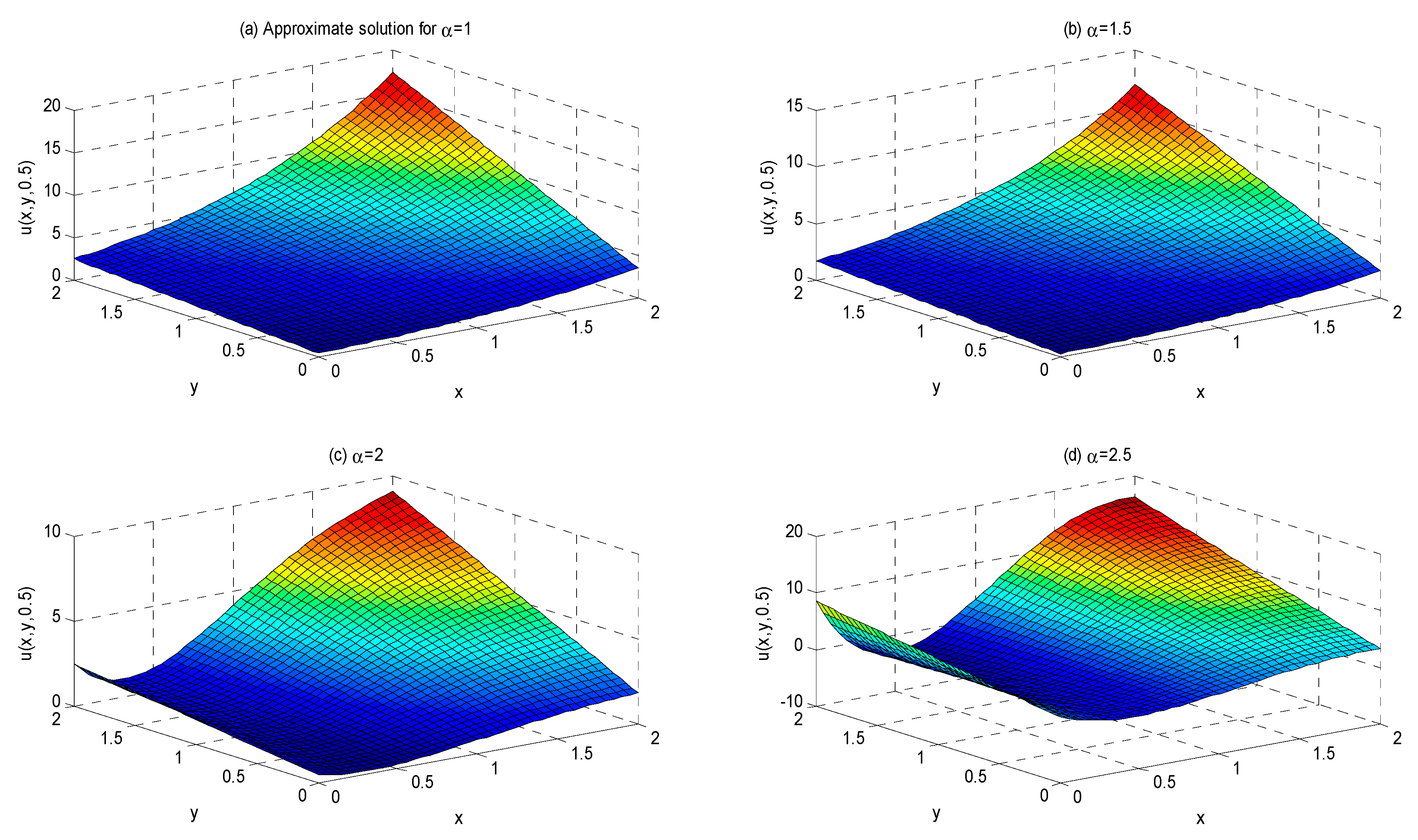
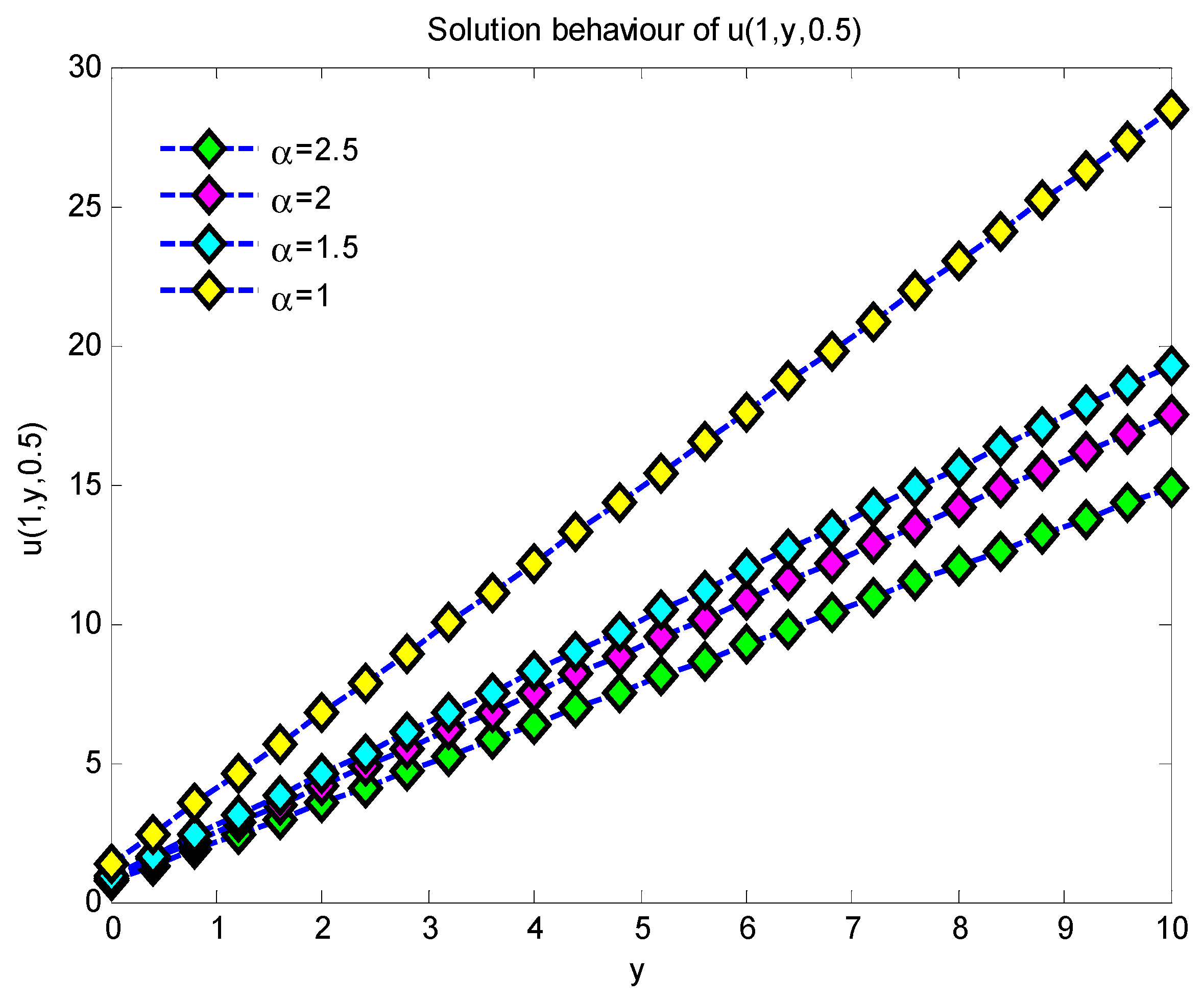
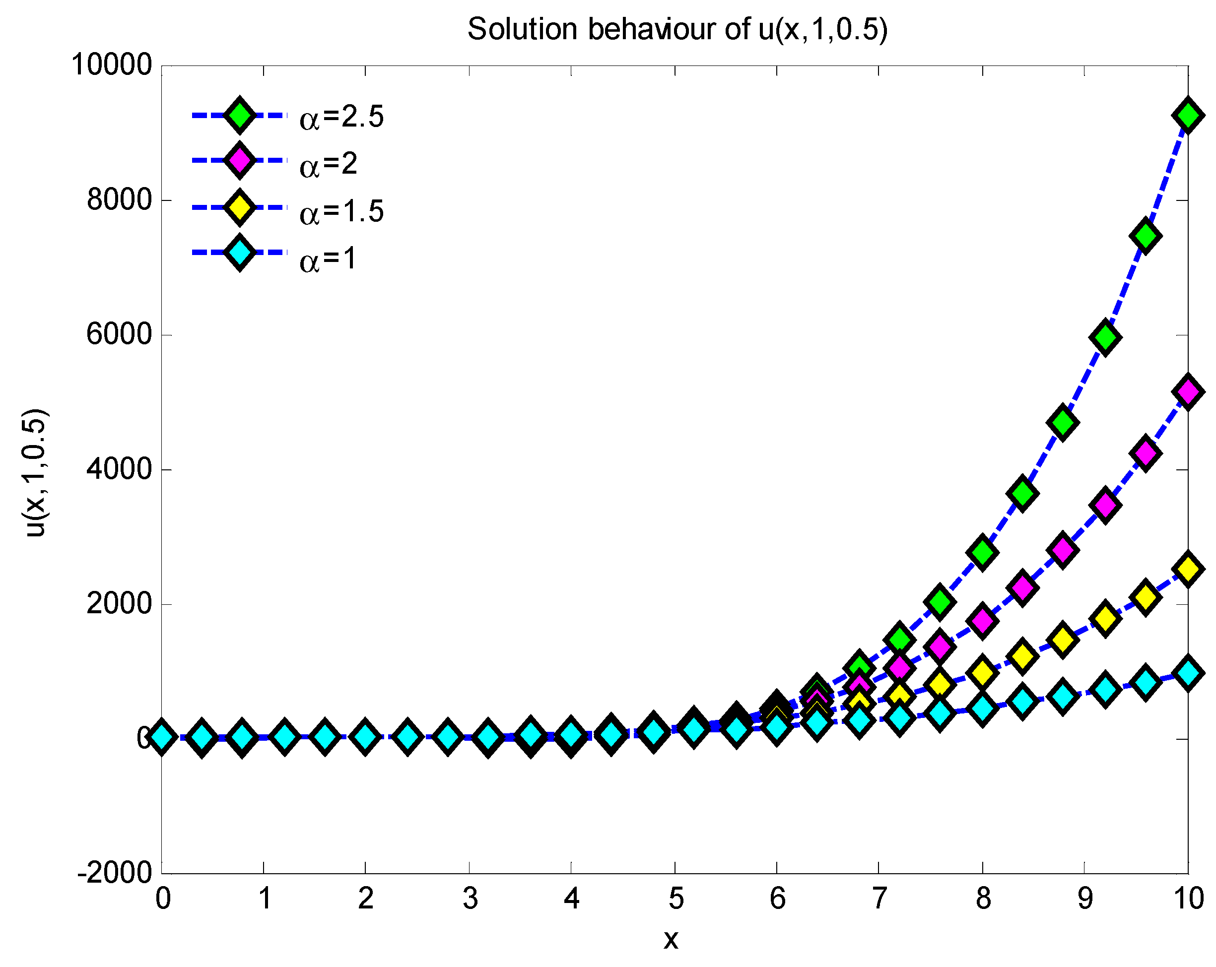
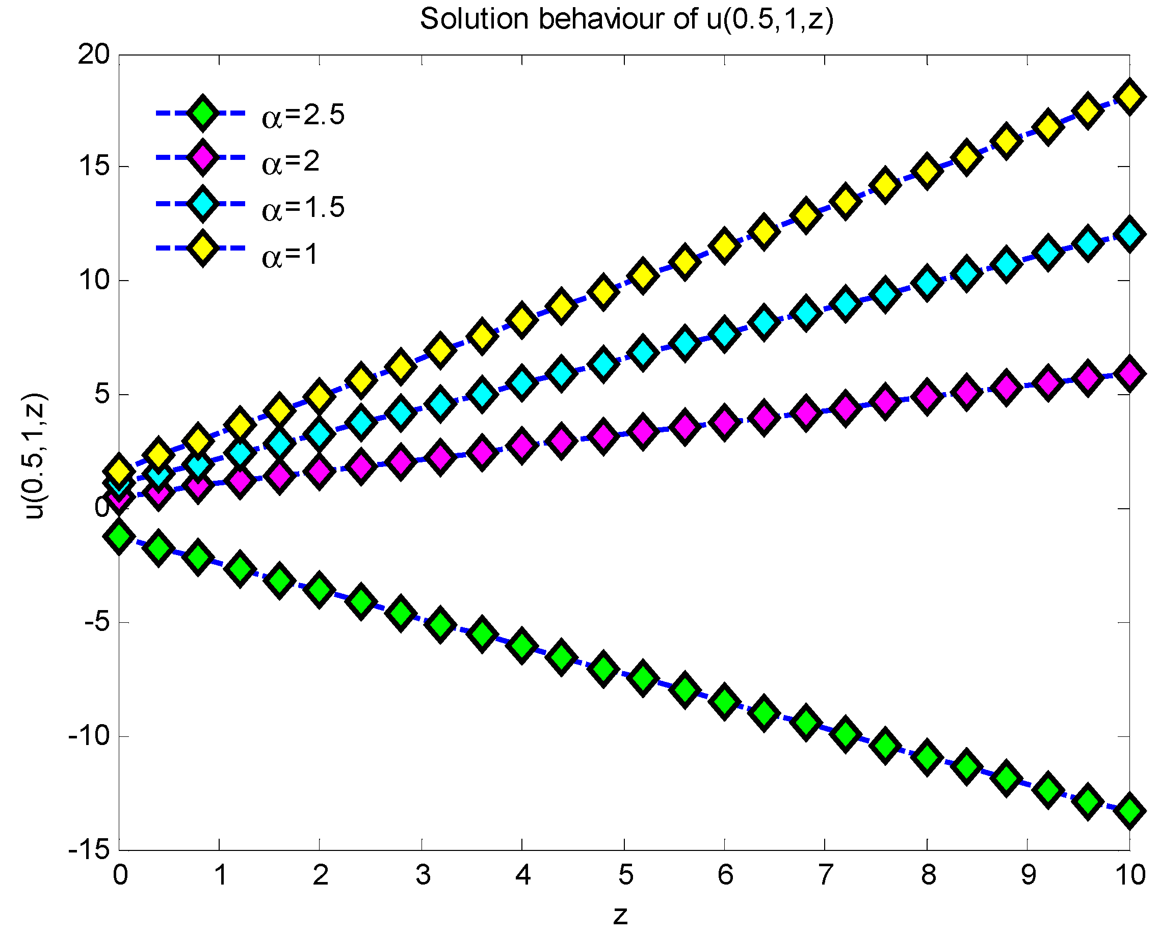
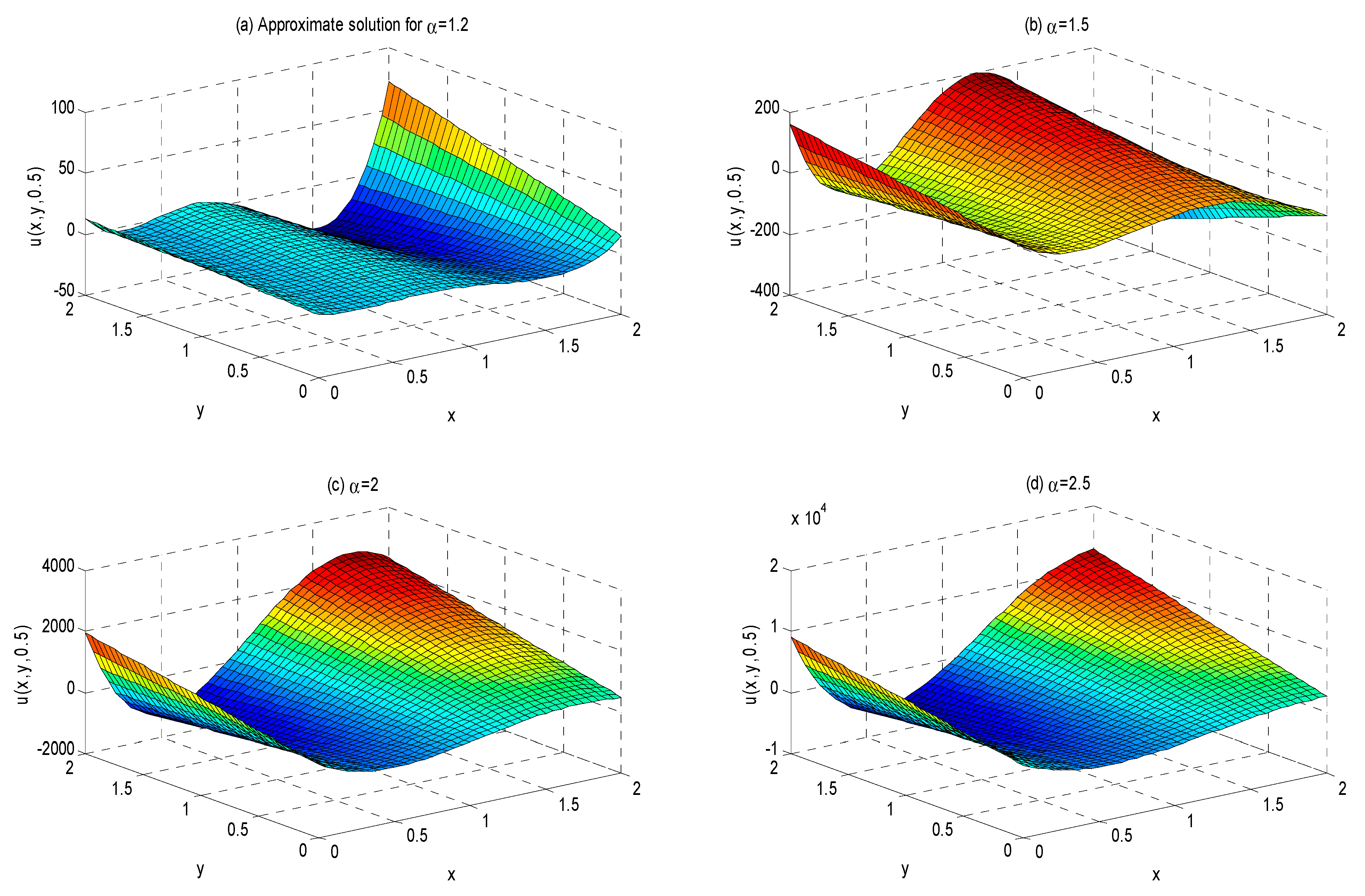
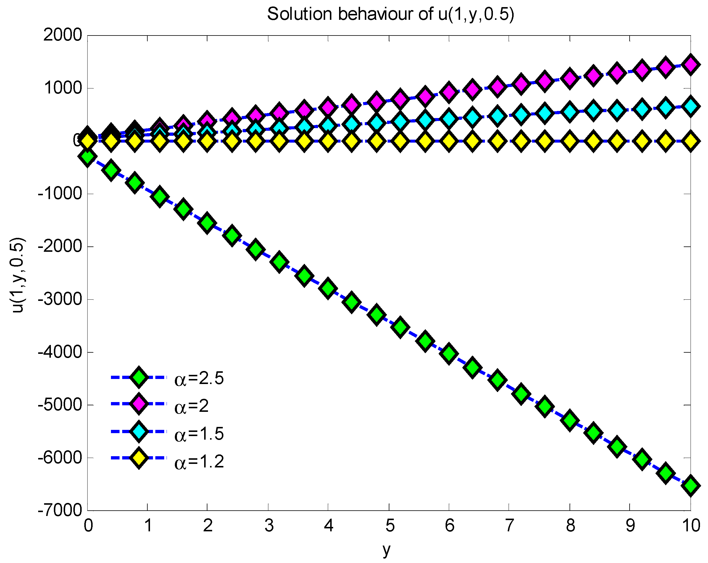
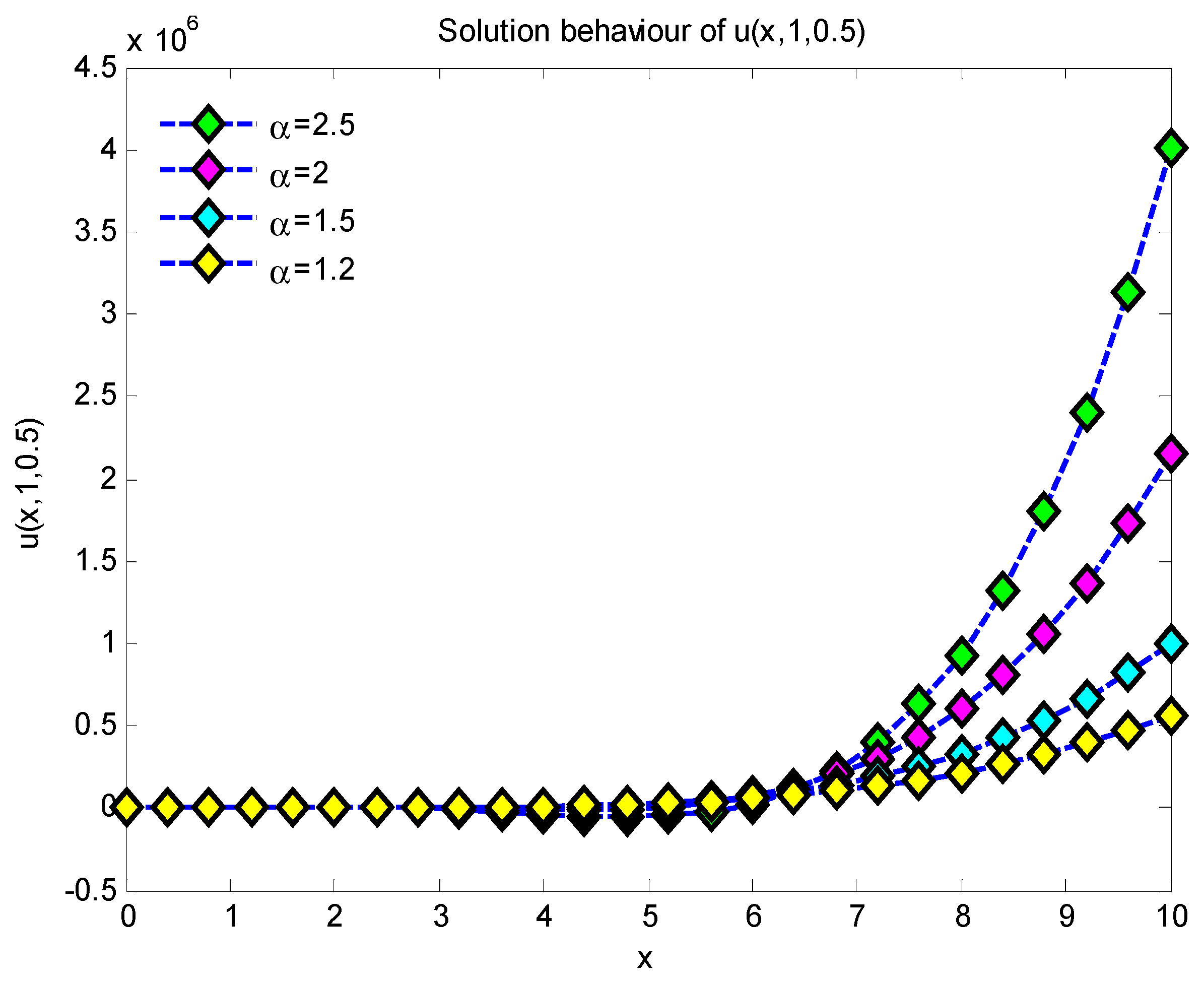
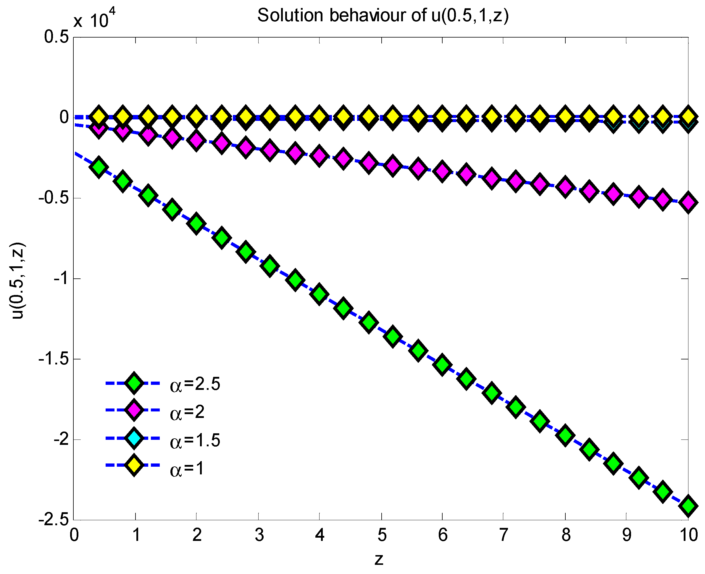
6. Results and Discussions

This work presents approximate analytical solutions demonstrating that the simulation results derived from the suggested approach closely align with the precise solution for fractional-order Helmholtz equations. Figure 1 illustrates the characteristics of the 3D plots representing the approximate precise solution of Example 1, where $0 \le x \le 2$ and $0 \le y \le 2$ for $u(x,y,0.5)$ with $\alpha$ values of 1, 1.5, 2, and 2.5. Figure 2 illustrates the characteristics of the 2D plots representing the approximate precise solution of Example 1 for $\alpha$ values of 1, 1.5, 2, and 2.5 throughout the range $0\le y\le 10$ for $u(1,y,0.5)$. As the value of $\alpha$ grows, the quantity of $u(1, y,0.5)$ solutions diminishes. The 2D plots of the approximate exact solution of Example 1 for values of $=1, 1.5, 2, 2.5,$ $0\le x\le 10$, and $u(x,1,0.5)$ are depicted in Figure 3. As the value of $\alpha$ increases, the number of solutions of $u(x,1,0.5)$ increases. Figure 4 illustrates the 2D plots of the approximation precise solution of Example 1 for $\alpha =1, 1.5, 2, 2.5,$ $0\le z\le 10,$ and $u(0.5,1,z)$. Increasing the value of $\alpha$ reduces the number of $u(0.5,1,z)$ solutions. Figure 5 depicts the attributes of the 3D plots that indicate the approximate exact solution of Example 2, where $0 \le x < 2$ and $0 \le y \le 2$ for $u(x,y,0.5)$, with α values of 1.2, 1.5, 2, and 2.5. In Figure 6, when the values of $\alpha =1.2, 1.5,$2 increase, the solution $u(1,y,0.5)$ also increases, but when $\alpha =2.5$, it is seen that the solutions for $u(1,y,0.5$) decrease very rapidly throughout the range $0\le y\le 10$. Figure 7 illustrates the 2D plots of the approximation precise solution for Example 2, with α values of 1.2, 1.5, 2, and 2.5 across the interval $0\le x\le 10$, and for $u(x,1,0.5)$. As the amount of α increases, the amount of $u(x,1, 0.5)$ solutions also increases. Figure 8 depicts the two-dimensional plots of the approximated exact solution of Example 1 for α values of 1, 1.5, 2, and 2.5, within the range of $0\le z\le 10$, and $u(0.5,1,z)$. Augmenting the value of α diminishes the quantity of $u(0.5, 1, z)$ solutions. From the graphical solutions, we observe that the approximate solutions closely match the exact solutions at $\alpha = 1$.

7. Conclusions

In this study, we employ a hybrid approach known as ATDM to examine the multidimensional fractional-order Helmholtz problem with Caputo–Fabrizio derivation. The fixed-point theorem determines both the existence and uniqueness of the suggested strategy. We solve two types of fractional-order Helmholtz equations to show that the suggested approach is accurate and effective. The findings demonstrate how computationally dependable and accurate the suggested approach is.

We examine two sample variants of the fractional Helmholtz model and establish the existence and uniqueness of the solution through the application of the fixed-point theorem. Numerical simulations demonstrate that the approach yields extremely accurate and computationally efficient solutions, affirming its promise for wider applications in fractional partial differential equations.

References

1. Abuasad, S.; Moaddy, K.; Hashim, I. Analytical treatment of two-dimensional fractional Helmholtz equations. J. King Saud Univ. Sci. 2019, 31, 659–666. [Google Scholar] [CrossRef]
2. Ghaffar, F.; Badshah, N.; Islam, S. Multigrid method for solution of 3d helmholtz equation based on hoc schemes. Abstr. Appl. Anal. 2014, 14, 954658. [Google Scholar] [CrossRef]
3. Gupta, P.K.; Yildirim, A.; Rai, K. Application of he’s homotopy perturbation method for multi-dimensional fractional helmholtz equation. Int. J. Numer. Methods Heat Fluid Flow 2012, 22, 424–435. [Google Scholar] [CrossRef]
4. Li, W. A fast singular boundary method for 3d helmholtz equation. Comp. Math. Appl. 2019, 77, 525–535. [Google Scholar] [CrossRef]
5. Li, J.; Chen, W.; Fu, Z.; Qin, Q.-A. A regularized approach evaluating the near-boundary and boundary solutions for three-dimensional helmholtz equation with wideband wave-Numbers. Appl. Math. Lett. 2019, 91, 55–60. [Google Scholar] [CrossRef]
6. Bespalov, A.; Betcke, T.; Haberl, A.; Praetorius, D. Adaptive bem with optimal convergence rates for the helmholtz equation. Comput. Methods Appl. Mech. Eng. 2019, 346, 260–287. [Google Scholar] [CrossRef]
7. Wang, K.; Wong, Y.S.; Deng, J. Efficient and accurate numerical solutions for helmholtz equation in polar and spherical coordinates. Commun. Comp. Phys. 2015, 17, 779–807. [Google Scholar] [CrossRef]
8. Qu, W.; Chen, W.; Gu, Y. Fast multipole accelerated singular boundary method for the 3d helmholtz equation in low frequency regime. Comp. Math. Appl. 2015, 70, 679–690. [Google Scholar] [CrossRef]
9. Alshammari, S.; Abuasad, S. Exact Solutions of the 3D Fractional Helmholtz Equation by Fractional Differential Transform Method. J. Func. Spac. 2022, 2022, 374751. [Google Scholar] [CrossRef]
10. Nadeem, M.; Abu Arqub, O.; Iambor, L.F.; Hussien, M.; Ebraheem Alzahrani, E. The Prospective Analysis of Three-Dimensional Time-Fractional Helmholtz Model using a New İterative Method. Fractals 2025, 33, 1–12. [Google Scholar] [CrossRef]
11. Nadeem, M.; Sharaf, M.; Mahamad, S. Numerical investigation of two-dimensional fractional Helmholtz equation using Aboodh transform scheme. Int. J. Heat Fluid Flow 2024, 34, 4520–4534. [Google Scholar] [CrossRef]
12. Shah, N.A.; El-Zahar, E.R.; Aljoufi, M.D.; Chung, J.D. An efficient approach for solution of fractional-order Helmholtz equations. Adv. Differ. Equ. 2021, 1, 14. [Google Scholar] [CrossRef]
13. Caputo, M.; Fabrizio, M. A New Definition of Fractional Derivative without Singular Kernel. Prog. Fract. Differ. Appl. 2015, 2, 73–85. [Google Scholar]
14. Losada, J.; Nieto, J.J. Properties of a New Fractional Derivative without Singular Kernel. Prog. Fract. Differ. Appl. 2015, 2, 87–92. [Google Scholar]
15. Atangana, A.; Baleanu, D. New Fractional Derivatives with Nonlocal and Non-Singular Kernel. Therm. Sci. 2016, 20, 763–769. [Google Scholar] [CrossRef]
16. Oprzędkiewicz, K.; Mitkowski, W.; Gawin, E.; Dziedzic, K. The Caputo vs. Caputo-Fabrizio operators in modeling of heat transfer process. Bull. Pol. Acad. Sci. Tech. Sci. 2018, 66, 4. [Google Scholar]
17. Aboodh, K.S. The New Integral Transform Aboodh Transform. Glob. J. Pure Appl. Math. 2013, 1, 35–43. [Google Scholar]
18. Aboodh, K.S. Application of New Transform Aboodh Transform to Partial Differential Equations. Glob. J. Pure Appl. Math. 2014, 2, 249–254. [Google Scholar]
19. Benattia, M.E.; Belghaba, K. Application of The Aboodh Transform for Solving Fractional Delay Differential Equations. Univ. J. Math. Appl. 2020, 3, 93–101. [Google Scholar] [CrossRef]
20. Şahin, Y.; Merdan, M.; Açıkgöz, P. The Novel Numerical Solutions for Caputo-Fabrizio Fractional Newell–Whitehead–Segel Equation by Using Aboodh-ADM. Res. Sq. 2024. [Google Scholar] [CrossRef]
21. Yasmin, H. Application of Aboodh Homotopy Perturbation Transform Method for Fractional-Order Convection–Reaction–Diffusion Equation within Caputo and Atangana–Baleanu Operators. Symmetry 2023, 15, 453. [Google Scholar] [CrossRef]
22. Alshehry, A.S.; Yasmin, H.; Shah, R.; Ali, A.; Khan, I. Fractional-order view analysis of Fisher’s and foam drainage equations within Aboodh transform. Eng. Comput. 2024, 41, 489–515. [Google Scholar] [CrossRef]
23. Iqbal, N.; Hussain, S.; Hamza, A.E.; Abdullah, A.; Mohammed, W.W.; Yar, M. Fractional dynamics study: Analytical solutions of modified Kordeweg-de Vries equation and coupled Burger’s equations using Aboodh transform. Sci. Rep. 2024, 14, 12751. [Google Scholar] [CrossRef] [PubMed]
24. Ojo, G.O.; Mahmudov, N.I. Aboodh Transform Iterative Method for Spatial Diffusion of a Biological Population with Fractional-Order. Mathematics 2021, 9, 155. [Google Scholar] [CrossRef]
25. Caputo, M.; Fabrizio, M. Applications of New Time and Spatial Fractional Derivatives with Exponential Kernels. Progr. Fract. Differ. Appl. 2016, 2, 1–11. [Google Scholar] [CrossRef]
26. Qureshi, S.; Rangaig, N.A.; Baleanu, D. New Numerical Aspects of Caputo-Fabrizio Fractional Derivative Operator. Mathematics 2019, 7, 374. [Google Scholar] [CrossRef]
27. Owolabi, K.M.; Atangana, A. Analysis and Application of New Fractional Adams–Bashforth Scheme With Caputo–Fabrizio Derivative. Chaos Solitons Fractal 2017, 109, 111–119. [Google Scholar] [CrossRef]
28. Al-Refai, M.; Pal, K. New Aspects of Caputo-Fabrizio Fractional Derivative. Progr. Fract. Differ. Appl. 2019, 5, 157–166. [Google Scholar] [CrossRef]
29. Bhangale, N.; Kachhia, K.; Gómez-Aguilar, J.F. A New Iterative Method with ρ Laplace Transform for Solving Fractional Differential Equations with Caputo Generalized Fractional Derivative. Eng. Comput. 2022, 38, 2125–2138. [Google Scholar] [CrossRef]
30. Mboro Nchama, G.A. Properties of Caputo-Fabrizio Fractional Operators. New Trends Math. Sci. 2020, 1, 1–25. [Google Scholar] [CrossRef]
31. Oyewumi, A.A.; Oderinu, R.A.; Ogunsola, A.W.; Taiwo, M.; Yahaya, A.A. A Numerical Solution of the Fractional Navier-Stokes Equation Using The Caputo-Fabrizio Aboodh Transform Method with the Reduced Differential Polynomials. Adv. Math. Sci. J. 2024, 13, 61–84. [Google Scholar] [CrossRef]
32. Ziane, D.; Belgacem, R.; Bokhari, A. A New Modified Adomian Decomposition Method for Nonlinear Partial Differential Equations. Open J. Math. Anal. 2019, 3, 81–90. [Google Scholar] [CrossRef]
33. Şahin, Y.; Merdan, M. The Solutions of Caputo-Fabrizio Random Fractional Ordinary Differential Equations by Aboodh Transform Method. Erzincan Üniversitesi Fen Bilim. Enstitüsü Derg. 2025, 18, 149–170. [Google Scholar] [CrossRef]
34. Şahin, Y. Solutions of Random Fractional Differential Equations Using Aboodh and Aboodh-Adomian Decomposition Method. Master’s Thesis, Gumushane University, Gümüşhane, Turkey, 2024. [Google Scholar]
35. Şahin, Y.; Merdan, M. New Numerical Solutions for Caputo–Fabrizio Fractional Differential Multidimensional Diffusion Problems. Int. J. Math. Mathemat. Sci. 2025, 1, 5554516. [Google Scholar] [CrossRef]
36. Bekela, A.S.; Deresse, A.T. A hybrid yang transform adomian decomposition method for solving time-fractional nonlinear partial differential equation. BMC Rese. Not. 2024, 17, 226. [Google Scholar] [CrossRef] [PubMed]
37. Veeresha, P.; Prakasha, D.G.; Baskonus, H.M. Solving smoking epidemic model of fractional order using a modified homotopy analysis transform method. Math. Sci. 2019, 13, 115–128. [Google Scholar] [CrossRef]
38. Kumar, D.; Singh, J.; Baleanu, D. A new analysis for fractional model of regularized long-wave equation arising in ionacoustic plasma waves. Math. Methods Appl. Sci. 2017, 40, 5642–5653. [Google Scholar] [CrossRef]
39. Magreñán, Á.A. A new tool to study real dynamics: The convergence plane. Appl. Math. Comput. 2014, 248, 215–224. [Google Scholar] [CrossRef]
40. Kırane, M.; Turmetovand, B.K.H.; Torebek, T.B. A Nonlocal Fractional Helmholtz Equation. Fract. Differ. Calc. 2017, 7, 225–234. [Google Scholar] [CrossRef]
41. Khan, A.; Liaqat, M.İ.; Mushtaq, A. Analytical Analysis for Space Fractional Helmholtz Equations by Using the Hybrid Efficient Approach. Acta Mech. Autom. 2024, 18, 4. [Google Scholar] [CrossRef]
42. Juraev, D.A.; Agarwal, P.; Elsayed, E.E.; Targyn, N. Helmholtz Equations and Their Applications in Solving Physical Problems. Adv. Eng. Sci. 2024, 4, 54–64. [Google Scholar]
43. Alesemi, M.; Iqbal, N.; Wyal, N. Novel Evaluation of Fuzzy Fractional Helmholtz Equations. J. Funct. Spaces 2022, 2022, 8165019. [Google Scholar] [CrossRef]
44. Wang, K. New computational approaches to the fractional coupled nonlinear Helmholtz equation. Eng. Comput. 2024, 41, 1285–1300. [Google Scholar] [CrossRef]
45. Nadeem, M.; Li, Z.; Kumar, D.; Alsayaad, Y. A Robust Approach for Computing Solutions of Fractional-Order two-Dimensional Helmholtz Equation. Sci. Rep. 2024, 14, 4152. [Google Scholar] [CrossRef] [PubMed]
46. Hoana, L.V.C.; Korpinar, Z.; Inc, M.; Chue, Y.-M.; Almohseng, B. On Convergence Analysis and Numerical Solutions of Local Fractional Helmholtz Equation. Alex. Eng. J. 2020, 59, 4335–4341. [Google Scholar] [CrossRef]
47. Samuel, M.S.; Thomas, A. On Fractional Helmholtz Equations. Fract. Calc. Appl. Anal. 2010, 13, 295–308. [Google Scholar]
48. Baleanu, D.; Jassim, H.K.; Al Qurash, M. Solving Helmholtz Equation with Local Fractional Derivative Operators. Fractal Fract. 2019, 3, 43. [Google Scholar] [CrossRef]
49. Srivastava, H.M.; Shah, R.; Khan, H.; Arif, M. Some analytical and numerical investigation of a family of fractional-order Helmholtz equations in two space dimensions. Math. Meth. Appl. Sci. 2020, 1, 199–212. [Google Scholar] [CrossRef]
Figure 1. The 3D visual structure with different value of α when 0 x 2 , 0 y 2 , and t = 0.5 .
Symmetry 17 01219 g001
Figure 2. Two-dimensional solution behavior of u ( 1 , y , 0.5 ) for α = 2.5 ,   2 ,   1.5 , and 1 .
Symmetry 17 01219 g002
Figure 3. Two-dimensional solution behavior of u ( x , 1 , 0.5 ) for α = 2.5 ,   2 ,   1.5 , and 1 .
Symmetry 17 01219 g003
Figure 4. Two-dimensional solution behavior of u ( 0.5 , 1 , z ) for α = 2.5 ,   2 ,   1.5 , and 1 .
Symmetry 17 01219 g004
Figure 5. The 3D visual structure with different value of α = 1.2 ,   1.5 ,   2 ,   2.5 when 0 x 2 , 0 y 2 , and t = 0.5 .
Symmetry 17 01219 g005
Figure 6. Two-dimensional solution behavior of u ( 1 , y , 0.5 ) for α = 2.5 ,   2 ,   1.5 , and 1.2 .
Symmetry 17 01219 g006
Figure 7. Two-dimensional solution behavior of u ( x , 1 , 0.5 ) for α = 2.5 ,   2 ,   1.5 , and 1.2 .
Symmetry 17 01219 g007
Figure 8. Two-dimensional solution behavior of u ( 0.5 , 1 , z ) for α = 2.5 ,   2 ,   1.5 , and 1.
Symmetry 17 01219 g008
Disclaimer/Publisher’s Note: The statements, opinions and data contained in all publications are solely those of the individual author(s) and contributor(s) and not of MDPI and/or the editor(s). MDPI and/or the editor(s) disclaim responsibility for any injury to people or property resulting from any ideas, methods, instructions or products referred to in the content.