Adaptive Learning Control for Vehicle Systems with an Asymmetric Control Gain Matrix and Non-Uniform Trial Lengths

Abstract

Intelligent driving is a key technology in the field of automotive manufacturing due to its advantages in environmental protection, energy efficiency, and economy. However, since the intelligent driving model is an uncertain multi-input multi-output dynamic system, especially in an interactive environment, it faces uncertainties such as non-uniform trial lengths, unknown nonlinear parameters, and unknown control direction. In this paper, an adaptive iterative learning control method is proposed for vehicle systems with non-uniform trial lengths and asymmetric control gain matrices. Unlike the existing research on adaptive iterative learning for non-uniform test lengths, this paper assumes that the elements of the system’s control gain matrix are asymmetric. Therefore, the assumption made in traditional adaptive iterative learning methods that the control gain matrix of the system is known or real, symmetric, and positive definite (or negative definite) is relaxed. Finally, to prove the convergence of the system, a composite energy function is designed, and the effectiveness of the adaptive iterative learning method is verified using vehicle systems. This paper aims to address the challenges in intelligent driving control and decision-making caused by environmental and system uncertainties and provides a theoretical basis and technical support for intelligent driving, promoting the high-quality development of intelligent transportation.

1. Introduction

As an important component of future transportation systems, intelligent driving has significant development advantages. In the actual operation of intelligent driving vehicles [1,2,3,4], tracking task repetition is one of the common tasks. This repetition typically involves the repeated driving of vehicles along specific paths or trajectories, and it occurs in fixed-route buses, logistics delivery vehicles, park shuttle buses, port container transportation, airport baggage transportation, and factory material transportation. These operations are usually highly regular and predictable, making them well-suited for automated processing by intelligent driving systems. By continuously optimizing path-tracking algorithms and control strategies, intelligent driving vehicles can achieve efficient and safe operation in these scenarios.

For trajectory-tracking tasks that are repeated within a finite time interval, which is different to asymptotic tracking over infinite time [5,6,7,8,9,10,11,12,13,14,15,16,17,18], iterative learning control [19,20,21,22,23,24,25,26] is an effective control strategy which performs the same task repeatedly over a finite time interval. The core idea is to improve tracking performance from one execution (called a “trial”, “pass”, or “iteration”) to the next by utilizing data (like tracking errors and control signals) from previous executions, leveraging past control experience to enhance the current tracking performance of dynamic systems. For example, iterative learning control effectively addresses the challenges of repetitive operations for underwater robots in complex hydrodynamic environments such as subsea pipeline inspection systems and underwater equipment maintenance scenarios. These applications have promoted the proposal of iterative learning control methods. Wei et al. proposed an iterative learning control (ILC) approach for nonlinear systems with iteratively varying reference trajectories and random initial state shifts, and established theoretical proofs of error convergence [26]. The advantage of the iterative learning control method is that it does not require a precisely known system model, the controller structure is simple, and it is suitable for controlled systems with high tracking accuracy requirements, strong coupling, or complex nonlinearity. In the past three decades, significant progress has been made in iterative learning control in both basic theory and experimental applications [23,24,25,26].

However, most existing iterative learning control designs require that the system object, initial state, reference trajectory, and test length in the iterative learning control process remain constant as the number of iterations increases [22], especially for processing the same test length [26,27]. In fact, it is difficult to repeatedly perform the same task within a fixed time interval in practice. For example, during underwater robotic seabed inspections, when the multimodal sensor array detects deviations in critical hydroacoustic signal characteristics beyond preset thresholds, the system activates failure determination protocols, terminates the current operation, and autonomously transitions to the next inspection target. Another example is in the field of fully automated precision manufacturing, where semi-finished products undergo a series of processing steps to ultimately form highly integrated end products. This method intertwines the processing and inspection stages in a complex manner; any defect in the processing operation can jeopardize the success of the entire production line, and detecting irreparable faults in semi-finished products during the inspection phase can lead to automatic stoppage of the manufacturing process. Therefore, non-uniform trial lengths are quite common in real life. For non-uniform trial lengths, the average operator technique and modified tracking error are used to provide corresponding iterative learning control algorithms [28,29], and the robustness and convergence of iterative learning control errors are analyzed using constant norms. On the other hand, most of the research has focused on discrete-time linear systems [30,31], mainly due to the beneficial system structure and mature discrete random variable analysis techniques. Although for nonlinear systems [32], the nonlinear function involved needs to satisfy the global Lipschitz condition.

In the past few decades, by introducing the concept of adaptive control into the design of iterative learning control, an important class of iterative learning control algorithms has been proposed, known as adaptive iterative learning control methods [33,34,35]. The main features of such methods are the estimation of uncertain control parameters between successive iterations and the use of these parameters to generate the current control input. Adaptive iterative learning control is a control method applied to dynamic systems in continuous or discrete time. It combines the ideas of adaptive control and iterative learning control methods and gradually improves the control performance of the system through learning during the iterative process. In the adaptive iterative learning control method, the controller adjusts according to the error between the real-time response of the system and the desired output. Through continuous iteration, the controller can gradually learn the dynamic characteristics of the system and improve the control strategy based on the learned knowledge, thereby achieving better control performance. Adaptive iterative learning control methods are typically employed for underwater robots performing repetitive operational tasks in complex hydrodynamic environments, such as subsea trajectory tracking or precision manipulation of seabed equipment. They can gradually reduce the tracking error of the system through multiple iterations and improve the stability and robustness of the system. In practical applications, adaptive iterative learning control methods need to consider factors such as the dynamic characteristics, learning speed, and convergence of the system. At the same time, selecting the appropriate learning algorithm and control strategy is also a crucial step. Adaptive iterative learning control methods have obvious advantages in relaxing the global Lipschitz continuity condition, handling non-uniform initial states, iteratively changing reference trajectories, and dealing with external disturbances. Liu et al. studied the problem of variable test length for continuous-time nonlinear systems based on adaptive iterative learning control methods [33]. However, their system was a single-input single-output system, and the input gain or control direction was a scalar value. An adaptive iterative learning method was proposed to solve the problem of random changes in the length of the experiment. However, the system involved in the study involved multiple input and multiple output systems [34]. The system was parameterized, and the control gain matrix of the system was assumed to be known.

In fact, the control gain matrix in a multi-input multi-output system [36,37,38] is the derivative of the system output to the control input, and it is usually required to be symmetric and positive definite (or negative definite). However, in most underwater robotic propulsion systems (e.g., multi-thruster power distribution systems [36] and articulated drive systems [37]), the control gain matrices consistently exhibit off-diagonal coupling characteristics, which constitutes a prominent system feature arising from hydrodynamic anisotropy. Obviously, the assumption of the positive (or negative) definiteness of the control gain matrix, or even the assumption of knownness, greatly limits the development of adaptive iterative learning control.

This paper proposes a new adaptive iterative control strategy for multi-input multi-output nonlinear vehicle systems with non-uniform test lengths and asymmetric control gain matrices, which relaxes the assumption requirements that stipulate that the traditional control gain matrices are positive definite (or negative definite) or even known. The key features and contributions of the paper are as follows:

• Vehicle systems for intelligent driving are investigated for reference trajectory tracking in an infinite iteration domain with non-uniform trial lengths.
• In the adaptive control community, it is generally required that the control gain matrices of plants be real, symmetric, and positive definite (or negative definite), but, in this paper, only the asymmetric control gain matrices in the vehicle systems are assumed.
• Unlike those fuzzy systems or neural network-based techniques used for adaptive iterative learning control, less adaptive variables are designed for adjusting or updating in the proposed method such that the structure of the controller is very simple and the memory space for computing is greatly saved.

2. Problem Formulation

2.1. Intelligent Driving Vehicle System

This paper focuses on an in-depth study of a control system for intelligent driving vehicles in interactive environments. In real-world traffic scenarios, intelligent driving vehicles do not operate in isolation but constantly interact with other traffic participants, such as other vehicles and pedestrians. This interaction has a crucial impact on the safety and efficiency of intelligent driving vehicles. Therefore, constructing an accurate and reasonable dynamic model of the control system is a key foundation for achieving safe and efficient intelligent driving. Consider the following dynamic model of a control system for intelligent driving vehicles in an interactive environment that moves within a finite time interval:

$${\dot{\mathbf{x}}}_{p,k}\left(t\right)=g({\mathbf{x}}_{p,k}\left(t\right),t)+\mathbf{G}{\mathbf{u}}_{p,k}\left(t\right)+{\mathbf{A}}_{p,q}{\mathbf{x}}_{q,k}\left(t\right),t\in [0,T]$$

(1)

Here, k represents the system iteration number. During the system optimization and parameter adjustment process, the accuracy and adaptability of the model are continuously improved through multiple iterations. $t\in [0,T]$ represents continuous time, where T is the set upper limit of the finite time, covering the time period of vehicle motion analysis that we are concerned about. ${\mathbf{x}}_{p,k}\left(t\right)\in {\mathbb{R}}^l$ is the state vector of the p-th vehicle at the k-th iteration and time t. This vector usually includes key state variables such as the vehicle’s position, velocity, and acceleration, comprehensively describing the vehicle’s motion state in space. ${\mathbf{x}}_{q,k}\left(t\right)\in {\mathbb{R}}^l$ is the state vector of the q-th vehicle at the corresponding time and iteration number, also recording various motion information of this vehicle. ${\mathbf{u}}_{p,k}\left(t\right)\in {\mathbb{R}}^l$ is the control input vector of the p-th vehicle. For example, control commands such as the steering wheel angle, accelerator pedal opening, and braking force are used to adjust the vehicle’s operating state. $\mathbf{G}\in {\mathbb{R}}^{l\times l}$ is the control gain matrix. It not only determines the direction of the effect of the control input on the system output but also, essentially, represents the derivative of the system output with respect to the control input, reflecting the sensitivity of the vehicle state change to the control commands. However, in practical applications, $\mathbf{G}$ is unknown, its values are bounded, and it is non-symmetric, which poses challenges for the design of the control system. $g({\mathbf{x}}_{p,k}\left(t\right),t)\in {\mathbb{R}}^l$ is the unknown nonlinear vector function of vehicle p itself, used to describe the parts of the vehicle’s own motion characteristics that cannot be expressed by linear relationships, such as the changes in the vehicle’s dynamic characteristics when driving on complex road surfaces.

In an interactive environment, to accurately depict the interactions between vehicles, it is necessary to determine the interaction relationships according to the behavioral characteristics of traffic participants. Taking vehicle-to-vehicle interactions as an example, the influence of vehicle p on vehicle q may be reflected in many aspects. Common ones include car-following behavior: vehicle p adjusts its own speed according to the speed and distance of the preceding vehicle q to maintain a safe following distance; evasion behavior: when vehicle p detects that vehicle q may pose a collision risk, it actively changes its driving direction or speed to avoid the collision; and path adjustment: vehicle p may re-plan its driving route due to the influence of vehicle q’s driving path on its own planned path.

Based on the characteristics of these interaction relationships, further quantifying the interaction intensity is an important part of constructing an accurate model. In the quantification process, various indicators can be used. For example, physical quantities such as distance, speed difference, and acceleration difference are used to measure the degree of interaction between vehicles. At the same time, in order to reflect the differences in the importance of different state variables during the interaction process, weight coefficients are introduced to represent the influence degree of different state variables. Finally, the quantified interaction intensity is represented in matrix form as follows:

$${\mathbf{A}}_{p,q}=\left[\begin{array}{cccc}{a}_{11}& a_{12}& \dots & a_{1l}\\ a_{21}& a_{22}& \dots & a_{2l}\\ ⋮& ⋮& \ddots & ⋮\\ a_{l1}& a_{l2}& \dots & a_{ll}\end{array}\right]$$

The element $a_{ij}$ in the matrix ${\mathbf{A}}_{p,q}$ represents the influence weight of the j-th state variable of the q-th vehicle on the i-th state variable of the p-th vehicle. The entire matrix ${\mathbf{A}}_{p,q}$ comprehensively describes the influence of vehicle q on vehicle p.

Assumption 1. 

Let the nonlinear mapping $g({\mathbf{x}}_{p,k}\left(t\right),t)$ satisfy the sublinear growth constraint as follows:

$${∥g({\mathbf{x}}_{p,k}\left(t\right),t)∥}_{\infty }\le {\alpha }_1{∥{\mathbf{x}}_{p,k}\left(t\right)∥}_{\infty }+{\alpha }_2,$$

where ${\alpha }_1$ and ${\alpha }_2$ denote positive-definite parameters.

Assumption 2. 

The iterative learning process satisfies the uniform boundedness conditions: all iterative initial values ${\mathbf{x}}_{p,k}\left(0\right)\in R^n$, expected trajectories are ${\mathbf{r}}_d\left(t\right)$ iterative transformations, external disturbances ${\mathbf{w}}_k\left(t\right)={\mathbf{A}}_{p,q}{\mathbf{x}}_{q,k}\left(t\right)$, and ${\mathbf{x}}_{p,k}\left(0\right)={\mathbf{r}}_d\left(0\right)$.

Assumption 1 is often used in iterative learning control designs for nonlinear dynamic systems and practical applications. Assumption 2 is a common constraint condition and is reasonable in practical physical systems. In fact, if the nonlinear function of a system changes too rapidly or the initial value of the system is unbounded, it is obvious that it will not meet the requirements of an actual system.

2.2. Design of Adaptive Iterative Learning Controller for Non-Uniform Test Length

2.2.1. Non-Uniform Trial Length

In conventional iterative learning control (ILC) algorithms, the task execution time interval is strictly confined to a fixed duration to facilitate an idealized iterative learning process. However, in practical applications, this requirement frequently becomes infeasible due to inherent uncertainties and unpredictable disturbances. This fundamental challenge has motivated substantial research addressing uneven trial lengths. The following representative scenarios exemplify typical manifestations of non-uniform trial durations in real-world implementations.

As a foundational step in constructing the adaptive iterative learning control (AILC) framework, the system’s tracking error must be formally defined:

$$E_k\left(t\right)={\mathbf{r}}_d\left(t\right)-{\mathbf{x}}_{p,k}\left(t\right),$$

(2)

where ${\mathbf{r}}_d\left(t\right)$ represents the desired trajectory and $E_k\left(t\right)=\left[\begin{array}{cccc}{E}_k^{\left(1\right)}\left(t\right)& E_k^{\left(2\right)}\left(t\right)& \dots & E_k^{\left(n\right)}\left(t\right)\end{array}\right]$.

Under non-uniform trial length conditions, ${\tau }_k$ denotes the duration of each iterative operation. The modified tracking error is formulated as follows:

$${\mathbf{f}}_k\left(t\right)=\left\{\begin{array}{cc}{E}_k\left(t\right),\hfill & 0\le t\le {\tau }_k\hfill \\ E_k\left({\tau }_k\right),\hfill & {\tau }_k<t\le T\hfill \end{array}\right.$$

It can be concluded that ${\mathbf{f}}_k\left(t\right)={\lambda }_k{E}_k\left(t\right)+(1-{\lambda }_k)E_k\left({\tau }_k\right)$, where ${\lambda }_k\in \{0,1\}$. When ${\lambda }_k=1$, the system stops halfway during task execution and fails to reach the desired trial duration; conversely, when ${\lambda }_k=0$, the system reaches the desired duration.

2.2.2. Controller Design

Building upon Assumptions 1–3 as the theoretical foundation, this study develops an adaptive iterative learning control scheme with the following architectural configuration:

$${\mathbf{u}}_{p,k}\left(t\right)={\displaystyle \frac{\widehat{\mathbf{G}}{E}_k\left(t\right)E_k^T\left(t\right)\xi \left(E_k\left(t\right)\right){ϵ}_k\left(t\right)}{\parallel E_k{\left(t\right)\parallel }_2^2}}$$

(3)

$${\widehat{ϵ}}_k\left(t\right)=\left\{\begin{array}{cc}{\widehat{ϵ}}_{k-1}\left(t\right)+\Gamma {\xi }^T\left(E_k\left(t\right)\right)E_k\left(t\right)\in R^2,& 0\le t\le {\tau }_k\\ {\widehat{ϵ}}_{k-1}\left(t\right)\in R^2,& {\tau }_k<t\le T\end{array}\right.$$

(4)

$$\xi \left(E_k\left(t\right)\right)=\left[\begin{array}{cc}{E}_k\left(t\right)& \mathrm{sign}\left(E_k\left(t\right)\right)\end{array}\right]\in R^{n\times 2},$$

(5)

where ${\widehat{ϵ}}_{-1}\left(t\right)=0\in R^2$, and $\Gamma \in R^n$ is the learning gain to be designed. Equation (3) formulates the control input that constitutes the core controller architecture, while Equation (4) defines the adaptive parameter-updating mechanism. The algorithm’s innovation resides in its synergistic optimization process, which integrates cross-iteration parameter transfer with error feedback, dynamically calibrating control parameters through historical iteration data and real-time error signals to achieve progressive input refinement.

2.2.3. Stability Analysis

Theorem 1. 

Based on Assumptions 1 and 2, under the action of the adaptive control law (3) and adaptive parameter update laws (4) and (5), when the control gain matrix $\mathbf{G}$ of the vehicle system satisfies $\sigma (-\mathbf{G}\widehat{\mathbf{G}})\subset C^{-}$ and $\Gamma >0$ is satisfied, the tracking error of the system is ${lim}_{k\to \infty }{E}_k\left(t\right)=0$.

Proof. 

Because of $\sigma (-\mathbf{G}\widehat{\mathbf{G}})\subset C^{-}$, there exists a positive-definite symmetric matrix $Q=Q^T\in R^{n\times n}$ satisfying

$${\left(\mathbf{G}\widehat{\mathbf{G}}\right)}^{T}Q+Q\left(\mathbf{G}\widehat{\mathbf{G}}\right)=2I_n.$$

(6)

Building upon the theoretical foundation of Assumptions 1 and 2, we establish the following formal definition:

$$\underset{0\le t\le T}{\sup }{∥Q{\dot{\mathbf{r}}}_d\left(t\right)-Q{\mathbf{w}}_k\left(t\right)∥}_{\infty }\le \alpha$$

(7)

$$\underset{0\le t\le T}{\sup }{∥Q∥}_{m_{\infty }}\le c,$$

(8)

and

$$\left\{\begin{array}{c}h=nc{\alpha }_1\\ j=n\alpha +nc{\alpha }_1{∥{\mathbf{r}}_d\left(t\right)∥}_{\infty }+nc{\alpha }_2\end{array}\right.$$

(9)

$$ϵ={\left[\begin{array}{cc}h& j\end{array}\right]}^T\in R^2,$$

(10)

A composite-type energy function is formulated as follows:

$$V_k\left(t\right)={\displaystyle \frac{1}{2}}{{\mathbf{f}}_k}^T\left(t\right)Q{\mathbf{f}}_k\left(t\right)+{\displaystyle \frac{1}{2}}{\int }_0^t{\widetilde{ϵ}}_k^T\left(t\right){\Gamma }^{-1}{\widetilde{ϵ}}_k\left(t\right)\mathrm{d}\tau$$

(11)

where the estimated error of $ϵ$ is ${\widetilde{ϵ}}_k\left(t\right)=ϵ-{\widehat{ϵ}}_k\left(t\right)$, and ${\widehat{ϵ}}_k\left(t\right)$ is the estimated value of $ϵ$.

Step 1: To prove that sequence $\left\{V_k\left(t\right)\right\}$ is a monotone non-increasing sequence, the difference in $V_k\left(t\right)$ is first defined in the iterative direction:

$$\begin{array}{cc}\hfill \Delta V_k\left(t\right)& =V_k\left(t\right)-V_{k-1}\left(t\right)\hfill \\ \hfill & ={\displaystyle \frac{1}{2}}{{\mathbf{f}}_k}^T\left(t\right)Q{\mathbf{f}}_k\left(t\right)-{\displaystyle \frac{1}{2}}{f_{k-1}}^T\left(t\right)Q{f}_{k-1}\left(t\right)+{\int }_0^t{\displaystyle \frac{1}{2}}\left({\widetilde{ϵ}}_k^T\left(\tau \right){\Gamma }^{-1}{\widetilde{ϵ}}_k\left(\tau \right)-{\widetilde{ϵ}}_{k-1}^T\left(\tau \right){\Gamma }^{-1}{\widetilde{ϵ}}_{k-1}\left(\tau \right)\right)\mathrm{d}\tau \hfill \end{array}$$

(12)

It can be observed that the difference in $V_k\left(t\right)$ consists of two parts: the error term and the adaptive parameter estimation error term.

When $0\le t\le {\tau }_k$, the adaptive parameter estimation error term for $V_k\left(t\right)$ yields the following result:

$$\begin{array}{cc}\hfill & {\displaystyle \frac{1}{2}}{\widetilde{ϵ}}_k^T\left(t\right){\Gamma }^{-1}{\widetilde{ϵ}}_k\left(t\right)-{\displaystyle \frac{1}{2}}{\widetilde{ϵ}}_{k-1}^T\left(t\right){\Gamma }^{-1}{\widetilde{ϵ}}_{k-1}\left(t\right)\hfill \\ \hfill & ={\displaystyle \frac{1}{2}}{\widetilde{ϵ}}_k^T\left(t\right){\Gamma }^{-1}{\widetilde{ϵ}}_k\left(t\right)+{\displaystyle \frac{1}{2}}{\widetilde{ϵ}}_k^T\left(t\right){\Gamma }^{-1}{\widetilde{ϵ}}_{k-1}\left(t\right)-{\displaystyle \frac{1}{2}}{\widetilde{ϵ}}_{k-1}^T\left(t\right){\Gamma }^{-1}{\widetilde{ϵ}}_k\left(t\right)-{\displaystyle \frac{1}{2}}{\widetilde{ϵ}}_{k-1}^T\left(t\right){\Gamma }^{-1}{\widetilde{ϵ}}_{k-1}\left(t\right)\hfill \\ \hfill & ={\displaystyle \frac{1}{2}}{\left({\widetilde{ϵ}}_k\left(t\right)-{\widetilde{ϵ}}_{k-1}\left(t\right)\right)}^T{\Gamma }^{-1}\left({\widetilde{ϵ}}_k\left(t\right)+{\widetilde{ϵ}}_{k-1}\left(t\right)\right)\hfill \\ \hfill & =-{\displaystyle \frac{1}{2}}{\left({\widehat{ϵ}}_k\left(t\right)-{\widehat{ϵ}}_{k-1}\left(t\right)\right)}^T{\Gamma }^{-1}\left(2{\widetilde{ϵ}}_k\left(t\right)+\left({\widehat{ϵ}}_k^T\left(t\right)-{\widehat{ϵ}}_{k-1}\left(t\right)\right)\right)\hfill \end{array}$$

(13)

By incorporating the adaptive parameter update mechanism into Equation (13) and performing integration on both sides, the following relationship is derived:

$$\begin{array}{cc}\hfill & {\int }_0^t{\displaystyle \frac{1}{2}}\left({\widetilde{ϵ}}_k^T\left(\tau \right){\Gamma }^{-1}{\widetilde{ϵ}}_k\left(\tau \right)-{\widetilde{ϵ}}_{k-1}^T\left(\tau \right){\Gamma }^{-1}{\widetilde{ϵ}}_{k-1}\left(\tau \right)\right)\mathrm{d}\tau \hfill \\ \hfill & ={\int }_0^t\left(-{\displaystyle \frac{1}{2}}{\left({\widehat{ϵ}}_k\left(\tau \right)-{\widehat{ϵ}}_{k-1}\left(\tau \right)\right)}^T{\Gamma }^{-1}\left(2{\widetilde{ϵ}}_k\left(\tau \right)+\left({\widehat{ϵ}}_k^T\left(\tau \right)-{\widehat{ϵ}}_{k-1}\left(\tau \right)\right)\right)\right)\mathrm{d}\tau \hfill \end{array}$$

(14)

Regarding the error dynamics associated with parameter $V_k\left(t\right)$, the results are established as follows:

$$\begin{array}{cc}\hfill & {\displaystyle \frac{1}{2}}{{\mathbf{f}}_k}^T\left(t\right)Q{\mathbf{f}}_k\left(t\right)\hfill \\ \hfill & ={\displaystyle \frac{1}{2}}{E_k}^T\left(t\right)Q{E}_k\left(t\right)\hfill \\ \hfill & ={\int }_0^t{E_k}^T\left(\tau \right)Q{\dot{f}}_k\left(\tau \right)\mathrm{d}\tau +{\displaystyle \frac{1}{2}}{E_k}^T\left(0\right)Q{E}_k\left(0\right)\hfill \\ \hfill & ={\int }_0^t{E_k}^T\left(\tau \right)Q{\dot{f}}_k\left(\tau \right)\mathrm{d}\tau \hfill \\ \hfill & ={\int }_0^t{E_k}^T\left(\tau \right)\left(Q{\dot{\mathbf{r}}}_d\left(\tau \right)-Q{\dot{x}}_k\left(\tau \right)\right)\mathrm{d}\tau \hfill \\ \hfill & ={\int }_0^t{E_k}^T\left(\tau \right)\left(Q{\dot{\mathbf{r}}}_d\left(\tau \right)-Q\left(g\left({\mathbf{x}}_{p,k}\left(\tau \right)\right)+H{\mathbf{u}}_{p,k}\left(\tau \right)+{\mathbf{w}}_k\left(\tau \right)\right)\right)\mathrm{d}\tau \hfill \\ \hfill & ={\int }_0^t\left({E_k}^T\left(\tau \right)\left(Q{\dot{\mathbf{r}}}_d\left(\tau \right)-Qg\left({\mathbf{x}}_{p,k}\left(\tau \right)\right)-Q{\mathbf{w}}_k\left(\tau \right)\right)-{E_k}^T\left(\tau \right)QH{\mathbf{u}}_{p,k}\left(\tau \right)\right)\mathrm{d}\tau \hfill \end{array}$$

(15)

where

$$\begin{array}{cc}\hfill & {E_k}^T\left(t\right)\left(Q{\dot{\mathbf{r}}}_d\left(t\right)-Qg\left({\mathbf{x}}_{p,k}\left(t\right)\right)-Q{\mathbf{w}}_k\left(t\right)\right)\hfill \\ \hfill & \le {∥E_k\left(t\right)∥}_{\infty }\left(p{∥E_k\left(t\right)∥}_{\infty }+q\right)\hfill \\ \hfill & \le {E_k}^T\left(t\right)\left(p{E}_k\left(t\right)+q\mathrm{sign}\left(E_k\left(t\right)\right)\right)\hfill \\ \hfill & ={E_k}^T\left(t\right)\xi \left(E_k\left(t\right)\right)ϵ\hfill \end{array}$$

(16)

and

$$\begin{array}{cc}\hfill & -{E_k}^T\left(t\right)Q\mathbf{G}{\mathbf{u}}_{p,k}\left(t\right)\hfill \\ \hfill & =-{\displaystyle \frac{1}{2}}\left({E_k}^T\left(t\right)Q\mathbf{G}{\mathbf{u}}_{p,k}\left(t\right)+{\left(Q\mathbf{G}{\mathbf{u}}_{p,k}\left(t\right)\right)}^T{E}_k\left(t\right)\right)\hfill \\ \hfill & =-{\displaystyle \frac{1}{2}}\left({E_k}^T\left(t\right)Q\mathbf{G}\widehat{\mathbf{G}}{E}_k\left(t\right){\displaystyle \frac{{E_k}^T\left(t\right)\xi \left(E_k\left(t\right)\right){\widehat{ϵ}}_k\left(t\right)}{{∥E_k\left(t\right)∥}_2^2}}+{\left({\displaystyle \frac{{E_k}^T\left(t\right)\xi \left(E_k\left(t\right)\right){\widehat{ϵ}}_k\left(t\right)}{{∥E_k\left(t\right)∥}_2^2}}\right)}^T{E_k}^T\left(t\right){\widehat{\mathbf{G}}}^T{\mathbf{G}}^{T}Q{E}_k\left(t\right)\right)\hfill \\ \hfill & =-{\displaystyle \frac{1}{2}}{E_k}^T\left(t\right)\left(Q\mathbf{G}\widehat{\mathbf{G}}+{\widehat{\mathbf{G}}}^T{\mathbf{G}}^{T}Q\right)E_k\left(t\right){\displaystyle \frac{{E_k}^T\left(t\right)\xi \left(E_k\left(t\right)\right){\widehat{ϵ}}_k\left(t\right)}{{∥E_k\left(t\right)∥}_2^2}}\hfill \\ \hfill & =-{E_k}^T\left(t\right)E_k\left(t\right){\displaystyle \frac{{E_k}^T\left(t\right)\xi \left(E_k\left(t\right)\right){\widehat{ϵ}}_k\left(t\right)}{{∥E_k\left(t\right)∥}_2^2}}\hfill \\ \hfill & =-{E_k}^T\left(t\right)\xi \left(E_k\left(t\right)\right){\widehat{ϵ}}_k\left(t\right)\hfill \end{array}$$

That is,

$$-{E_k}^T\left(t\right)Q\mathbf{G}{\mathbf{u}}_{p,k}\left(t\right)=-{E_k}^T\left(t\right)\xi \left(E_k\left(t\right)\right){\widehat{ϵ}}_k\left(t\right)$$

(17)

By establishing the algebraic integration framework through Equations (16) and (17) within Equation (15), the subsequent derivation yields the following:

$$\begin{array}{cc}\hfill & {\displaystyle \frac{1}{2}}{{\mathbf{f}}_k}^T\left(t\right)Q{\mathbf{f}}_k\left(t\right)\hfill \\ \hfill & \le {\int }_0^t\left({E_k}^T\left(\tau \right)\xi \left(E_k\left(\tau \right)\right)ϵ-{E_k}^T\left(\tau \right)\xi \left(E_k\left(\tau \right)\right){\widehat{ϵ}}_k\left(\tau \right)\right)\mathrm{d}\tau \hfill \\ \hfill & ={\int }_0^t{E_k}^T\left(\tau \right)\xi \left(E_k\left(\tau \right)\right){\widetilde{ϵ}}_k\left(\tau \right)\mathrm{d}\tau \hfill \end{array}$$

(18)

Building upon the theoretical framework established in Equations (14) and (18), the mathematical reconstruction of Equation (12) yields the following:

$$\begin{array}{cc}\hfill & \Delta V_k\left(t\right)=V_k\left(t\right)-V_{k-1}\left(t\right)\hfill \\ \hfill & \le {\int }_0^t{E_k}^T\left(\tau \right)\xi \left(E_k\left(\tau \right)\right)\widetilde{ϵ}\left(\tau \right)\mathrm{d}\tau -{\displaystyle \frac{1}{2}}{E_{k-1}}^T\left(t\right)Q{E}_{k-1}\left(t\right)\hfill \\ \hfill & +{\int }_0^t\left(-{E_k}^T\left(\tau \right)\xi \left(E_k\left(\tau \right)\right){\widetilde{ϵ}}_k\left(\tau \right)-{\displaystyle \frac{1}{2}}{E_k}^T\left(\tau \right)\xi \left(E_k\left(\tau \right)\right)\Gamma {\xi }^T\left(E_k\left(\tau \right)\right)E_k\left(\tau \right)\right)\mathrm{d}\tau \hfill \\ \hfill & =-{\displaystyle \frac{1}{2}}{\int }_0^t{E_k}^T\left(\tau \right)\xi \left(E_k\left(\tau \right)\right)\Gamma {\xi }^T\left(E_k\left(\tau \right)\right)E_k\left(\tau \right)\mathrm{d}\tau -{\displaystyle \frac{1}{2}}{E_{k-1}}^T\left(t\right)Q{E}_{k-1}\left(t\right)\hfill \end{array}$$

(19)

Under the parametric constraint $0\le t\le {\tau }_k$, Equation (14) can be reformulated through the adaptive law (4) into the following equivalent representation:

$$\begin{array}{cc}\hfill & {\int }_0^t{\displaystyle \frac{1}{2}}\left({\widetilde{ϵ}}_k^T\left(\tau \right){\Gamma }^{-1}{\widetilde{ϵ}}_k\left(\tau \right)-{\widetilde{ϵ}}_{k-1}^T\left(\tau \right){\Gamma }^{-1}{\widetilde{ϵ}}_{k-1}\left(\tau \right)\right)\mathrm{d}\tau \hfill \\ \hfill & ={\int }_0^t\left(-{\displaystyle \frac{1}{2}}{\left(\Gamma {\xi }^T\left(E_k\left(\tau \right)\right)E_k\left(\tau \right)\right)}^T{\Gamma }^{-1}\left(2{\widetilde{ϵ}}_k\left(\tau \right)+\Gamma {\xi }^T\left(E_k\left(\tau \right)\right)E_k\left(\tau \right)\right)\right)\mathrm{d}\tau \hfill \\ \hfill & ={\int }_0^t\left(-{E_k}^T\left(\tau \right)\xi \left(E_k\left(\tau \right)\right){\widetilde{ϵ}}_k\left(\tau \right)-{\displaystyle \frac{1}{2}}{E_k}^T\left(\tau \right)\xi \left(E_k\left(\tau \right)\right)\Gamma {\xi }^T\left(E_k\left(\tau \right)\right)E_k\left(\tau \right)\right)\mathrm{d}\tau \hfill \end{array}$$

(20)

Under the second operational scenario, Equation (18) undergoes structural transformation characterized as follows:

$$\begin{array}{cc}\hfill & {\displaystyle \frac{1}{2}}{{\mathbf{f}}_k}^T\left(t\right)Q{\mathbf{f}}_k\left(t\right)\hfill \\ \hfill & \le {\int }_0^t{E_k}^T\left(\tau \right)\xi \left(E_k\left(\tau \right)\right){\widetilde{ϵ}}_k\left(\tau \right)\mathrm{d}\tau \hfill \end{array}$$

(21)

Through deductive theoretical pathways, the subsequent relationship is established:

$$\begin{array}{cc}\hfill & \Delta V_k\left(t\right)=V_k\left(t\right)-V_{k-1}\left(t\right)\hfill \\ \hfill & \le {\int }_0^{{\tau }_k}{E_k}^T\left(\tau \right)\xi \left(E_k\left(\tau \right)\right)\widetilde{ϵ}\left(\tau \right)\mathrm{d}\tau -{\displaystyle \frac{1}{2}}{E_{k-1}}^T\left({\tau }_k\right)Q{E}_{k-1}\left({\tau }_k\right)\hfill \\ \hfill & +{\int }_0^{{\tau }_k}\left(-{E_k}^T\left(\tau \right)\xi \left(E_k\left(\tau \right)\right){\widetilde{ϵ}}_k\left(\tau \right)-{\displaystyle \frac{1}{2}}{E_k}^T\left(\tau \right)\xi \left(E_k\left(\tau \right)\right)\Gamma {\xi }^T\left(E_k\left(\tau \right)\right)E_k\left(\tau \right)\right)\mathrm{d}\tau \hfill \\ \hfill & =-{\displaystyle \frac{1}{2}}{\int }_0^{{\tau }_k}{E_k}^T\left(\tau \right)\xi \left(E_k\left(\tau \right)\right)\Gamma {\xi }^T\left(E_k\left(\tau \right)\right)E_k\left(\tau \right)\mathrm{d}\tau -{\displaystyle \frac{1}{2}}{E_{k-1}}^T\left({\tau }_k\right)Q{E}_{k-1}\left({\tau }_k\right)\hfill \end{array}$$

(22)

The synergistic analytical framework integrating Equations (19) and (22) yields the following fundamental evolutionary relationship:

$$\begin{array}{cc}\hfill & \Delta V_k\left(t\right)=V_k\left(t\right)-V_{k-1}\left(t\right)\hfill \\ \hfill & \le -{\displaystyle \frac{1}{2}}{\int }_0^{{\tau }_k\vee t}{E_k}^T\left(\tau \right)\xi \left(E_k\left(\tau \right)\right)\Gamma {\xi }^T\left(E_k\left(\tau \right)\right)E_k\left(\tau \right)\mathrm{d}\tau -{\displaystyle \frac{1}{2}}{E_{k-1}}^T({\tau }_k\vee t)Q{E}_{k-1}({\tau }_k\vee t)\hfill \end{array}$$

(23)

where ${\tau }_k\vee t=min\left\{{\tau }_k,t\right\}$. To date, it can be proven that $\Delta V_k\left(t\right)\le 0$.

Step 2: Because

$$V_0\left(t\right)={\displaystyle \frac{1}{2}}{{\mathbf{f}}_0}^T\left(t\right)Q{\mathbf{f}}_0\left(t\right)+{\displaystyle \frac{1}{2}}{\int }_0^t{\widetilde{ϵ}}_0^T\left(\tau \right){\Gamma }^{-1}{\widetilde{ϵ}}_0\left(\tau \right)\mathrm{d}\tau ,$$

(24)

through deductive verification of the initial proposition phase, the following relationship is established:

$${\dot{V}}_0\left(t\right)={\displaystyle \frac{1}{2}}{\displaystyle \frac{\mathrm{d}d}{\mathrm{d}t}}\left({{\mathbf{f}}_0}^T\left(t\right)Q{\mathbf{f}}_0\left(t\right)\right)+{\displaystyle \frac{1}{2}}{\widetilde{ϵ}}_0^T\left(t\right){\Gamma }^{-1}{\widetilde{ϵ}}_0\left(t\right)$$

(25)

From Equation (19) and $f_0\left(t\right)={\lambda }_0{E}_0\left(t\right)+(1-{\lambda }_0)E_0\left({\tau }_0\right)$, we can obtain the following:

$${\displaystyle \frac{1}{2}}{\displaystyle \frac{\mathrm{d}}{\mathrm{d}t}}\left({E_0}^T\left(t\right)Q{E}_0\left(t\right)\right)\le {\lambda }_0{E_0}^T\left(t\right)\xi \left(E_0\left(t\right)\right){\widetilde{ϵ}}_0\left(t\right)$$

(26)

By substituting Equation (26) into Equation (25) and taking into account Equations (16) and (17), we obtain the following:

$${\dot{V}}_0\left(t\right)\le {\lambda }_0{E_0}^T\left(t\right)\xi \left(E_0\left(t\right)\right){\widetilde{ϵ}}_0\left(t\right)+{\displaystyle \frac{1}{2}}{\widetilde{ϵ}}_0^T\left(t\right){\Gamma }^{-1}{\widetilde{ϵ}}_0\left(t\right)$$

(27)

Because ${\widehat{ϵ}}_{-1}\left(t\right)=0$, it follows that ${\widehat{ϵ}}_0\left(t\right)={\widehat{ϵ}}_{-1}\left(t\right)+{\lambda }_0\Gamma {\xi }^T\left(E_0\left(t\right)\right)E_0\left(t\right)$ = ${\lambda }_0\Gamma {\xi }^T\left(E_0\left(t\right)\right)E_0\left(t\right)$.

$$\begin{array}{cc}\hfill & {\displaystyle \frac{1}{2}}{\widetilde{ϵ}}_0^T\left(t\right){\Gamma }^{-1}{\widetilde{ϵ}}_0\left(t\right)\hfill \\ \hfill & ={\displaystyle \frac{1}{2}}{\left(ϵ-{\widehat{ϵ}}_0\left(t\right)\right)}^T{\Gamma }^{-1}\left(ϵ-{\widehat{ϵ}}_0\left(t\right)\right)\hfill \\ \hfill & ={\displaystyle \frac{1}{2}}{ϵ}^T{\Gamma }^{-1}ϵ-{\widehat{ϵ}}_0^T\left(t\right){\Gamma }^{-1}ϵ+{\displaystyle \frac{1}{2}}{\widehat{ϵ}}_0^T\left(t\right){\Gamma }^{-1}{\widehat{ϵ}}_0\left(t\right)\hfill \\ \hfill & ={\displaystyle \frac{1}{2}}{ϵ}^T{\Gamma }^{-1}ϵ-{\widehat{ϵ}}_0^T\left(t\right){\Gamma }^{-1}\left({\widetilde{ϵ}}_0\left(t\right)+{\widehat{ϵ}}_0\left(t\right)\right)+{\displaystyle \frac{1}{2}}{\widehat{ϵ}}_0^T\left(t\right){\Gamma }^{-1}{\widehat{ϵ}}_0\left(t\right)\hfill \\ \hfill & ={\displaystyle \frac{1}{2}}{ϵ}^T{\Gamma }^{-1}ϵ-{\widehat{ϵ}}_0^T\left(t\right){\Gamma }^{-1}{\widetilde{ϵ}}_0\left(t\right)-{\displaystyle \frac{1}{2}}{\widehat{ϵ}}_0^T\left(t\right){\Gamma }^{-1}{\widehat{ϵ}}_0\left(t\right)\hfill \\ \hfill & ={\displaystyle \frac{1}{2}}{ϵ}^T{\Gamma }^{-1}ϵ-{\lambda }_0{E_0}^T\left(t\right)\xi \left(E_0\left(t\right)\right){\widetilde{ϵ}}_0\left(t\right)-{\displaystyle \frac{1}{2}}{\widehat{ϵ}}_0^T\left(t\right){\Gamma }^{-1}{\widehat{ϵ}}_0\left(t\right)\hfill \end{array}$$

(28)

Substituting Equation (28) into Equation (27), we can obtain the following:

$$\begin{array}{cc}\hfill & {\dot{V}}_0\left(t\right)\le {\displaystyle \frac{1}{2}}{ϵ}^T{\Gamma }^{-1}ϵ-{\displaystyle \frac{1}{2}}{\widehat{ϵ}}_0^T\left(t\right){\Gamma }^{-1}{\widehat{ϵ}}_0\left(t\right)\hfill \\ \hfill & \le {\displaystyle \frac{1}{2}}{ϵ}^T{\Gamma }^{-1}ϵ\le M\hfill \end{array}$$

(29)

where M is defined as a positive-definite scalar parameter. By performing integration on both sides of Equation (29), we obtain the following:

$$V_0\left(t\right)={\int }_0^t{\dot{V}}_0\left(\tau \right)\mathrm{d}\tau \le MT$$

(30)

Step 3: From Equation (23), the following can be readily derived:

$$\sum _{i=1}^k\Delta V_i\left(t\right)\le \sum _{i=1}^k\left(-{\displaystyle \frac{1}{2}}{E_{i-1}}^T({\tau }_i\vee t)Q{E}_{i-1}({\tau }_i\vee t)\right)$$

(31)

Through deductive theoretical pathways, the subsequent relationship is established:

$$\begin{array}{cc}\hfill & V_k\left(t\right)=V_0\left(t\right)+\sum _{i=1}^k\Delta V_i\left(t\right)\hfill \\ \hfill & \le V_0\left(t\right)+\sum _{i=1}^k\left(-{\displaystyle \frac{1}{2}}{E_{i-1}}^T({\tau }_i\vee t)Q{E}_{i-1}({\tau }_i\vee t)\right)\hfill \end{array}$$

(32)

By combining Equations (30) and (31), we derive the following:

$$\sum _{i=1}^{\infty }{E_{i-1}}^T({\tau }_i\vee t)Q{E}_{i-1}({\tau }_i\vee t)\le 2\left(V_0\left(t\right)-V_k\left(t\right)\right)\le 2V_0\left(t\right)\le 2MT$$

(33)

Finally, based on the above systematic demonstration process, its is concluded that $\underset{k\to \infty }{lim}{E}_k\left(t\right)=0$, and the completeness of the theoretical system of this study is rigorously verified. □

3. Experimental Results and Discussion

Based on the two-vehicle interaction scenario, each vehicle’s state vector includes two variables: position and velocity ($l=2$). The state vector of the p-th vehicle is ${\mathbf{x}}_{p,k}\left(t\right)=\left[\begin{array}{c}{x}_{p,k}\left(t\right)\\ v_{p,k}\left(t\right)\end{array}\right]$, and the state vector of the q-th vehicle is ${\mathbf{x}}_{q,k}\left(t\right)=\left[\begin{array}{c}{x}_{q,k}\left(t\right)\\ v_{q,k}\left(t\right)\end{array}\right]$. The control input vector is ${\mathbf{u}}_{p,k}\left(t\right)=\left[\begin{array}{c}{a}_{p,k}\left(t\right)\\ {\delta }_{p,k}\left(t\right)\end{array}\right]$, where $a_{p,k}\left(t\right)$ denotes the acceleration control command of the p-th vehicle at time t during the k-th iteration, and ${\delta }_{p,k}\left(t\right)$ represents the steering angle control command.

The unknown nonlinear vector function $f({\mathbf{x}}_{p,k}\left(t\right),t)$ of vehicle p is defined as follows:

$$f({\mathbf{x}}_{p,k}\left(t\right),t)=\left[\begin{array}{c}{v}_{p,k}\left(t\right)cos\left(v_{p,k}\left(t\right)\right)\\ -c_1{v}_{p,k}\left(t\right)-c_2{v}_{p,k}^2\left(t\right)\end{array}\right]$$

where $c_1$ and $c_2$ are constants used to model nonlinear factors such as resistance during vehicle motion. The control gain matrix $\mathbf{G}$ is configured as an asymmetric matrix as follows:

$$\mathbf{G}=\left[\begin{array}{cc}{\alpha }_{11}& {\alpha }_{12}\\ {\alpha }_{21}& {\alpha }_{22}\end{array}\right]$$

Here, ${\alpha }_{11}$ represents the degree of influence of the acceleration control input $a_{p,k}\left(t\right)$ on the vehicle’s position $x_{p,k}\left(t\right)$; ${\alpha }_{12}$ represents the degree of influence of the steering angle control input ${\delta }_{p,k}\left(t\right)$ on the vehicle’s position $x_{p,k}\left(t\right)$; ${\alpha }_{21}$ represents the degree of influence of the acceleration control input $a_{p,k}\left(t\right)$ on the vehicle’s velocity $v_{p,k}\left(t\right)$; and ${\alpha }_{22}$ represents the degree of influence of the steering angle control input ${\delta }_{p,k}\left(t\right)$ on the vehicle’s velocity $v_{p,k}\left(t\right)$. Due to the dynamic characteristics of vehicles, different control inputs have varying effects on position and velocity, rendering $\mathbf{G}$ an asymmetric matrix.

Assuming the interaction between vehicle q and vehicle p affects both position and velocity, the interaction matrix ${\mathbf{A}}_{p,q}$ is configured as follows:

$${\mathbf{A}}_{p,q}=\left[\begin{array}{cc}{b}_{11}& b_{12}\\ b_{21}& b_{22}\end{array}\right]$$

where $b_{ij}$ ($i,j=1,2$) are weight coefficients quantifying the influence of vehicle q’s position and velocity on vehicle p’s position and velocity.

Substituting the above settings into the dynamic model formula ${\dot{\mathbf{x}}}_{p,k}\left(t\right)=f({\mathbf{x}}_{p,k}\left(t\right),t)+\mathbf{G}{\mathbf{u}}_{p,k}\left(t\right)+{\mathbf{A}}_{p,q}{\mathbf{x}}_{q,k}\left(t\right)$ and letting ${\mathbf{w}}_k\left(t\right)={\mathbf{A}}_{p,q}{\mathbf{x}}_{q,k}\left(t\right)$, we have

$$\left[\begin{array}{c}{\dot{x}}_{p,k}\left(t\right)\\ {\dot{v}}_{p,k}\left(t\right)\end{array}\right]=\left[\begin{array}{c}{v}_{p,k}\left(t\right)cos\left(v_{p,k}\left(t\right)\right)\\ -c_1{v}_{p,k}\left(t\right)-c_2{v}_{p,k}^2\left(t\right)\end{array}\right]+\left[\begin{array}{cc}{\alpha }_{11}& {\alpha }_{12}\\ {\alpha }_{21}& {\alpha }_{22}\end{array}\right]\left[\begin{array}{c}{a}_{p,k}\left(t\right)\\ {\delta }_{p,k}\left(t\right)\end{array}\right]+{\mathbf{w}}_k\left(t\right)$$

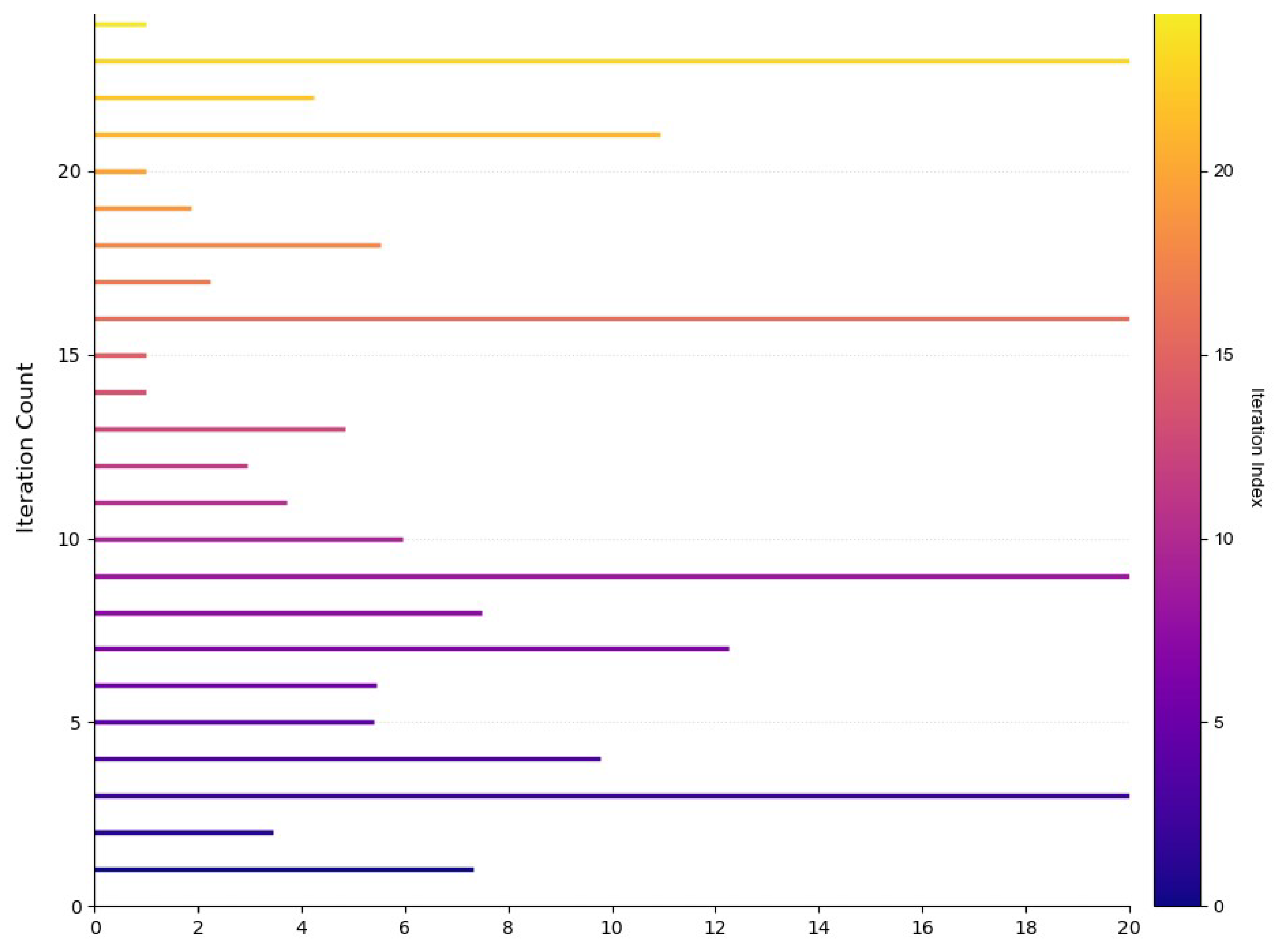
where $t\in [0,2]$; the sampling interval is 0.001; ${\left[w_k^{\left(1\right)}\left(t\right)w_k^{\left(2\right)}\left(t\right)\right]}^T$ is $\left[-0.5,0.5\right]$; the corresponding random transformation results are as shown in Figure 1; and the system’s tracking trajectory is ${\mathbf{r}}_d\left(t\right)={[2+\sin (3t),1+cos(2t\left)\right]}^T$.

1. Control Input Parameters: $a_{p,k}\left(t\right)$: The acceleration control command of the p-th vehicle at time t during the k-th iteration is measured in meters per second squared ($m/s^2$). It is a command issued by the vehicle control system to adjust vehicle speed and can be implemented by controlling actuators such as the throttle and brakes. ${\delta }_{p,k}\left(t\right)$: The steering angle control command of the p-th vehicle at time t during the k-th iteration, typically measured in radians (rad). It is used to control the vehicle’s driving direction and is executed through the steering system.

2. Nonlinear Function Parameters: $c_1$ and $c_2$: Constants used to describe nonlinear factors in the vehicle’s own motion characteristics. $c_1$ mainly reflects the resistance influence related to the first power of velocity, such as rolling friction resistance between the tires and the road surface; $c_2$ mainly reflects the resistance influence related to the square of velocity, such as air resistance. Their values need to be determined through experiments or simulations based on the vehicle’s actual performance and driving environment.

3. Control Gain Matrix Parameters: ${\alpha }_{11}$: The coefficient quantifying the influence of the acceleration control input $a_{p,k}\left(t\right)$ on the vehicle’s position $x_{p,k}\left(t\right)$. In actual vehicle motion, changes in acceleration indirectly affect the distance traveled by the vehicle over time, thereby influencing position. ${\alpha }_{11}$ quantifies this effect. ${\alpha }_{12}$: The coefficient quantifying the influence of the steering angle control input ${\delta }_{p,k}\left(t\right)$ on the vehicle’s position $x_{p,k}\left(t\right)$. Steering operations change the vehicle’s driving direction, which, in turn, affects its position. ${\alpha }_{12}$ measures this influence. ${\alpha }_{21}$: The coefficient quantifying the influence of the acceleration control input $a_{p,k}\left(t\right)$ on the vehicle’s velocity $v_{p,k}\left(t\right)$, typically related to the vehicle’s dynamic performance. It reflects the direct effect of the acceleration command on changes in vehicle velocity. ${\alpha }_{22}$: The coefficient quantifying the influence of the steering angle control input ${\delta }_{p,k}\left(t\right)$ on the vehicle’s velocity $v_{p,k}\left(t\right)$. When turning, the vehicle needs to overcome additional resistance, leading to velocity changes. ${\alpha }_{22}$ quantifies this effect. Due to the different mechanisms and degrees of influence of acceleration and steering angle on position and velocity, the $\mathbf{G}$ matrix is asymmetric, with $\mathbf{G}=[0.10.5;0.80.2]$.

Selecting the estimated matrix

$$\widehat{\mathbf{G}}=\left[\begin{array}{cc}\cos (4\pi /3)& -\sin (4\pi /3);\begin{array}{cc}-\sin (4\pi /3)& -\cos (4\pi /3)\end{array}\end{array}\right],$$

we have

$$\mathrm{spec}(-\mathbf{G}\widehat{\mathbf{G}})=\mathrm{spec}\left(-\left[\begin{array}{cc}0.1& 0.5\\ 0.8& 0.2\end{array}\right]\times \left[\begin{array}{cc}\cos (4\pi /3)& -\sin (4\pi /3)\\ -\sin (4\pi /3)& -\cos (4\pi /3)\end{array}\right]\right)$$

$$=\left\{-0.5879+0.1853i,-0.5879-0.1853i\right\}\subset C^{-}.$$

The results satisfy the conditions of the theorem. The adaptive iterative learning algorithm is evaluated using the maximum absolute error. By setting the parameter $\Gamma =5$ for the parameter update rule, Figure 2 illustrates the tracking error of the system. Figure 3 shows that the different iteration periods correspond to different lengths of tracking trajectories. It can be observed that, when the iteration count reaches 50, the tracking error of the system approaches 0. Figure 4, Figure 5, Figure 6 and Figure 7 show the trial lengths with different iterations, namely, ${\tau }_1=0.3$, ${\tau }_3=0.8$, ${\tau }_{10}=1$, and ${\tau }_{50}=2$ showing in

Table 1. Trial lengths with different iterations and tracking effects.

Iterations	Trial Length	Tracking Effect
1	${\tau }_1=0.3$	Not well tracked
3	${\tau }_3=0.8$	Not well tracked
10	${\tau }_{10}=1$	Well tracked
50	${\tau }_{50}=2$	Well tracked

, where ${\tau }_k=2$ represents the desired trial length, which demonstrates how the actual output of the system tracks the expected trajectory under varying iteration counts when subjected to non-uniform trial lengths. Figure 4 shows the actual trajectory and desired trajectory of the vehicle system at the first iteration with trial length ${\tau }_1=0.3$. Figure 5 shows the actual trajectory and desired trajectory of the vehicle system at the third iteration with trial length ${\tau }_3=0.6$. 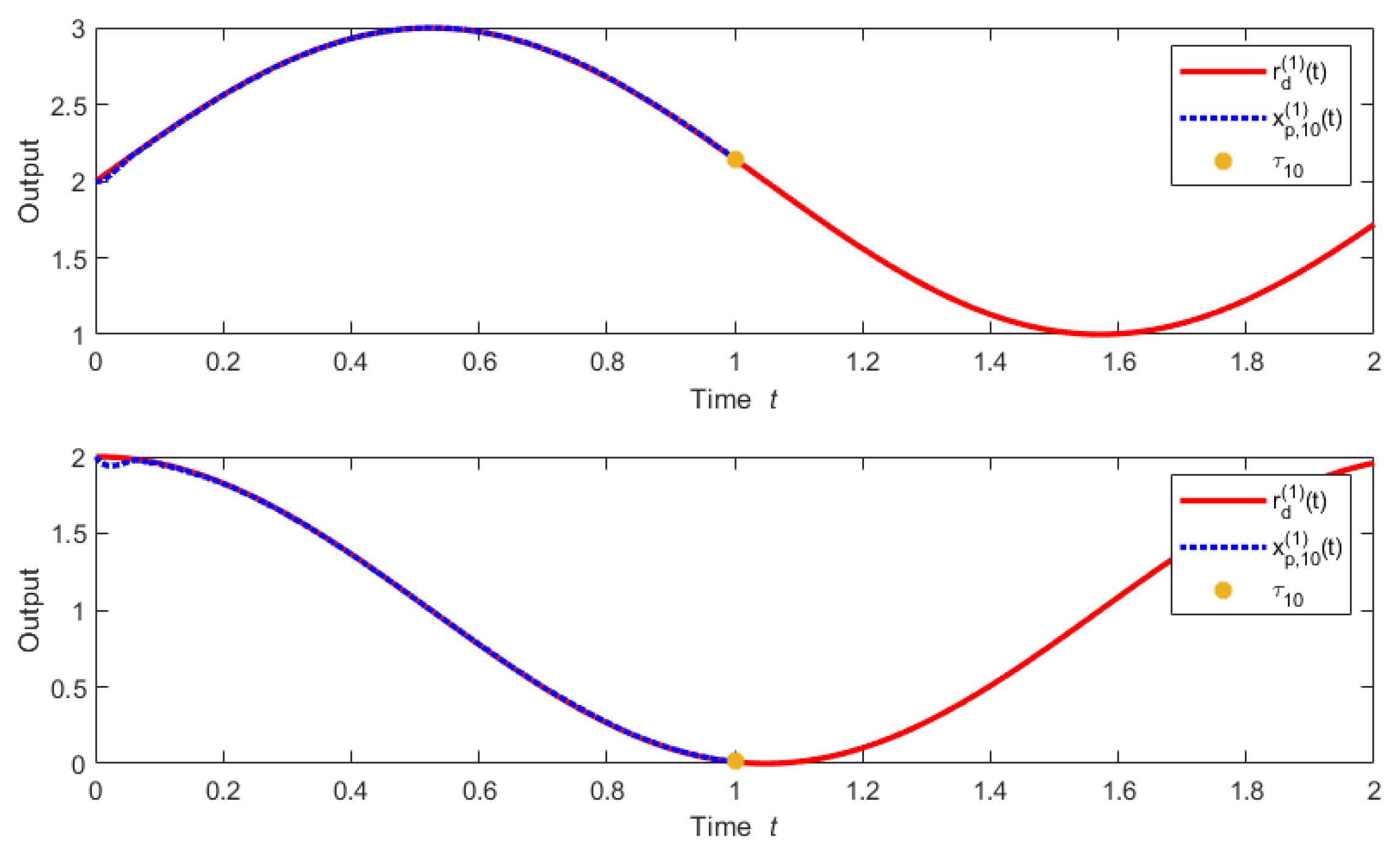Figure 6 shows the actual trajectory and desired trajectory of the vehicle system at the 10th iteration with trial length ${\tau }_{10}=1$. 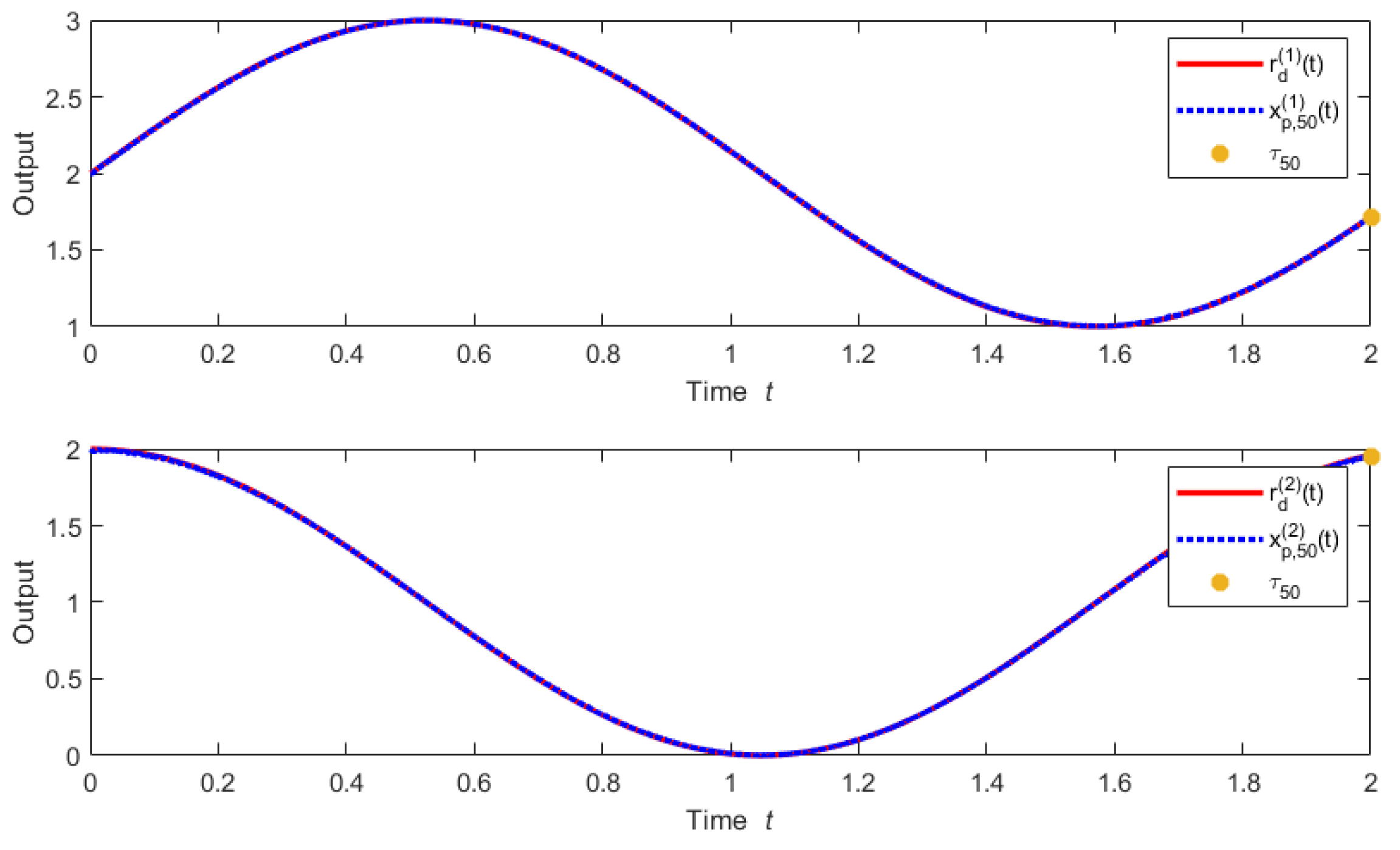Figure 7 shows the actual trajectory and desired trajectory of the vehicle system at the 50th iteration with trial length ${\tau }_{50}=2$. Notably, when the iteration number is 50, the actual output of the system fully tracks the expected trajectory. 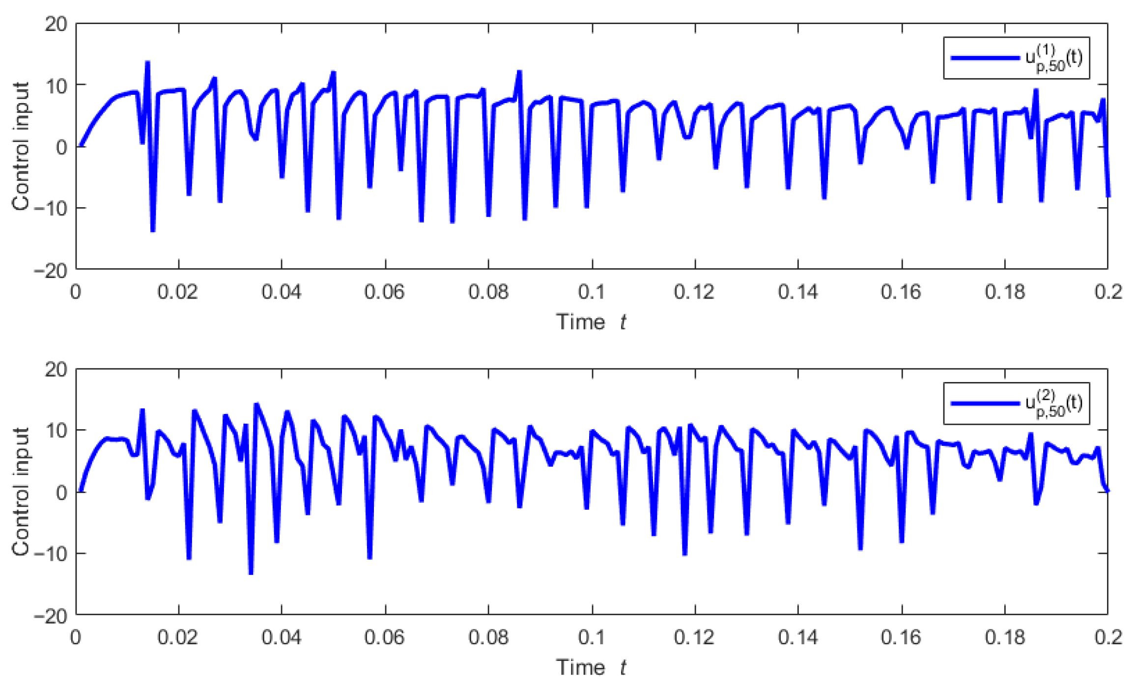Figure 8 shows the control input.

4. Conclusions

For vehicle systems with asymmetric control gain matrices, when the trial length of the system varies with the number of iterations, the system can still ensure that the tracking error tends to zero through the design of the adaptive iterative learning control algorithm. Compared with existing research on adaptive iterative learning control with non-uniform trial lengths, this paper assumes that the control gain matrix of the system is asymmetric and proves the convergence of the method by designing a Lyapunov composite energy function. The effectiveness of the method is confirmed through simulation experiments performed on a vehicle system. In future work, we will further address the additional interference (time delays or actuator failures and so on) and uncertainty modeling in nonlinear models and apply the results to actual systems.