Frequentist and Bayesian Estimation Under Progressive Type-II Random Censoring for a Two-Parameter Exponential Distribution

Abstract

In medical research, random censoring often occurs due to unforeseen subject withdrawals, whereas progressive censoring is intentionally applied to minimize time and resource requirements during experimentation. This work focuses on estimating the parameters of a two-parameter exponential distribution under a progressive Type-II random censoring scheme, which integrates both censoring strategies. The use of symmetric properties in failure and censoring time models, arising from a shared location parameter, facilitates a balanced and robust inferential framework. This symmetry ensures interpretational clarity and enhances the tractability of both frequentist and Bayesian methods. Maximum likelihood estimators (MLEs) are obtained, along with asymptotic confidence intervals. A Bayesian approach is also introduced, utilizing inverse gamma priors, and Gibbs sampling is implemented to derive Bayesian estimates. The effectiveness of the proposed methodologies was assessed through extensive Monte Carlo simulations and demonstrated using an actual dataset.

1. Introduction

Life-testing experiments are fundamental to reliability engineering, medicine, and the biological sciences for assessing the lifetime characteristics of products or individuals. However, observing the complete failure time of all units in a study is often impractical due to constraints on time, cost, or other resources. To overcome these limitations, various censoring schemes have been developed, allowing for robust statistical inference from incomplete data.

Censoring arises in two broad categories: intentional and unintentional. Intentional schemes, such as Type-I (time-based) and Type-II (failure-based) censoring, are designed by the experimenter to optimize efficiency. Among these schemes, progressive censoring has gained significant popularity for its flexibility. In a progressive censoring scheme, surviving units are strategically removed from the test at various stages, typically at the time of observed failures. This approach enhances efficiency by reducing the number of items on test over time, while providing richer data than conventional censoring. Foundational work on this topic can be found in [1,2], with numerous subsequent contributions from authors such as  [3,4,5,6,7,8].

In contrast, random censoring is an unintentional phenomenon common in clinical trials, where subjects may withdraw from a study for reasons unrelated to the primary outcome. The concept was first introduced by [9] and has been extensively studied since, with notable works by [10,11,12].

Real-world experiments often feature a combination of both planned and unplanned censoring. To model such scenarios, this study considers a progressive Type-II randomly censored (PT-IIRC) scheme. This hybrid framework, which builds on related ideas from [13,14], provides a more realistic model for many practical applications.

The lifetime model under consideration is a two-parameter exponential distribution (TExpD), characterized by a location (threshold) parameter $\mu$ and a scale parameter $\alpha$. We focus on the TExpD, due to its foundational role in reliability analysis and its mathematical properties, which allow for the clear development and illustration of the proposed inferential methods under a complex censoring scheme. The threshold parameter $\mu$ represents a guaranteed minimum lifetime. The TExpD has been widely applied in reliability analysis, with key contributions from [15,16,17,18]. A comprehensive overview is provided by [19]. While frequentist methods are well established, Bayesian approaches offer a powerful alternative for incorporating prior knowledge and handling uncertainty, especially with limited data. Seminal work in the Bayesian analysis of censored data can be found in sources like [12], who specifically addressed Bayesian analysis for exponential survival times. Our work builds on these foundations by developing a robust Bayesian framework within the more complex PT-IIRC scheme.

The primary objective of this paper was to develop and compare frequentist and Bayesian inferential methods for the parameters of the TExpD under the PT-IIRC scheme. The remainder of the article is organized as follows: Section 2 details the model formulation. Section 3 presents the MLEs and asymptotic confidence intervals. Section 4 outlines the Bayesian procedure. Section 5 provides the framework for the simulation study, and Section 6 presents a data analysis. Finally, Section 7 concludes the paper.

2. Model Formulation and Assumptions

Consider a life-testing experiment where n identical items are placed on test. The experiment is designed to terminate once a predetermined number of events, m (where $m\le n$), have been observed. Let $X_1,X_2,\dots ,X_n$ be the potential failure times of these items, assumed to be independent and identically distributed (i.i.d.) random variables. In addition to failure, each item is subject to an independent censoring time, denoted by $Y_1,Y_2,\dots ,Y_n$, which are also i.i.d. We assume that the sets $\left\{X_i\right\}$ and $\left\{Y_i\right\}$ are mutually independent.

The actual observed lifetime for item i is $Z_i=min(X_i,Y_i)$. To distinguish between failure and censoring, we define an indicator variable $d_i$ for the cause of the event

$$d_i=\left\{\begin{array}{cc}1,\hfill & \mathrm{if}{X}_i\le Y_i(\mathrm{item}\mathrm{failed}),\hfill \\ 0,\hfill & \mathrm{if}{X}_i>Y_i(\mathrm{item}\mathrm{was}\mathrm{censored}).\hfill \end{array}\right.$$

The assumption that both failure times and censoring times follow two-parameter exponential distributions with a common location parameter $\mu$, but different scale parameters ${\alpha }_1$ and ${\alpha }_2$, introduces a form of symmetry into the modeling framework. The probability density function (PDF) and survival function (SF) for the failure times (X) and censoring times (Y) are given by

$$\begin{array}{cccc}\hfill f_X(x;\mu ,{\alpha }_1)& ={\displaystyle \frac{1}{{\alpha }_1}}exp\left(-{\displaystyle \frac{x-\mu }{{\alpha }_1}}\right),\hfill & \hfill S_X(x;\mu ,{\alpha }_1)& =exp\left(-{\displaystyle \frac{x-\mu }{{\alpha }_1}}\right),x\ge \mu ,{\alpha }_1>0,\hfill \end{array}$$

(1)

$$\begin{array}{cccc}\hfill f_Y(y;\mu ,{\alpha }_2)& ={\displaystyle \frac{1}{{\alpha }_2}}exp\left(-{\displaystyle \frac{y-\mu }{{\alpha }_2}}\right),\hfill & \hfill S_Y(y;\mu ,{\alpha }_2)& =exp\left(-{\displaystyle \frac{y-\mu }{{\alpha }_2}}\right),y\ge \mu ,{\alpha }_2>0.\hfill \end{array}$$

(2)

The progressive censoring scheme is defined by a vector of integers $=(R_1,R_2,\dots ,R_m)$ such that $n=m+{\sum }_{i=1}^m{R}_i$. The experiment proceeds as follows: At the time of the first observed event, $z_{\left(1\right)}$, $R_1$ surviving items are randomly selected and removed. At the time of the second event, $z_{\left(2\right)}$, $R_2$ survivors are removed. This process continues until the m-th event at time $z_{\left(m\right)}$, at which point all remaining $R_m$ surviving items are removed and the experiment terminates.

The observed data consist of the m ordered event times, $=(z_{\left(1\right)},z_{\left(2\right)},\dots ,z_{\left(m\right)})$, and their corresponding causes, $=(d_1,d_2,\dots ,d_m)$, where $z_{\left(1\right)}<z_{\left(2\right)}<\cdots <z_{\left(m\right)}$. Here, $d_i$ is the realization of the indicator variable for the specific unit that failed or was censored at time $z_{\left(i\right)}$.

3. Maximum Likelihood Estimation

The likelihood function for progressively censored data is constructed based on the joint probability density function of the observed failure times. The contribution of each item to the likelihood depends on whether it is an observed failure, a random censoring event, or a progressively removed unit. Specifically, for an item i that fails at time $z_{\left(i\right)}$, its contribution is the joint density of failure at $z_{\left(i\right)}$ and the other process surviving past $z_{\left(i\right)}$, i.e., $f_X\left(z_{\left(i\right)}\right)S_Y\left(z_{\left(i\right)}\right)$. For an item that is randomly censored, its contribution is $f_Y\left(z_{\left(i\right)}\right)S_X\left(z_{\left(i\right)}\right)$. For each of the $R_i$ units removed at time $z_{\left(i\right)}$, their contribution is the probability of surviving past $z_{\left(i\right)}$, which is $S_X\left(z_{\left(i\right)}\right)S_Y\left(z_{\left(i\right)}\right)$. The complete likelihood is the product of these terms. For a general framework, see [2].

The likelihood function for the PT-IIRC data is given by

$$L(\mu ,{\alpha }_1,{\alpha }_2|,,)=C\prod _{i=1}^m{\left[f_X\left(z_{\left(i\right)}\right)S_Y\left(z_{\left(i\right)}\right)\right]}^{d_i}{\left[f_Y\left(z_{\left(i\right)}\right)S_X\left(z_{\left(i\right)}\right)\right]}^{1-d_i}{\left[S_X\left(z_{\left(i\right)}\right)S_Y\left(z_{\left(i\right)}\right)\right]}^{R_i}.$$

(3)

where C is a constant. Let $m_1=\sum d_i$ be the number of failures and $m_0=m-m_1$. Using Equations (1) and (2), the likelihood function in Equation (3) simplifies to

$$L(\mu ,{\alpha }_1,{\alpha }_2)\propto {\alpha }_1^{-m_1}{\alpha }_2^{-m_0}exp\left[-\left({\displaystyle \frac{1}{{\alpha }_1}}+{\displaystyle \frac{1}{{\alpha }_2}}\right)\sum _{i=1}^m(z_{\left(i\right)}-\mu )(1+R_i)\right]I(z_{\left(1\right)}\ge \mu ).$$

(4)

where $I\left(·\right)$ is the indicator function. The likelihood is maximized with respect to $\mu$ at the boundary, so the MLE is $\widehat{\mu }=z_{\left(1\right)}$. This is because the likelihood function is an increasing function of $\mu$, and its parameter space is constrained by the condition $\mu \le z_{\left(1\right)}$. Therefore, the likelihood is maximized at the boundary of the parameter space. Substituting $\widehat{\mu }$ gives the log-likelihood profile

$$\ell ({\alpha }_1,{\alpha }_2)=\mathrm{const}-m_{1}log{\alpha }_1-m_{0}log{\alpha }_2-\left({\displaystyle \frac{1}{{\alpha }_1}}+{\displaystyle \frac{1}{{\alpha }_2}}\right)T.$$

(5)

where $T={\sum }_{i=1}^m(z_{\left(i\right)}-z_{\left(1\right)})(1+R_i)$. The MLEs for the scale parameters are

$$\begin{array}{c}\hfill {\widehat{\alpha }}_1={\displaystyle \frac{T}{m_1}},\mathrm{and}{\widehat{\alpha }}_2={\displaystyle \frac{T}{m_0}}.\end{array}$$

(6)

These estimators are valid for $0<m_1<m$.

Asymptotic Confidence Intervals

To quantify the uncertainty associated with the maximum likelihood estimates, we construct confidence intervals for the unknown parameters. For the scale parameters ${\alpha }_1$ and ${\alpha }_2$, we can rely on the large-sample properties of MLEs. However, constructing a confidence interval for the location parameter $\mu$ requires a different approach, as the MLE $\widehat{\mu }=z_{\left(1\right)}$ is an order statistic and does not satisfy the standard regularity conditions for asymptotic normality. Under the standard regularity conditions detailed in texts such as [20], the distribution of the MLE vector $\widehat{\theta }={({\widehat{\alpha }}_1,{\widehat{\alpha }}_2)}^T$ can be approximated by a multivariate normal distribution. A $(1-\gamma )100\%$ asymptotic confidence interval (ACI) for ${\alpha }_1$ and ${\alpha }_2$ is given by

$$\begin{array}{cc}\hfill \mathrm{ACI}\mathrm{for}{\alpha }_1:& {\widehat{\alpha }}_1\pm {\varphi }_{1-\gamma /2}{\displaystyle \frac{{\widehat{\alpha }}_1}{\sqrt{m_1}}},\hfill \end{array}$$

(7)

$$\begin{array}{cc}\hfill \mathrm{ACI}\mathrm{for}{\alpha }_2:& {\widehat{\alpha }}_2\pm {\varphi }_{1-\gamma /2}{\displaystyle \frac{{\widehat{\alpha }}_2}{\sqrt{m_0}}}.\hfill \end{array}$$

(8)

where ${\varphi }_{1-\gamma /2}$ is the upper $(1-\gamma /2)$-th quantile of the standard normal distribution.

Constructing a confidence interval for the location parameter $\mu$ requires a different approach, as standard large-sample normality does not apply to the MLE $\widehat{\mu }=z_{\left(1\right)}$. Instead, we use an exact pivotal quantity.

Let $Z=min(X,Y)$. It follows that $Z\sim \mathrm{Exp}(\mu ,{\alpha }^{*})$, where ${\alpha }^{*}={({\alpha }_1^{-1}+{\alpha }_2^{-1})}^{-1}$. For a progressive Type-II censored sample, it is a well-known result that the following two statistics are independent [1]:

(i)

${\displaystyle \frac{2n(\widehat{\mu }-\mu )}{{\alpha }^{*}}}\sim {\chi }_{\left(2\right)}^2$

(ii)

${\displaystyle \frac{2T}{{\alpha }^{*}}}\sim {\chi }_{\left(2\right(m-1\left)\right)}^2$, where $T={\sum }_{i=1}^m(z_{\left(i\right)}-\widehat{\mu })(1+R_i)$

Here, $n=m+{\sum }_{i=1}^m{R}_i$ is the total initial sample size, and ${\chi }_{\left(k\right)}^2$ denotes a chi-squared distribution with k degrees of freedom. Taking the ratio of these two independent chi-squared variables, each divided by its degrees of freedom, forms a pivotal quantity that follows an F-distribution:

$$F={\displaystyle \frac{\left(\frac{2n(\widehat{\mu }-\mu )}{{\alpha }^{*}}\right)/2}{\left(\frac{2T}{{\alpha }^{*}}\right)/\left(2(m-1)\right)}}={\displaystyle \frac{n(m-1)(\widehat{\mu }-\mu )}{T}}\sim F_{2,2(m-1)}.$$

where $F_{2,2(m-1)}$ is an F-distribution with 2 and $2(m-1)$ degrees of freedom. A $(1-\gamma )100\%$ confidence interval for $\mu$ can be derived from the probability statement

$$P\left(F_{\gamma /2,2,2(m-1)}\le {\displaystyle \frac{n(m-1)(\widehat{\mu }-\mu )}{T}}\le F_{1-\gamma /2,2,2(m-1)}\right)=1-\gamma .$$

where $F_{q,{\nu }_1,{\nu }_2}$ is the q-th quantile of the F-distribution. Rearranging the inequality yields the exact $(1-\gamma )100\%$ confidence interval

$$\left(\widehat{\mu }-{\displaystyle \frac{T{F}_{1-\gamma /2,2,2(m-1)}}{n(m-1)}},\widehat{\mu }-{\displaystyle \frac{T{F}_{\gamma /2,2,2(m-1)}}{n(m-1)}}\right).$$

(9)

Note that this interval is valid for $m>1$.

4. Bayesian Estimation

In this section, we develop the Bayesian inference for the unknown parameters $\mu$, ${\alpha }_1$, and ${\alpha }_2$. We derive the Bayes estimates under squared error loss (SELF) and construct credible intervals using a direct Markov Chain Monte Carlo (MCMC) sampling procedure.

We assume that $\mu$, ${\alpha }_1$, and ${\alpha }_2$ are a priori independent, and for the scale parameters, we choose conjugate Inverse-Gamma priors, and for the location parameter, a non-informative uniform prior:

$$\begin{array}{cc}\hfill p\left({\alpha }_1\right)& \propto {\displaystyle \frac{1}{{\alpha }_1^{a_1+1}}}exp\left(-{\displaystyle \frac{b_1}{{\alpha }_1}}\right),{\alpha }_1>0\sim \mathrm{Inv-Gamma}(a_1,b_1),\hfill \end{array}$$

(10)

$$\begin{array}{cc}\hfill p\left({\alpha }_2\right)& \propto {\displaystyle \frac{1}{{\alpha }_2^{a_2+1}}}exp\left(-{\displaystyle \frac{b_2}{{\alpha }_2}}\right),{\alpha }_2>0\sim \mathrm{Inv-Gamma}(a_2,b_2),\hfill \end{array}$$

(11)

$$\begin{array}{cc}\hfill p\left(\mu \right)& \propto 1,-\infty <\mu <\infty .\hfill \end{array}$$

(12)

where $(a_1,b_1,a_2,b_2)$ are known hyperparameters. We choose non-informative priors to minimize the influence of prior beliefs on the posterior distribution, ensuring the inference is driven primarily by the data. This approach is standard when an objective Bayesian analysis is desired and provides a fair comparison with frequentist results.

The joint posterior distribution is obtained by multiplying the likelihood function by the priors

$$\pi (\mu ,{\alpha }_1,{\alpha }_2|data)\propto {\displaystyle \frac{1}{{\alpha }_1^{m_1+a_1+1}}}exp\left(-{\displaystyle \frac{b_1+T\left(\mu \right)}{{\alpha }_1}}\right){\displaystyle \frac{1}{{\alpha }_2^{m_0+a_2+1}}}exp\left(-{\displaystyle \frac{b_2+T\left(\mu \right)}{{\alpha }_2}}\right)I(\mu \le z_{\left(1\right)}).$$

(13)

where $m_1=\sum d_i$, $m_0=m-m_1$, and $T\left(\mu \right)={\sum }_{i=1}^m(z_{\left(i\right)}-\mu )(1+R_i)$.

To implement a direct sampling MCMC scheme, we need the marginal posterior distribution of $\mu$ and the conditional posterior distributions of ${\alpha }_1$ and ${\alpha }_2$ given $\mu$.

From the joint posterior (13), if we condition on a given value of $\mu$, the distributions for ${\alpha }_1$ and ${\alpha }_2$ are independent Inverse-Gamma distributions:

$$\begin{array}{c}\pi \left({\alpha }_1\right|\mu ,,)\sim \mathrm{Inv-Gamma}\left(m_1+a_1,b_1+T\left(\mu \right)\right),\end{array}$$

(14)

$$\begin{array}{c}\pi \left({\alpha }_2\right|\mu ,,)\sim \mathrm{Inv-Gamma}\left(m_0+a_2,b_2+T\left(\mu \right)\right).\end{array}$$

(15)

To obtain the marginal posterior distribution of $\mu$, we integrate the joint posterior with respect to ${\alpha }_1$ and ${\alpha }_2$

$$\pi \left(\mu \right|data)={\int }_0^{\infty }{\int }_0^{\infty }\pi (\mu ,{\alpha }_1,{\alpha }_2|,)d{\alpha }_{1}d{\alpha }_2.$$

This integration yields

$$\pi \left(\mu \right|data)\propto {\displaystyle \frac{\Gamma (m_1+a_1)}{{(b_1+T\left(\mu \right))}^{m_1+a_1}}}\times {\displaystyle \frac{\Gamma (m_0+a_2)}{{(b_2+T\left(\mu \right))}^{m_0+a_2}}}\times I(\mu \le z_{\left(1\right)}).$$

Since the Gamma function terms do not depend on $\mu$, we can write the kernel as

$$\pi \left(\mu \right|data)\propto {\displaystyle \frac{1}{{(b_1+T\left(\mu \right))}^{m_1+a_1}{(b_2+T\left(\mu \right))}^{m_0+a_2}}}\times I(\mu \le z_{\left(1\right)}).$$

(16)

Let $N_{prog}={\sum }_{i=1}^m(1+R_i)$ and $S_z={\sum }_{i=1}^m{z}_{\left(i\right)}(1+R_i)$. Then, $T\left(\mu \right)=S_z-\mu N_{prog}$. The cumulative distribution function (CDF) of $\mu$, needed for sampling, is

$$F\left(\mu \right)=P(\tilde{\mu }\le \mu |data)={\displaystyle \frac{{\int }_{-\infty }^{\mu }\pi \left(u\right|data)du}{{\int }_{-\infty }^{z_{\left(1\right)}}\pi \left(u\right|data)du}},\mathrm{for}\mu \le z_{\left(1\right)}.$$

(17)

This integral does not have a simple closed form and must be computed numerically. We can then sample from this distribution using the inverse CDF method.

4.1. Gibbs Sampling Algorithm

We use the following MCMC algorithm, a form of Gibbs sampling [21], to generate samples from the posterior distributions.

Step 1:

Generate from the Marginal of $\mu$

(a)

Generate a random number u from a Uniform(0,1) distribution.

(b)

Find the value ${\mu }^{*}$ that solves the equation $F\left({\mu }^{*}\right)=u$, where $F\left(·\right)$ is the CDF from Equation (17). This requires a numerical root-finding method (e.g., bisection or Newton–Raphson) as the integral is computed numerically. This ${\mu }^{*}$ is one sample from the marginal posterior of $\mu$.

Step 2:

Generate from the Conditionals of ${\alpha }_1$ and ${\alpha }_2$. Given the sampled value ${\mu }^{*}$ from Step 1,

(a)

Generate a random sample ${\alpha }_1^{*}$ from the Inverse-Gamma distribution in (14)

$${\alpha }_1^{*}\sim \mathrm{Inv-Gamma}\left(m_1+a_1,b_1+T\left({\mu }^{*}\right)\right).$$

(b)

Generate a random sample ${\alpha }_2^{*}$ from the Inverse-Gamma distribution in (15)

$${\alpha }_2^{*}\sim \mathrm{Inv-Gamma}\left(m_0+a_2,b_2+T\left({\mu }^{*}\right)\right).$$

Step 3:

Repeat for MCMC Samples Repeat Step 1 and 2 for $j=1,2,\dots ,N_{iter}$ to obtain a set of samples $\left\{({\mu }^{\left(j\right)},{\alpha }_1^{\left(j\right)},{\alpha }_2^{\left(j\right)})\right\}$.

Step 4:

Bayes Estimation. After discarding an initial burn-in period of B samples, the Bayes estimates of the parameters under SELF are obtained by averaging the remaining $N_{iter}-B$ samples

$$\begin{array}{cc}\hfill {\widehat{\alpha }}_{1,\mathrm{Bayes}}& ={\displaystyle \frac{1}{N_{iter}-B}}\sum _{j=B+1}^{N_{iter}}{\alpha }_1^{\left(j\right)},\hfill \end{array}$$

(18)

$$\begin{array}{cc}\hfill {\widehat{\alpha }}_{2,\mathrm{Bayes}}& ={\displaystyle \frac{1}{N_{iter}-B}}\sum _{j=B+1}^{N_{iter}}{\alpha }_2^{\left(j\right)},\hfill \end{array}$$

(19)

$$\begin{array}{cc}\hfill {\widehat{\mu }}_{\mathrm{Bayes}}& ={\displaystyle \frac{1}{N_{iter}-B}}\sum _{j=B+1}^{N_{iter}}{\mu }^{\left(j\right)}.\hfill \end{array}$$

(20)

4.2. Highest Posterior Density (HPD) Credible Intervals

A $100(1-\gamma )\%$ Highest Posterior Density (HPD) credible interval is the shortest possible interval containing the $(1-\gamma )$ of the posterior probability.

We estimate the HPD intervals from the MCMC samples using the algorithm proposed by [22]. For a set of N post-burn-in MCMC samples for a generic parameter $\theta$, the procedure is as follows:

• Sort the MCMC samples to obtain the ordered values: ${\theta }_{\left(1\right)}\le {\theta }_{\left(2\right)}\le \cdots \le {\theta }_{\left(N\right)}$.
• Identify all possible candidate intervals of the form $I_j=\left({\theta }_{\left(j\right)},{\theta }_{(j+k-1)}\right)$ for $j=1,\dots ,N-k+1$, where $k=\lfloor (1-\gamma )N\rfloor$.
• The HPD interval is the specific interval $I_{j^{*}}$ which has the minimum length. This is found by minimizing the difference $({\theta }_{(j+k-1)}-{\theta }_{\left(j\right)})$ over all possible values of j.

This process is applied independently to the MCMC sample sets for $\mu$, ${\alpha }_1$, and ${\alpha }_2$ to find their respective HPD credible intervals.

5. Simulation Study

To evaluate the finite-sample performance of the proposed estimation procedures, a comprehensive Monte Carlo simulation study was conducted. The true parameter values were fixed at $\mu =2.0$, ${\alpha }_1=1.5$, and ${\alpha }_2=2.0$. Various combinations of sample sizes (n) and numbers of observed failures (m) were considered under different progressive Type-II censoring schemes (R). These schemes were designed to represent diverse scenarios, including complete data (no censoring), heavy early-life censoring (e.g., $\mathbf{R}=(10,0^3)=(10,0,0,0)$), and more evenly distributed censoring patterns (e.g., $\mathbf{R}=\left({(1,0^3)}^2\right)=(1,0,0,0,1,0,0,0)$). For computing the Bayes estimates, the values of the hyperparameters were taken such that $a_1,a_2,b_1$ and $b_2$ were equal to 0.001. This choice of small, positive values is a common technique to approximate a vague or diffuse prior distribution, reflecting a lack of specific prior knowledge about the parameters. Each simulation scenario was replicated 10,000 times using the statistical software R version 4.4.2. The performance of the estimators was assessed based on four key metrics: Average Estimate (AE), Mean Squared Error (MSE), Average Interval Length (AL), and Coverage Probability (CP). For the Bayesian approach, inference was conducted via Gibbs sampling with 20,000 iterations, where the initial 2000 iterations were discarded as burn-in, to ensure convergence. The detailed results for point and interval estimation are presented in

Table 1. Performance of point estimators for different combinations of m, n, and R.

n	m	R (Scheme)	Parameter	MLE_AE	MLE_MSE	Bayes_AE	Bayes_MSE
50	50	$\left(0^{50}\right)$	$\mu$	2.0175	0.0006	2.0000	0.0003
			${\alpha }_1$	1.4906	0.0802	1.5187	0.0793
			${\alpha }_2$	2.0083	0.2056	2.0568	0.1788
50	40	$\left({(1,0^3)}^{10}\right)$	$\mu$	2.0178	0.0006	2.0001	0.0003
			${\alpha }_1$	1.5044	0.1050	1.5180	0.0417
			${\alpha }_2$	2.0298	0.2745	2.0032	0.1117
50	40	$(10,0^{39})$	$\mu$	2.0219	0.0009	2.0041	0.0005
			${\alpha }_1$	1.5059	0.1146	1.5196	0.1036
			${\alpha }_2$	2.0414	0.2849	2.0368	0.1302
50	30	$(20,0^{29})$	$\mu$	2.0287	0.0016	2.0110	0.0009
			${\alpha }_1$	1.4890	0.1458	1.5442	0.2126
			${\alpha }_2$	2.0172	0.3301	2.1859	0.2657
30	30	$\left(0^{30}\right)$	$\mu$	2.0292	0.0018	1.9998	0.0010
			${\alpha }_1$	1.4877	0.1481	1.5433	0.1150
			${\alpha }_2$	2.0242	0.4925	2.0024	0.2263
50	25	$(25,0^{24})$	$\mu$	2.0323	0.0021	2.0146	0.0013
			${\alpha }_1$	1.4717	0.1755	1.5610	0.1714
			${\alpha }_2$	2.0060	0.4541	2.0442	0.3850
50	25	$\left(1^{25}\right)$	$\mu$	2.0185	0.0007	2.0006	0.0003
			${\alpha }_1$	1.4804	0.1814	1.5698	0.1823
			${\alpha }_2$	2.0457	0.5503	2.0936	0.6920
30	25	$(5,0^{24})$	$\mu$	2.0351	0.0023	2.0052	0.0011
			${\alpha }_1$	1.4922	0.2034	1.4845	0.1216
			${\alpha }_2$	2.0673	0.5523	2.0234	0.1584
50	20	$(30,0^{19})$	$\mu$	2.0428	0.0037	2.0248	0.0025
			${\alpha }_1$	1.4918	0.2485	1.5453	0.1552
			${\alpha }_2$	2.0270	0.7585	2.0994	0.0707
30	20	$(10,0^{19})$	$\mu$	2.0433	0.0038	2.0133	0.0021
			${\alpha }_1$	1.4940	0.2458	1.7476	0.1474
			${\alpha }_2$	2.0255	0.7988	2.0030	0.1822
30	20	$\left({(1,0)}^{10}\right)$	$\mu$	2.0289	0.0017	1.9985	0.0010
			${\alpha }_1$	1.4974	0.2256	1.5490	0.1131
			${\alpha }_2$	2.0796	0.8337	2.1071	0.1511
30	15	$(15,0^{14})$	$\mu$	2.0556	0.0066	2.0246	0.0042
			${\alpha }_1$	1.5006	0.3285	1.6686	0.2739
			${\alpha }_2$	2.1015	1.3137	2.0644	0.6006

and

Table 2. Performance of confidence and credible intervals for different combinations of m, n, and R.

n	m	R (Scheme)	Parameter	ACI_AL	ACI_CP	CRI_AL	CRI_CP
50	50	$\left(0^{50}\right)$	$\mu$	0.0651	0.947	0.0651	0.946
			${\alpha }_1$	1.1086	0.926	1.1180	0.955
			${\alpha }_2$	1.7430	0.923	1.6637	0.954
50	40	$\left({(1,0^3)}^{10}\right)$	$\mu$	0.0663	0.959	0.0662	0.958
			${\alpha }_1$	1.2569	0.930	1.1165	0.951
			${\alpha }_2$	1.9826	0.934	1.3082	0.944
50	40	$(10,0^{39})$	$\mu$	0.0664	0.933	0.0665	0.933
			${\alpha }_1$	1.2583	0.922	1.2186	0.934
			${\alpha }_2$	1.9998	0.925	1.3298	0.946
50	30	$(20,0^{29})$	$\mu$	0.0669	0.897	0.0669	0.897
			${\alpha }_1$	1.4453	0.921	1.7013	0.946
			${\alpha }_2$	2.2962	0.916	2.1316	0.959
30	30	$\left(0^{30}\right)$	$\mu$	0.1111	0.938	0.1111	0.939
			${\alpha }_1$	1.4470	0.907	1.1060	0.943
			${\alpha }_2$	2.3289	0.896	2.9074	0.940
50	25	$(25,0^{24})$	$\mu$	0.0670	0.932	0.0660	0.940
			${\alpha }_1$	1.5747	0.908	1.6214	0.946
			${\alpha }_2$	2.5345	0.899	2.2969	0.953
50	25	$\left(1^{25}\right)$	$\mu$	0.0678	0.945	0.0677	0.944
			${\alpha }_1$	1.5793	0.909	1.6272	0.943
			${\alpha }_2$	2.5970	0.904	2.3886	0.944
30	25	$(5,0^{24})$	$\mu$	0.1136	0.940	0.1136	0.939
			${\alpha }_1$	1.5966	0.894	1.4506	0.943
			${\alpha }_2$	2.6385	0.905	2.4594	0.949
50	20	$(30,0^{19})$	$\mu$	0.0689	0.789	0.0689	0.785
			${\alpha }_1$	1.8089	0.912	1.3475	0.935
			${\alpha }_2$	2.9205	0.883	1.2015	0.943
30	20	$(10,0^{19})$	$\mu$	0.1149	0.902	0.1149	0.905
			${\alpha }_1$	1.8121	0.905	1.3483	0.945
			${\alpha }_2$	2.9342	0.876	2.7181	0.941
30	20	$\left({(1,0)}^{10}\right)$	$\mu$	0.1164	0.947	0.1164	0.946
			${\alpha }_1$	1.8052	0.898	1.3341	0.949
			${\alpha }_2$	3.0327	0.893	1.8529	0.944
30	15	$(15,0^{14})$	$\mu$	0.1205	0.852	0.1205	0.854
			${\alpha }_1$	2.1281	0.869	2.0567	0.941
			${\alpha }_2$	3.6647	0.891	3.2281	0.939

, respectively.

From Table 1 and Table 2, several key observations emerge:

• As expected, the estimation accuracy for all parameters improved as the number of observed failures (m) increased, leading to lower MSEs and shorter interval lengths.
• For a fixed n and m, censoring schemes with more evenly distributed removals consistently outperformed schemes with heavy early-life censoring, resulting in lower estimation errors.
• The Bayesian approach generally provided more accurate point estimates, yielding consistently lower MSEs than the MLE method, particularly for the scale parameters (${\alpha }_1,{\alpha }_2$) under censored conditions.
• The Bayesian method was substantially more reliable for interval estimation. Its Credible Intervals (CRIs) maintain coverage probabilities close to the nominal 0.95 level, whereas the MLE-based Asymptotic Confidence Intervals (ACIs) often exhibited significant undercoverage, especially in scenarios with heavy censoring.
• The location parameter $\mu$ was estimated with significantly higher precision (lower MSE) than the scale parameters ${\alpha }_1$ and ${\alpha }_2$ across all scenarios.

In summary, the simulation results suggest that the Bayesian framework is the more robust and preferable choice for inference, providing more accurate point estimates and more reliable interval estimates under the conditions studied.

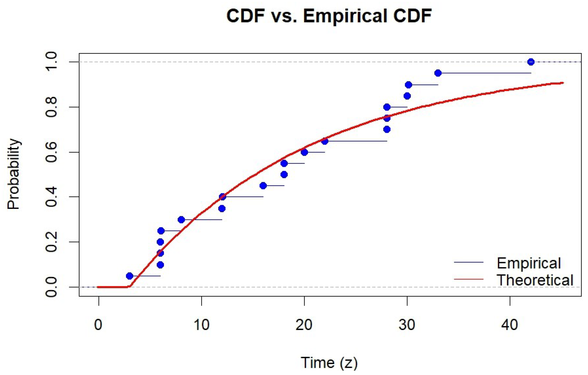
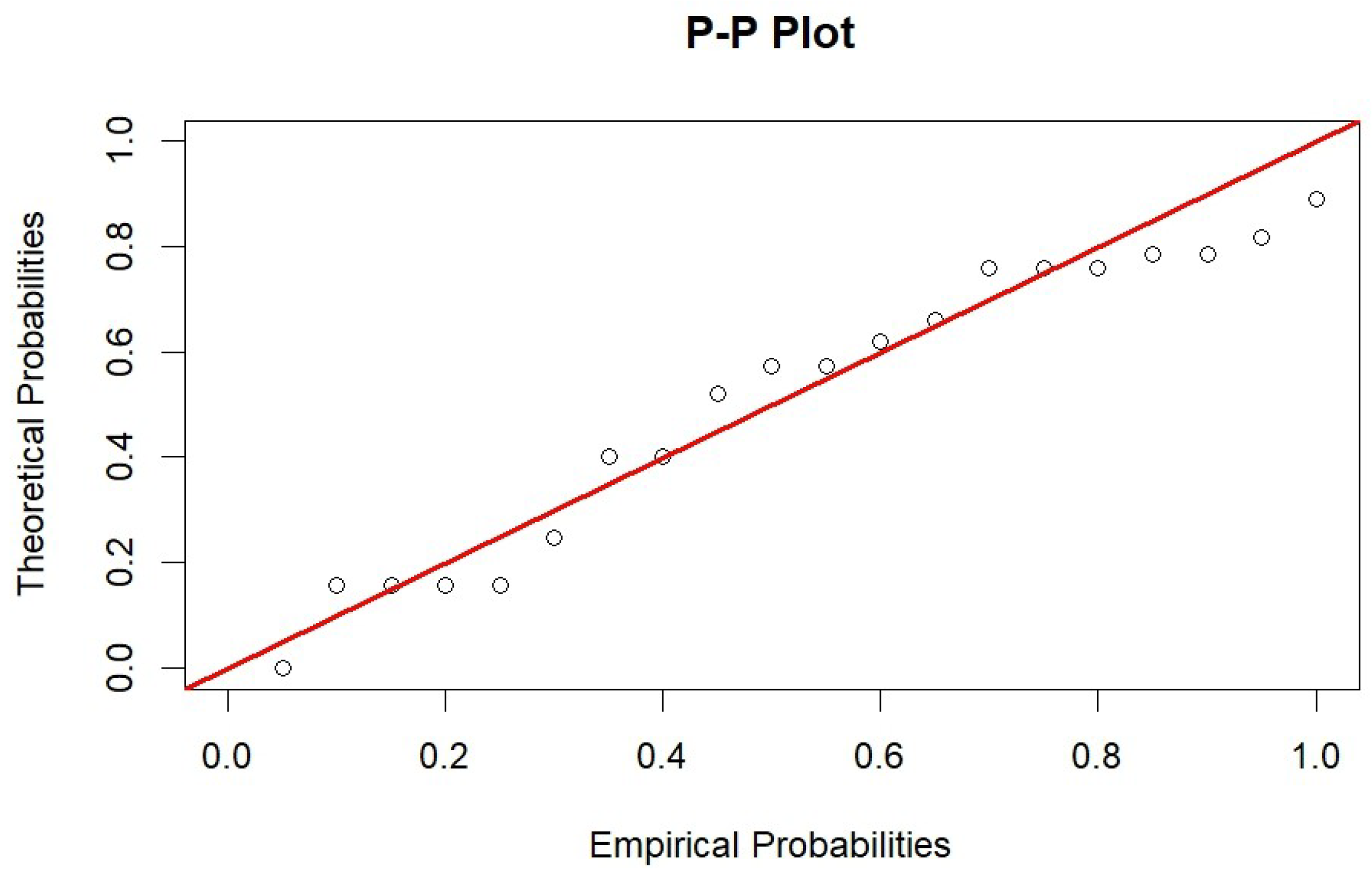
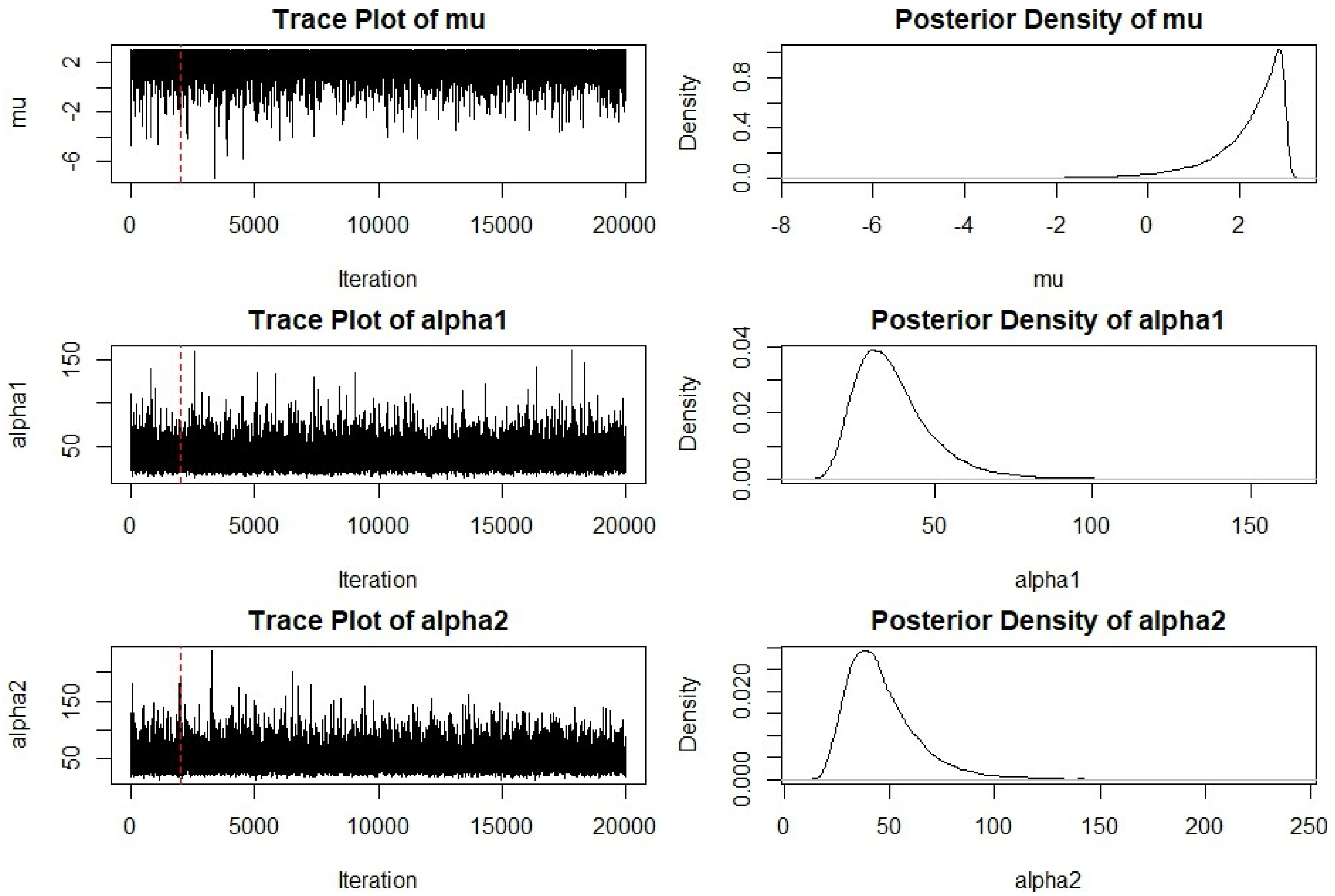
6. Real Data Analysis

To illustrate the practical application of the proposed estimation methods, we analyze a well-known dataset from the medical literature. The data, originally presented by [23], pertain to the survival times (in months) of patients with Dukes’ C colorectal cancer, and as the original study did not follow a progressive censoring protocol, we adapted the data for illustrative purposes by imposing a censoring scheme, a common practice for demonstrating new methodologies. The dataset is treated as progressive Type-II random censored and consists of the following observations:

$$\begin{array}{cc}\hfill z& =(3,6,6.01,6.02,6.03,8.01,12,12.01,16,18,18.01,20,22,28,28.01,28.02,30.01,30.1,33,42),\hfill \\ \hfill d& =(0,1,1,1,1,1,1,1,0,0,0,1,0,1,0,0,1,0,0,1),\hfill \\ \hfill R& =(0,0,0,0,1,0,0,2,0,0,0,0,1,0,0,0,0,0,0,0).\hfill \end{array}$$

Here, $d_i=1$ indicates a true failure (death), while $d_i=0$ indicates the observation was censored.

Before proceeding with parameter estimation, we assessed the goodness-of-fit of the proposed model to this dataset. The Kolmogorov–Smirnov (K-S) test, performed using R software, yielded a test statistic of D = 0.1321 and a p-value of 0.8218. Since the p-value was significantly greater than the conventional significance level of 0.05, we did not reject the null hypothesis, suggesting that the model provided an adequate fit for the data.

This conclusion is further supported by graphical diagnostics. Figure 1 shows a close alignment between the empirical and theoretical cumulative distribution functions (CDFs). Furthermore, the P-P plot (Figure 2) and Q-Q plot (Figure 3) both exhibit points lying close to the 45-degree reference line, reinforcing the conclusion that the model fit the data well.

Having established the model’s suitability, we computed both frequentist and Bayesian estimates for the parameters. For the Bayesian analysis, non-informative priors were used by setting the hyperparameters $a_1=a_2=b_1=b_2=0.0001$. The Maximum Likelihood Estimates (MLEs) with their 95% ACIs, alongside the Bayes estimates with their 95% CRI intervals, are summarized in

Table 3. Comparison of frequentist and Bayesian estimates for the real dataset.

Parameter	MLE	95% ACI	Bayes Estimate	95% CRI
$\mu$	3.0000	[0.2927, 4.9814]	2.1889	[0.0000, 2.9822]
${\alpha }_1$	32.0255	[13.1000, 50.9509]	37.0208	[19.8635, 47.7169]
${\alpha }_2$	39.1422	[13.5698, 64.7147]	46.5209	[23.1941, 71.0820]

.

To validate the Bayesian results, the convergence of the MCMC sampler was rigorously assessed, with diagnostic plots provided in Figure 4. The trace plots for all three parameters ($\mu$, ${\alpha }_1$, and ${\alpha }_2$) exhibit a stationary behavior, fluctuating rapidly around a stable central tendency with no discernible trends, which is strong evidence of successful convergence to their stationary distributions. Furthermore, we calculated the Effective Sample Size (ESS) for each parameter, and all values were well over 1000, indicating low autocorrelation in the chains and efficient estimation. The posterior density plots further reinforce this conclusion. The density for $\mu$ is appropriately bounded by the first failure time, while the densities for ${\alpha }_1$ and ${\alpha }_2$ are unimodal and well defined. This excellent MCMC performance ensures that the resulting Bayes estimates and credible intervals are reliable. While the MLE point estimates for $\mu$ and ${\alpha }_2$ appear closer to the Bayesian estimates in this specific dataset, our comprehensive simulation study (Table 1 and Table 2) provided more rigorous evidence of the Bayesian method’s overall superiority. The simulations showed that Bayesian estimators consistently yielded a lower Mean Squared Error and more reliable interval coverage across a wide range of censoring scenarios.

7. Conclusions

In this study, we successfully developed and compared frequentist and Bayesian inferential methods for the two-parameter exponential distribution under a complex progressive random censoring scheme. Our findings, from both extensive simulations and a real-data application, consistently highlight the advantages of the Bayesian approach.

The Bayesian estimators demonstrated lower mean squared errors and produced credible intervals, with coverage probabilities that were far more reliable than their frequentist counterparts, which often failed to achieve the nominal level, especially under heavy censoring. The analysis of a real-world medical dataset further validated our methodology and confirmed the stability and convergence of the proposed MCMC algorithm.

Therefore, for practitioners working with similarly complex censored data, the Bayesian framework presented here offers a more robust and accurate tool for analysis. The inherent symmetry in the model, stemming from shared structural assumptions for failure and censoring times, not only enhances inferential clarity but also contributes to computational efficiency. This symmetry-driven modeling approach provides a promising direction for further extensions.

References

1. Balakrishnan, N.; Aggarwala, R. Progressive Censoring: Theory, Methods, and Applications; Springer Science Business Media: Berlin, Germany, 2000. [Google Scholar]
2. Balakrishnan, N.; Cramer, E. The Art of Progressive Censoring; Springer: Berlin/Heidelberg, Germany, 2014; Volume 138. [Google Scholar]
3. Abu-Moussa, M.H.; Alsadat, N.; Sharawy, A. On estimation of reliability functions for the extended rayleigh distribution under progressive first-failure censoring model. Axioms 2023, 12, 680. [Google Scholar] [CrossRef]
4. Fayomi, A.; Almetwally, E.M.; Qura, M.E. Bivariate length-biased exponential distribution under progressive type-ii censoring: Incorporating random removal and applications to industrial and computer science data. Axioms 2024, 13, 664. [Google Scholar] [CrossRef]
5. Gao, X.; Gui, W. Statistical inference of burr–hatke exponential distribution with partially accelerated life test under progressively type ii censoring. Mathematics 2023, 11, 2939. [Google Scholar] [CrossRef]
6. Laumen, B.; Cramer, E. Progressive censoring with fixed censoring times. Statistics 2019, 53, 569–600. [Google Scholar] [CrossRef]
7. Lee, K. Inference for parameters of exponential distribution under combined type ii progressive hybrid censoring scheme. Mathematics 2024, 12, 820. [Google Scholar] [CrossRef]
8. Tian, Y.; Liang, Y.; Gui, W. Inference and optimal censoring scheme for a competing-risks model with type-ii progressive censoring. Math. Popul. Stud. 2024, 31, 1–39. [Google Scholar] [CrossRef]
9. Gilbert, J.P. Random Censorship. Ph.D. Thesis, University of Chicago, Department of Statistics, Chicago, IL, USA, 1962. [Google Scholar]
10. Hasaballah, M.M.; Balogun, O.S.; Bakr, M.E. On a randomly censoring scheme for generalized logistic distribution with applications. Symmetry 2024, 16, 1240. [Google Scholar] [CrossRef]
11. Krishna, H.; Goel, R. Inferences based on correlated randomly censored gumbel’s type-i bivariate exponential distribution. Ann. Data Sci. 2024, 11, 1185–1207. [Google Scholar] [CrossRef]
12. Saleem, M.; Raza, A. On bayesian analysis of the exponential survival time assuming the exponential censor time. Pak. J. Sci. 2011, 63, 44–48. [Google Scholar]
13. Goel, R.; Krishna, H. Progressive type-II random censoring scheme with Lindley failure and censoring time distributions. Int. J. Agric. Stat. Sci. 2020, 16, 23–34. [Google Scholar]
14. Goel, R.; Kumar, K.; Ng, H.K.T.; Kumar, I. Statistical inference in burr type xii lifetime model based on progressive randomly censored data. Qual. Eng. 2024, 36, 150–165. [Google Scholar] [CrossRef]
15. Beg, M. On the estimation of pr Y¡ X for the two-parameter exponential distribution. Metrika 1980, 27, 29–34. [Google Scholar] [CrossRef]
16. Cheng, C.; Chen, J.; Bai, J. Exact inferences of the two-parameter exponential distribution and pareto distribution with censored data. J. Appl. Stat. 2013, 40, 1464–1479. [Google Scholar] [CrossRef]
17. Ganguly, A.; Mitra, S.; Samanta, D.; Kundu, D. Exact inference for the two-parameter exponential distribution under type-ii hybrid censoring. J. Stat. Plan. Inference 2012, 142, 613–625. [Google Scholar] [CrossRef]
18. Krishna, H.; Goel, N. Classical and bayesian inference in two parameter exponential distribution with randomly censored data. Comput. Stat. 2018, 33, 249–275. [Google Scholar] [CrossRef]
19. Tomy, L.; Jose, M.; Veena, G. A review on recent generalizations of exponential distribution. Biom. Biostat. Int. J. 2020, 9, 152–156. [Google Scholar] [CrossRef]
20. Lehmann, E.L.; Casella, G. Theory of Point Estimation; Springer Science & Business Media: Berlin, Germany, 1998. [Google Scholar]
21. Gelf, A.E.; Smith, A.F. Sampling-based approaches to calculating marginal densities. J. Am. Stat. Assoc. 1990, 85, 398–409. [Google Scholar] [CrossRef]
22. Chen, M.; Shao, Q. Monte carlo estimation of bayesian credible and hpd intervals. J. Comput. Graph. Stat. 1999, 8, 69–92. [Google Scholar] [CrossRef]
23. McIllmurray, M.; Turkie, W. Controlled trial of gamma linolenic acid in duke’s c colorectal cancer. Br. Med. J. (Clin. Res. Ed.) 1987, 294, 1260. [Google Scholar] [CrossRef] [PubMed]
Figure 1. Empirical CDF vs. theoretical CDF for the colorectal cancer dataset.
Symmetry 17 01205 g001
Figure 2. P-P plot comparing empirical and theoretical probabilities.
Symmetry 17 01205 g002
Figure 3. Q-Q plot comparing empirical and theoretical quantiles.
Symmetry 17 01205 g003
Figure 4. MCMC convergence diagnostics: Trace plots (left) and posterior density curves (right) for parameters μ , α 1 , and α 2 .
Symmetry 17 01205 g004