Abstract
This work investigates fractional stochastic Schrödinger evolution equations in a Hilbert space, incorporating complex potential symmetry and Poisson jumps. We establish the existence of mild solutions via stochastic analysis, semigroup theory, and the Mönch fixed-point theorem. Sufficient conditions for exponential stability are derived, ensuring asymptotic decay. We further explore trajectory controllability, identifying conditions for guiding the system along prescribed paths. A numerical example is provided to validate the theoretical results.
Keywords:
exponential stability; Poisson jump; Rosenblatt process; fractional Schrödinger equation; Riemann–Liouville derivative; trajectory control MSC:
35R11; 46E20; 60G57; 47J35
1. Introduction
The Schrödinger equation (SE) is a foundational element of quantum mechanics, governing the evolution of a system’s wave function, a complex-valued function that captures the probabilistic behavior of quantum particles. While the classical SE, based on integer-order derivatives, effectively models many quantum systems, it faces limitations when dealing with phenomena exhibiting memory effects, non-locality, or anomalous diffusion. These complexities necessitate more sophisticated mathematical frameworks.
The SE plays a pivotal role in a wide range of scientific and technological domains, including atomic physics, quantum optics, semiconductor theory, and materials science. For instance, it is central to modeling light–matter interactions and predicting atomic spectra in spectroscopy. In electronics, it underpins the quantum mechanical behavior of transistors, essential components in modern computing devices (see [1,2]).
Recent advances have explored generalized formulations of the SE, particularly in contexts where stochasticity and memory effects are significant. One such generalization involves extending the SE to include fractional derivatives, giving rise to fractional Schrödinger equations (FSEs). Fractional calculus, allowing differentiation and integration of arbitrary (non-integer) order, has emerged as a powerful tool for modeling physical systems with hereditary properties [3,4,5,6,7]. The resulting FSEs enable a more accurate representation of systems governed by long-range dependencies and spatial–temporal memory [8].
Stochastic perturbations represent another key direction of generalization. Introducing randomness into the SE framework leads to stochastic Schrödinger equations (SSEs), which describe quantum systems subject to noise or uncertainty. By combining both extensions, fractional derivatives and stochasticity, one arrives at the fractional stochastic Schrödinger equation (FSSE), a powerful model for quantum systems influenced by both memory effects and random fluctuations [9,10,11,12]. These equations are especially relevant in quantum control, quantum decoherence, and the study of open quantum systems.
An important concept in the analysis of such systems is controllability, i.e., the ability to steer a system from an initial state to a target state using suitable control inputs. Trajectory controllability (TC), a more refined concept, emphasizes the capability to guide a system along a predefined path over time. This is particularly critical in quantum technologies, where precision in controlling system dynamics is essential. Chalishajar et al. [13,14] advanced the concept of TC, especially in the context of infinite-dimensional stochastic and fractional systems. Prior studies, such as [15,16,17], have explored TC for stochastic integrodifferential equations [18], motivating further exploration into FSSEs.
- Recent Developments in Fractional Schrödinger Equations:
FSEs have garnered significant attention for their capacity to model systems with non-local interactions and memory. Various analytical and numerical methods have been employed to derive exact or approximate solutions. These include the mapping method, the (G’/G)-expansion method, and spectral approaches, each yielding soliton solutions under specific conditions. Time-dependent coefficients in FSEs offer further flexibility in capturing dynamic system behavior. The Darboux transformation has also been adapted to fractional settings, enabling the generation of multi-soliton solutions and expanding the integrability of such systems. Experimental studies, including those involving Lévy waveguides and femtosecond laser pulses, have demonstrated the real-world relevance of FSEs, particularly in optical signal processing. Other studies have examined fractional Schrödinger models with singular potentials using Caputo derivatives, contributing to a deeper understanding of weak solution frameworks and their role in modeling singular quantum systems.
- Comparative Insights on Fractional Derivatives:
The choice of fractional derivative, such as the Riemann–Liouville (R–L) or Caputo derivative, plays a crucial role in modeling and interpretation. The R–L derivative, although mathematically rigorous, poses challenges such as non-zero derivatives for constants and singularities at the origin for some elementary functions. The Caputo derivative mitigates these issues, particularly allowing the incorporation of traditional initial and boundary conditions, which is critical in physical modeling [19,20,21]. Despite this, each derivative has its use cases and trade-offs, and selecting the appropriate operator depends on the specific application [22,23,24].
The problem regarding the “right” fractional derivatives is more delicate and has no unique solution. Presently, the main approach for introducing the fractional derivatives is to define them as the left-inverse operators to the fractional integrals. However, even for the R–L fractional integral, there exist infinitely many different families of operators that fulfill this property [10,25,26].
Remark 1.
- 1.
- The R–L derivative has certain disadvantages when trying to model real-world phenomena with fractional differential equations. The R–L derivative of a constant is not zero. In addition, if an arbitrary function is a constant at the origin, its fractional derivative has a singularity at the origin, for instance, the exponential and Mittag–Leffler functions. These disadvantages reduce the field of application of the R–L fractional derivative.
- 2.
- To calculate the fractional derivative of a function in the Caputo sense, we must first compute its classical derivative, which imposes stricter requirements on differentiability and regularity. It is defined only for differentiable functions. Caputo’s derivative demands higher conditions of regularity for differentiability: to compute the fractional derivative of a function in the Caputo sense, we must first calculate its derivative. Caputo derivatives are defined only for differentiable functions, while functions that have no first-order derivative might have fractional derivatives of all orders less than one in the R–L sense.
- 3.
- One of the great advantages of the Caputo fractional derivative is that it allows traditional initial and boundary conditions to be included in the formulation of the problem in a real-world situation. In addition, its derivative for a constant is zero.
- 4.
- The Caputo derivative is the most appropriate fractional operator to be used in modeling real-world problems. It is customary in groundwater investigations to choose a point on the centerline of the pumped borehole as a reference for the observations; therefore, neither the drawdown nor its derivatives will vanish at the origin, as required. In such situations where the distribution of the piezometric head in the aquifer is a decreasing function of the distance from the borehole, the problem may be circumvented using the complementary, or Weyl, fractional order derivative.
Remark 2.
To incorporate comparative experiments with existing fractional-order models, such as those based on the Caputo derivative [27], we effectively demonstrate the advantages or limitations of the R–L derivative in the proposed approach. Such a comparative analysis would provide a clearer understanding of the performance, accuracy, and potential application scope of the R–L derivative model in contrast to widely used alternatives such as the following:
- Comparative experiments enhance the credibility of the proposed method. It requires initial conditions in terms of fractional integrals, which, though more abstract, accurately reflect memory effects and non-locality, a hallmark of many physical, biological, and engineering systems. Thus, the R–L derivative is chosen when initial conditions based on fractional integrals are meaningful or required by the mathematical modeling of the system.
- It is suitable for problems where initial conditions arise naturally from fractional integrals or when the system inherently depends on past states expressed through integrals.
- It Highlights how the R–L derivative model performs relative to the Caputo model, which can strengthen the argument for choosing one over the other or reveal specific scenarios where the R–L derivative offers unique advantages, like a strong historical foundation, being non-local and memory-dependent, etc.
We summarize the same in the following chart:
| Feature | Caputo Derivative & Riemann–Liouville Derivative | |
| Definition | Derivative is applied after the integral operator. | Integral is applied after the derivative operator. |
| Initial Conditions | Accepts initial conditions in terms of integer-order derivatives (e.g., position and velocity), making it more practical for physical models. | Requires initial conditions in terms of fractional-order derivatives, which are often difficult to interpret or measure physically. |
| Physical Interpretability | More suitable for physical and engineering problems; initial conditions have clear physical meaning. | Less intuitive for real-world initial value problems due to non-local fractional initial conditions. |
| Mathematical Generality | Slightly less general than Riemann-Liouville in theory. | More general mathematically; includes a wider range of functions. |
| Zero Derivative of Constants | Caputo derivative of a constant is zero. | Riemann-Liouville derivative of a constant is non-zero. |
| Use in Initial Value Problems | Preferred in modeling real-world IVPs due to classical-style initial conditions. & Less commonly used in IVPs unless initial fractional conditions are known. | |
| Complexity in Laplace Transform | Laplace transform leads to terms with initial conditions in standard (integer-order) form. | Laplace transform results involve fractional-order initial conditions, adding complexity. |
| Computational Implementation | Easier to implement numerically for physical problems. | More challenging computationally, especially for setting bound and initial conditions. |
Remark 3.
The R-L derivative allows the construction of the fractional Schrödinger equation, which generalizes the classical Schrödinger equation. This generalization helps in the following ways:
- Modeling quantum systems where standard integer-order models fail, such as anomalous diffusion or quantum transport in fractal or porous media.
- Describing non-Markovian dynamics, which are common in realistic quantum systems.
For fractional Schrödinger systems derived from fractional path integrals or fractional Brownian motion models, the R–L derivative naturally aligns with these interpretations due to its integral-based, non-local formulation.
Remark 4.
The SE can be used to calculate the properties of a system at a given moment in time. In its time-dependent form, it describes how these properties evolve over time. SE is the fundamental equation of quantum physics, analogous to Newton’s Laws of Motion in classical physics. However, unlike Newton’s laws, the SE is not deterministic in the same way.
- In classical physics, if we know an object’s position and momentum, Newton’s Laws allow us to precisely predict its future position and momentum, provided we account for all acting forces. Newton’s laws are deterministic; they describe how forces interact and dictate the object’s trajectory at any given moment.
- In contrast, quantum mechanics introduces a different paradigm. When a photon is detected on a photographic plate, it manifests at a specific location, exposing that part of the plate to light. This does not mean that the photon initially traveled as a wave and then landed as a particle. Instead, under this interpretation, the particle does not have a defined physical reality until it is observed. The SE, in this view, serves as a mathematical tool for predicting where the particle is likely to be detected.
- Beyond this, one can analyze the TC of the particle within a fractional-order system, considering non-dynamical motion. This approach allows for a deeper exploration of quantum behavior in complex systems.
- Main Contributions of This Work:
In this study, we investigate the TC of FSSEs with complex potential symmetry using the R–L fractional derivative. The primary contributions are as follows:
- Existence of Solutions: We establish the existence of mild solutions for FSSEs using the Mönch fixed point theorem, fractional calculus, and semigroup theory.
- Stability and TC Analysis: We analyze the exponential stability of the solutions via Gronwall’s inequality and derive sufficient conditions for trajectory controllability under stochastic and memory-driven dynamics.
- Numerical Validation: Numerical simulations support the theoretical results, demonstrating how various control strategies influence system behavior in the presence of stochastic noise and fractional effects.
By integrating analytical and numerical techniques, this study deepens the understanding of control in fractional quantum systems affected by stochastic perturbations. The results have implications for both theoretical advancements and practical applications in quantum technologies.
The remainder of this paper is organized as follows: Section 2 presents definitions and preliminaries. Section 3 provides solvability results using semigroup theory and fixed-point techniques. Section 4 addresses exponential stability, while Section 5 investigates trajectory controllability. Section 6 includes a mathematical example, and Section 7 presents numerical simulations and error analysis.
2. Preliminaries
We begin this section with the abbreviation table, followed by preliminaries, which are quite useful to prove our main results.
Recently, Durga and Muthukumar [28] studied the exponential behavior of the nonlinear fractional Schrödinger evolution equation with complex potential and Poisson jumps using the strong notion called the Caputo fractional derivative (not R–L) of the following form:
| Notation | Description |
| Complete probability space with the filtration | |
| Laplace operator. | |
| Set of all real numbers. | |
| Banach space of all measurable and square-integrable values in . | |
| Separable Hilbert space with norm . | |
| Expectation of . | |
| Intervals | |
| Rosenblatt process with the Hurst parameter . |
In [29], the authors studied the fractional Schrödinger equation with potential and optimal controls of the following form:
Here, the authors used the stronger fractional derivative given by Caputo, but not R–L. Also, in both papers, the authors did not study TC and the numerical simulation of the system. The Schrödinger system with several forms is highly useful in physics and other real-life situations, and so the numerical simulation is a must.
In our study, we have used the weaker notion of Caputo called the R–L fractional order derivative with the strongest controllability called TC. Clearly, our work expands upon the work of [28] and, in a similar way, the work of [29]. More recently, Chalishajar et al. [30] investigated the optimal control problems for a class of neutral stochastic integrodifferential equations with infinite delay driven by Poisson jumps and the Rosenblatt process in Hilbert space involving concrete-fading memory-phase space, in which we define the advanced phase space for infinite delay for the stochastic process. For more details about the Rosenblatt process, one can refer to refs. [31,32].
Let us consider FSSEs with complex potential and Poisson jumps in the Hilbert space.
where , is the -order R–L derivative, and is a bound domain with a smooth boundary . Let refer to the Laplacian operator in , where is a complex-valued function in . Finally, with is a positive constant, and the function describes a potential. is the initial data.
The system (1) is transformed into a Cauchy problem by setting the state , which takes values in and is a real separable Hilbert space with the norm . We define with . Then, is the self-adjoint operator with a discrete spectrum. Next, ∃ the eigenfunctions form an orthonormal basis for with corresponding s.t , , and . is the infinitesimal generator of a strongly continuous semigroup provided by the following (according to the Hille–Yosida theorem [33]):
Let be the Poisson counting measure that is induced by the Poisson point process with the characteristic measure . Let , , and be continuous functions.
Let and be a collection of random variables known as a stochastic process. One can write instead of and Let be an -adapted Poisson point process that takes its values in , with a -finite intensity measure . An -valued random variable, denoted by , is a Banach space endowed with the norm Let be the Banach space of all continuous maps from to , satisfying the condition . Let be the closed subspace of all continuous processes that are continuous on and correspond to the space consisting of -adapted measurable processes with the norm
Fractional Brownian motion (fBm) is utilized largely due to its self-similarity, stationarity of increments, and long-range dependence (for more details see [34,35]. Tudor [36] investigated the Rosenblatt process, which is a self-similar process with stationary increments, and it appears as the limit of long-range dependent stationary series in the non-central limit theorem. Subsequently, Maejima and Tudor [37] established some new properties of the Rosenblatt distribution. It is known that the Rosenblatt process has the following properties [37]:
- (i)
- is -self-similar; that is, the processes and have identical finite-dimensional distributions .
- (ii)
- has stationary increments; that is, the finite-dimensional distribution of the process does not depend on .
- (iii)
- All the moments of the process are finite; its covariance function coincides with the covariance function of a standard fBm with the Hurst parameter :
- (iv)
- The trajectories of the Rosenblatt process are Hder continuous with an arbitrary order .
The Wiener–Ito multiple integral of order k with regard to the standard Brownian motion is as follows:
where , and the constant is a normalizing constant that ensures . Let h be a function of Hermite rank k; that is, if h admits the following expansion in Hermite polynomials
, where is the Hermite polynomial of degree j provided by . The process is called the Hermite process.
- (i)
- If , the process provided by (3) is the fBm with ;
- (ii)
- If , (3) is known as the Rosenblatt process [36].
Observation of Figure 1 says that fBm exhibits long-range dependence and self-similarity with Gaussian increments, while the Rosenblatt process (non-Gaussian and long-memory) shows more irregular and “bursty” behavior, typical of higher-order Hermite processes.
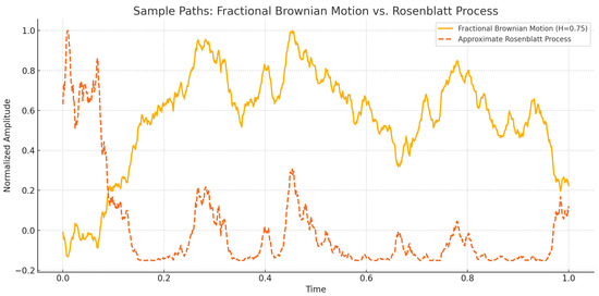
Figure 1.
The visual comparison of sample paths between fBm with Hurst parameter = 0.75, and an approximate Rosenblatt process, derived from a nonlinear transformation of fBm.
Definition 1
([37]). Let . Then,
where is a Wiener process, , is a normalizing constant, and is the kernel
here .
Definition 2
For more information and essential findings regarding the Rosenblatt process, one may consult [36,37].
Definition 3
([38,39]). The R–L fractional integral of order , for a continuous function , is defined by the following:
Definition 4
([38,40]). The R–L fractional derivative of order α of a continuous function is defined by the following:
provided is regular in its domain .
Definition 5
([38,41]). The Caputo fractional derivative of order α for a function can be defined as follows:
where denotes the derivative, provided that R.H.S is pointwise defined on .
Note: The order of is as follows:
Definition 6
([38]). The Mittag–Leffler function is defined as follows:
where denotes the complex plane. For , .
Definition 7
([38]). The Mainardi’s function is as follows:
For ,
Lemma 1
([33]). is a strongly continuous bounded operator on and .
Definition 8
([33]). A one parameter family of bounded linear operators mapping from a Banach space X into itself is said to be a strongly continuous cosine family, provided
- 1.
- is continuous in ⋉ on .
- 2.
- and
- 3.
- is a solution of (1) for all
Definition 9
([33]). The fractional sine family associated with is defined by the following:
Lemma 2
([29]). Let and . For any of ,
Lemma 3.
If then is the Lebesgue integrable.
The Housedorff MNC, , is defined as follows:
Lemma 4
([42]). Let be a Banach space and s.t,
- (1)
- is precompact; ;
- (2)
- , ;
- (3)
- , here ;
- (4)
- ;
- (5)
- ;
- (6)
- Let be a sequence of Bochner integrable functions from to with , , here , then s.t
Lemma 5
((Mönch FPT) [43]). Let be a closed convex subset of and . If is continuous and of the Mönch type, i.e., Φ is satisfied,
then, Φ has a fixed point in .
3. Main Results
Definition 10.
is a mild solution of (1) if
We make the following assumptions in order to demonstrate the existence result:
- (H1)
- (i) For , , , and operator satisfies(ii) For , ∃ s.t
- (H2)
- (i) For , and operator satisfy(ii) For , ∃ s.t
- (H3)
- (i) For a.e. , and operator satisfy(ii) A function ∃ s.t
Remark 5.
- 1.
- Physical Interpretations in Quantum Systems: In Schrödinger-type systems, the Hamiltonian or generator of the evolution may be modeled as an operator. If this operator is Lipschitz continuous, then a small change in the initial quantum state (wave function) leads to proportionally small changes in the system’s evolution. This implies robustness and predictability in how quantum states evolve over time.
- 2.
- Control Sensitivity: In quantum control theory, a control operator (e.g., coupling between system and external field) being Lipschitz continuous means that the output quantum state or observable changes is the most linear with respect to the control input. This helps to design feedback control laws and ensures that the system behaves in a predictable and tunable manner.
Existence and Uniqueness of Mild Solution
In this section, we prove the existence and uniqueness result for FSSEEs in a Hilbert space , incorporating complex symmetry and a Poisson jump.
Theorem 1.
If (H1)–(H3) hold, then (1) has a unique mild solution to
Proof.
Let be a uniform topology. It follows that and are integrable on .
To claim has a fixed point, using Lemma 1, we have , , and .
Let the operator correspond to the mild solution as follows:
The proof of the existence of the mild solution is outlined in the following four stages:
- Step 1:
- maps the bounded set in .
Let and , i.e., .
We prove that for , s.t .
Let
Thus, is bound.
- Step 2:
- is continuous in .
Let with be . For , as . Consider the following:
Hence, is continuous in .
- Step 3:
- Show that is equicontinuous.
Let . Let . If .
Now,
In a similar sense,
Using LDCT, we conclude that the RHS of the above inequalities as .
Thus, is equicontinuous.
- Step 4:
- The Mönch condition is as follows:
Set . Let us show that , where is the HMNC. Without loss of generality, we shall assume that and . Let , where
Using Hypotheses (H1) and (H2),
Thus,
So,
at least one unique mild solution for (1). □
4. Exponential Stability for FSSEs
We will now establish the exponential stability outcomes by applying the following additional requirement:
- (H4)
- For semigroups and with , there exist and , s.t
Theorem 2.
In addition, the average square of the mild solution diminishes exponentially as it approaches zero.
Proof.
Let with .
Set Consider,
Then,
Using Gronwall’s inequality,
where
Therefore, (1) decays exponentially to zero in the mean square with the exponential decay rate . □
Remark 6.
The decay condition in exponential stability has significant practical implications in real-world systems, particularly in control, quantum dynamics, and engineering applications. It guarantees that perturbations, noise, or initial excitation will vanish at an exponential rate, which is useful in quantum decoherence models (e.g., the relaxation of excited states), mechanical systems (e.g., vibrations dying out), and signal processing filters.
5. Trajectory Controllability for FSSEs
5.1. Concept of Trajectory Control
Chalishajar et al. [44] created the concept of TC, a unique and stronger notion of controllability. In TC, we want the control that directs the system along a predetermined trajectory rather than one that leads the supplied system from an initial to a desired final state. For example, while launching a rocket into orbit, knowing the exact trajectory as well as the objective destination may be helpful to maximize cost-effectiveness and prevent collisions. Nonetheless, TC results of FSSEs remain a mystery, which provides fuel for further research.
In this segment, we study TC for system (11) as follows by employing Gronwall’s inequality:
Remark 7.
Controls are always limited in some way in real-world applications. By assuming that the values of admissible controls are in a convex and closed cone with the vertex at zero, Klamka [45] investigated the sufficient conditions for constrained local relative controllability of semilinear ordinary differential state equations in finite dimensions with delayed controls using a generalized open-mapping theorem. The restricted complete controllability of first- and second-order systems in infinite-dimensional space was also demonstrated by Klamka [45]. Our system can be extended for fractional-order systems, and the TC result can be examined.
Remark 8.
TC in quantum mechanics refers to the ability to steer a quantum system’s state along a desired trajectory over time using external controls (e.g., electromagnetic fields and laser pulses). While the term is rooted in control theory, it finds growing use in quantum control, a field at the intersection of quantum physics and systems engineering. Quantum optimal control is finding optimal pulse sequences to transfer populations between quantum states or to create entanglement. Example: Controlling spin systems, two-level atoms, or molecules with laser fields.
5.2. Definition, Lemma, and Main Theorem
Here, we provide the TC definition of the system (11), as we know that the control definition varies from system to system.
Definition 11.
Lemma 6
([46]). Let and be a locally integrable function on and be a non-negative, non-decreasing continuous function on , , where is a constant. Also, , then
In particular, when , then .
Let us now consider system (1) with the control term , as shown below:
The mild solution of (11) is as follows:
Theorem 3.
(H1)–(H4) assure the TC of (12) on
Proof.
Let be a trajectory on . Let us choose the feedback control as follows:
Thus, (11) implies the following:
Setting ,
Thus,
where .
Using Lemma 6,
Hence, (11) is TC on . □
Remark 9.
Computational Tractability of Implementing Controls in Real Systems: In real systems, the computational tractability of implementing control strategies hinges on the balance between model complexity and real-time performance requirements. While advanced control laws (e.g., model predictive control, fractional-order, or sliding mode control) offer high precision and robustness, they often involve nonlinear equations, memory effects, or optimization problems that are computationally intensive. In practice, nonlinear and fractional-order controls, though theoretically powerful, may become intractable in high-dimensional or fast-evolving systems without significant simplification or approximation. Hardware constraints, communication delays, and the need for fast sampling rates further limit the feasibility of complex control laws in many industrial or robotic applications. Thus, achieving computational feasibility often requires model reduction, efficient numerical algorithms, or approximate control schemes that preserve key dynamics while remaining implementable on available platforms.
6. Comprehensive Analysis Between Exact and Numerical Solutions
6.1. Theoretical Example for FSSEs
The theoretical example of our study is demonstrated as follows.
Consider,
where , is the -order R–L fractional operator. Let and . Let . Let generate eigenvalues with associated eigenfunctions . The set is an orthonormal basis of .
Define and the nonlinear functions as follows:
and
The above nonlinear functions satisfy the conditions (H1)–(H4). Thus, all the hypotheses of Theorem 1 are satisfied. So, the system (1) has a mild solution. We choose the particular values of the given parameters as follows: with .
Further, the following numerical values fulfill the condition of Theorem 2:
The mild solution (1) decays exponentially to zero in the mean square.
6.2. Numerical Simulation for FSSEs
This subsection studies the simulation of the system (13) numerically with detailed justification. By adopting this integrated approach, we create a cohesive narrative that effectively bridges theory and practice, enhancing the clarity and impact of our research.
The numerical simulation of the fractional stochastic Schrödinger equation involves using various techniques to approximate the solutions to this complex equation, which describes quantum systems influenced by both fractional derivatives and random noise. These simulations are crucial for understanding the behavior of quantum systems in non-standard environments, such as those with fractal or noisy potentials.
Researchers have numerically simulated the system’s accuracy in a number of methods (refer to [13] for more details). The normalized Bernstein wavelets method will be applied in this part. Fractional partial differential Equation (13) is solved using the fractional order integration and Bernstein wavelets operating matrices of integration. The efficiency of the suggested approach is demonstrated using the root mean square error and maximum absolute error in the event of having the exact solution. The boundary conditions are automatically taken into account in the proposed method. Additionally, a normalized Bernstein wavelet-based evaluation of the error of function approximation is employed. The Legendre wavelet approach and the Bernstein wavelet method are contrasted. Every calculation related to the examples is carried out using Mathematica 9.1 running on a Windows 10 PC with 4 GHz processing speed and 4 GB of DDR3 memory. For convenience, we assume that = X.
The following table shows the root mean square error and maximum absolute error in some nodes . To show the efficiency of this method, the absolute error obtained by the present method is compared with the Legendre wavelet method [47] in the Table below. Figure 1 and Figure 2 represent the error analysis for = 0.50, 0.90, and 1.00, respectively. We compare the numerical solution with the exact solution for = 0.50, 0.90, and 1.00 in Figure 3, Figure 4 and Figure 5, respectively. It is evident from last two rows of Table below and Figure 3, Figure 4 and Figure 5 that the proposed method is accurate for solving this kind of problem, and the obtained approximate solution is very close to the exact one.
| (in Seconds) | ||||||
| Legendre wavelet method [47] | ||||||
| Bernstein wavelet method |
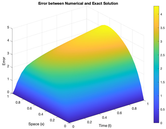
Figure 2.
Error analysis of an exact and numerical solution: = 0.50. Here, = X and t = ⋉ in seconds: real traveling wave solutions.
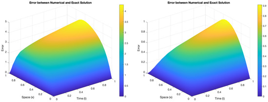
Figure 3.
Error analysis = 0.50 (left) and error analysis = 0.90 (right). Here, = X and t = ⋉ in seconds.
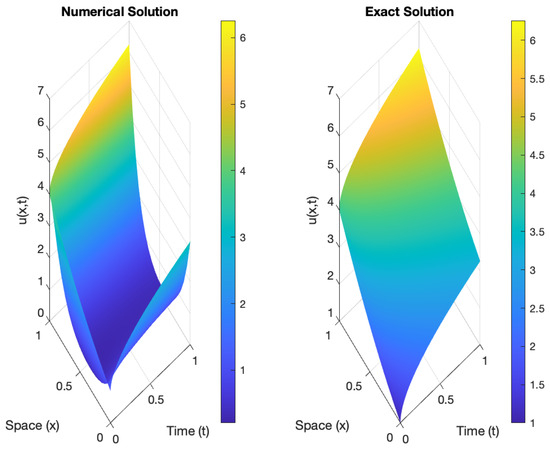
Figure 4.
Comparison of a control for the exact and numerical solutions for the order = 0.50 in a state.
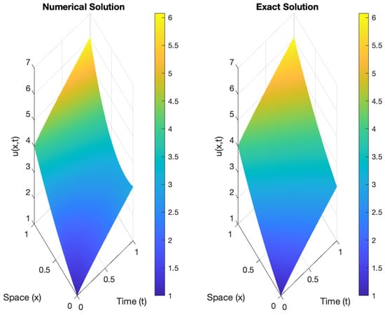
Figure 5.
Comparison of a control for the exact and numerical solutions for the order = 0.90 in a state.
Three-dimensional real and imaginary traveling wave solutions for Equation (13) are depicted as follows: real traveling wave solutions in Figure 1 and imaginary traveling wave solutions in Figure 2. The mild solution diminishes exponentially as it approaches zero (kindly refer to Table 1). The control goes along the prescribed trajectory with absolutely small errors for different fractional values of , as described within the interval [0, 1]. This analysis of numerical simulation justifies the theory provided in Figure 3, Figure 4 and Figure 5. The comparison of Figure 3, Figure 4 and Figure 5 clearly shows that as the value of approaches 1, the error reduces and the approximations move closer together.
Figure 1 and Figure 2 illustrate the differences in the 3D particle distribution between the FSE with the Dirac delta function and the classical one. This indicates that peaks appear in the distribution; namely, a gap appears at in Figure 1 and Figure 2. The reason is that diffusion only occurs along the x-axis. In addition, we see that the particle distribution in Figure 3, Figure 4 and Figure 5 is symmetric about the x-axis and y-axis because the velocity only has an effect on the distribution at for quantum diffusion. Figure 3(left) is similar to a waveform, Figure 3(right), because of the influence of the singularity function in 3D. Figure 4 fully demonstrates the influence of the singularity function on the FSE with changing time. The larger time parameter ⋉ leads to faster particle diffusion. A smaller parameter produces a stronger wave characteristic. Furthermore, a larger fractional parameter results in faster particle diffusion. The mass parameter is a proportional constant between the momentum and energy, which is used to describe the mass of the quantum. A larger mass produces a weaker wave characteristic. Larger mass indicates faster diffusion.
The trapezoid rule, as implemented by the MATLAB function trapz.m, was used to approximate the integral term at each discretization point. The Brownian term is normally distributed with mean zero and variance . The fractional Brownian term is normally distributed with mean zero and variance , where h is the Rossenblatt parameter. The delayed derivative terms were approximated by difference derivatives on the mesh as well. One of the more challenging parts of approximating numerical solutions to this equation is the delay terms inside both the time and space derivatives. In order to apply the finite difference formulas, the derivative operator must be applied to these terms and formulas derived.
In the included simulations (Figure 4, Figure 5 and Figure 6), the following parameters were used. We used and 20 points in each spatial dimension for a total of 400 spatial points at each timestep. We used 5000 timesteps, so . The Rossenblatt parameter . Figure 2 and Figure 3 show the function at the beginning, at , and a third of the way through the simulation. Figure 4, Figure 5 and Figure 6 show the simulation at roughly two-thirds of the way through the simulation and at the end. The Poisson jump intensity (sometimes called the rate or arrival rate) with respect to time ⋉ is quite significant, occurring at specific points in time in Figure 4, Figure 5 and Figure 6. It defines the expected number of jumps per unit of time. Also, Figure 3, Figure 4, Figure 5 and Figure 6 suggest that the dispersion rate of the wavefunction is inversely proportional to mass: heavier particles spread more slowly and lighter particles (like electrons) exhibit more pronounced quantum spreading. This affects how quickly the probability distribution for position becomes wider over time.
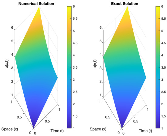
Figure 6.
Comparison of a control for the exact and numerical solutions for the order = 1.00 in a state.
Since this is an optimization problem over two spatial dimensions and one time dimension, it can quickly become computationally infeasible. We used five points in each spatial dimension and 10 points in the time dimension, which still left us with 250 total control points to optimize for. In the first stage of optimization, we used the Legendre wavelet algorithm, as implemented in the MATLAB function. Figure 4 contains the error of the function before the first stage of optimization began at two time points. Note that the order of error is approximately 1. Figure 5 contains the error after 200,000 iterations of the Bernstein wavelet algorithm were applied. Note that the order magnitude is approximately , a significant improvement over Figure 4. Figure 6 shows the error after 5000 iterations of the Bernstein wavelet algorithm. Note that the order of magnitude is approximately , which is much better than Figure 4. Thus, illustrating the example equation can be made to follow a given trajectory, using optimization to determine the appropriate control.
Remark 10.
To estimate computational cost, we break the problem down into the following components:

Table 1.
Steps to estimate the computational cost of a Schrödinger stochastic control system.
Table 1.
Steps to estimate the computational cost of a Schrödinger stochastic control system.
| Step | What to Do |
|---|---|
| 1 | Define the model’s resolution, i.e., the number of spatial points , time steps , and stochastic samples . |
| 2 | Identify the numerical method used (e.g., finite differences, Bernstein wavelets, and spectral methods). |
| 3 | Include the effect of control logic, especially if it involves feedback, delay, or adaptive terms. |
| 4 | Benchmark and validate performance on your actual hardware using profiling tools or runtime measurement. |
7. Conclusions
The above investigation focused on the existence, uniqueness, time complexity, and exponential stability of FSSEs that incorporate complex potentials and Poisson jumps. The primary findings are founded on the principles of stochastic analysis, fractional calculus, and Mönch FPT. Additionally, the results demonstrate mean square exponential stability along with the corresponding time complexity. In this work, we used the weaker notion of the fractional derivative called the R–L derivative. The current study explored FSSEs using R–L fractional derivatives, which offer certain mathematical conveniences but are also known to impose restrictions due to their non-local initial condition requirements. The R–L fractional derivative plays a meaningful role in modeling the non-locality of quantum mechanics, especially in generalized quantum theories and open quantum systems where classical Schrödinger dynamics are extended to include memory, dissipation, or anomalous transport. Non-locality refers to correlations or entanglement between spatially separated particles. R–L derivatives help describe non-local environments or long-range interactions between a system and its reservoir.
An interesting extension of this work would be to consider generalized fractional derivatives, particularly the Hilfer derivative, which interpolates between the R–L and Caputo derivatives. The Hilfer framework allows for greater modeling flexibility and can bridge the gap between different fractional orders and initial condition formulations. This direction may open up avenues for the following: Comparative analysis of solution behavior under different fractional operators; Broader classes of initial-boundary value problems; More physically meaningful interpretations in memory-driven or anomalously diffusive quantum systems.
Incorporating Hilfer-type derivatives could enhance the robustness of the controllability and stability results and potentially unify various fractional approaches under a more generalized theory. The system introduced can be extended further to include a fractional Schrödinger equation that integrates mixed fBm with both instantaneous and non-instantaneous impulses. The Clarke subdifferential approach may facilitate further exploration of the topic. The role of noise in quantum systems is still debated, especially in the context of open quantum systems. The numerical treatment of fractional derivatives and stochastic terms can be computationally expensive. Standard numerical methods may not work efficiently, requiring fractional-order adaptations. The memory effects induced by fractional derivatives may require non-traditional boundary conditions.
Author Contributions
Conceptualization: D.C., R.K. (Ravikumar Kasinathan), R.K. (Ramkumar Kasinathan) and D.K.; Methodology: R.K. (Ravikumar Kasinathan), R.K. (Ramkumar Kasinathan) and D.K.; Software: R.K. (Ravikumar Kasinathan) and D.K.; Formal analysis: D.C.; Investigation: D.C.; Data curation: R.K. (Ravikumar Kasinathan) and R.K. (Ramkumar Kasinathan); Writing—original draft: R.K. (Ramkumar Kasinathan); Writing—review & editing, H.T.; Project administration: D.C. All authors have read and agreed to the published version of the manuscript.
Funding
No funding is available to the conduct this research.
Data Availability Statement
The original contributions presented in this study are included in the article. Further inquiries can be directed to the corresponding authors.
Conflicts of Interest
Authors declear that they do not have any conflicts of interest.
References
- Chen, J. Strichartz type estimates for solutions to the Schrödinger equation. Proc. Amer. Math. Soc. 2024, 152, 3941–3953. [Google Scholar] [CrossRef]
- Karjanto, N. Modeling Wave Packet Dynamics and Exploring Applications: A Comprehensive Guide to the Nonlinear Schrödinger Equation. Mathematics 2024, 12, 744. [Google Scholar] [CrossRef]
- Keten, A.; Yavuz, M.; Baleanu, D. Nonlocal Cauchy Problem via a Fractional Operator Involving Power Kernel in Banach Spaces. Fractal Fract. 2019, 3, 27. [Google Scholar] [CrossRef]
- Manigandan, M.; Muthaiah, S.; Nandhagopal, T.; Vadivel, R.; Unyong, B.; Gunasekaran, N. Existence results for coupled system of nonlinear differential equations and inclusions involving sequential derivatives of fractional order. Aims Math. 2022, 7, 723–755. [Google Scholar] [CrossRef]
- Seralan, V.; Vadivel, R.; Gunasekaran, N. Fractional-Order Dynamics and Fear-Induced Bifurcation in Delayed Food Chain Model. Int. J. Bifurc. Chaos Appl. Sci. 2025, 35, 2550079. [Google Scholar] [CrossRef]
- Triggiani, R. A note on the lack of exact controllability for mild solutions in Banach spaces. SIAM J. Control Optim. 1977, 15, 407–411. [Google Scholar] [CrossRef]
- Yavuz, M. European option pricing models described by fractional operators with classical and generalized Mittag-Leffler kernels. Numer. Methods Partial. Differ. Equ. 2022, 38, 434–456. [Google Scholar]
- Abbas, M.I. Existence results and the Ulam stability for fractional differential equations with hybrid proportional-Caputo derivatives. J. Nonlinear Funct. Anal. 2020, 2020, 48. [Google Scholar] [CrossRef]
- Ahmed, H.M. Semilinear neutral fractional stochastic integro-differential equations with nonlocal conditions. J. Theor. Probab. 2015, 28, 667–680. [Google Scholar] [CrossRef]
- Kaslik, E.; Sivasundaram, S. Nonlinear dynamics and chaos in fractional-order neural networks. Neural Netw. 2012, 32, 245–256. [Google Scholar] [CrossRef] [PubMed]
- Kumar, S.; Kumar, D.; Singh, J. Numerical computation of fractional Black–Scholes equation arising in financial market. Egyptian J. Basic. Appl. Sci. 2014, 1, 177–183. [Google Scholar] [CrossRef]
- Kumar, D.; Seadawy, A.R.; Joardar, A.K. Modified Kudryashov method via new exact solutions for some conformable fractional differential equations arising in mathematical biology. Chin. J. Phys. 2018, 56, 75–85. [Google Scholar] [CrossRef]
- Chalishajar, D.; Chalishajar, H. Trajectory Controllability of Second Order Nonlinear Integro-Differential System: An Analytical and a Numerical Estimation. Differ. Equ. Dyn. Syst. 2015, 23, 467–481. [Google Scholar] [CrossRef]
- Chalishajar, D.N.; George, R.K.; Nandakumaran, A.K.; Acharya, F.S. Trajectory controllability of nonlinear integro-differential system. J. Frank. Inst. 2010, 347, 1065–1075. [Google Scholar] [CrossRef]
- Dhayal, R.; Malik, M.; Abbas, S. Approximate and trajectory controllability of fractional stochastic differential equation with non-instantaneous impulses and Poisson jumps. Asian J. Control 2021, 23, 2669–2680. [Google Scholar] [CrossRef]
- Ramkumar, K.; Ravikumar, K.; Chalishajar, D. Existence trajectory and optimal control of Clarke subdifferential stochastic integrodifferential inclusions suffered by non-instantaneous impulses and deviated arguments. Results Control Optim. 2023, 13, 100295. [Google Scholar] [CrossRef]
- Baleanu, D.; Kasinathan, R.; Kasinathan, R.; Srasekaran, V. Existence, uniqueness and Hyers-Ulam stability of random impulsive stochastic integro-differential equations with nonlocal conditions. AIMS Math. 2023, 8, 2556–2575. [Google Scholar] [CrossRef]
- Muslim, M.; Kumar, A.; Sakthivel, R. Exact and trajectory controllability of second-order evolution systems with impulses and deviated arguments. Math. Methods Appl. Sci. 2018, 41, 4259–4272. [Google Scholar] [CrossRef]
- Alzaidy, J.F. Fractional sub-equation method and its applications to the space-time fractional differential equations in mathematical physics. Br. J. Math. Comput. Sci. 2013, 3, 153–163. [Google Scholar] [CrossRef] [PubMed]
- Baleanu, D.; Diethelm, K.; Scalas, E.; Trujillo, J.J. Fractional Calculus Models and Numerical Methods; World Scientific: Singapore, 2012. [Google Scholar]
- Ding, Y.; Wang, Z.; Ye, H. Optimal control of a fractional-order HIV-immune system with memory. IEEE Trans. Control. Syst. Technol. 2011, 20, 763–769. [Google Scholar] [CrossRef]
- Koh, C.G.; Kelly, J.M. Application of fractional derivatives to seismic analysis of base isolated models. Earthq. Eng. Struct. Dyn. 1990, 19, 229–241. [Google Scholar] [CrossRef]
- Miller, K.S.; Ross, B. An Introduction to the Fractional Calculus and Fractional Differential Equations; Wiley-Interscience, John-Wiley and Sons: New York, NY, USA, 1993. [Google Scholar]
- Podlubny, I. Fractional Differential Equations; Academic Press: San Diego, CA, USA, 1999. [Google Scholar]
- Islam, M.N.; Koyuncuoğlu, H.C.; Raffoul, Y.N. A Note on the Existence of Solutions for Caputo Fractional Differential Equations. J. Integral Equ. Appl. 2024, 36, 437–446. [Google Scholar] [CrossRef]
- Jin, T.; Yang, X. Monotonicity theorem for the uncertain fractional differential equation and application to uncertain financial market. Math. Comput. Simul. 2021, 190, 203–221. [Google Scholar] [CrossRef]
- Gunasekaran, N.; Manigandan, M.; Vinoth, S.; Vadivel, R. Analysis of Caputo Sequential Fractional Differential Equations with Generalized Riemann–Liouville Boundary Conditions. Fractal Fract. 2024, 8, 457. [Google Scholar] [CrossRef]
- Durga, N.; Muthukumar, P. Exponential Behaviour of Nonlinear Fractional Schrödinger Evolution Equation with Complex Potential and Poisson Jumps. J. Theor. Probab. 2023, 36, 1939–1955. [Google Scholar] [CrossRef]
- Wang, J.; Zhou, Y.; Wei, W. Fractional Schrödinger equations with potential and optimal controls. Nonlinear Anal. 2012, 13, 2755–2766. [Google Scholar] [CrossRef]
- Chalishajar, D.; Kasinathan, R.; Kasinathan, R. Optimal control for neutral stochastic integrodifferential equations with infinite delay driven by Poisson jumps and rosenblatt process. Fractal Fract. 2023, 7, 783. [Google Scholar] [CrossRef]
- Lakhel, E.H.; McKibben, M.A. Controllability for time-dependent neutral stochastic functional differential equations with Rosenblatt process and impulses. Int. J. Control Autom. Syst. 2019, 17, 112. [Google Scholar] [CrossRef]
- Dhanalakshmi, K.; Balasubramaniam, P. Stability result of higher-order fractional neutral stochastic differential system with infinite delay driven by Poisson jumps and Rosenblatt process. Stoch. Anal. Appl. 2020, 38, 352–372. [Google Scholar] [CrossRef]
- Pazy, A. Semigroups of Linear Operators and Applications to Partial Differential Equations; Springer: New York, NY, USA, 1983. [Google Scholar]
- Mishura, Y.S. Stochastic Calculus for Fractional Brownian Motion and Related Processes; Springer: Berlin/Heidelberg, Germany, 2008. [Google Scholar]
- Koyuncuoğlu, H.C.; Raffoul, Y.; Turhan, N. Asymptotic constancy for the solutions of Caputo fractional differential equations with delay. Symmetry 2022, 15, 88. [Google Scholar] [CrossRef]
- Tudor, C.A. Analysis of the Rosenblatt process. ESAIM Prob. Stat. 2008, 12, 230257. [Google Scholar] [CrossRef]
- Maejima, M.; Tudor, C.A. On the distribution of the Rosenblatt process. Stat. Prob. Lett. 2013, 83, 14901495. [Google Scholar] [CrossRef]
- Kilbas, A.A.; Srivastava, H.M.; Trujillo, J.J. Theory and Applications of Fractional Differential Equations; Elsevier B. V.: Amsterdam, The Netherlands, 2006. [Google Scholar]
- Ramkumar, K.; Ravikumar, K.; Varshini, S. Fractional neutral stochastic differential equations with Caputo fractional derivative: Fractional Brownian motion, Poisson jumps, and optimal control. Stoch. Anal. Appl. 2021, 39, 157–176. [Google Scholar] [CrossRef]
- Anguraj, A.; Ramkumar, K. Approximate controllability of semilinear stochastic integrodifferential system with nonlocal conditions. Fractal Fract. 2018, 2, 29. [Google Scholar] [CrossRef]
- Caputo, M.; Fabrizio, M. A new definition of fractional derivative without singular kernel. Prog. Fract. Differ. Appl. 2015, 1, 73–85. [Google Scholar]
- Burton, T.A. A fixed-point theorem of Krasnoselskii. Appl. Math. Lett. 1998, 11, 8588. [Google Scholar] [CrossRef]
- Mao, X. Stochastic Differential Equations and Applications; Horwood: Chichester, UK, 1997. [Google Scholar]
- Chalishajar, D.N.; George, R.K.; Nandakumaran, A.K. Exact controllability of the nonlinear third-order dispersion equation. J. Math. Anal. Appl. 2007, 332, 1028–1044. [Google Scholar] [CrossRef]
- Klamka, J. Constrained controllability of semilinear systems with delays. Nonlinear Dyn. 2009, 56, 169–177. [Google Scholar] [CrossRef]
- Chalishajar, D.; Kasinathan, R.; Kasinathan, R.; Kasinathan, D.; David, J.A. Trajectory controllability of neutral stochastic integrodifferential equations with mixed fractional Brownian motion. J. Control Decis. 2023, 12, 351–365. [Google Scholar] [CrossRef]
- Heydari, M.H.; Hooshmandasl, M.R.; Mohammadi, F. Legendre wavelets method for solving fractional partial differential equations with Dirichlet boundary conditions. Appl. Math. Comput. 2024, 234, 267–276. [Google Scholar] [CrossRef]
Disclaimer/Publisher’s Note: The statements, opinions and data contained in all publications are solely those of the individual author(s) and contributor(s) and not of MDPI and/or the editor(s). MDPI and/or the editor(s) disclaim responsibility for any injury to people or property resulting from any ideas, methods, instructions or products referred to in the content. |
© 2025 by the authors. Licensee MDPI, Basel, Switzerland. This article is an open access article distributed under the terms and conditions of the Creative Commons Attribution (CC BY) license (https://creativecommons.org/licenses/by/4.0/).