
Exploring Solitary Wave Solutions of the Generalized Integrable Kadomtsev–Petviashvili Equation via Lie Symmetry and Hirota’s Bilinear Method


Abstract
1. Introduction
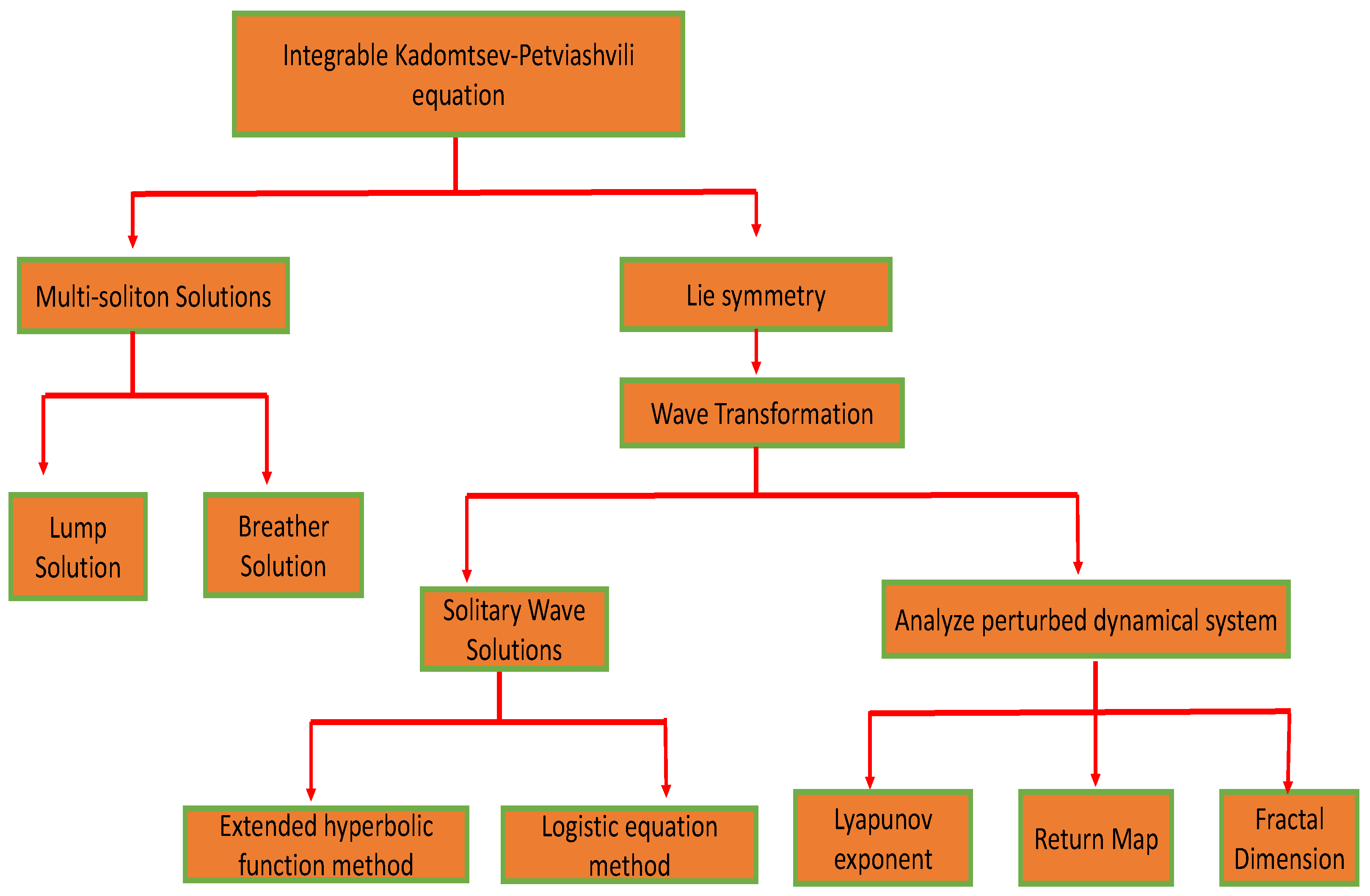
2. Synthesis of Methodologies
2.1. An Overview of the Extended Hyperbolic Function Method
2.2. A Description of the Generalized Logistic Equation Methodology
3. Hirota’s Bilinear Approach
3.1. Lump Solitons of Equation (5)
3.2. Breather Wave Solutions of Equation (5)
4. Lie Group Analysis Applied to Equation (5)
5. Reduction Techniques and Precise Solutions
5.1. Reduction via Translation Symmetry:
5.2. Translation Symmetry-Based Reduction:
5.3. Applying Translation Symmetry Reduction:
5.4. Applying Translation Symmetry Reduction:
5.5. Applying Translation Symmetry Reduction:
5.6. Applying Translation Symmetry Reduction:
5.7. Symmetry-Based Reduction via Transformation
5.8. Reduction Through a Combination of Translational Symmetries,
5.9. Applying Symmetry for System Reduction
5.10. Reduction Through Merging Translational Asymmetries
5.11. Utilizing for Symmetric System Reduction
5.12. Transformation-Induced Reduction Using Symmetries
5.13. Reduction via a Combination of Translation Symmetries:
6. Solitary Wave Solutions of Equation (5)
6.1. The Implementation of the Extended Hyperbolic Function Technique
6.2. The Adoption of the Generalized Logistic Equation Approach
7. The Visual Interpretation of the Solutions
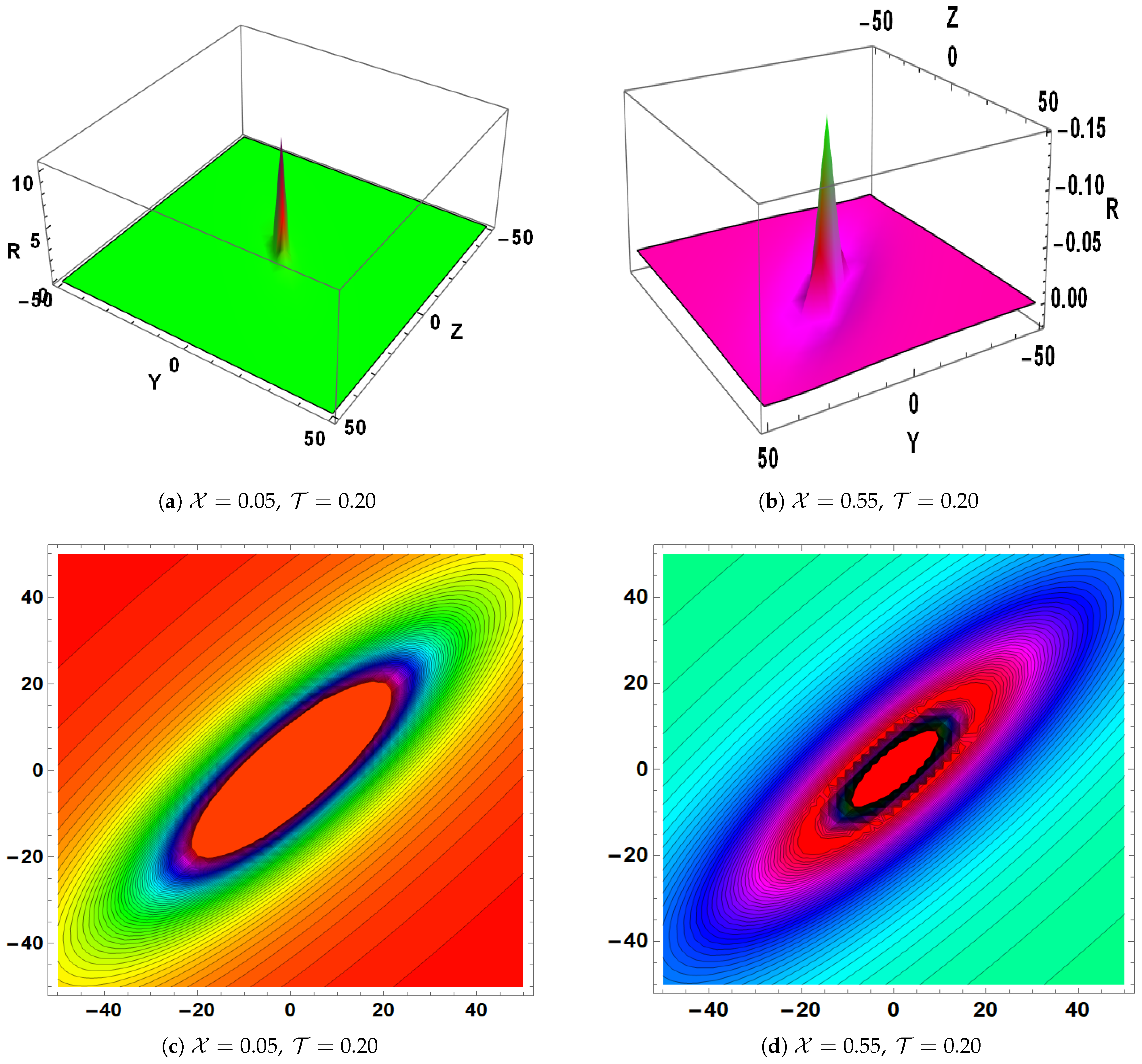
- The lump–periodic soliton characterized by the parameters , , , and is shown for various values of within the domain in Figure 2.
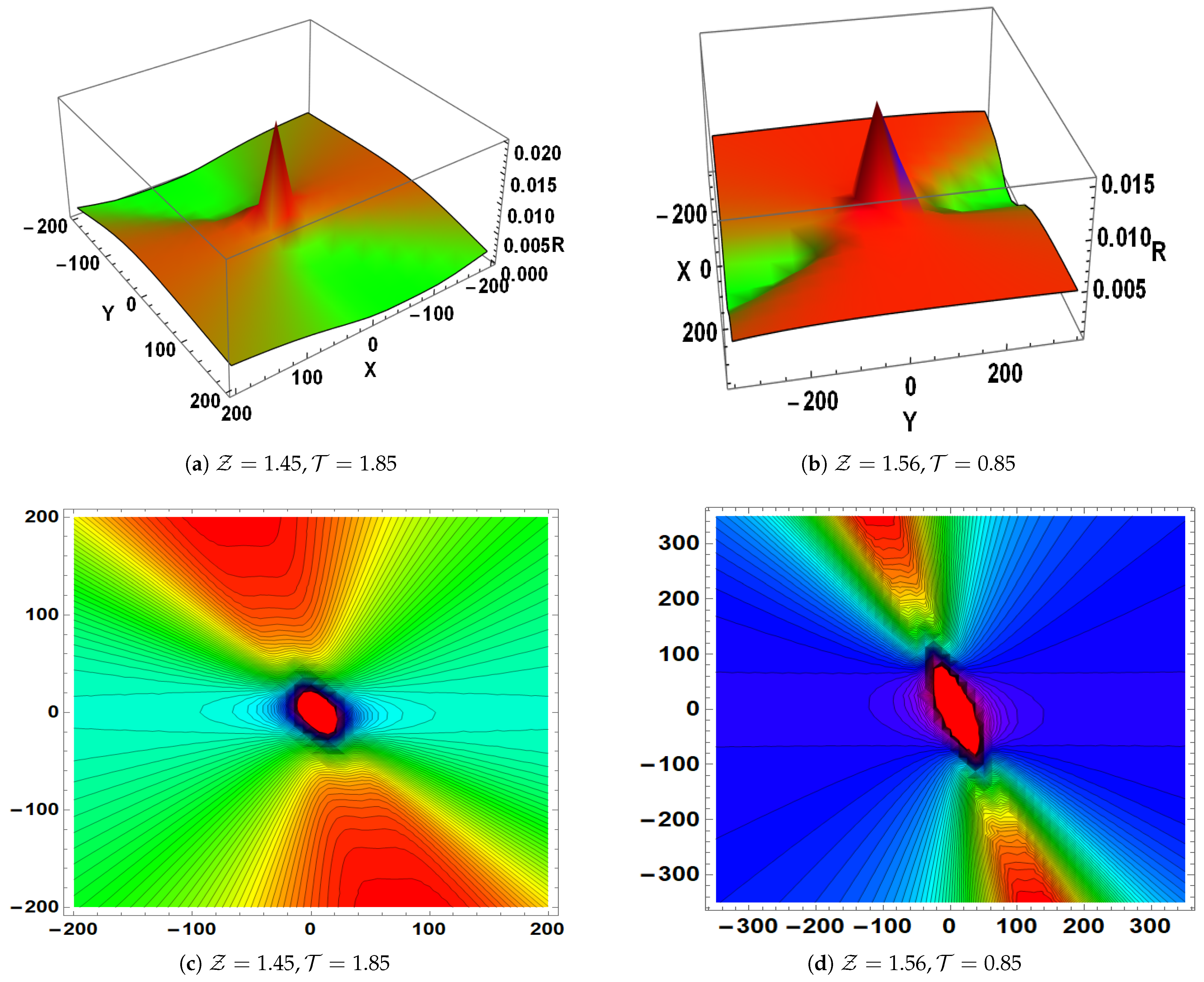
- The lump–periodic soliton characterized by the parameters , , , and is shown for various values of and within the domain in Figure 3.
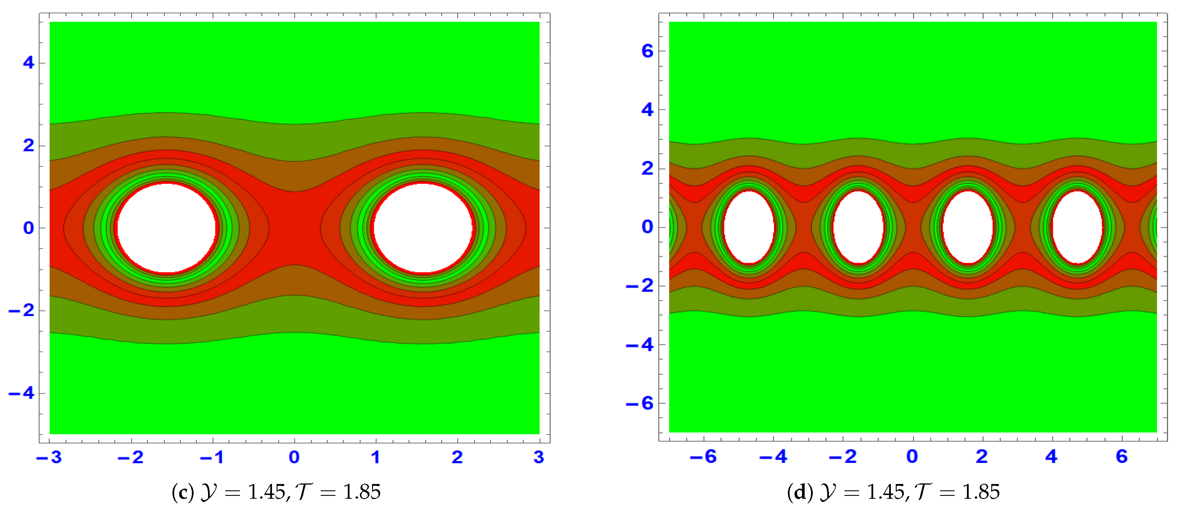
- The breather soliton characterized by the parameters , , , and is shown for various values of and within the domain in Figure 4.
- The breather soliton characterized by the parameters , , , and is shown for various values of and within the domain in Figure 5.
- In the study of PDEs, especially in nonlinear wave dynamics, lump and breather solutions are important. Lump solutions are important for modeling stable, non-dispersive waveforms in fluid dynamics, plasma physics, and optical fiber communications because they are localized, logically decaying structures that explain solitonic behaviors without singularities. Conversely, breather solutions are essential for characterizing wave propagation in nonlinear lattices, Bose–Einstein condensates, and mechanical systems because they describe periodic or localized oscillatory waves with concentrated energy. They can be used to comprehend nonlinear interactions in complicated media, create rogue waves, and create optical solitons.
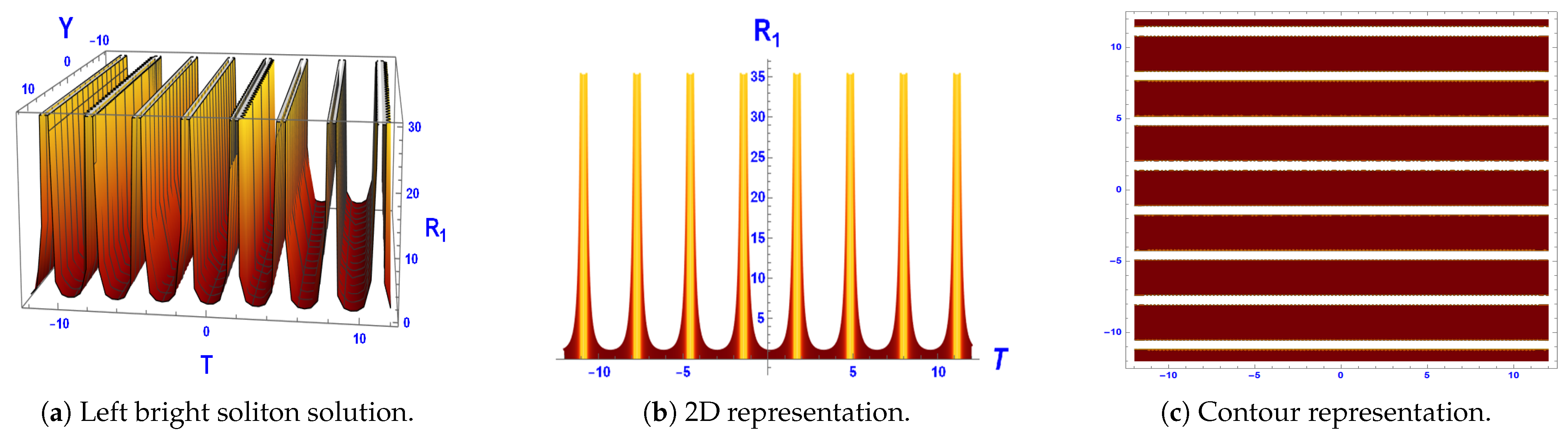
- Figure 6: This graph illustrates that the proposed model exhibits a trigonometric solution, as described by Equation (101). When the parameters are set to , , , , , and , with a positive wave speed of 3, the solution forms a family of periodic singular solitons as shown in Figure 6a–c. The solution is defined over the domain . When modeling intricate wave patterns in nonlinear systems, periodic singular solitons are essential because they provide information on stability transitions and bifurcations. They are useful in fields where the comprehension of wave behavior is crucial, such as fluid dynamics, plasma physics, and optical fiber communications. These solitons aid in the mathematical study of partial differential equations’ compatibility, chaos, and multistability. In many branches of science and technology, the evaluation of them aids in the prediction and management of nonlinear wave occurrences [33,34].
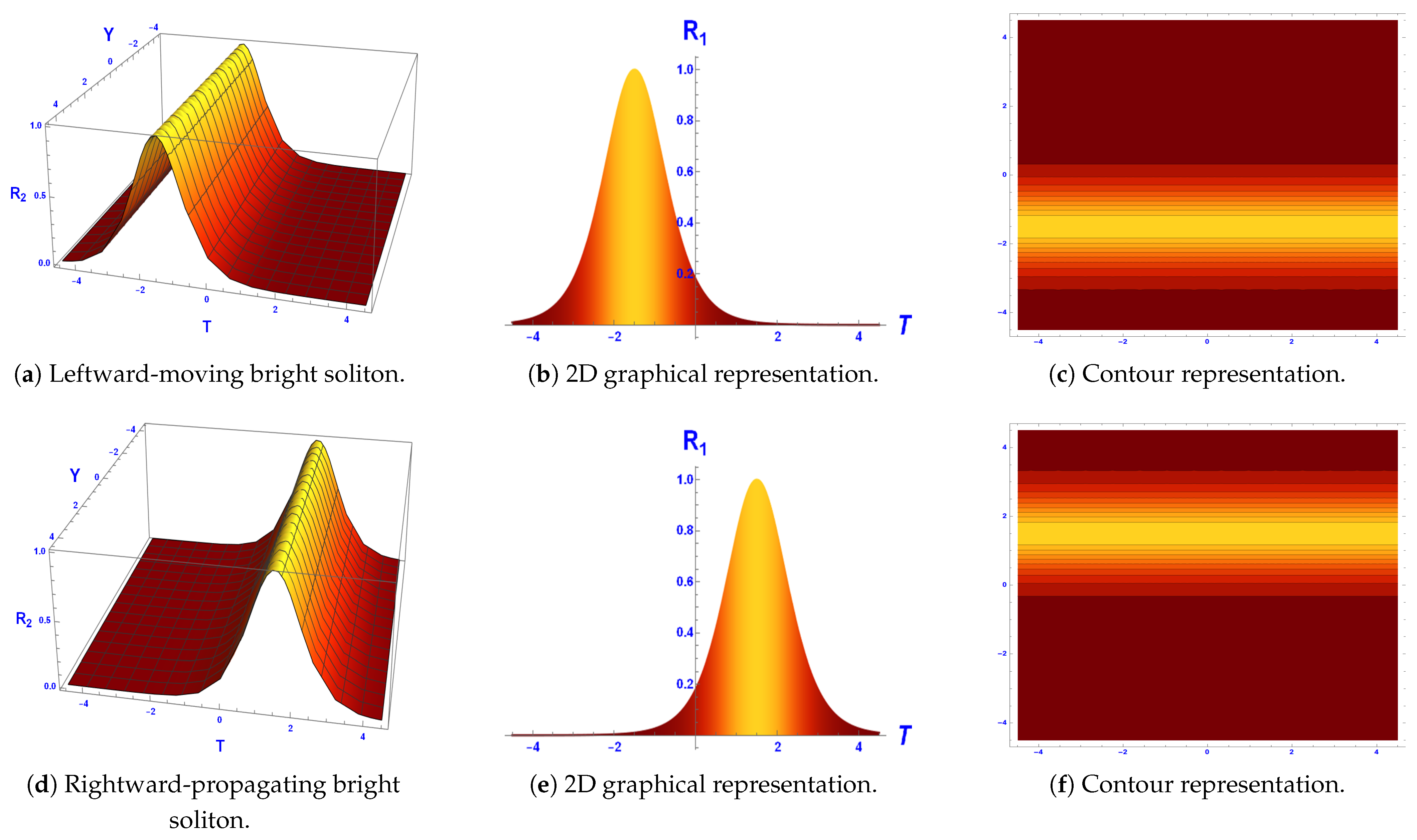
- Figure 7: This plot illustrates that the model possesses a hyperbolic solution, as given by Equation (102). With the parameter values of , , , , , and and a wave speed of 2, a leftward-moving bright soliton solution emerges within the domain , as shown in Figure 7a–c. If the wave speed is changed to −2, the bright soliton reverses direction, moving rightward instead as shown in Figure 7d–f. Moreover, as the domain range expands, the bright soliton transitions into a singular soliton solution. Bright soliton solutions that move left and right are essential for comprehending the transmission of waves and energy transport in nonlinear media. They are extensively used in the study of fluid dynamics, plasma waves, and optical fiber interactions, where directional wave movement affects interactions and stability. Signal processing and information transfer in optical and quantum systems depend on the capacity to control the soliton direction by varying the wave speed. Furthermore, their domain expansion-induced transition into single solitons provides insights into turbulence, rogue waves, and wave collapse [35,36].
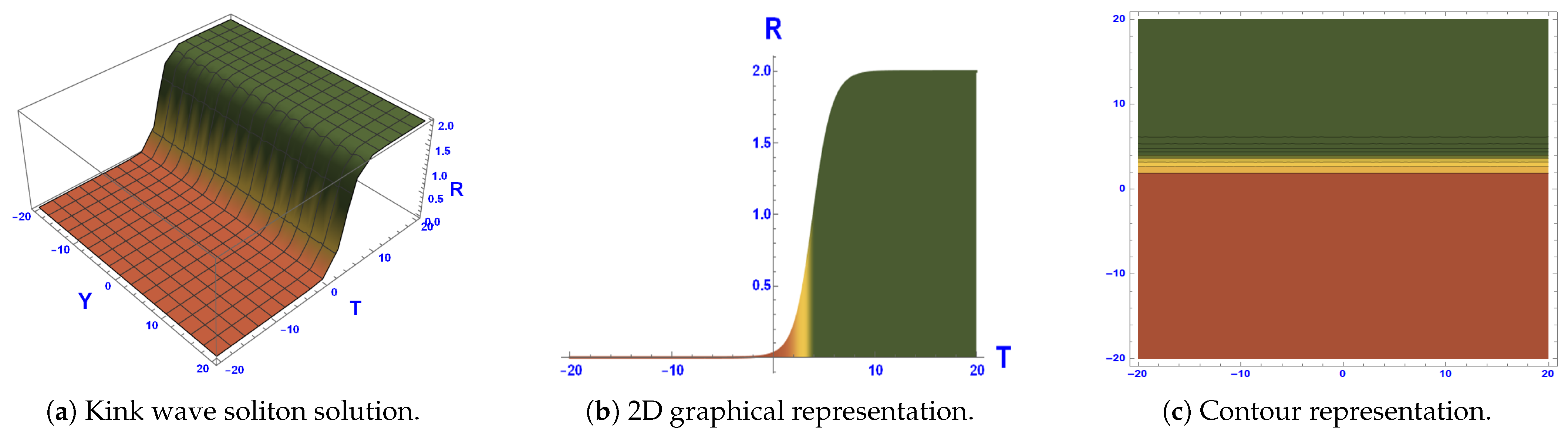
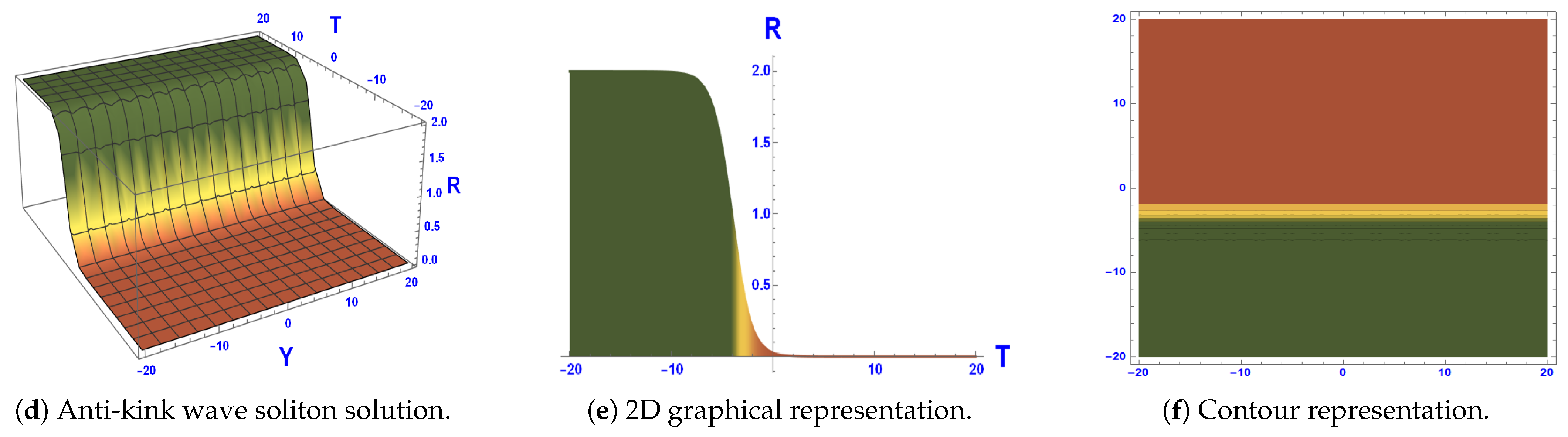
- Figure 7: This graph illustrates that the model possesses an exponential solution, as given by Equation (110). With the parameter values of , , , , , , , and and a wave speed of 1.23, a kink soliton solution emerges within the domain , as shown in Figure 8a–c. If the wave speed is changed to −1.23, the anti-kink soliton reverses direction, moving rightward instead as shown in Figure 8d–f. The phase shifts, domain borders, and energy transfer in nonlinear systems—especially in condensed matter physics and field theory—are all described by kink soliton solutions. In fields like optical fibers and plasma physics, where information transfer depends on steady wave propagation, they are essential. In complicated nonlinear media, anti-kink brilliant soliton solutions aid in the analysis of stability, collision dynamics, and wave collisions. They are used to describe shock waves, brain impulses, and early universe structures in cosmological theory, organisms, and fluid motion.
8. Chaotic Behavior
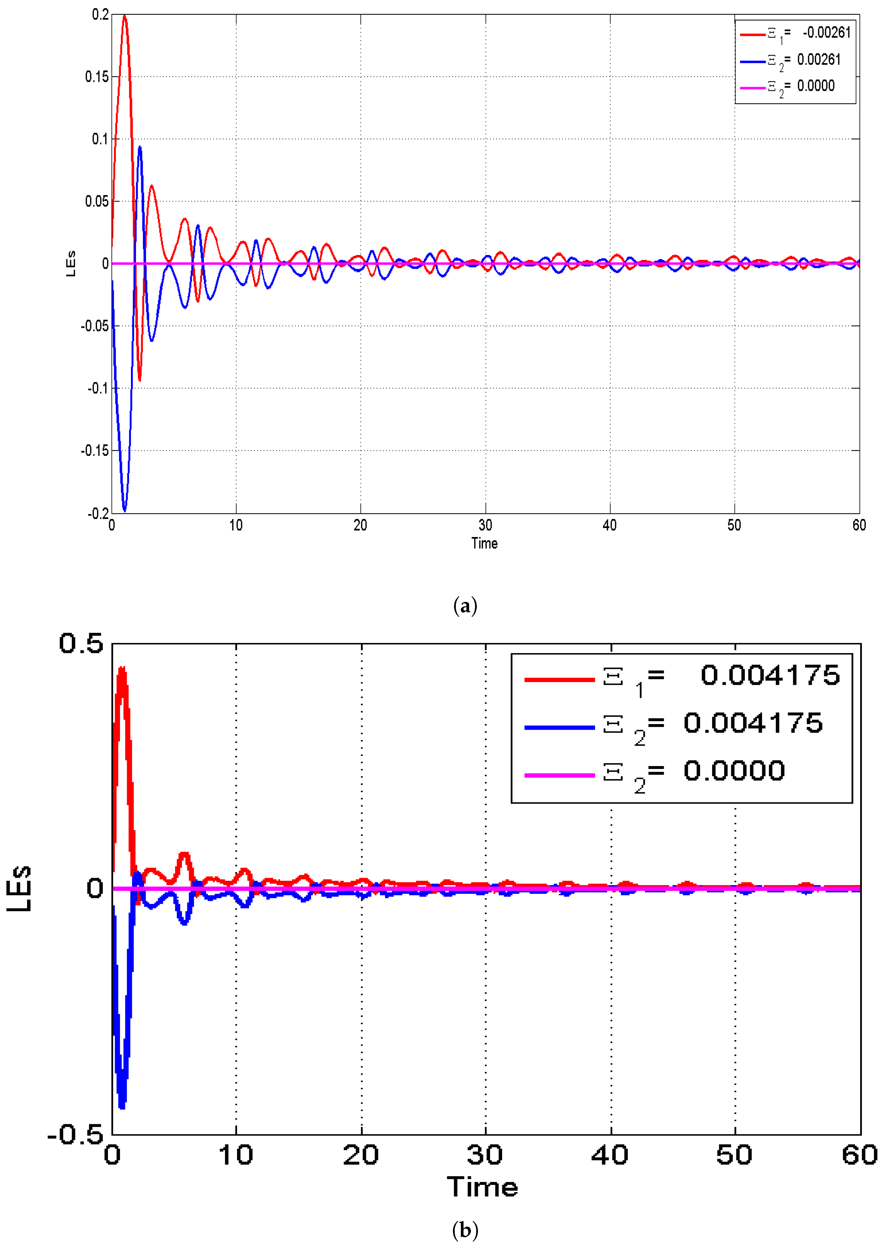
8.1. Lyapunov Exponent
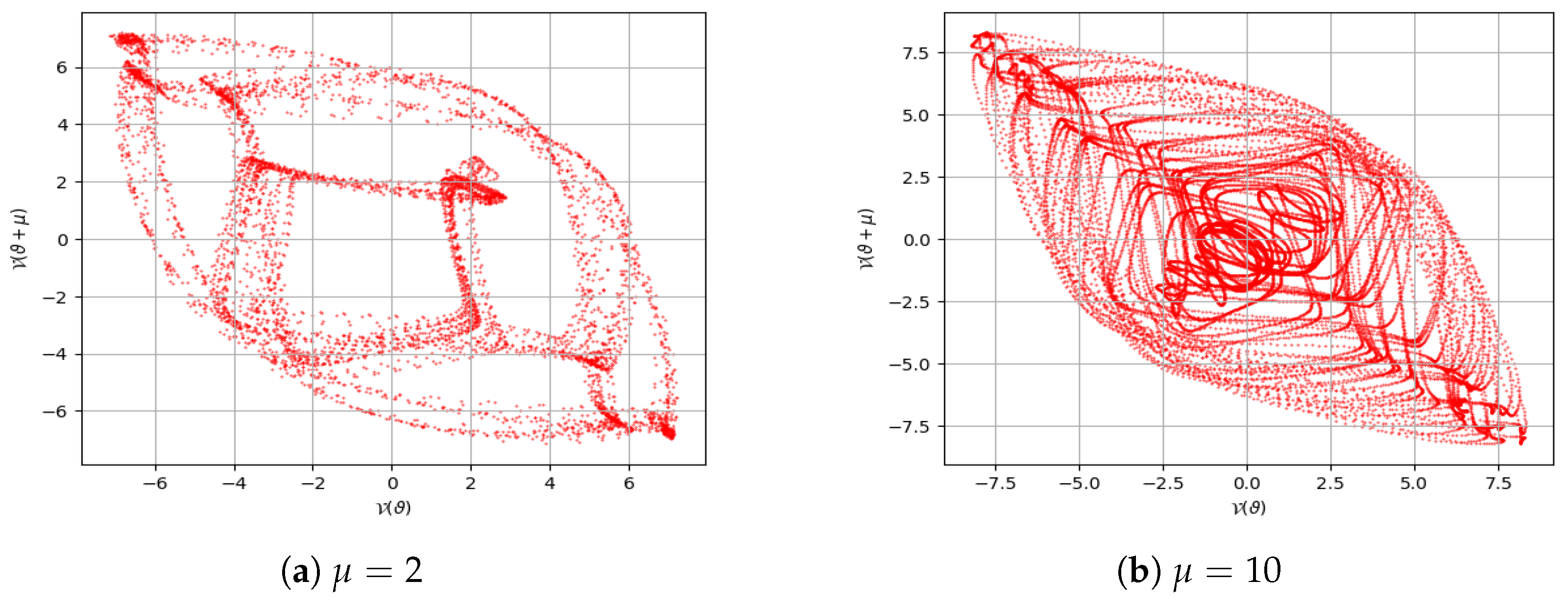
8.2. Return Maps
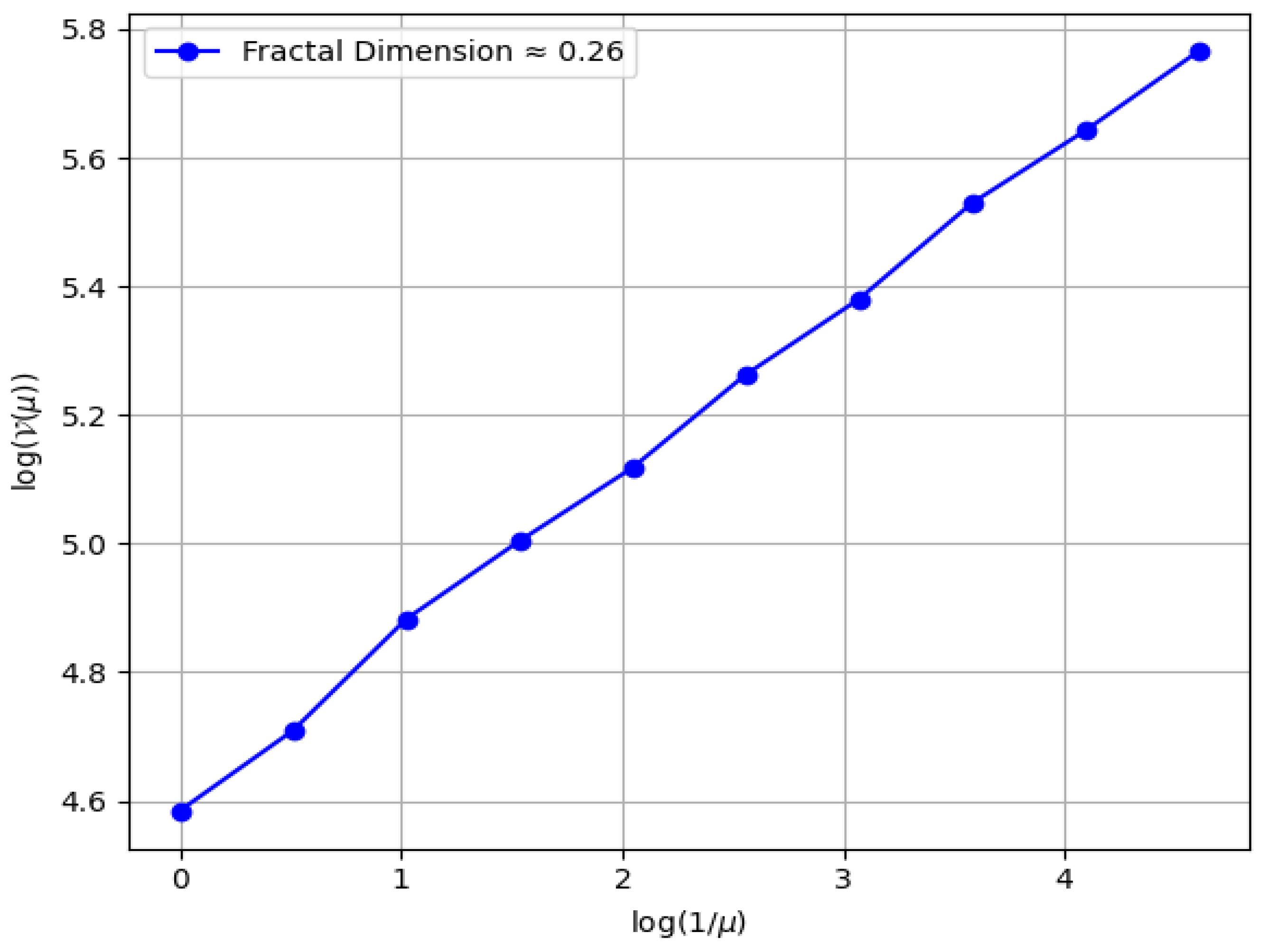
8.3. Fractal Dimension
9. Conclusions
Author Contributions
Funding
Data Availability Statement
Acknowledgments
Conflicts of Interest
Abbreviations
| KP | Kadomtsev–Petviashvili |
| NLPDEs | Nonlinear partial differential equations |
References
- Treves, F. Applications of distributions to PDE theory. Am. Math. Mon. 1970, 77, 241–248. [Google Scholar] [CrossRef]
- Kazdan, J.L. Applications of partial differential equations to problems in geometry. Grad. Texts Math. 1983. Available online: https://www2.math.upenn.edu/~kazdan/japan/japan.pdf (accessed on 28 April 2025).
- Faridi, W.A.; Bakar, M.A.; Akgül, A.; Abd El-Rahman, M.; El Din, S.M. Exact fractional soliton solutions of thin-film ferroelectric material equation by analytical approaches. Alex. Eng. J. 2023, 78, 483–497. [Google Scholar] [CrossRef]
- Niwas, M.; Kumar, S.; Rajput, R.; Chadha, D. Exploring localized waves and different dynamics of solitons in (2+1)-dimensional Hirota bilinear equation: A multivariate generalized exponential rational integral function approach. Nonlinear Dyn. 2024, 112, 9431–9444. [Google Scholar] [CrossRef]
- Younas, U.; Hussain, E.; Muhammad, J.; Sharaf, M.; Meligy, M.E. Chaotic Structure, Sensitivity Analysis and Dynamics of Solitons to the Nonlinear Fractional Longitudinal Wave Equation. Int. J. Theor. Phys. 2025, 64, 42. [Google Scholar] [CrossRef]
- Dong, S.H. A new approach to the relativistic Schrödinger equation with central potential: Ansatz method. Int. J. Theor. Phys. 2001, 40, 559–567. [Google Scholar] [CrossRef]
- Riaz, M.B.; Jhangeer, A.; Martinovic, J.; Kazmi, S.S. Bifurcation and chaos: Unraveling soliton solutions in a couple fractional-order nonlinear evolution equation. Nonlinear Eng. 2024, 13, 20240024. [Google Scholar] [CrossRef]
- Hirota, R. Direct methods in soliton theory. In Solitons; Springer: Berlin/Heidelberg, Germany, 1980; pp. 157–176. [Google Scholar]
- Shang, Y.; Huang, Y.; Yuan, W. The extended hyperbolic functions method and new exact solutions to the Zakharov equations. Appl. Math. Comput. 2008, 200, 110–122. [Google Scholar] [CrossRef]
- Farooq, K.; Hussain, E.; Younas, U.; Mukalazi, H.; Khalaf, T.M.; Mutlib, A.; Shah, S.A.A. Exploring the wave’s structures to the nonlinear coupled system arising in surface geometry. Sci. Rep. 2025, 15, 11624. [Google Scholar] [CrossRef]
- Sait, A.; Altunay, R. Abundant travelling wave solutions of (3 + 1) dimensional Boussinesq equation with dual dispersion. Rev. Mex. Física E 2022, 19, 0202031. [Google Scholar]
- Ablowitz, M.J.; Clarkson, P.A. Solitons, Nonlinear Evolution Equations and Inverse Scattering; Cambridge University Press: Cambridge, UK, 1991; Volume 149. [Google Scholar]
- Matveev, V.B.; Salle, M.A. Darboux Transformations and Solitons; Springer Series in Nonlinear Dynamics; Springer: Berlin/Heidelberg, Germany, 1991. [Google Scholar]
- Liu, J.G.; Yang, X.J.; Feng, Y.Y. Characteristic of the algebraic solitary wave solutions for two extended (2 + 1)-dimensional Kadomtsev–Petviashvili equations. Mod. Phys. Lett. A 2020, 35, 2050028. [Google Scholar] [CrossRef]
- Xu, Y.; Zheng, X.; Xin, J. New explicit and exact solitary wave solutions of (3 + 1)-dimensional KP equation. Math. Found. Comput. 2021, 4, 105–115. [Google Scholar] [CrossRef]
- Liu, J.G.; Yang, X.J.; Feng, Y.Y.; Cui, P. Nonlinear dynamic behaviors of the generalized (3 + 1)-dimensional KP equation. ZAMM-J. Appl. Math. Mech. Angew. Math. Mech. 2022, 102, e202000168. [Google Scholar] [CrossRef]
- Ozisik, M.; Secer, A.; Bayram, M.; Yusuf, A.; Sulaiman, T.A. Soliton solutions of the (2 + 1)-dimensional Kadomtsev–Petviashvili equation via two different integration schemes. Int. J. Mod. Phys. B 2023, 37, 2350212. [Google Scholar] [CrossRef]
- Manukure, S.; Zhou, Y.; Ma, W.X. Lump solutions to a (2 + 1)-dimensional extended KP equation. Comput. Math. Appl. 2018, 75, 2414–2419. [Google Scholar] [CrossRef]
- Guo, J.; He, J.; Li, M.; Mihalache, D. Exact solutions with elastic interactions for the (2 + 1)-dimensional extended Kadomtsev–Petviashvili equation. Nonlinear Dyn. 2020, 101, 2413–2422. [Google Scholar] [CrossRef]
- Ma, Y.L.; Wazwaz, A.M.; Li, B.Q. New extended Kadomtsev–Petviashvili equation: Multiple soliton solutions, breather, lump and interaction solutions. Nonlinear Dyn. 2021, 104, 1581–1594. [Google Scholar] [CrossRef]
- Li, L.; Yan, Y.; Xie, Y. Dynamical analysis of rational and semi-rational solution for a new extended (3 + 1)-dimensional Kadomtsev-Petviashvili equation. Math. Methods Appl. Sci. 2023, 46, 1772–1788. [Google Scholar] [CrossRef]
- Nasreen, N.; Yadav, A.; Malik, S.; Hussain, E.; Alsubaie, A.S.; Alsharif, F. Phase trajectories, chaotic behavior, and solitary wave solutions for (3 + 1)-dimensional integrable Kadomtsev–Petviashvili equation in fluid dynamics. Chaos Solitons Fractals 2024, 188, 115588. [Google Scholar] [CrossRef]
- Luo, A.C.; Gazizov, R.K. Symmetries and Applications of Differential Equations; Springer: Singapore, 2021. [Google Scholar]
- Jiwari, R.; Kumar, V.; Karan, R.; Alshomrani, A.S. Haar wavelet quasilinearization approach for MHD Falkner–Skan flow over permeable wall via Lie group method. Int. J. Numer. Methods Heat Fluid Flow 2017, 27, 1332–1350. [Google Scholar] [CrossRef]
- Bluman, G.W.; Cheviakov, A.F.; Anco, S.C. Applications of Symmetry Methods to Partial Differential Equations; Springer: New York, NY, USA, 2010. [Google Scholar] [CrossRef]
- Kumar, S.; Jiwari, R.; Mittal, R.C.; Awrejcewicz, J. Dark and bright soliton solutions and computational modeling of nonlinear regularized long wave model. Nonlinear Dyn. 2021, 104, 661–682. [Google Scholar] [CrossRef]
- Baker, G.L.; Gollub, J.P. Chaotic Dynamics: An Introduction; Cambridge University Press: Cambridge, UK, 1996. [Google Scholar]
- El-Shorbagy, M.A.; Akram, S.; ur Rahman, M. Investigation of lump, breather and multi solitonic wave solutions to fractional nonlinear dynamical model with stability analysis. Partial Differ. Equ. Appl. Math. 2024, 12, 100955. [Google Scholar] [CrossRef]
- Jafari, M.; Zaeim, A.; Gandom, M. On similarity reductions and conservation laws of the two non-linearity term Benjamin-Bona-Mahoney equation. J. Math. Ext. 2023, 17, 1–22. [Google Scholar]
- Jafari, M.; Mahdion, S.; Akgül, A.; Eldin, S.M. New conservation laws of the Boussinesq and generalized Kadomtsev–Petviashvili equations via homotopy operator. Results Phys. 2023, 47, 106369. [Google Scholar] [CrossRef]
- Jafari, M.; Zaeim, A.; Tanhaeivash, A. Symmetry group analysis and conservation laws of the potential modified KdV equation using the scaling method. Int. J. Geom. Methods Mod. Phys. 2022, 19, 2250098. [Google Scholar] [CrossRef]
- Jafari, M.; Mahdion, S. Non-classical symmetry and new exact solutions of the Kudryashov-Sinelshchikov and modified KdV-ZK equations. AUT J. Math. Comput. 2023, 4, 195–203. [Google Scholar]
- Li, B.; Liang, H.; He, Q. Multiple and generic bifurcation analysis of a discrete Hindmarsh-Rose model. Chaos Solitons Fractals 2021, 146, 110856. [Google Scholar] [CrossRef]
- Zhang, X.; Yang, X.; He, Q. Multi-scale systemic risk and spillover networks of commodity markets in the bullish and bearish regimes. N. Am. J. Econ. Financ. 2022, 62, 101766. [Google Scholar] [CrossRef]
- Zhu, X.; Xia, P.; He, Q.; Ni, Z.; Ni, L. Coke price prediction approach based on dense GRU and opposition-based learning salp swarm algorithm. Int. J. Bio-Inspired Comput. 2023, 21, 106–121. [Google Scholar] [CrossRef]
- Eskandari, Z.; Avazzadeh, Z.; Khoshsiar Ghaziani, R.; Li, B. Dynamics and bifurcations of a discrete-time Lotka–Volterra model using nonstandard finite difference discretization method. Math. Methods Appl. Sci. 2022, 48, 7197–7212. [Google Scholar] [CrossRef]
- Mahmood, T.; Alhawael, G.; Akram, S.; ur Rahman, M. Exploring the Lie symmetries, conservation laws, bifurcation analysis and dynamical waveform patterns of diverse exact solution to the Klein–Gordan equation. Opt. Quantum Electron. 2024, 56, 1978. [Google Scholar] [CrossRef]
- Muhammad, J.; Younas, U.; Hussain, E.; Ali, Q.; Sediqmal, M.; Kedzia, K.; Jan, A.Z. Solitary wave solutions and sensitivity analysis to the space-time β-fractional Pochhammer–Chree equation in elastic medium. Sci. Rep. 2024, 14, 28383. [Google Scholar] [CrossRef] [PubMed]
- Barreira, L. Lyapunov Exponents; Springer International Publishing: Cham, Switzerland, 2017; Volume 1002. [Google Scholar]
- Almheidat, M.; Alqudah, M.; Alderremy, A.A.; Elamin, M.; Mahmoud, E.E.; Ahmad, S. Lie-bäcklund symmetry, soliton solutions, chaotic structure and its characteristics of the extended (3 + 1) dimensional Kairat-II model. Nonlinear Dyn. 2025, 113, 2635–2651. [Google Scholar] [CrossRef]
- Theiler, J. Estimating fractal dimension. J. Opt. Soc. Am. A 1990, 7, 1055–1073. [Google Scholar] [CrossRef]


Disclaimer/Publisher’s Note: The statements, opinions and data contained in all publications are solely those of the individual author(s) and contributor(s) and not of MDPI and/or the editor(s). MDPI and/or the editor(s) disclaim responsibility for any injury to people or property resulting from any ideas, methods, instructions or products referred to in the content. |
© 2025 by the authors. Licensee MDPI, Basel, Switzerland. This article is an open access article distributed under the terms and conditions of the Creative Commons Attribution (CC BY) license (https://creativecommons.org/licenses/by/4.0/).
Share and Cite
Beenish; Samreen, M.; Alshammari, F.S. Exploring Solitary Wave Solutions of the Generalized Integrable Kadomtsev–Petviashvili Equation via Lie Symmetry and Hirota’s Bilinear Method. Symmetry 2025, 17, 710. https://doi.org/10.3390/sym17050710
Beenish, Samreen M, Alshammari FS. Exploring Solitary Wave Solutions of the Generalized Integrable Kadomtsev–Petviashvili Equation via Lie Symmetry and Hirota’s Bilinear Method. Symmetry. 2025; 17(5):710. https://doi.org/10.3390/sym17050710
Chicago/Turabian StyleBeenish, Maria Samreen, and Fehaid Salem Alshammari. 2025. "Exploring Solitary Wave Solutions of the Generalized Integrable Kadomtsev–Petviashvili Equation via Lie Symmetry and Hirota’s Bilinear Method" Symmetry 17, no. 5: 710. https://doi.org/10.3390/sym17050710
APA StyleBeenish, Samreen, M., & Alshammari, F. S. (2025). Exploring Solitary Wave Solutions of the Generalized Integrable Kadomtsev–Petviashvili Equation via Lie Symmetry and Hirota’s Bilinear Method. Symmetry, 17(5), 710. https://doi.org/10.3390/sym17050710