Abstract
These notes are an informal overview of techniques related to deformation theory in the context of physics. Beginning from motivation for the concept of a sheaf, they build up through derived functors, resolutions, and the functor of points to the notion of a moduli problem, emphasizing physical motivation and the principles of locality and general covariance at each step. They are primarily aimed at those who have some prior exposure to quantum field theory and are interested in acquiring some intuition or orientation regarding modern mathematical methods. A couple of small things are new, including a discussion of the twist of conformal supergravity in generic backgrounds at the level of the component fields and a computation relating the two-dimensional local cocycle for the Weyl anomaly to the one for the Virasoro anomaly. I hope they will serve as a useful appetizer for the more careful and complete treatments of this material that are already available.
1. Introduction
The main purpose of this article is to give a bird’s-eye view of how ideas from derived deformation theory can serve as a unifying principle in the study of field theories and their symmetries. I will do this in a rather personal, intuitive, and erratic manner, focusing on giving a perspective rather than a full and careful treatment.
The central idea is that field theory is interested in local structures on manifolds, and in their symmetries and deformations. We imagine studying the collection of such structures, together with their (auto)equivalences, on arbitrary geometries of an appropriate class. The resulting package is a moduli problem. If one restricts to thinking perturbatively—studying infinitesimal or formal deformations of a fixed local structure—then the resulting formal moduli problem on any geometry is controlled by a “local Lie algebra” (Definition 4, following ([1], §3.1)) defined there.
This technical language is powerful enough to accommodate essentially all of the structures one encounters in studying a field theory. Numerous specific instances of the necessary technology are well established in the physics community and were, in fact, discovered (or rediscovered) there and developed over the last 50 or more years. To give a few examples, the BRST formalism constructs a derived model for the space of gauge fields with gauge equivalences, while the BV formalism identifies and characterizes the subclass of variational moduli problems; these are (up to subtleties) precisely the ones that are -shifted symplectic [2], reflecting the natural pairing between fields and equations of motion. In parallel with Dirac’s theory of constraints and degenerate systems in quantum mechanics, obvious weakenings of this structure to -shifted presymplectic structures or -shifted Poisson structures are available and arise naturally in non-Lagrangian systems, notably including theories of self-dual higher gauge fields. Symmetries of a field theory amount to couplings of it to another (formal) moduli problem, representing the corresponding collection of backgrounds, and so on.
Despite its power, rigor, and conceptual simplicity, and despite its enthusiastic adoption and further development within several distinct research communities, this general viewpoint seems to have been slow in passing into the typical toolkit of the theoretical physicist. It feels as though the breadth and unity of the perspective has not been as well appreciated as it might. At the least, these ideas have been slow in being absorbed into the standard basic training. There are many reasons for this, beyond inertia, that one might name. The one that feels decisive to me is that many small but distinct intuitions are required to really grasp the central ideas, and that these come from parts of math—especially algebraic geometry and homological algebra—that are farther from young physicists’ bread and butter. Let me permit myself to use a rather long quote from Ravi Vakil’s The Rising Sea ([3], §0.1) to frame this point:
Before discussing details, I want to say clearly at the outset: the wonderful machine of modern algebraic geometry was created to understand basic and naive questions about geometry (broadly construed). The purpose of this book is to give you a thorough foundation in these powerful ideas. Do not be seduced by the lotus-eaters into infatuation with untethered abstraction. Hold tight to your geometric motivation as you learn the formal structures which have proved to be so effective in studying fundamental questions. When introduced to a new idea, always ask why you should care. Do not expect an answer right away, but demand an answer eventually. Try at least to apply any new abstraction to some concrete example you can understand well. See if you can make a rough picture to capture the essence of the idea. (I deliberately asked an uncoordinated and confused three-year-old to make most of the figures in the book in order to show that even quick sketches can enlighten and clarify.)
Understanding algebraic geometry is often thought to be hard because it consists of large complicated pieces of machinery. In fact the opposite is true; to switch metaphors, rather than being narrow and deep, algebraic geometry is shallow but extremely broad. It is built out of a large number of very small parts, in keeping with Grothendieck’s vision of mathematics. It is a challenge to hold the entire organic structure, with its messy interconnections, in your head.
Although Vakil is discussing algebraic geometry, the same could be said, mutatis mutandis, of modern mathematical or theoretical physics, especially in regard to the sorts of example-driven intuitions that are so important there. Perhaps the real root of the accessibility problem for approaches to QFT that draw on the deep and profound connections to patterns of thought in algebraic geometry is that one is dealing with the breadth of both disciplines taken together!
Another issue, which Vakil takes note of in some way, is the unfortunate tendency to paint any “fancy” or “formal” approach to the subject as “unnecessary abstraction”, and the people who reach for it as lotus-eaters. On the contrary! The purpose of all of this discussion is to understand simple things better: to use fewer, more powerful tools, to avoid reinventing the wheel, and to become confused less. Here, I will allow myself to cite Hamilton [4]:
Those who have meditated on the beauty and utility, in theoretical mechanics, of the general method of Lagrange—who have felt the power and dignity of that central dynamical theorem which he deduced, in the Mécanique Analytique, from a combination of the principle of virtual velocities with the principle of d’Alembert—and who have appreciated the simplicity and harmony which he introduced into the research of the planetary perturbations, by the idea of the variation of parameters, and the differentials of the disturbing function, must feel that mathematical optics can only then attain a coordinate rank with mathematical mechanics, or with dynamical astronomy, in beauty, power, and harmony, when it shall possess an appropriate method, and become the unfolding of a central idea.
Mirroring these two quotes, it seems valuable to try and seek out the formal structures that reveal some sort of hidden or emergent unity, lurking in the wide-ranging organic structure that is quantum field theory. To that end, I want to record some general ideas, tools, and patterns of thought that have proved useful and fruitful to me, and which I have picked up over time from various references and (more often) from conversations with many others. In keeping with this, the structure of the text is necessarily fragmented, with a sequence of small metaphors and relatively self-contained attempts at explanation following on one another. A path is formed by laying one stone at a time.
I cannot hope to compete with the thorough and foundational treatments of this material that already exist. Here, Costello and Gwilliam’s books [1,5], from which much of the perspective springs, deserve special note, as do the treatments in the two-volume IAS collection on “Quantum Fields and Strings” (of which I will cite certain portions throughout the text) and various other pieces of writing by Dan Freed [6,7,8]. My intended audience consists of students who have had some exposure to quantum field theory, who find the more formal corners of the literature interesting, and who are looking to orient themselves or collect some informal intuition. I hope this article will give them a jumping-off point for a more serious engagement with the literature. With luck, it may also serve as amusing bathroom reading for one or two experts.
The following portions of the article might be regarded as new: In Section 7, as an illustration of the way that twisting connects supersymmetric theories to holomorphic ones, I provide a computation of the holomorphic twist of the four-dimensional conformal supergravity multiplet. (At the level of currents, this is the universal stress tensor multiplet for an superconformal theory.) The computation works at the abelian level, but starting with any generic superconformal structure compatible with a holomorphic twist; such background independence is a pleasing feature, and it is nice to see in detail that only the conformal structure, rather than some choice of metric, appears at every stage. In Section 5.6, I extract the local cocycle representing the Virasoro algebra from the complexified two-dimensional a-type conformal anomaly; the result is a matter of common knowledge, but I was unable to find an explicit computation written out. Lastly, I allow myself to engage in a bit of speculation about the absence of global symmetries in “complete” theories in §6.3.4.
Throughout, I will use names and bits of terminology that may be unfamiliar. The purpose is neither to weigh down the text, nor to intimidate the reader! Rather, I hope to show that nothing too intimidating is hidden behind these names, and to try and give a quick sketch (in the manner of an uncoordinated three-year-old) that will indicate the idea the terminology is meant to convey—or better yet, the intuitive picture it should conjure up.
1.1. How to Read This Article
Here is a rough roadmap:
- §1:
- Introduction. Self-explanatory, and hopefully also explanatory in a broader way.
- §2:
- Physicists should have invented sheaves. By thinking about the principle of general covariance, we arrive (in a massively simplified setting) at the notion of an “étale site:” a category of structured manifolds, related by maps that are locally structure-preserving isomorphisms. By thinking about local fields, we arrive at the notion of a sheaf on this site.
- §3:
- Subtle objects are best built from boring ones. By using a system of local observers to reconstruct global information, we rediscover Čech cohomology. Thinking about local equations of motion as a source of propagation of information, we rediscover de Rham cohomology and the equivalence between the two. Taken together, the two examples illustrate the basic ideas of resolutions and derived functors.
- §4:
- Lie algebras model nonlinearities, infinitesimally. We sketch the central dogma of derived deformation theory, where differential graded (or dg) Lie algebras play, in some sense, the role of resolutions. On the way, we give brief, physics-motivated introductions to the spectrum, the functor of points, and other basic intuitions from algebraic geometry, at a cocktail-party level. The main point is to arrive at the definition of the central object, a local Lie algebra. All technical details are omitted.
- §5:
- A field guide to useful local Lie algebras. We list a bunch of useful examples of local Lie algebras, representing both typical building blocks of field theories and central examples of symmetries. Self-dual fields, spacetime symmetries, and holomorphic symmetries are included, the latter encompassing “higher” Virasoro and Kac–Moody algebras in arbitrary complex dimension.
- §6:
- Current algebras. This is essentially a discussion of the factorization-algebra enhancement of Noether’s theorem proved by Costello and Gwilliam, but it leads to ideas related to Koszul duality, a well-intentioned screed on terminology, some discussion of the operation of gauging, and a bit of ill-advised speculation.
- §7:
- Higher Virasoro algebras in theories. We give an explicit computation of the holomorphic twist of the moduli problem of four-dimensional superconformal structures, obtaining the moduli problem of complex structures on a locally conformally Kähler manifold and, thus, the higher Virasoro algebra. While the result is known [9], the computation is nevertheless illuminating.
1.2. Key Notation and Terminology
For the reader’s convenience, we provide a list of key terms and notational habits, together with some pointers to relevant sections of the text:
- Manifolds are always smooth and oriented; they are usually denoted by M and have dimension d.
- Vector bundles over M are usually denoted by an uppercase Roman letter, such as E.
- Categories (§2.1.3) are denoted by a suggestive name in sans-serif type (e.g., ).
- Groupoids (§2.2.5) are categories in which every map is invertible.
- Sheaves (Section 2.2) are denoted by a calligraphic letter (possibly followed by other letters), and will be used for the sections of a bundle E. An underlined object, as in , denotes the locally constant sheaf with that value.
- (Cochain) complexes are collections of objects indexed (“graded”) by the integers. The grading will be written as a superscript. The total object is defined as the direct sum of its graded components, which exists in any category of objects in which we will consider complexes. Total objects are denoted with a bullet: thus, for example,A complex is usually equipped with a differential, which is a self-map d of the complex of degree , satisfying . Somewhat abusively, the differential in a “complex of vector bundles” may be a differential operator on sections.
- Differential forms are denoted by , and carry the exterior derivative (de Rham differential). They are a sheaf of cochain complexes.
- Densities on a manifold form a sheaf, denoted . The sections of this sheaf can be integrated to produce a number, assuming the integral converges. A density is a top form, twisted by the orientation line bundle; since we assume a choice of orientation for expository purposes, . The Lagrangian is a density.
- Lie algebras will be denoted, as usual, by Fraktur letters like . However, a local Lie algebra—which is a cochain complex of bundles, equipped with a Lie bracket on sections—will be denoted by a sheaf-type letter, usually .
- Tensor products of infinite-dimensional vector spaces are completed tensor products in an appropriate well-behaved category. Such technical details are beyond the scope of this informal note; we pass over them in silence and refer to [1,5].
1.3. Acknowledgements
First thanks are due to Ivano Basile, for his work in putting together the special issue of Symmetry in which this article is due to appear, for his kindness in inviting me to contribute, and—beyond that—for many illuminating and enjoyable conversations about physics. I also thank both Ivano and Symmetry for their patience with the preparation of this manuscript, and apologize to them both for my rather boundless abuse of it.
Over the years, my perspectives have been strongly shaped by ongoing conversations with many people, notably including I. Brunner, M. Cederwall, K. Costello, C. Elliott, J. Huerta, S. Gukov, O. Gwilliam, F. Hahner, Si Li, S. Raghavendran, J. Walcher, and (last but not least) B. R. Williams. Language being a virus, I am sure that each of them will see many ideas of their own reflected here, continuing to mutate.
As this work was beginning to take shape, I held lectures at the 2024 Saalburg summer school in Bayrischzell and then delivered a lecture course on “Physics and Geometry” in Munich in the winter semester 2024/25. Notes on the former were prepared by Elden Loomes, Rui Xian Siew, Bartlomiej Sikorski, and Justin Tan; Simon Bukovsek and William Luciani wrote up a script for the latter. I thank them for their hard work in doing so, and also thank the participants of both courses for the chance to hash out some of the intuitive explanations that appear in brief form here. I hope very much that portions of what appears here will be a useful complement to those sets of notes once they appear. I am also grateful to Simon Langenscheidt, who read through a version of the draft and offered helpful suggestions.
I thank the Institut Mittag-Leffler and the organizers of the program “Cohomological aspects of quantum field theory” for hospitality while this work was being prepared, and especially Maxim Zabzine for his help in putting the visit together. Gratitude for further hospitality is due to the Max-Planck-Institut für Mathematik and to the University of Vienna. I also thank the physics department of the LMU München for their support with the Habilitationsprojekt of which this article represents a part. This work is funded by the Deutsche Forschungsgemeinschaft (DFG, German Research Foundation) under Projektnummer 517493862 (Homologische Algebra der Supersymmetrie: Lokalität, Unitarität, Dualität), and further by the Free State of Bavaria.
2. A Field Theory as a Sheaf of Spaces
2.1. General Covariance
We consider the relationship between a field theory and the class of spacetimes on which it can be defined abstractly. This leads us intuitively to a valuable way of codifying the structure of such a class of spacetimes.
- 2.1.1. Cartoons of field theories. When one thinks about a semiclassical field theory, the typical package of structures that one has in mind is something like the following:
- 1:
- One first defines a class of spacetime geometries. In essentially every example, these are taken to be smooth manifolds of a fixed dimension d, equipped with all additional geometric data on which the field theory will depend. Among the most important examples are spin structures, (pseudo-)Riemannian metrics, conformal structures, and complex structures.
- 2:
- To each spacetime geometry M, one associates a space of fields , which is often the space of sections of some chosen natural vector bundle. But could also include connections (in gauge theory), maps to some fixed target manifold X (in sigma models), or metrics (in gravity). The space of fields is graded by ; the grading indicates whether the fields are bosons or fermions.
- 3:
- There is a local Lagrangian density, which is a functional , assigning a top form (or, more properly, density) on the spacetime to each possible field configuration in an appropriately local manner. The action functional of the theory isThe choice of action functional identifies a subspace of on-shell fields, which is the critical locus of the action functional, .
- 4:
- If the action functional is degenerate, there are nontrivial differential relations (sometimes called “Gauss law constraints” or “Bianchi identities”) between the equations of motion defining , so that we do not get a well-defined boundary value problem. Noether’s second theorem relates these identities to the action of local gauge symmetries on , preserving S. We then pass to the quotient, so that the space we are physically interested in is(Sometimes, we do this in the opposite order, first identifying the gauge group and then demanding gauge invariance of the action.)
I imagine that most readers who have worked with Lagrangian field theories will see how their intuitions can be made to conform, at least roughly, to this cartoon. Readers who are curious about “non-Lagrangian” field theories are asked to be patient for a few more pages.
- 2.1.2. The reader may object that I am calling such theories “semiclassical”. Every maneuver described above is purely about classical field theory, so why “semi”? The answer has to do with the requirement that the theory is variational. It would have been possible to describe a broader class of field theories, just described by the solution spaces of natural systems of PDEs on the manifold M. But there is no clear way to talk about what the quantization of such a theory should be; that data are encoded, roughly speaking, by the Poisson bracket, whose existence is guaranteed for variational problems. If one wants, one can imagine that generic Newtonian mechanics is classical, but that Lagrangian or Hamiltonian mechanics is semiclassical. We will return to this point later.
- 2.1.3. It is instructive to put this cartoon into a slightly more structured setting. In doing this, I will freely allow myself to use the terminology of categories and functors, but the only deep purpose of this is as a philosophical reminder: One should always ask oneself about the maps!
It is entirely sufficient for the reader to remember that a category is a collection of objects, a set of morphisms between each pair of objects, and a composition law
that specifies how morphisms concatenate. Note that an object need not be a set, and a morphism need not be any kind of function between sets! A functor is a map of categories: it sends objects to objects and morphisms to morphisms in a way that is compatible with composition. A functor is covariant if it preserves the direction of arrows, and contravariant if it reverses them. The reader interested in more detail is referred to [10]; for an intuitive discussion of some other appearances of categories in physics, one might seek out [11]. We will denote categories with their (abbreviated) names in sans-serif type: , for example.
- 2.1.4. So what maps are appropriate here? The most obvious ones have to do with the fact that fields are locally defined. If is an open subset of some spacetime manifold, and we choose a solution to the equations of motion over M, we can restrict it to N and get a solution to the equations of motion there. So, there should be a restriction map from to and, correspondingly, from to (since we can also restrict an off-shell field configuration). The condition of openness can be thought of as asking that each point has a typical-looking infinitesimal neighborhood; there are no boundaries to deal with.
Another natural class has to do with the principle of relativity, which (in essence) says that physics should be associated to geometric structures of the kind we identified above, rather than to some specific observer or system of coordinates. So, any time we have an isomorphism f between two spacetimes M and that preserves all geometric structures, we should get an isomorphism between and and, similarly, for . In the case where the geometric data are a Lorentzian metric and M is Minkowski space, for example, these data give us a representation of the Poincaré group on the space of fields for which the action is invariant.
- 2.1.5. Open embeddings. In fact, these two examples fit together into a single notion. Given some class of smooth, d-dimensional spacetime manifolds equipped with geometric structures as above, a smooth, structure-preserving map is called an open embedding if
- its image is an open subset;
- f is injective. (So f carries N isomorphically onto its image.)
Note that the condition of being structure-preserving and the open embedding condition are independent. It is clear that any open embedding factors into a pair of an isomorphism of N onto , followed by the inclusion . So open embeddings capture both the kinds of maps we identified physically above.
- 2.1.6. Local equivalences. We are working towards identifying an appropriate category that models spacetimes, together with maps that describe local equivalences between spacetimes. (The reader will hopefully recognize this as a more coordinate-free form of the principle of general covariance.) Open embeddings are essentially the right notion, but we will, in fact, work with a slight generalization, motivated by the desire for full locality:
Definition 1.
A (structure-preserving) map of smooth manifolds is called étale if each point has an open neighborhood U such that is an open embedding. Put differently, f is a local diffeomorphism (and preserves all other relevant structure).
The (structured) étale site is the category whose objects are smooth d-manifolds, equipped with some set of geometric structures as above, and whose morphisms are structure-preserving étale maps: local equivalences of structured manifolds.
We may sometimes indicate the dimension and the structure in the notation for emphasis: for Riemannian d-manifolds, for example. For a good and relevant reference (on other related topics) where this definition is used, see [12]. We remark that this approach—though we have motivated it physically here—generalizes nicely to spaces other than smooth manifolds and, in particular, to much more sophisticated algebraic settings, which is where the term “étale” normally occurs. For a survey at that level of generality, we refer to [13]. If the reader is so inclined, they may think of as an acronym for “spéce-time”, as long as they do not do so in public.
A typical example of an étale morphism that is not an open embedding is the covering map , or any other covering map. So working with étale morphisms ensures that we know how to think of field configurations on as periodic field configurations on . We think of the structured étale site as specifying the natural setting in which a particular d-dimensional field theory lives.
- 2.1.7. Having understood this, we can extend our cartoon from above so as to include both relativistic invariance and locality at the same time:
- 5:
- The assignmentshould define a contravariant functor from the structured étale site to spaces.
- To any spacetime M, the functor assigns the space of on-shell field configurations on M modulo gauge transformations; the action of the functor on morphisms encodes the restriction of fields and also spacetime symmetries, as explained above. Such a functor is called a presheaf.
Our cartoon still needs a bit of refinement. Intuitively, we want it to be true that a set of locally defined field configurations on regions in spacetime that agree on all overlaps glue together into a uniquely defined global field configuration on . (This captures the notion that all observations of the field can be performed by a system of local observers.) This will lead us to the definition of a sheaf.
Secondly, we have not yet specified what we mean by “spaces”. We should be a bit more careful about the target category of our functor. At the end of all this lengthy motivational discussion, we will arrive at a fairly standard definition; see ([8], Definition 3.1) for a recent instance, [7] for some illuminating discussion, or [5] for a careful foundational treatment in the perturbative setting.
- 2.1.8. An example of a field theory. An instructive and relatively uncomplicated example of a field theory in this framework is provided by thinking about a single classical particle moving in the flat n-dimensional space . We emphasize that we are thinking of this theory as a one-dimensional field theory. In general in such formalisms, the degrees of freedom are fields; the parameters labeling points at which those fields can be measured are coordinates on the “spacetime”. In the standard mechanics (whether classical or quantum) of a single particle, the spatial coordinates are physical degrees of freedom that can be measured at any moment in time; the “spacetime”, thus, consists purely of a one-dimensional timeline, whereas the spatial coordinates are promoted to fields.
The additional structure on spacetime consists of a Lorentzian metric; in one dimension, such a metric is equivalent to a volume element that allows us to measure time, or to a preferred real coordinate t, determined up to shifts of the origin. The space of solutions to the equations of motion is the space of functions that are linear in the preferred coordinate: They solve the familiar equation of motion . There are no gauge invariances. A linear function is parameterized by its first two Taylor coefficients at any point, so our functor satisfies
for any connected open interval . Since any linear function on an open interval extends uniquely to a linear function on a larger open interval, we find that our sheaf of spaces is in fact locally constant: Tt assigns the (covariant) phase space of the particle to any connected interval of time.
- 2.1.9. Examples of structures on spacetime. For later use, let us just list some of the most common examples of spacetimes here. The reader is free to ignore any example that feels unfamiliar, at least for the time being.
- 1:
- There is a site of smooth d-dimensional manifolds without any additional structure; its local equivalences are just local diffeomorphisms. A topological field theory is a field theory defined on this site.
- 2:
- If we consider smooth d-manifolds equipped with conformal structures, with local equivalences given by smooth, locally bijective conformal maps, we obtain a site . A conformal field theory is a field theory defined here.
- 3:
- There is a site whose objects are smooth d-manifolds equipped with Riemannian metrics, and whose local equivalences are local isometries. A Euclidean field theory is a field theory defined on this site. Lorentzian field theories are defined analogously, and additional data such as a choice of spin structure can be included in obvious fashion. We emphasize that a Riemannian structure can be profitably thought of as a conformal structure together with a choice of volume form.
- 4:
- We can consider spacetimes that are smooth manifolds of even dimension , equipped with a choice of complex structure. Local equivalences are given by local biholomorphisms. This defines a site of complex n-manifolds; a holomorphic field theory is a field theory defined here.
- Recall that a smooth supermanifold is a smooth d-manifold, equipped with a sheaf of commutative algebras that can locally be identified with a finitely generated exterior algebra (say on k generators) over the smooth functions. A superconformal structure consists, speaking roughly, of a local frame of odd vector fields whose torsion reproduces the structure constants of the supertranslation algebra of flat space. We direct the reader to ([14], chapter 5, §7) for an enlightening early treatment, or to ([9], §2.1.6) for the precise definition we choose to work with. A superconformal structure is the minimal piece of geometric data on which a supersymmetric field theory depends.
- 5:
- There is a site of smooth supermanifolds equipped with a superconformal structure of type . A superconformal field theory is a field theory defined here.
- 6:
- One can also consider sites of smooth supermanifolds equipped with a superconformal structure and additional geometric data. Typically, the additional datum is a chosen section of the Berezinian [15]. A supersymmetric field theory is a field theory defined on such a site.
2.2. Gluing
We work a bit further to axiomatize the physical intuition we mentioned above: namely, that global configurations in a field theory should correspond one-to-one to coherent ensembles of local configurations. Studying this property leads us from presheaves to sheaves.
- 2.2.1. An expository simplification. There are two levels of generality at which one could discuss gluing properties. In the discussion above, we were imagining a field theory as something that assigns a space of field configurations to any appropriately structured spacetime, in a way that is compatible with all local equivalences. As a physicist, this is often the level at which one is implicitly thinking: We know, for example, what it means to place type IIB supergravity on a background of the form , where X is any Calabi–Yau threefold.
On the other hand, one might also be interested just in a specific choice of spacetime M. In this case, one could ask for the more limited requirement that consistent sets of local observations of a field by observers in M glue together uniquely. This is the typical context in which one sees the definition of a sheaf on M, so we will speak in this context for now. There is a more general, analogous notion of a sheaf on a site, which should be intuitively clear, but which we will not define in detail here. For the reader who is interested in hearing more about the technicalities than this intuitive sketch can provide, a readable original paper is [16].
- 2.2.2. A category of subsets. To a fixed d-dimensional spacetime M, we can attach a category . The objects of this category are the open subsets of M, and the arrows are the inclusions. Thus, the set of morphisms contains either one element (when ) or zero (otherwise).
Just as in the discussion of field theories above, we now consider contravariant functors
where is some other category. Such a functor is called a presheaf on M valued in . We think of it as specifying some kind of locally defined data on the spacetime. (Recall from above that a functor is called a presheaf on the étale site, or—less burdensomely—a “presheaf on structured manifolds” of whatever type.)
Every object and every morphism in is also an object or morphism in ; as such, there is an obvious functor from to . But the latter category is much larger: It contains both information about other spacetimes (at the level of objects) and information about all symmetries of spacetimes (at the level of morphisms). We can imagine that a full-fledged field theory is a sheaf on , and “placing it on M” is to pull it back along the functor to obtain a sheaf on M.
There is a clear notion of a map of presheaves: It is a natural transformation of functors. More explicitly, for every open set U, it should specify a map from to in , and these maps should be compatible with restriction maps between open sets.
Sheaves are just presheaves that are required to satisfy an additional “gluing” condition. This condition captures another intuition related to locality: At an intuitive level, a global section of a sheaf should be determined by its values upon restriction to any cover by neighborhoods. Imposing the gluing condition, thus, also allows for interplay between local and global phenomena. We will discuss gluing a bit more precisely now.
- 2.2.3. Gluing conditions. Given two open subsets of spacetime, we can consider the following diagram in :
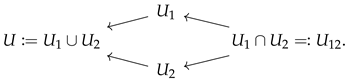
A presheaf is called a sheaf when this gluing condition holds. It can be formulated even for more general target categories, using the notion of an equalizer, but we do not do this explicitly here. An analogous gluing condition gives the condition for a presheaf on a more general site, such as , to be a sheaf. Sheaves on encode natural sets of locally defined data on some class of d-manifolds equipped with geometric structure.
- 2.2.4. Examples of sheaves. We quickly list just a few basic examples (and classes of examples) of the above constructions here.
- Given an object , the locally constant sheaf takes the value X on any connected open set. The gluing condition can be used to deduce its value on arbitrary open sets; when has direct sums, we find that , with .
- Suppose has a zero object. Then, given a space M and a point , the skyscraper sheaf takes the values
- Given a map of spaces and a sheaf on M, the pushforward is a sheaf on N, defined by takingfor every open set . There are other natural operations on sheaves associated to maps between spaces, which we do not discuss in detail here.
- For M a smooth manifold, the smooth sections of any vector bundle over M form a sheaf.
- The space of smooth maps from M into a target space X; to every open set U, we assign , with the obvious notion of restriction. (The fields of the nonlinear sigma model arise in this way.) In fact, this example defines a sheaf on the smooth étale site: To any smooth space, we assign its space of smooth maps into X.
- The solutions to any local partial differential equation define a sheaf.
- A map of vector bundles defines a map between the corresponding sheaves of sections. The kernel and cokernel of such a map are not necessarily vector bundles—but the kernel and cokernel of the map on sections do define sheaves.
- 2.2.5. An important non-example. This example is so important that we will give it special typographical emphasis:
Gauge equivalence classes of fields do not form a sheaf!
- One easy way of seeing this is the familar Aharonov–Bohm effect [17]. The electromagnetic field is a connection, and its vacuum configurations are described by the condition that its curvature vanishes. Locally, over any open set, any such flat connection is gauge-equivalent to the zero connection. But the space of gauge-equivalence classes of vacua on is of positive dimension, corresponding to the possible holonomies of the gauge field around the excluded region. The corresponding phase effect is observable [18].
Dogma 1.
Physical gauge field configurations are not described by the collection of gauge equivalence classes of gauge fields. They are described by the sheaf of gauge fields, together with the collection of equivalences on it described by the sheaf of gauge transformations.
The relevant mathematical structure for describing the physical configurations of the fields in a gauge theory is, thus, not a set (a collection of objects without any further structure), but rather a groupoid (a collection of objects together with a set of invertible equivalences between any pair of them). A careful treatment of related issues and gluing phenomena in the simple example of Dijkgraaf–Witten theory is given in [6], and we refer the reader there for further discussion and to build intuition.
This is the beginning of an answer to our question in §2.1.7: The idea of a space as a set (with some structure) is not flexible enough to accommodate physically important examples of the “space of fields”. We will need to extend it to include groupoids or, possibly, further higher structures.
- 2.2.6. Moduli spaces. To close this section, we remark briefly on the concept that we have arrived at in the previous example, which is often referred to as a moduli space. At an intuitive level, moduli spaces classify objects: There is one point for each object, and point A is close to point B when object B is, in some appropriate sense, a “small deformation” of object A. This general theme will be ubiquitous in what follows.
It is not really meaningful, though, to say that there is one point per object; we need to specify what we mean for two objects to be the same. (There is no “set of all possible vector spaces.”) As such, we need to identify a collection of objects, together with an appropriate notion of isomorphism or equivalence. A moduli space is, thus, associated to a groupoid of objects; we arrived at this idea above in the context of trying to understand the moduli space of inequivalent gauge field configurations.
Being isomorphic is, of course, an equivalence relation on the objects of a groupoid, so we might imagine building the set of inequivalent objects in a groupoid by dividing out by this equivalence relation. But then we run into a problem: Because an object can be equivalent to itself—and is so, in nontrivial fashion, precisely when it has symmetries—the elements of this set are not all alike!
As a simple example, one can consider the category of finite-dimensional real vector spaces, with equivalences being linear isomorphisms. Any object in this groupoid is equivalent to one of the objects , and this “gauge fixing” allows us to think of the equivalence classes as labeled by the nonnegative integers n. (The dimension is a complete invariant.) But the point represented by has the group of autoequivalences, and this group depends on n.
The reader who has seen the moduli space of elliptic curves before will find it pleasing to note that there are precisely two with additional symmetries—the ones corresponding to the square and the hexagonal lattice in —and that these correspond to the two orbifold singularities of the moduli space.
3. Resolutions
3.1. From Local to Global
We observe that we can evaluate a sheaf on a space in two ways, one of these being the obvious one. The other way is more complicated, but is motivated by ideas about using only local operations. The second way is better and, perhaps surprisingly, provides strictly more information.
- 3.1.1. Constraints. Thinking about the example of the locally constant sheaf makes it clear that sheaves can contain global information—even though they model locally defined data. Knowing the value of a locally constant function at any point in M determines everything there is to know, if M is connected. There are many examples of this: Knowing a holomorphic function in an open neighborhood of a point determines it in larger open neighborhoods by analytic continuation. Equations of motion in physics are typically well-defined boundary problems, so that knowing the value of a solution on uniquely determines that solution anywhere in U.
Each of these examples can be viewed as a subsheaf of the sheaf of smooth complex-valued functions on M, picked out by a certain local constraint. Locality means that the constraint is a differential operator: A function f is locally constant when , is holomorphic when , and satisfies the Laplace equation (or massless wave equation) when . Presenting things this way makes it clear that it is the constraint that allows the information contained in a local section to propagate to distant regions of M.
An important question presents itself at this juncture: How much global information about M is contained in, or can be measured by, the failure of a sheaf to behave fully locally? And how can we measure this information? To come up with an answer, we will engage in a bit of storytelling, motivated both by the physical idea of local observers in a global spacetime and by our ideas about gluing from above. Nothing in the story we will tell is precise or directly meaningful from either a physical or a mathematical perspective; we just want to give an intuitive picture of how physics-minded reasoning leads one naturally to the discovery of sheaf cohomology.
- 3.1.2. Gedankenexperimente. Imagine that a space X, for simplicity a d-dimensional smooth manifold, is populated by a collection of local observers. Each of them can observe only some neighborhood of their immediate location, which we assume must be contractible. (This assumption is intuitively reasonable if, for example, we imagine that these regions are defined by some inequality on the geodesic distance. More generally, since any point in a manifold has a neighborhood that locally looks like affine space, we can think of this as a “smallness” assumption on the observers: They should not directly observe any global topology.)
Suppose also that X is equipped with certain classical fields or local degrees of freedom, in the form of a sheaf . An observer located in the region can make measurements that pick out a local configuration of these fields—so a specific section in . How could we imagine piecing together information about a global section using only such local measurements?
Suppose that the neighborhoods and overlap, but the observer in is not contained in and vice versa. It is, thus, not possible to make a direct comparison. But if we wish, we can imagine placing a secondary observer—an “observer of observers”—in the overlap region . If this observer is also to be small, the overlap itself should again be contractible. We can ask that this observer report the mismatch between the value of a local section as reported in and as reported in . If this mismatch is zero, the gluing condition ensures that the local observers agree, and thus that we have a valid measurement on the union .
Of course, the procedure may not stop here. Conceivably, there could be triples of regions which share a threefold overlap. If this is the case, we also have three pairwise reports on the mismatch: one in , one in , and one in . In addition, there is a consistency condition on those mismatches that needs to be checked: Since the observer in , for example, is supposed to be reporting the difference between local measurements in i and j, it must be the case that . To verify the honesty of the observers of observers, we should place additional third-order observers—watchers of watchmen—on the triple overlaps , and so on.
- 3.1.3. What is the result of this procedure at the end of the day? Drawing a diagram of all of the reports of all of the watchmen, we see that we have a diagram of inclusion maps between elements of of the following form:
Summing this up, we can say that the diagram of spaces (12) has the property that, at every step, any two points that map to the same point on the left are the subject of a pasting rule, meaning they receive a pair of maps from a single point at right. For example, a point in and a point in map to the same point in precisely if they are the images of a common point in . Although it does not make sense to talk about an exact sequence in this context, the reader will no doubt see the analogy. If we remove X from the left of the sequence (12), we are left with a diagram of spaces, each of which is contractible (thus, from a topological perspective, “boring”). The arrows in this diagram give us a recipe for pasting together X from boring objects.
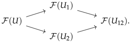
- 3.1.4. Applying the functor of sections of our sheaf to (12), we obtain a diagram in the target category:
The punch line, though, is that the sequence (13) need not be exact in the target category! We, thus, have two ways of placing the sheaf on the global spacetime X. Doing so naively just returns its global sections; doing so locally—using a system of local observers, observers of observers, and so on—produces a sequence of objects of , given by the cohomology groups of (13). The zeroth of these is , and the higher ones may or may not vanish.
Intuitively, one can imagine that the higher cohomology groups of order k represent potential failures of error correction at the level of the k-th-order watchmen. A nontrivial element of the k-th cohomology group is represented by a collection of reports on -fold overlaps, which are consistent in the sense that they agree on all -fold overlaps, but nevertheless cannot arise as the mutual errors of a set of incompatible reports on k-fold overlaps.
- 3.1.5. Names. We introduce some terminology after the fact. Omitting the first term, the diagram (13)—obtained by applying our sheaf to a diagram showing us how to populate X with local observers, or (equivalently) how to paste X together from contractible open sets—is called the Čech complex, and its cohomology is called the Čech cohomology of the sheaf. When X is a nice enough space, such as a manifold, this cohomology is the same as the sheaf cohomology of , and the higher cohomology groups are the derived functors of the functor of global sections.
Taking a step back, we observe that applying to a replacement of X—one that gave an explicit recipe for constructing it out of boring objects—gave more information than naively applying to X in the obvious way. As we will continue to see in what follows, this additional information is not there by accident; rather, it detects sophisticated global features of the space. So one is led to the philosophy that it is always better to think of subtle objects as pasted together out of simple ones. This is the first core observation of derived geometry.
3.2. Resolutions by Fine Sheaves
Instead of pasting together the space X from local neighborhoods, we come up with a recipe for pasting together the sheaf from “boring” ones. In the process, we rediscover de Rham cohomology.
- 3.2.1. Flabbiness. One obvious circumstance that ensures that the sequence (9) is exact is if the restriction map
The basic example of a flabby sheaf is the sheaf of all functions (in particular, with no requirements as to continuity). It is obvious here that local information tells us nothing at all about global behavior: The value of a function at a point bears no relation whatsoever to its values at any other point.
On the other hand, it is clear that flabbiness excludes many interesting examples. In particular, one has the intuition that continuous functions and smooth functions can be extended more or less at will, and that no constraints allow information to propagate over finite distances. Nevertheless, neither of these defines a flabby sheaf. This is because continuity requires that a function f, evaluated at the limit point x of a sequence of points , must be the limit of the . But for a partially defined function on an open subset U that contains all the but not the limit point, this limit may not exist due to convergence issues. (Consider the function on the positive real line.)
- 3.2.2. Fineness. The essential issue with continuity is that, given the value of a continuous function at a point, its value at infinitesimally close points (though not at any finite distance) is constrained. This suggests an obvious weakening of the condition of flabbiness: A sheaf on a manifold is called fine if, for any pair of sets , any local section over U, and any closed set , a section over V can be found that agrees with everywhere in K. (We are not being careful about what it means to restrict to a subset that is not open; this is not, strictly speaking, an operation that is a priori meaningful for an arbitrary sheaf. For functions or sections of vector bundles, the notion is intuitively clear; for the general case, we refer to [19,20].)
Fine sheaves are common: Sheaves of continuous or smooth functions (or sections of vector bundles) on a manifold are fine, and most of the interesting examples that appear in nature seem to be of this type. Indeed, in every example we will see later, we will actually work with locally free sheaves of -modules, or—what is the same—sheaves of sections of smooth vector bundles [21]. Most importantly for our purposes, fine sheaves have no higher cohomology ([20], Chapter II, Theorem 9.11). As such, the two prescriptions for going from local to global we identified above—the naive and the “derived” one—agree for fine sheaves, and there are no subtleties in working globally on spacetime.
- 3.2.3. Imposing constraints locally. Our prime example of a sheaf where local information obviously constrains faraway behavior was the locally constant sheaf . Interestingly, this sheaf is a subsheaf of a fine sheaf: There is an obvious inclusion map
The similarity to the first terms of (12) is disconcerting. Above, we covered a subtle space X by a family of boring spaces that map to it. By recording overlaps and continuing the sequence out to the right, we obtained a recipe for pasting together X from contractible local neighborhoods.
It is intuitively clear that one should try and continue (15) to the right, using the differential to explicitly encode the constraints that a locally constant function must satisfy, the relations between those constraints, and so on. If we are lucky, we will be able to do this using only fine sheaves, such as sheaves of smooth sections of vector bundles. This will result in a recipe for constructing by pasting it together out of sufficiently boring objects.
- 3.2.4. A smooth function is locally constant precisely when each of its derivatives vanishes at every point. Succinctly, f is locally constant when it is annihilated by the exterior derivative operator d. This tells us the first step of our resolution: We can take
From this point, the procedure is certainly well-known to the reader. The Poincaré lemma describes the next constraint, which is related to the fact that partial derivatives commute. The operator that appears is just the exterior derivative again. At the end of the day, our desired replacement for the sheaf on the site of smooth d-manifolds is just given by
To sum up, the de Rham complex is a replacement for the locally constant functions. It is a recipe for pasting together a constrained sheaf out of fine sheaves. As we will see in the next sections, many constructions in quantum field theories are about constructing replacements of precisely this kind. We underscore the importance of this pattern:
Dogma 2.
To understand a complicated object, identify a class of sufficiently boring objects, together with a technique for pasting together any complicated object out of boring ones. Then, understand the correct notion of equivalence between different recipes for pasting together the same object. Then, throw the original object away.
- 3.2.5. Local constraints replace local observers. We now have an easy way to see the fact that the Čech cohomology groups we associated to the sheaf on a space X above are nothing other than the de Rham cohomology groups of X. (This pattern of argument is extremely common, and goes back in this example to [22].)
We simply imagine placing the replacement for our sheaf—so the de Rham complex —on our replacement for X, which was the entire pasting diagram in (12). Since each sheaf involved is fine, there is no obstruction to pasting, so the result is equivalent to , and, thus, to the de Rham cohomology of X. But since each neighborhood in the pasting diagram is contractible, there is also no obstruction to appealing to the Poincaré lemma and replacing by on each of the U’s. Thus, the result is also equivalent to the Čech cohomology of on X.
3.3. Resolutions of Invariants
Having intuitively understood the idea of a functor failing to be exact in one example, we move on to another case of physical importance: the functor of invariants, with respect to the action of a group or Lie algebra. (This functor is one part, though not all, of the operation colloquially called “gauging”; see § 6.3.1.) In a certain schematic sense, the structures we will uncover were already present in (17).
- 3.3.1. Let be a Lie algebra. For simplicity, we work in the category of linear -representations over a field of characteristic zero (say or ).
There is a functor Inv from to Vect, defined by sending a -module A to its -invariant subspace
Since a -equivariant map carries invariant elements of A to invariant elements of B, it is clear how the functor is defined on morphisms.
- 3.3.2. The fundamental observation in the case of sheaves had to do with studying the basic pasting diagram (7)—an analogue, in spaces, of a short exact sequence. Applying the functor defined by the sheaf, we observed that the resulting sequence (9) was necessarily exact on the left, but not on the right. The failure of (9) to be exact was the origin of the higher cohomology of the sheaf.
We, thus, begin by studying a short exact sequence
of -modules, which we think of as representing a recipe for pasting the -module B together out of the constituents A and C. Applying the functor of invariants, we get maps of vector spaces of the form
Let us study what exactness of this sequence at each point translates to in detail.
Exactness at the left point means that invariant elements in A map injectively to invariant elements in B. This is clear, since the map from A to B was injective, so the sequence is exact on the left.
Exactness at the midpoint means that two invariant elements of B that represent the same equivalence class in C necessarily differ by an invariant element of A. This is also intuitively clear: By exactness of the original sequence, we know that lies in the image of A. But if b and are invariant vectors under , so is , which is, thus, in the image of .
The reader will have guessed that (20) will not be exact on the right, so it remains only to grasp intuitively why exactness should fail here. The essential point is that being invariant in the quotient space is a strictly weaker condition than arising from an invariant element in B. If we denote the quotient map by , then precisely when
But this just means that , which can occur without b being -invariant!
- 3.3.3. Derived invariants. By now, the path should be clear. Given a -module A, we should try and impose the condition of being -invariant explicitly, “at the cochain level”, rather than strictly. By doing this, we should arrive at a recipe for “pasting together” the subspace out of copies of A.
The beginning of the sequence is intuitively clear. The action of on A is given by a linear map
By duality, we think of this as a map ; the kernel of this map consists precisely of the invariant subspace . We, therefore, have the first steps in our pasting diagram,
Compare this with (16), placed on the flat space . There, we could have picked out the subspace of locally constant functions by asking that they be invariant under the action of the abelian Lie algebra of translations. Cartan’s magic formula says that the de Rham differential precisely agrees with this module structure when acting on functions.
This observation gives us a clue as to how the sequence should proceed. In that case, we had an antisymmetric relation, related to the fact that partial derivatives commute. For a more general Lie algebra, we will again have an antisymmetric relation, encoding the Lie bracket.
Concretely, consider concatenating the map with itself (or more precisely, with ). Doing this, we get a map from A to , which we can project onto the antisymmetric bilinear forms to get a map
This is the analogue of the commutator of partial derivatives; here, it should not vanish, but nevertheless should be redundant, as it is equal to . To get a square-zero differential, we can correct by letting the differential act on by the dual of the bracket map,
(We should assume that the dimension of is finite here, but will pass over this and related issues in silence.) The reader will check that, if we extend it as a derivation, defines a square-zero differential on
which has degree if we regard , analogously to the generators of the algebra of differential forms, as having degree . Written with respect to a basis of , the differential takes the form
This complex is called the Lie algebra cochains of with coefficients in A, and goes back to the work of Chevalley and Eilenberg [23]. While we did not, strictly speaking, show this, it is a good replacement for the naive functor of invariants, in the sense that its higher cohomology computes the derived functors.
- 3.3.4. It should also be apparent to the reader who has seen the BRST formalism for gauge theories [24,25] that we are recovering the basic ingredient of that formalism in a much more general setting. If we take the module A to be the smooth functions on some space, we can think of the Lie algebra cochains as being functions on a “graded manifold” . In cohomological degree zero, we recover -invariant functions, which are a model for the functions on the quotient space of X by the infinitesimal action of . In the context of the BRST formalism, the new degrees of freedom responsible for taking derived -invariants, which consist of the symmetry generators placed in degree , are the fields usually called “ghosts.”
- 3.3.5. A word on gradings. In the context of physics, every system is equipped with a grading by , called fermion parity or intrinsic parity. Physical degrees of freedom can be either bosons, represented by commuting fields, or fermions, represented by anticommuting fields.
As we are discovering, there is also a cohomological -grading to keep track of, which is sometimes called the “ghost number”. Our conventions are cohomological; every differential will have degree . Correspondingly, duals reverse gradings: If E is a cochain complex, then is such that . The cohomological shift functor is denoted with square brackets: . We adhere to the Koszul rule of signs for the totalization of cohomological grading and the internal parity, modulo two. Other conventions are possible. A lucid discussion of related issues is in ([26], Appendix to §1). Note, though, that our convention deviates from their “point of view I”, perhaps unwisely! Our choice is motivated by the desire to consider twists of theories in settings where the twist breaks the grading to an overall , as in [27]. We will use bosonic/fermionic to refer to intrinsic parity, and commuting/anticommuting to refer to overall parity.
A few illustrative examples: A physical fermion is a field of cohomological degree zero and odd intrinsic parity. A ghost field, representing a local gauge (bosonic) invariance, sits in degree and has even intrinsic parity, since it implements the action of a bosonic symmetry. The corresponding observable, often written with a notation like —which lives in the dual space!—is of degree and bosonic, thus overall anticommuting. The same applies to the symbols in the de Rham complex.
- 3.3.6. It turns out that thinking about Lie algebra cochains will allow us not just to construct a derived model for gauge invariants, but a derived model for an entire perturbative field theory. A version of this construction provides one possible answer to the open question from above (§2.1.7) about which notion of spaces we want to work with. We turn to this now, beginning with a bit of a detour through intuitive basic algebraic geometry.
4. Local Lie Algebras and Formal Moduli Problems
One good complementary reference for the material in this section is [28].
4.1. Intuitions from Algebraic Geometry
We discuss the relationship between a space and the algebra of of functions on it, working towards a basic feel for the correspondence between algebraic and geometric structures and an intuition for the idea of studying a space via the maps it receives from other spaces.
- 4.1.1. A basic observation. We start at the very beginning:
Observation 1.
There is a natural contravariant functor from spaces to commutative algebras over a field k, which sends a space X to an algebra of appropriate k-valued functions on X.
Here, “appropriate” is a placeholder for some set of conditions: continuity, smoothness, or whatever else. The action on morphisms is given by pulling back a function along a map of spaces. We are being intentionally vague about what kinds of spaces we are interested in; the reader is free to think of smooth manifolds and smooth functions, or of algebraic varieties and polynomial functions.
In the context of classical mechanics, we can think of this functor as going from state spaces to algebras of observables. (In a field theory, we could imagine X as the space of field configurations; classical observables, again, are functions on this.) In this context, we know that measuring observables should determine the state space in some fashion; this is, in fact, all we are able to do. So, one might naturally expect this functor to be an equivalence. Taking this intuition seriously is the starting point of algebraic geometry.
- 4.1.2. Measurements. Imagine that we are interested in a physical system with algebra of observables A. To perform a simple measurement, we select an element , and inform an experimentalist that we are interested in knowing what value f takes. After taking appropriate action in the world, the experimentalist returns some numerical value a. (Better yet, we could engage with the world of phenomena ourselves. For the sake of brevity, though, let me refrain from turning down that road.)
This measurement tells us that the equation holds in our system. But it tells us a bit more than this: Since there is an algebra structure on observables, we also know (for example) that , and that for any other observable g. The algebraic structure we are discovering is that of an ideal in A: This ideal is generated by the single element , and it consists of all elements of the form . If f has been measured to be a, we know that all observables in this ideal must vanish.
Ideals are subspaces with the property that
One should think of an ideal as being the kernel of a map of commutative algebras. Indeed, if is such a map, then
so that is an ideal. Conversely, if I is an ideal, then we can equip the quotient of vector spaces with a natural commutative algebra structure by defining
The ideal property ensures that , so that the quotient map from A to is compatible with the product.
We can, of course, imagine more complicated sets of measurements than the one generated by . We might measure several different observables, for example. But the intuitive idea is clear: A measurement should give information about the system by specifying some subset of observables which one knows to vanish. By using the structure on observables, one sees that this subset should be an ideal. And it would be reasonable to try and take this as a definition:
Idea 1.
Given a commutative algebra of observables A, a measurement is an ideal.
In exploring whether or not this idea makes sense, one is led to a number of interesting phenomena. Traditionally, in algebraic geometry, one tried to hew to one’s traditional notion of space by imposing restrictions on the sorts of algebras A and ideals I that one was interested in. Modern perspectives tend to reverse this logic, using algebraic phenomena to lead one to broader and more abstract intuitive pictures of geometry.
- 4.1.3. Numerical measurements. (The author owes many of the following explanations to discussions with Minhyong Kim, whom he acknowledges with gratitude.) One important class of ideals correspond, intuitively, to “measurements valued in numbers.” Since there are no obstructions to simultaneous measurement in classical mechanics, such measurements should specify a numerical value for all observables. We expect that numerical measurements “determine the state”, so we would like to arrive at a notion that captures the idea of a “point” in the state space.
To specify “numerical values” for all observables should be to give a map
where k is some field of numbers. (At this level of abstraction, we do not specify k more narrowly.) To each observable, this map assigns its numerical value. Being a map of algebras ensures that these measurements are coherent: The value of is the product of the values of f and g. On general grounds, p will factor into a quotient followed by an inclusion:
where is the ideal corresponding to the measurement in the sense of Idea 1.
So, maps injectively into a field. This does not mean that is itself a field—but it does mean that cannot have zerodivisors. Such a ring is called an “integral domain”. A quotient ring is an integral domain precisely when the ideal I is prime: This means that the product of two elements f and g lies in I only when at least one of f or g also lies in I. (To understand the name, one should recall that a prime number p divides a product only when p divides either m or n.)
We are, thus, led to the the idea that numerical measurements of an algebra of observables A correspond to prime ideals in A. And, in fact, this is exactly how the correspondence between spaces and rings in algebraic geometry works: The spectrum of a ring, , is defined as its set of prime ideals. Additionally, the spectrum is a functor: A map of rings determines a map , by taking preimages of prime ideals. (The spectrum is the inverse operation of the functor from Observation 1.)
- 4.1.4. The generic point. There is an important distinction to make at this juncture, which is most easily seen by considering the simple example of polynomials in one variable, . We think of these as polynomial functions on . What are the prime ideals here?
A nontrivial ideal is generated by a collection of polynomials . In fact, for any non-empty such collection, we can find a unique polynomial f that generates the same ideal: the greatest common divisor of the . The ideal generated by f is prime precisely when f is irreducible, and the irreducible polynomials in one variable over are just the linear ones: , for . So, things look pretty good for a correspondence between prime ideals and “points” in in the normal sense.
Each of the ideals we have defined so far is, in fact, maximal: It is not contained in any other proper ideal. Maximal ideals I are precisely those for which is itself a field: In our example,
If we think about an algebra of functions on a space, restriction to a point should have this property: The algebra of functions on a point is just the field in which the functions are valued.
But is itself an integral domain! Correspondingly, the ideal 0 is a numerical measurement—albeit a “null measurement”, in which we do not specify the value of x at all. One related map into a field sends to , the field of all rational functions on .
- 4.1.5. Maximal measurements. Having understood this, we have arrived at the correct intuition. A point in consists of a possible numerical measurement, which may or may not be maximal. (It may provide incomplete numerical information.) If A comes to us as the algebra of functions on some space X, we can imagine each point as some subspace (of whatever dimension) of X that can be cut out by numerical measurements. In particular, the entire space X (the “generic point”) is a point of .
A subset of the points consists of maximal ideals in A (the “closed points”). Maximal ideals correspond to maximal measurements, and the set of all maximal ideals is called the maximal spectrum of the algebra A.
In fact, is naturally a topological space. (So is ; we are in fact describing the topology there, restricted to the closed points.) The topology has a canonical basis, labeled by observables : The corresponding set is
In words, is “the set of states in which the observable f does not vanish”. Since an observable being nonzero is an open condition, it makes sense to think of as an open set in the state space. This topology is called the Zariski topology; it is most commonly used in the algebraic context, but it makes sense for any algebra or ring.
We can, therefore, reconstruct the state space from the algebra of observables, as we expected on physical grounds that we would be able to do. A version of this intuition is captured in the following proposition.
Proposition 1
([29], Chapter 1, Exercise 26). Let X be a compact Hausdorff space, and let be the commutative algebra of continuous real-valued functions on it. Then, is homeomorphic to X.
The moral of the story is that the topology of the space of states can be observed.
- 4.1.6. Unreliable experimentalists. Returning to Idea 1, it is natural to ask about the physical relevance or intuitive meaning of the other ideals that we have been ignoring. Again, we will just think about the basic example .
As we have said, any nontrivial ideal is generated by a single polynomial f, which we can factor as a product of linear polynomials:
with the distinct roots of f. So, there are two somewhat distinct-feeling phenomena to digest: a measurement corresponding to several closed points, and a measurement corresponding to a single closed point with some multiplicity.
The former makes instinctive sense. It is natural to imagine a measurement that gives partial information about a system in the form “ or ”. While this measurement is not numerical—“0 or 5” is not a number—it is nevertheless meaningful.
The latter case is a little more subtle. For concreteness, we consider the polynomial . In our interpretation of an ideal—the observables we know, with certainty, to vanish—this is saying that , but without being able to conclude that .
Thinking about the sorts of approximate computations one learns to perform in undergraduate physics, working order by order in a small parameter and treating terms of order as negligible, we can imagine that the experimentalist is reporting that x is of order —thus, in a formal sense, infinitesimal. This is, again, not really a numerical measurement, but is nevertheless part of a class of statements that we are operationally accustomed to working with. We emphasize that it already points to the idea of a family of measurements: To say that x is of order is, in principle, to make reference to a tunable parameter whose value is taken to be small. The intuitive connection between nilpotent ideals and perturbation theory goes much deeper, and we develop it a bit more in the next sections.
4.2. The Functor of Points
We review, at a completely schematic level, the basic idea of the functor of points, and discuss, in vague terms, some physically relevant generalizations of the notion of “space” that it suggests.
- 4.2.1. The definition. Having absorbed our notion of “point” from above, there are a few powerful generalizations of the basic idea that we can consider. The essential idea, already sketched above, is that we can imagine measurements of different types, according to where the “evaluation map” is valued. For instance, we can think of as being the set of real points of A, as being the set of complex points, and so on. (If A is an algebra over R, such maps will automatically be surjective and, thus, define maximal ideals.) Since a field k has no nontrivial ideals, consists of only one point, and maps from A to k can be thought of dually as maps of spaces of the form
For more general prime ideals, such as the ideal generated by in , the quotient is not a field: It is isomorphic to polynomials in one variable, , with the map sending both x and y to z. But we still get a map on spectra,
which sends the closed point to the closed point . We can imagine the space of ring maps, , as parameterizing the collection of all maps of spaces from to , or “all subspaces of of shape ”, or “all families of points in parameterized by z.”
This suggests the following definition: Given a commutative ring S, the functor
is called the functor of S-points. (It might be more intuitive to remember “functor of S-families of points.” The erosion of the distinction between point and subspace already started above, when we observed that Spec is better-behaved than Max.) Dually, if we imagine some category of spaces and a test object Z in that category, the functor of Z-points will be . (In the example, think of .)
- 4.2.2. Abstracting away from this, it is useful to think about such a functor of points as being a generalization of a space of the form . Certainly, any space that is at least locally modeled by some defines a functor of points. But not any functor deserves to be called a functor of points: Thinking of the example of the sigma model in §2.2.4, it is clear that we should ask for some sort of gluing condition on the set of test spaces, giving us a notion of compatibility between the space of Z-points and the spaces of -points when the test spaces form a “covering” of Z in an appropriate sense. Interesting generalizations of the notion of space arise when a functor has all of the properties of a functor of points—in particular, satisfies locality, in the form of a “gluing” or “descent” condition—but is not represented by any space.
Thinking further along these lines, one naturally comes to the idea of a moduli functor: To a space, we can associate (for example) the collection of principal G-bundles on it, or the collection of principal G-bundles with connection, or some other space of fields. Such an object is obviously natural in the context of quantum field theory, and it also clearly wants to be thought of as a functor of points—even when it does not arise as a space of maps into a fixed object. (The reader may instinctively think about classifying spaces here, and is welcomed to do so.) However, recalling Dogma 1 from §2.2.5 above, it should be clear that moduli functors cannot, in general, be valued in the category of sets! Rather, they are usually a functor from test spaces to groupoids, satisfying a gluing condition that makes them into a sheaf in an appropriate sense.
What we are grasping at here is the idea of a stack. We will not be able to go too deeply into related issues, but refer to [30] for a careful and readable intuitive overview, and to the vast literature on the subject for the actual details ([31], for example).
- 4.2.3. At this point, one might now attempt to describe the “space” of fields in a field theory on a manifold M using a sheaf of groupoids on some category of test spaces. To a test space Z, we assign the groupoid of families of gauge field configurations on M parameterized by Z.
To get to the formalization we will actually discuss in the remainder of this article, two more small steps are necessary. The first of these is less dramatic: It just involves remembering that gauge invariances are not the end of the story. To get to a description of a p-form gauge field, for example, one first parameterizes the gauge equivalences by the space of -forms, where a -form c sends to .
These gauge transformations, however, have redundancies: If two gauge parameters induce the same gauge equivalence transformation on , they can, and should, be viewed as themselves equivalent. And, following Dogma 1, we should remember the equivalences between equivalences, rather than dividing out by them. So, we add “ghosts for ghosts”, parameterizing equivalences between gauge parameters, and so on. We will pass over all of the resulting technicalities in silence, but it is important to mention that simplicial sets, rather than just groupoids, appear as a target category for precisely this reason (for example in [7], to which we refer for further discussion of this point). We will have a bit more to say about simplicial sets in what follows, but for now, it is a sufficient intuition to think of them as a “higher” version of groupoids, where objects are thought of as 0-simplices, equivalences as 1-simplices that join them, equivalences between equivalences as 2-simplices, and so on.
- 4.2.4. The second step involves pinning down the relevant category of test objects, which ends up being the following:
Definition 2
([1], Appendix A.2). A dg local Artin algebra is a finite-dimensional, nonpositively graded differential commutative algebra A over with a unique maximal ideal , closed under d and satisfying .
We comment briefly on each aspect of this definition. “Artin” here corresponds to the condition of finite-dimensionality on A, and means, very roughly, that we can think of the space as being zero-dimensional. “Local” refers to a ring that has a unique maximal ideal, which—as we recall from above—corresponds to a space that has only one point. Finally, we allow for differential graded algebras as probe objects because we are also interested in understanding the derived structure of the space we are probing.
That this is necessary is illustrated by familiar phenomena in supergeometry: A normal manifold is determined by its points over a field, as we saw above, so fields are a sufficient class of test objects. But the ring of functions of a supermanifold has no points other than those that come from the underlying bosonic manifold. To probe its structure, we must extend our class of test objects to include “superpoints” with arbitrary numbers of auxiliary Grassmann variables.
A basic example of a local Artin algebra to keep in mind is , with x (for example) in degree zero. The unique maximal ideal is generated by x. Let us imagine, for simplicity, that we are probing a space X that is cut out by some equation f in a larger affine space . An A-point of X then corresponds to a chosen point p in X (the image of the unique point of A), together with a one-parameter family of points in that lies within the zero locus of p up to terms of order . Using test spaces of this form, we are, thus, able to probe nearby solutions at any finite order in perturbation theory.
- 4.2.5. Formal moduli problems. At this point, the reader should hopefully be able to guess the outline of the definition of a formal moduli problem, which we quote here for the sake of completeness. Let denote the category of dg local Artin algebras, as defined above, and the category of simplicial sets ([7], Definition 4.9).
Definition 3
([32], Definition 0.0.8). A formal moduli problem is a functor
for which is contractible, and for which every pullback diagram
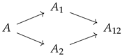 gives rise to a homotopy equivalence between and .
The technical details of this definition are irrelevant for our purposes here, but we will again try and build intuition for the requirements in terms of things we have seen before. The reader will hopefully recognize the second property as being an instance of a gluing condition: The pullback diagram (40) is yet another example of (7), the arrows appearing backward because Spec is contravariant.
The first condition just abstracts the idea that the functor should behave like the formal neighborhood of a point in a space. It says that the functor should associate just a point (a contractible simplicial set) to the field , which just consists of a point with no additional infinitesimal information. In this sense, it is a normalization condition.
4.3. Deformation Functors
We discuss the duality between dg Lie algebras and formal moduli problems and, finally, define a local Lie algebra.
- 4.3.1. We now want to lay the final stone in the winding path of intuitions that is bringing us to the notion of a local Lie algebra. The essential idea involved is both old and deep. I quote it here in Lurie’s formulation:
Dogma 3
([32], page 2). If X is a moduli space over a field k of characteristic zero, then a formal neighborhood of any point is controlled by a differential graded Lie algebra.
Pieces of this idea go back, at least, to Quillen’s work on rational homotopy theory [33] and Sullivan’s theory of minimal models [34], and there are important antecedents even before that in Kodaira and Spencer’s theory of deformations of complex structure [35] and in the work of Nijenhuis and Richardson [36]. The general philosophy articulated above seems to have congealed in the Zeitgeist in the late 1980s, appearing clearly in a 1987 letter from Deligne to Millson [37] and a 1988 letter from Drinfeld to Schechtman [38]. Extremely general versions of this statement that are nevertheless concrete enough to be amenable to proof were formulated (and then proved) by Pridham [39] and also by Lurie [32], building on important earlier results (in a somewhat narrower context) by Hinich [40] and Getzler [41]. I cannot hope to sketch the polycentric history of this idea fully here; the reader is referred to [42] for a recent review.
The rule is a simple one ([41], Proposition 1.1): Given a dg Lie algebra (or, more generally, an algebra) , its Lie algebra cochains (§3.3.3) are a commutative differential graded algebra . The moduli space we want to consider is, morally speaking, the spectrum (§4.1.5) of this cdga.
The spectrum of a cdga is not a space in a usual sense, but it can be understood as a simplicial set ([34], §8), which the reader should think of as a higher version of a groupoid (§4.2.3). Since we have anticipated the necessity of thinking of our spaces of fields as simplicial sets, this should be unsurprising.
To define the k-simplices of this simplicial set, we let denote the space of (polynomial) de Rham forms on the standard k-simplex. Then, the k-simplices of are defined by homomorphisms of commutative differential graded algebras from to . Getzler shows that this simplicial set can be thought of as the space of solutions to the Maurer–Cartan equation
where denotes an element of the dg Lie algebra .
We can define the formal moduli problem associated to by specifying its functor of points as follows: Let A be an object of with maximal ideal . The zero-simplices of the simplicial set are solutions of the Maurer–Cartan equation in . More generally, the set of k-simplices is defined to be the set of solutions of the Maurer–Cartan equation in .
- 4.3.2. Applying this general philosophy in the context of field theory, Costello and Gwilliam give a definition of a local Lie algebra which is adapted to describe any natural formal moduli problem defined by local partial differential equations on a manifold.
Definition 4
([1], Definition 3.1.3.1). A local Lie algebra on a smooth manifold X is a graded vector bundle on X, equipped with polydifferential operators
that make its sheaf of sections into a sheaf of algebras on X.
We remark that the condition that arises as the smooth sections of a graded vector bundle is in place to ensure that is a fine sheaf. Thus, all issues relating to placing on an interesting global geometry have already been resolved. The reason that algebras appear instead of (dg) Lie algebras is just that we are working in the context of cochain complexes up to homotopy, where one cannot, in general, ask for algebraic conditions (such as the Jacobi identity) to be strictly satisfied. We regret that providing more complete intuition for this idea would take us too far afield at the moment; instead, we refer to the excellent treatment in [43].
The notion of a local Lie algebra on a site of structured manifolds is immediate; as a simple example on the site of smooth manifolds, one can consider the tangent bundle in degree zero. Numerous less trivial examples follow in the next section.
The following point should, by now, have been driven home:
Dogma 4
(Developed at length in [1,5]). If is any sheaf of spaces (or derived stacks) on some site of structured manifolds, the formal neighborhood of a fixed section f is described by a local Lie algebra on .
Recall that the space described by a local Lie algebra is the space of its Maurer–Cartan elements, or equivalently, the spectrum of its Lie algebra cochains. Since there is a shift by one in the definition of Lie algebra cochains, there is a shift between the grading on the Lie algebra and the conventions for cohomological degree in the physics literature, where observables are functions on the space of fields (without a shift), and where physical fields are placed in degree zero. Thus, a field theory described by a local Lie algebra has space of fields .
4.4. Variational Formal Moduli Problems
We make brief mention of shifted symplectic geometry and its role in the BV formalism. Regrettably, space does not permit us to go into more detail.
- 4.4.1. We have now completed motivating the definition of a local Lie algebra, and built up intuition as to why the definition is correct, why it is powerful, and what it can be applied to. It remains to understand which formal moduli problems correspond to perturbative Lagrangian field theories. In physics, the development of a derived approach to Lagrangian field theories was pioneered in groundbreaking work by Batalin and Vilkovisky [44,45,46], and still goes by the name of the Batalin–Vilkovisky formalism. We deeply regret not being able to discuss it at greater length here.
We will content ourselves with giving one key intuition, which is related to the calculus of variations. In a general set of natural partial differential equations, there is no connection between the degrees of freedom (typically some smooth functions or smooth sections of vector bundles) and the equations they are asked to satisfy. The system may be underdetermined or overdetermined.
Precisely when the equations of motion are variational, there is a sense in which equations of motion and degrees of freedom correspond. More precisely, they are in duality: Each field corresponds to its equation of motion
In light of Dogma 2, it is clear that we should model the space of solutions to the equations of motion by adding fields in degree that impose them. As it turns out, the pairing between fields and equations of motion can be interpreted as a -shifted symplectic structure in codimension zero. By an application of descent, this corresponds to the normal (0-shifted) symplectic structure on the phase space of a Lagrangian field theory, which is defined in codimension one. Noether’s second theorem, which establishes a pairing between gauge invariances and relations between equations of motion, ensures that this structure extends to gauge theories.
Dogma 5
([2] and many others: Pridham, Safronov, …). Locally variational formal moduli problems are precisely -shifted symplectic formal moduli problems.
Working in this framework, it is possible to consider degenerate examples of -shifted symplectic structures. This gives an approach to understanding at least certain classes of non-Lagrangian field theories, examples of which we will see below. Just as in the unshifted case, degeneracies can arise in one of two ways, which are in some sense dual: either to a -shifted presymplectic structure, corresponding to a constrained system or to a subspace of a nondegenerate phase space, or to a -shifted Poisson structure, corresponding to a subalgebra of the algebra of observables (such as a current algebra). Both are physically relevant, and we will return to this a bit more in what follows.
5. Examples
In this section, I will catalogue some useful examples of formal moduli problems—both field theories and symmetries—that appear in the literature.
5.1. Introductory Remarks
We alert the reader to a few things to watch out for in the sequel, as well as explicating some notation.
- 5.1.1. In what follows, I will try to use names for local Lie algebras that remind the reader of the formal moduli problems they represent. Mimicking the typical notation for Lie groups and Lie algebras, I will denote formal moduli problems with lowercase letters: for example, “” for infinitesimal deformations of a fixed flat G-connection. The corresponding full moduli problem, consisting of the space of all flat G-connections, would be denoted . We emphasize again that a formal moduli problem involves a choice of basepoint, analogous to the choice of vacuum in perturbative quantum field theory; our notation often does not indicate this choice explicitly, but it is always present.
- 5.1.2. Anomalies. The cohomological approach to anomalies, which identifies them as elements in a particular BRST cohomology group associated to the local Lie algebra representing the symmetry, has a long history. Implicitly, it goes back as far as the celebrated Wess–Zumino consistency conditions [47]; the subject was developed rapidly by the Italian school in the 1908s ([48], among others), and is by now very much a part of the standard lore. We cannot hope to review it here, and refer the reader to any of the comprehensive treatments in the literature [49,50,51].
For a local Lie algebra, the cohomology group classifying its potential anomalies is : Speaking roughly, these are cohomology classes represented by functionals on of degree that are spacetime d-forms, considered modulo the image of the spacetime de Rham operator. We will note a few of these classes in the examples in this section as we go along, and will meet anomalies again in the context of the factorization Noether theorem below.
- 5.1.3. Sphere algebras. It is worth emphasizing again that local Lie algebras are, in particular, sheaves of Lie algebras on an entire class of manifolds. They, therefore, contain much more information than a single symmetry algebra, and should not be confused with the values they take on flat space, or on any particular geometry.
One is often interested in the algebra of symmetry transformations that acts, for example, on point operators in a quantum field theory, or on the Hilbert space when quantizing on some -manifold Y. To get the corresponding algebras, we place the local Lie algebra on the complement of a point in , or on a cylinder of the form , respectively. In nice enough circumstances, one can relate the former to the latter by taking .
5.2. Locally Constant Symmetries
We discuss three different formal moduli problems whose zeroth cohomology is related to locally constant symmetry transformations valued in a Lie algebra .
- 5.2.1. Let be a finite-dimensional real or complex Lie algebra, and G a Lie group with . Let denote the site of smooth d-manifolds equipped with principal G-bundles P carrying a chosen connection. The connection induces a derivation ∇ of degree in the complex of de Rham forms valued in any vector bundle associated to P, in particular, in the adjoint bundle , which is a bundle of Lie algebras. The curvature is the tensor ; when the connection is flat, ∇ is a square-zero differential.
Formal Moduli Problem 1.
We work on the site of d-manifolds equipped with principal G-bundles with flat connection. The formal moduli problem of nearby flat G-connections consists of smooth differential forms valued in , viewed as a local dg Lie algebra via the Lie bracket inherited from and the differential given by ∇.
Placed on a manifold M equipped with a trivial principal G-bundle with trivial flat connection, reduces to the (local) dg Lie algebra .
In general, FMP 1 is not -shifted symplectic, and, thus, not variational. An exception occurs on three-manifolds: In precisely this dimension, is -shifted symplectic, and, thus, its perturbative version becomes a BV theory, known as perturbative Chern–Simons theory.
- 5.2.2. We now work again over the site .
Formal Moduli Problem 2.
The formal moduli problem of nearby G-connections on is given by the local dg Lie algebra
Working near the trivial connection in the trivial principal G-bundle, reduces to the two-term local dg Lie algebra
which is a quotient of the local dg Lie algebra in obvious fashion. Since it has no support above degree one, it is clear that FMP 2 is never variational. The Maurer–Cartan equation is trivial; the only interesting structure of the space of connections comes from the action of gauge equivalences on it.
Take to be abelian for simplicity of exposition. In even spacetime dimensions , there is a well-known anomaly cocycle on this local dg Lie algebra, corresponding to the chiral anomaly of Adler, Bell, and Jackiw [52,53]. To the best of our knowledge, the cocycle in BRST cohomology was first understood in [48]. The cocycle takes the form
- 5.2.3. Our third formal moduli problem is, in a sense, intermediate between and . For the sake of brevity, we describe it only near the trivial connection in the trivial principle G-bundle on M.
Formal Moduli Problem 3.
The formal moduli problem of perturbative Yang–Mills connections near the trivial connection on M is described by the local algebra
The structure contains 2-ary and 3-ary brackets, corresponding (via the BV formalism) to the cubic and quartic terms in the BV action, respectively. We will not need them further here and, so, omit an explicit description.
When admits a nondegenerate invariant bilinear form, for example, when is reductive, is a -shifted symplectic formal moduli problem.
5.3. Higher-Form Symmetries
In the abelian case, there are obvious generalizations of the previous formal moduli problems to connections in higher abelian gerbes (higher-form gauge fields). We sketch some basics quickly here.
- 5.3.1. Connections in higher abelian gerbes. We give some relatively obvious generalizations of the abelian versions of the above formal moduli problems to the setting of higher-form symmetry.
Formal Moduli Problem 4.
Let M be a smooth d-manifold. The formal moduli problem of perturbative connections in the trivial -gerbe, denoted , is described by the abelian local Lie algebra
A deformation of the connection is given by an -form. We note that there is a model for a non-perturbative version given by smooth Deligne cohomology. This is the cochain complex of abelian groups , defined on a smooth d-manifold to be
is a model for the entire nonperturbative stack of higher gerbes with connection. Regrettably, we cannot go into this in any detail here, but refer the interested reader to [54], or to ([55], §7) for a related discussion in the physical context of self-dual fields.
Formal Moduli Problem 5.
Let M be a smooth d-manifold. The formal moduli problem of perturbative flat connections in the trivial -gerbe, denoted , is
A deformation of the trivial flat connection is given by an -form, subject to the constraint that its -form curvature vanish. This formal moduli problem is shifted symplectic precisely when is even and . We recover the “higher abelian Chern–Simons theories”, generalizing normal Chern–Simons theory in the case . Again, smooth Deligne cohomology can be used to construct a model of the full nonperturbative moduli problem by adding a copy of the constant sheaf in degree .
Formal Moduli Problem 6.
Perturbative higher abelian Yang–Mills theory with gauge algebra is described by the abelian local Lie algebra
This formal moduli problem is shifted symplectic. An “electric” nonperturbative version is, again, obtained by adding a copy of in degree .
In order to describe the theory in a manner that can be locally coupled to both electric and magnetic charges, it is necessary to centrally extend it so that the cohomology contains the global symmetry that defines the magnetic charge. One can imagine this as working with the magnetic gauge potential as a fundamental degree of freedom. One models the resulting nonperturbative moduli problem by the complex
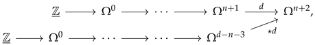 which one can think of as a pair of an electric (higher) -gerbe with connection -form A and a magnetic (higher) -gerbe with connection -form B, subject to the single mutual constraint that witnesses them as mutually dual.
As is shown in [55], the moduli problem (52) is -shifted presymplectic, and, thus, admits the structure of a (presymplectic) degenerate BV theory. For other work on (Poisson) degenerate field theories, we refer to [56].
Formal Moduli Problem 7.
Consider the étale site of -dimensional conformal manifolds. The formal moduli problem of perturbative self-dual higher gauge fields is controlled by the abelian local Lie algebra
Again, as was observed in [55], Deligne cohomology makes a nonperturbative definition of the moduli problem of self-dual higher -connections possible. It takes the simple form
This moduli problem is -shifted presymplectic, and dimensionally reduces to a complex of the form (52) in spacetime dimension [55].
5.4. Spacetime Symmetries
We study a few examples of local Lie algebras controlling deformations of geometric structures on spacetime.
- 5.4.1. Riemannian structures. The local dg Lie algebra met controlling deformations of (equivalence classes of) Riemannian metrics is defined on any smooth manifold M with Riemannian metric g. It takes the formWe denote fields in degree zero by and in degree one by h. The differential sends to , so that the cohomology in degree zero consists precisely of Killing vector fields. The brackets are such that vector fields act everywhere by Lie derivative.
- 5.4.2. Riemannian structures on the line. We write a degenerate example of this formal moduli problem (parallel to §2.1.8) explicitly in coordinates: the one-dimensional case. Working with respect to a generic coordinate s on the generic line, a metric is given by , where f is a globally nonvanishing function and denotes the tensor square (automatically symmetric in dimension one). As discussed above, we can choose an adapted coordinate t such that . A vector field is given by an expression of the form , with x again a function, and a perturbation of the metric by a tensor . The differential sends to the element ; the nonvanishing Lie brackets are
- 5.4.3. Conformal structures. Working on the same site, smooth manifolds equipped with Riemannian metrics, we can define a local dg Lie algebra conf controlling deformations of conformal equivalence classes of metrics. It takes the formWe denote fields in degree zero by , and in degree one by h. The brackets are such that vector fields act everywhere by Lie derivative and is the element of type h.
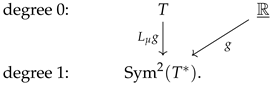
On even-dimensional manifolds, there are well-known classes in that are responsible for conformal anomalies. The classes are divided into two classes: The first, the a anomaly, takes the form
whereas the c anomalies (whose number depends on the dimension) are constructed as the product of with a strictly conformally invariant top form, built from copies of the Weyl tensor evaluated on the perturbed metric . These classes date back to [57,58]; a field theory classification was performed by Deser and Schwimmer in [59], and the fullly explicit classification of local cocycles for conf was completed by Boulanger [60].
- 5.4.4. Frames and G-structures. There is a model for the formal moduli problem of G-frames on d-manifolds, where G is a Lie group equipped with a map to . In the case where we choose or , the resulting moduli problem is equivalent to the moduli problem of metrics or of conformal structures, respectively. We refer to [9] for details.
- 5.4.5. Supersymmetries. We make the discussion of superconformal structures, briefly mentioned in §2.1.9, a bit more precise. Such a structure consists of a subbundle D of the tangent bundle of a smooth supermanifold M, of maximal odd dimension, such that the symbol, defined on the associated graded bundle by taking the image of the Lie bracket of vector fields in D under the projection to , is a locally trivial bundle of super Lie algebras. The typical fiber of this bundle, which is a two-step nilpotent super Lie algebra of the same dimension as M, is called the type of the superconformal structure. In physical terms, is the supertranslation algebra, and D specifies the vector fields on superspace that allow one to think of it as locally modeled by the flat superspace .
The formal moduli problem of deformations of superconformal structures is constructed for general in [9]; in physical examples, it reproduces the structure of the gauge algebra of the “Weyl multiplet” of conformal supergravity. We will study the example of superconformal structures in four dimensions in greater detail below.
5.5. Holomorphic Symmetries
We define a few natural formal moduli problems that appear in the study of symmetries of holomorphic theories. These are defined in general dimension, but are best known in complex dimension one, where evaluating them on the punctured complex plane returns the well-known Virasoro and Kac–Moody algebras.
- 5.5.1. The local (higher) Kac–Moody algebra. The constructions we explore here go back to [61,62] and were related to twists of current multiplets in supersymmetric theories in [63]. We work on a complex manifold X. Recall that a holomorphic vector bundle on X consists of a smooth vector bundle E over , equipped with a Dolbeault operator
- Leibniz: For any section of E and any smooth function f, we have(Note the abuse of notation: denotes both the holomorphic structure in the trivial bundle, arising from the complex structure on X, as well as the Dolbeault operator in E.)
- Cauchy–Riemann: After extending to as a derivation, .
Observe that is a partial flat connection in E, defined only for sections of the antiholomorphic tangent bundle . The first condition says that is a connection, and the second says that it is flat.
Let be a complex Lie algebra. We will say that a holomorphic vector bundle L is a holomorphic -bundle if its space of smooth sections is equipped with a Lie bracket, bilinear over smooth functions, that locally identifies L with the trivial bundle of Lie algebras with fiber , and if is a derivation of the Lie bracket. Basic examples are the holomorphic -bundle , where E is a holomorphic vector bundle of rank k, and the trivial bundle .
Formal Moduli Problem 8.
We work over the site of complex n-manifolds equipped with holomorphic -bundles L. The local dg Lie algebra controlling deformations of holomorphic -bundles is given by the Dolbeault resolution
with the Lie bracket obtained from the one on L.
Working near the trivial holomorphic -bundle, a description of the space of anomalies for this local Lie algebra was obtained in ([61], Proposition 1.25): the space of natural cocycles in is isomorphic to the space of degree- invariant polynomials. Here “natural” refers to the underlying complex manifold; on flat space, this means that a cocycle is invariant with respect to translations and rotations. The anomaly corresponding to an invariant polynomial is given by the local functional
where denotes a total section of . One can, of course, imagine transgression from the degree- “anomaly polynomial”, which would just be the corresponding component of evaluated on the curvature . Note, though, that is a total -form.
Specializing to , we observe that anomalies are parameterized by invariant bilinear forms on . There is, thus, a unique anomaly class for any simple Lie algebra , given by the Killing form. The anomaly takes the form
Placing this local Lie algebra on , we recover the Kac–Moody algebra associated to .
- 5.5.2. The local (higher) Virasoro algebra. We work on the site of complex n-manifolds.
Formal Moduli Problem 9.
The formal moduli problem of deformations of complex structure is controlled by the local dg Lie algebra resolving the sheaf of holomorphic vector fields:
The differential is the operator, and the Lie bracket is inherited from the Lie bracket of smooth sections of .
This is perhaps the original example of a local Lie algebra appearing in deformation theory, going back to the pioneering work of Kodaira and Spencer [35].
The classification of possible anomalies in appeared recently in [64,65]. Working on flat space for simplicity, the computation takes two steps: First, descent is used to produce a map from to , where is the Lie algebra of formal vector fields on . (The Lie algebra cohomology of formal vector fields was first studied by Gelfand and Fuks; see [66,67]. The shift is by the length of the de Rham complex: A top-form class in becomes a scalar class in .) This map is proven to be an isomorphism.
In the second step, the cohomology group is identified with the de Rham cohomology group . The proof of this step is more interesting, but we unfortunately cannot go into it here. Aficionados of the anomaly polynomial will recognize the characteristic classes appearing in the last cohomology group as the ones one would expect classifying anomalies for connections in a principal -bundle.
In complex dimension one, we observe that
which is one-dimensional, represented by the characteristic class . An explicit representative for this cocycle is the local functional
where J is the Jacobian matrix. (Note that can be thought of as a section of ; as such, this cocycle bears a resemblance to (63) above.) Placing this local Lie algebra on , we recover the celebrated Virasoro algebra (whose central extension was also first found by Gelfand and Fuks [68]).
In complex dimension two, anomalies are classified by
which is two-dimensional, a basis being given by the classes and , where is the Chern character. Explicit local functionals representing these cocycles are
as worked out in ([64], Proposition 2.7). We refer the reader there for formulas relating these central charges in the holomorphic twist of a four-dimensional superconformal theory to the values of the a and c anomalies prior to twisting.
5.6. Holomorphic Factorization
We recall some classical facts about Riemann surfaces, and work through how they are mirrored in the corresponding formal moduli problems. In particular, we see explicitly how the Weyl anomaly gives rise to the Virasoro cocycle in two dimensions.
- 5.6.1. Riemann surfaces. Let X be a smooth, oriented two-dimensional manifold, and equip it with a Riemannian metric g. We can think of g as a pair, consisting of a conformal structure (denoted ) and a volume form (denoted ). Recall that these data determine a Hodge star operator,
Conversely, assume we are given a complex structure and a volume form. Then, we can define an inner product on the cotangent bundle by defining
Rescaling the volume form changes g by a local rescaling, so that J determines the conformal class uniquely, giving an isomorphism between the moduli spaces of conformal structures and complex structures.
is a symplectic form on X, and the tuple determines a Kähler structure: Since , it is clear that . So, every metric on a Riemann surface is a Kähler metric with respect to the complex structure its conformal class determines.
- 5.6.2. Perturbative equivalence. Since we have already seen that conformal structures and complex structures are the same, we must find an equivalence between the corresponding perturbative formal moduli problems as defined in the previous sections. Let us see how this works out explicitly. For simplicity of exposition, we work in the neighborhood of the flat metric on flat space. (As we did in §5.4.3, we think of both moduli problems as being defined on .)
With respect to holomorphic coordinates z and , the background metric tensor takes the form . If is a smooth section of the holomorphic tangent bundle, we observe that
We consider the complexified local dg Lie algebra . After taking the decomposition of the complexified tangent bundle with respect to the complex structure into account, the formal moduli problem takes the form
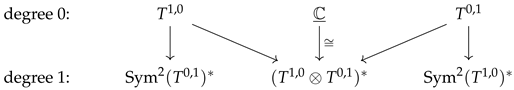 Here, the diagonal arrows are given by the divergence operator on smooth sections of the holomorphic or antiholomorphic tangent bundle. The outer vertical arrows are given by on the left and on the right, and the middle vertical arrow is multiplication by the background metric . Observing that this last arrow is an isomorphism, we can see that our model will be quasi-isomorphic—at least as a cochain complex—to one holomorphic and one anti-holomorphic copy of , as expected.
- 5.6.3. We exhibit a map of dg Lie algebras from to :
- A holomorphic vector field X is sent via the identity operator to the summand and via the negative of the divergence operator to the summand in .
- A Beltrami differential is sent to the antiholomorphic quadratic differential .
Both maps make use of the flat Kähler metric on the background geometry (or the corresponding volume form). Observe that the extra correction term along the summand corresponding to Weyl rescalings ensures that the terms in the differential proportional to cancel, so that is a cochain map.
To check that is a map of dg Lie algebras, it remains to check compatibility with the Lie bracket. There are two cases, one corresponding to two degree-zero generators, another corresponding to the action of a degree-zero generator on a degree-one generator. We proceed in order.
For the first, note that . This is to be compared with the bracket, in , of and . The latter, applying the definition, is , so things reduce to checking the identity
which can be derived quickly by applying the divergence operator to the BV identity for polyvector fields, or checked in coordinates if one prefers.
For the second, we observe that the bracket in between a smooth section of and an antiholomorphic quadratic differential is
On the other hand, the bracket between the function , viewed as a Weyl rescaling, and is . In total, we reproduce the Lie bracket between and the Beltrami differential , matching as we should.
- 5.6.4. Weyl and Virasoro cocycles. We now pull back the explicit cocycle
The Riemann curvature tensor has only one independent component in two dimensions, so it is sufficient for us to compute that
on the image of . Thus, the scalar curvature restricts to . The Euler density in two dimensions is the product of the scalar curvature with the metric volume form; the perturbation of the latter again restricts trivially along . Finally, restricting the generator of Weyl rescalings along sets it equal to . The result is
recovering precisely the local cocycle corresponding to the Virasoro central extension.
6. Observables and Currents
6.1. Motivating Example: Hamiltonian Mechanics
We recall the two dual roles that a Lie algebra can play with respect to a theory: Firstly, it can act on the theory as a group of symmetries. Secondly, it can play the role of a gauge invariance in the description of the physical states or field configurations of the theory. Two dual algebraic structures—“ghosts” and “currents”, if you will—witness these two roles. They are related by Koszul duality.
- 6.1.1. Infinitesimal symmetries of phase space. Let be a symplectic manifold. Recall that the space of symplectic vector fields on M is given by
Locally on M (or globally if M is simply connected), the Poincaré lemma shows that every closed one-form is exact. It, thus, lets us identify the space of closed one-forms with the space of functions, modulo the kernel of the de Rham operator, which just consists of constant functions. We can summarize these considerations by a short exact sequence
of sheaves of vector spaces, naturally defined on the site of all symplectic manifolds. (In light of the discussion above, the reader will hopefully see that the failure of the global sections of this sequence to be exact on certain manifolds M is due to the appearance of the higher sheaf cohomology group . In fact, after resolving the sheaf of closed one-forms, (83) is just (17) again!)
In fact, (83) is a short exact sequence of sheaves of Lie algebras. Here, locally constant functions are viewed as an abelian Lie algebra, symplectic vector fields are equipped with the obvious Lie bracket of vector fields, and the Lie algebra structure on observables (smooth functions on phase space) is defined by the Poisson bracket. We, thus, see that (83) witnesses observables as a one-dimensional central extension of symmetries. The center consists of locally constant functions on phase space: Physically, these are trivial observables that return no information about the system and, correspondingly, generate no nontrivial automorphism of the state space. The structure of this central extension is common to both classical mechanics and quantum mechanics.
For a Lie algebra, an action of on the phase space is defined by a map
of Lie algebras. Such an action induces a canonical central extension fitting into the following diagram:
We can imagine this central extension as the obstruction to lifting a symplectic action of on M to a Hamiltonian action.
Notice that the observables of a theory form a Poisson algebra: They have both a commutative algebra structure and a Lie bracket (the Poisson bracket), compatible in the sense that the adjoint action of the latter is by derivations of the former. The map at the middle term of this sequence, which is the moment map for the Hamiltonian action of on M, can similarly be extended to a map of Poisson algebras. Consider the symmetric algebra : It is a commutative algebra in obvious fashion, and we can extend the Lie bracket on the generators uniquely to a Poisson bracket on . A Hamiltonian action, thus, amounts to a map of Poisson algebras
which specializes the central element in to the numerical value of the anomaly in M. We think of this as a map from a universal Poisson algebra of currents for to the Poisson algebra of observables.
- 6.1.2. A word on quantization. For orientation, we offer a brief aside on quantization, which will probably be apparent to the reader anyway. One should think of a Poisson algebra as the “semiclassical residue” of a one-parameter family of associative algebras, parameterized by ℏ. The Poisson algebra we have constructed consists of (polynomial) functions on the linear space , equipped with the natural (Kirillov–Kostant–Souriau) Poisson bracket. Its quantization is just the universal enveloping algebra ; in quantum mechanics, we would have asked for a projective representation of on Hilbert space, which amounts to a map from to the algebra of linear operators. (Unitarity is, of course, important, but we will not discuss it here.)
- 6.1.3. Duality. There is an important sense in which the algebra of -currents and the algebra of -ghosts are dual to one another. The relationship is known as Koszul duality, and is witnessed by the fact that admits a differential that makes it quasi-isomorphic to the ground field. Morally speaking, the two factorization algebras we will soon associate to a local Lie algebra are also an instance of a Koszul dual pair. We do not have anything more specific to say about this here, but it is worth mentioning.
6.2. The Factorization Noether Theorem
We review the statement of Costello and Gwilliam’s Noether theorem for factorization algebras in a rough-and-ready manner, largely as encouragement for the reader to spend time with the discussion in ([1], Part III). Following this, we give some discussion of examples, hoping to build intuition for the statement.
- 6.2.1. We first give a schematic explanation to justify the shifts in cohomological degree appearing in the statement, which may be unfamiliar. Recall that the moduli space of fields in a BV theory is equipped with a -shifted symplectic structure . Correspondingly, modulo various subtleties, the observables should be equipped with a -shifted Poisson bracket. One expects a surjective map
Recalling our argument from above, we expect a symmetry by a Lie algebra to give rise to a commutative diagram of the shape
mirroring (85) above. Note that we now see a shifted central extension appearing, since constant observables sit in degree . Central extensions by any -module M are classified by the Lie algebra cohomology group , so we expect anomalies of this sort to be classified by
As the reader may recall, it is indeed the first cohomology group that appears in the classification of anomalies using BRST cohomology.
- 6.2.2. As we have seen above, a local Lie algebra defines a formal moduli problem, and a variational local Lie algebra defines a perturbative Lagrangian field theory. The observables are given by the factorization algebra
There is a dual factorization algebra that one can associate to a local Lie algebra. This factorization algebra, called the currents of , is defined by taking the cosheaf of compactly supported sections of and applying the covariant functor of Lie algebra chains. That is,
The structure here is inherited from the Lie bracket, and no restriction on the formal moduli problem is necessary. Just as quantization of produced the enveloping algebra , quantization of the current algebra produces a higher version of the enveloping algebra [69].
- 6.2.3. Noether’s theorem via descent. It deserves a bit of emphasis that the standard proof of Noether’s theorem already implicitly appeals to the structure of a derived replacement of the sheaf , namely, by the local Lie algebra controlling deformations of the trivial connection. In fact, even careful versions of the standard proofs appeal to a version of homological descent, but in the variational bicomplex rather than in a local resolution; the reader interested in learning more is referred to the careful discussion in ([70], §§2.6–8). We are not aware of any comparably careful treatment incorporating both spacetime descent and BV descent explicitly.
Recall that in the normal proofs, one “promotes a global symmetry to a local symmetry”. The fact that one knows how to do this unambiguously is a consequence of the fact that the symmetry acts locally: One actually had an action of on fields, rather than just of constant -valued functions. This accomplishes the first step of the replacement (16). By the general structure of a BV theory, one wants to witness this symmetry via a “moment map”, lifting along (87) to write down a map from to that shows how compactly supported symmetry transformations are generated by degree- observables under the BV bracket.
Since “the local symmetry was not a symmetry”, the variation of the action under the symmetry transformations is not zero. Consequently, the degree- observables we have written down are not closed with respect to the differential on observables in the BV theory, which encodes the equations of motion. But they must be closed when the gauge parameters are in fact constant: on the kernel of the differential in (16). Remembering the general structure of a resolution, this exactness should be explicitly witnessed by observables in degree zero; it is clear that the way to do this is simply to map the rest of the resolution (16) to the BV observables. We should, thus, expect a map from compactly supported one-forms valued in to degree-zero observables. These are nothing other than the standard Noether currents.
- 6.2.4. Visualizing the structure of . We now turn to seeing how this intuition is witnessed at the level of the factorization algebra of currents. Given a local Lie algebra, the generators of its currents are . It is useful for the intuition to recall that there is a pairing between compactly supported sections of the bundle L and distributional sections of . Here,
The utility of this maneuver lies in the fact that one is used to working with a description of the fields of a field theory; the observables are then generated by the dual of this space. If we want to understand currents as a “degenerate field theory” of sorts, it is useful to write down the would-be space of “fields”. The trick is exactly analogous to thinking of the Poisson algebra of currents as functions on a Poisson space ; here, we are giving a rough description of the currents of in terms of the observables of .
Writing out the structure explicitly, we see a complex of the form,
where we have used the physical convention for degrees, shifted down by one from the local Lie algebra grading: Physical fields are in degree zero. As we expected (and will see in examples in the following sections) the degree-zero portion of the current map corresponds to the standard Noether current, and the degree-one portion to its conservation law. Degree- generators of the currents induce equivalences between degree-zero currents; in the literature, such equivalence relations tend to be described as “improvement transformations.”
If an anomaly is present, we are interested in a central extension of by the constant sheaf . By now, though, the reader should see both an immediate problem with this example and its resolution. The sheaf is a sheaf of graded abelian Lie algebras, but is not a local Lie algebra. To get one, we must resolve it by the sheaf of de Rham forms, shifted by one. Including these generators into our diagram, we find a complex of the form
The top form in degree in the lower row corresponds to a class in , and is also responsible for the non-conservation of the current: the “anomalous Ward identity”. The form in degree zero, on the other hand, can be integrated over a sphere to give rise to a numerical anomaly in the form of an unshifted central extension of the sphere algebra.
- 6.2.5. Examples: global symmetries. Recall the three formal moduli problems extending the constant sheaf that we constructed above in Section 5.2. We visualize the structure of the currents for each as performed in the previous section. The currents for take the form
The currents for take the form
Note the appearance of -form improvement transformations in degree . Thinking about the standard form of the coupling terms in the Lagrangian, which is by the functional
these transformations reflect the fact that, under the assumption that A is a closed form, any shift of the current by an exact form shifts the coupling term by a total derivative and, thus, leaves the coupled action invariant. This would obviously not be true for general connections A.
Finally, the currents for take the form
Since the Hodge star interchanges exact forms with coexact forms, the resulting improvement transformations do not differ so dramatically from those for flat connections. Nevertheless, we emphasize that the set of improvement transformations is dictated by, and differs depending on, the exact local Lie algebra to which we choose to couple.
- 6.2.6. Examples: the stress tensor. The currents for the moduli problem of metrics take the form
None of these currents admit any nontrivial improvement transformation. The story one finds in textbooks, where the Noether currents for “global” translations give rise to a two-index stress tensor which must be “improved” to a symmetric one, only makes sense if one imagines a moduli problem corresponding to a de Rham-type resolution of constant sections of the tangent bundle. The geometric role of such a moduli problem in the story is unclear; after all, the thing that makes the translations into symmetries of a quantum field theory on flat space is not that they are constant, but that they are Killing vector fields with respect to the flat metric.
6.3. Disambiguation
We begin with a few remarks on terminology, which are intended to help avert confusion. These will veer into a recapitulation of the procedure of “gauging”, followed by some general philosophy and some far-fetched speculation.
- 6.3.1. Local symmetries versus gauge invariances. There is sometimes an unfortunate habit of conflating the term “local symmetry” with the term “gauge symmetry”. The term “local” is drastically overburdened in any case. For the purposes of disambiguation, we sketch the typical speech patterns, which (in our experience) are roughly as follows:
- Every symmetry of a field theory, or, at least, every infinitesimal symmetry, is tacitly assumed to act in a local manner. (Thus, it is encoded by an action of a sheaf of Lie algebras.) Whether or not a symmetry is called “local” has nothing to do with this.
- A symmetry by a locally constant sheaf of Lie algebras—in other words, a symmetry parameterized by functions that are constrained to be locally constant—is called a “global symmetry.”
- A symmetry by a locally free sheaf of Lie algebras—in other words, a symmetry parameterized by one or more unconstrained smooth functions—is called a “local symmetry.”
- A “gauge symmetry” is used to refer to a group action which, as in our cartoon in Section 2, is actually part of a presentation of the space of field configurations as a quotient of some other space.
- In standard situations, Noether’s second theorem [71] shows that symmetries of the action by a locally free sheaf of Lie algebras correspond one-to-one to nontrivial differential relations between the resulting variational equations of motion. When such relations are present, the variational principle does not define a well-defined boundary value problem. The typical remedy is to pass to studying the quotient space of the solutions by the corresponding local symmetry, which is, thus, invariably treated as a gauge invariance. This is the root cause of the tendency to conflate the two terms.
- Working with local Lie algebras offers a lot of clarity on many of these issues, but leads to new terminological complexities. In this article, I do my best to use language in a way that is, at least, largely internally consistent. Here are some principles of usage I hope I have managed to adhere to:
- 1:
- I will exclusively use the term “gauge symmetry” for the action of a group (or Lie algebra) appearing in a description of the sheaf of physical fields as a quotient. This is consistent with standard usage. The gauge symmetries of a theory are not a subset of its symmetries. Where possible, I will, thus, try and refer to “gauge invariances” rather than “gauge symmetries”, though I cannot promise consistency.
- 2:
- “Local” and “gauge” are distinct terms and are not to be equated. In particular, “local Lie algebra” is a general term with a fixed meaning (Definition 4) and does not bear any relation to the distinctions outlined above.
Taking invariants is a general procedure; correspondingly, any action of a group or Lie algebra may, or may not, appear playing the role of a gauge invariance. For example, in the case of a topologically or holomorphically twisted theory, one takes invariants of a fermionic symmetry that is “global” in the above sense. This is also performed in the context of “orbifolding” ([72], for example). On the other hand, Kac–Moody symmetry in two-dimensional conformal field theory is not “global”, since it is not locally constant, but is a symmetry and not a gauge invariance.
- 6.3.2. The dogma of the ghost in the machine. It is common in expositions of the BRST formalism to emphasize that the ghost fields that one introduces are “a trick”, or perhaps (in some vague sense of the word) “formal”—in any case, certainly “unphysical”. While the narrow point that is being made is not wrong, the would-be ontology that lies behind it is misleading and breeds confusion down the road. (The reader who has time to spare might investigate ([73], §1.2).)
The cohomology of a formal moduli problem in degree zero has a clear meaning: It classifies the symmetries of the background configuration, just as the Maurer–Cartan elements (in degree one) classify its perturbative deformations. Correspondingly, the local Lie algebras describing field theories of physical interest can, and do, often have cohomology in degree zero (“ghost number one”). Even the simplest example, perturbative abelian Yang–Mills theory, does: Locally constant gauge transformations appear there as a physical symmetry. Additionally, one knows such a symmetry has to be present: After all, the electric charge is measurable, and states of nonzero electric charge exist in QED—even though the symmetry has been “gauged.”
More broadly, Dogma 1 tells us that we are forced to think about objects together with their (auto)equivalences to understand gauge theory, and we certainly believe that gauge theories appear in nature. Of course there may be many different equivalent models of the same gauge theory, just as there are many different equivalent triangulations of a space or many different equivalent resolutions of a sheaf. A gauge theory may even sometimes be equivalent to a non-gauge theory, in the manner that a quotient of one space may be isomorphic to a subspace of some other space. But in any given description, the ghosts—being a description of the (auto)equivalences—are part of a specification of the field content. They are as necessary and as “real” as any other part of that specification, even though we do not measure numerical values for them.
- 6.3.3. Gauging. Recall that actions of a Lie algebra on another Lie algebra correspond to split extensions of the form
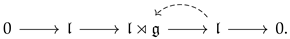
The steps that one performs in “gauging” a symmetry (which is usually imagined to be a “global” symmetry) are the following:
- 1:
- Formulate the symmetry in terms of a local Lie algebra . When the symmetry is by a locally constant sheaf of Lie algebras , is typically the moduli problem of G-connections.
- 2:
- Identify a -shifted symplectic formal moduli problem that maps to .
- 3:
- The semidirect product is now itself a variational formal moduli problem, representing the total space of the fibration. After gauging, we study this formal moduli problem, regarding it as a theory in and of itself.
The original formal moduli problem in this description does not play any essential role, and we could have omitted it. The important thing is to choose a variational formal moduli problem that acts on another variational formal moduli problem. A sketch of this procedure is in Figure 1.
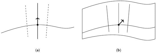
Figure 1.
The procedure of gauging a symmetry. (a) Before gauging, we study the moduli of deformations of the basepoint within the fiber, equivariantly as a family over the base. (b) After gauging, we study the moduli of deformations of the basepoint within the total space of the family.
- 6.3.4. Completeness (no global symmetries). In the context of recent attempts to axiomatize the properties of the set of low-energy effective field theories that can arise under the assumption of a consistent coupling to gravity, there has been much discussion of the conjectured absence of global symmetries. In the context of string theory, this absence is well established, originating as a “folk theorem” known, at least, to ’t Hooft, Susskind, and Witten, and seemingly first discussed in the literature in [74]. General arguments connecting black holes to global symmetry violation go back even further [75].
In perturbative quantum field theory, we can try and parse similar statements at the level of the relevant formal moduli problems. As we have seen, symmetries of a semiclassical perturbative field theory are represented by actions of one local Lie algebra (representing the symmetry) on another (representing the field theory) by outer automorphisms. Recall that, for any Lie algebra , there is a canonical four-term exact sequence of Lie algebras of the form
The middle arrow just sends to the endomorphism of ; by definition, the kernel of this map is the center of , and the cokernel is the Lie algebra of (infinitesimal) outer automorphisms. A Lie algebra is called complete when this arrow is an isomorphism, so that is centerless and has no nontrivial (infinitesimal) outer automorphisms.
Idea 2
(“No prior geometry.”). A complete quantum field theory should be a variational moduli problem on the site of smooth manifolds, defined without reference to any background local structure. A complete perturbative quantum field theory should be represented by a local Lie algebra that is, in an appropriate sense, complete.
Other than the last sentence, there is nothing new about this way of formulating the idea; it goes back, in some form, to Einstein. For the origin of the phrase we use here, we refer to a lucid remark in the classic treatise ([76], p. 431):
Mathematics was not sufficiently refined in 1917 to cleave apart the demands for “no prior geometry” and for a geometric, coordinate-independent formulation of physics. Einstein described both demands by a single phrase, “general covariance”. The “no prior geometry” demand actually fathered general relativity, but by doing so anonymously, disguised as “general covariance”, it also fathered half a century of confusion.
In our discussion of the étale site above, we used the term “general covariance” as a gloss, referring to the requirement of functoriality with respect to structure-preserving local isomorphisms. This is the narrower (and, from a geometric perspective, the less contentful) of the two meanings that Einstein had, but it feels less confusing to us to interpret an ambiguous phrase in the narrowest possible manner. The use of “general covariance” for the broader principle is widespread: For an example, the reader is referred to the discussion in the introduction of [77].
What we wish to emphasize here is that the origin of the idea that the metric should be dynamical was a principle—all background geometric structures should be dynamically determined—that equally well applies to other global symmetries. A theory with a global symmetry is nothing other than a theory defined over the family of (some class of) connections in a chosen principal G-bundle, and such a datum is certainly geometric. Since the principle of the absence of global symmetry is the same as the principle of no prior geometry, one should, perhaps, really attribute it to Einstein….
This principle is borne out naturally in string theory, where it has been well known for a long time that there are “no free parameters”. The intuition is perhaps the sharpest in the context of topological string theory. (I thank Surya Raghavendran, in particular, for many illuminating related discussions.) In modern descriptions [78], a topological string theory background is specified by describing its category of branes, which is a Calabi–Yau category. The open string field theories describing the degrees of freedom on a brane are then computed as the formal moduli problem of deformations of that brane, while the closed string field theory is computed via cyclic cohomology and gives a description of the formal moduli problem of deformations of the category itself. In general, one expects that those formal moduli problems that arise from a “first-quantized” description are precisely the formal moduli problems, where n is the dimension of the worldvolume; to say that a field theory is a closed-string field theory should be to say that it admits the structure of an moduli problem.
As a result of these considerations, we obtain a potential strategy of rigorous proof (or disproof) for perturbative versions of “string universality” statements, which would go roughly as follows:
- 1:
- Carefully formulate a well-defined notion of “completeness” for local Lie algebras, and understand its meaning for the corresponding formal moduli problems. (They should, in some sense, not occur as the fiber of any nontrivial family over another formal moduli problem on the site of manifolds.)
- 2:
- Argue that any complete local Lie algebra does, in fact, describe an formal moduli problem. Alternatively, identify a set of sufficient conditions for this to be the case, or identify an obstruction to the existence of an structure.
We look forward to thinking about such ideas in the future.
7. Higher Virasoro Algebras in Supersymmetric Theories
7.1. Minimal Conformal Supergravity in Four Dimensions
We show explicitly, using a component-field description, how the twist of the moduli problem of four-dimensional superconformal structures—in an arbitrary background admitting such a twist—reduces to the moduli problem of complex structures. We also review how the anomalies match up, following recent work of Williams and sketching how this goes at the component level.
- 7.1.1. Let M be a smooth oriented four-manifold, and let denote its complexified tangent bundle. We fix two complex vector bundles on M, denoted , together with an isomorphism
The isomorphism gives rise to isomorphisms of the form
for the symmetric square of the tangent bundle, and
for the endomorphism bundle of the tangent bundle.
- 7.1.2. Denote the Chern roots of the bundles by and , respectively. The Chern roots of the bundle are, then,
- 7.1.3. A choice of superconformal structure of type determines a reduction in the structure group to ; the corresponding principal bundle is the bundle of adapted frames. (For early work on G-structures on supermanifolds and adapted frames, see [79,80].) For structures in four dimensions, the corresponding reduction in the structure group is along the map
We observe that the map also has a kernel: As such, a reduction in the structure group along this map includes a choice of principal -bundle, the R-symmetry bundle, together with a reduction in the structure group to . Working with the Euclidean real form, this group would be , corresponding to a conformal structure on M.
- 7.1.4. To perform the twist, we first put a -graded structure on our supermanifold, placing in cohomological degree and in cohomological degree . The theory admits a holomorphic twist precisely when one of the two bundles—say , to conform to our choice of regrading—admits a globally nonvanishing section. This means that splits as a sum of lines
We further note that the tangent bundle decomposes as
Since is trivial, the second summand is isomorphic to , but an isomorphism is only given after choosing a trivialization: a volume form on M. The theory is independent of such a datum, and we will not make use of it.
- 7.1.5. A choice of splitting of as a sum of lines implies a further reduction of the structure group, and fixing a section of the trivial sub-line (a twisting supercharge) reduces down to
- 7.1.6. Following [9], the underlying vector bundle of the moduli problem of four-dimensional superconformal structures takes the form
After twisting, we obtain a -graded local Lie algebra (since the result has purely even intrinsic parity). The result is described in Table 1. In that table, we maintain the convention as to columns adopted in (112). Generators that survive the twist are circled, and the portions of the holomorphic supercharge that act acyclically by order-zero differential operators are indicated with the dashed arrows that proceed down and to the left. The portions of the holomorphic supercharge that act via spacetime derivatives are not shown explicitly; they would act down and to the right, inducing (among other things) differentials between generators in degrees one and two.

Table 1.
Twisting conformal supergravity.
- 7.1.7. We observe that the generators that survive the twist correspond precisely to the generators of the Dolbeault resolution of holomorphic vector fields, which is given by the dg Lie algebra . Generators in degree zero arise from the holomorphic part of the smooth vector fields that implement the quotient by diffeomorphisms in the original moduli problem (112).
In degree one, generators of the holomorphic formal moduli problem correspond to Beltrami differentials, or infinitesimal deformations of complex structure. With respect to (the conformal class of) a Kähler metric, these tensors decompose into a rank-three subbundle (corresponding to holomorphic quadratic differentials) and a rank-one subbundle (corresponding to deformations of the complex structure that are compatible with a deformed Kähler metric in the same conformal class). With respect to our model, the former come from trace-free metric perturbations, while the latter are represented by a component of the ghost field for local supersymmetry: We emphasize, though, that statements of this kind are model-dependent. As such, they are not especially meaningful, even if sometimes useful for the intuition. If we had used a description of the untwisted formal moduli problem that contained the trace part of the metric perturbations as a component field, we would have found it representing the same cohomology class in the twist.
Lastly, the generators in degree two arise from components of the gravitino field. We, thus, see that the Maurer–Cartan equation for deformations of complex structure arises from the condition of compatibility with supersymmetry. By contrast, perturbations of the conformal class of a metric obey no particular constraint.
7.2. Anomalies and Cocycles
By way of closure, we use the twist computation above to briefly indicate the connection between the conformal anomaly and the higher Virasoro anomaly at a schematic level.
- 7.2.1. In four dimensions, there are two independent anomaly cocycles in . The a cocycle is defined by the product of the ghost for Weyl rescaling with the Euler density, evaluated on the deformed metric . In this dimension, the Euler density is quadratic in the Ricci curvature. For the c cocycle, the Euler density is replaced by the square of the conformally invariant Weyl tensor of .
Working on flat space, we imagine a computation in which g is the flat metric. The lowest-order terms in h in the Taylor expansion of the Riemann curvature tensor are proportional to second derivatives of h. As such, the lowest term in either cocycle involves some combination of two second derivatives of the metric perturbation.
Remembering the computation in Section 5.6 and comparing it to the cohomology computation in Section 7.1, it is clear that the map that sends to the twist of will send a holomorphic vector field to the Weyl ghost via the divergence operator, and will send a Beltrami differential to a portion of the metric. The higher Virasoro cocycle contains a term of the form
ignoring contractions of indices. This term has one derivative of a vector field and two second derivatives of Beltrami differentials and, thus, has precisely the right form to arise from the pullback of a conformal anomaly cocycle. For details about the precise relation of the higher Virasoro algebra to the supersymmetrizations of the a and c anomalies, we refer to [64].
Funding
This work is funded by the Deutsche Forschungsgemeinschaft (DFG, German Research Foundation) under Projektnummer 517493862 (Homologische Algebra der Supersymmetrie: Lokalität, Unitarität, Dualität), and further by the Free State of Bavaria.
Data Availability Statement
Data sharing is not applicable to this article.
Conflicts of Interest
The author declares no conflicts of interest.
References
- Costello, K.; Gwilliam, O. Factorization Algebras in Quantum Field Theory II; Number 41 in New Mathematical Monographs; Cambridge University Press: Cambridge, UK, 2021. [Google Scholar]
- Pantev, T.; Toën, B.; Vaquié, M.; Vezzosi, G. Shifted symplectic structures. Publ. Mathématiques de l’IHÉS 2013, 117, 271–328. [Google Scholar] [CrossRef]
- Vakil, R. The Rising Sea; Princeton University Press: Princeton, NJ, USA, 2024. [Google Scholar]
- Hamilton, W.R. On a General Method of Expressing the Paths of Light, & of the Planets, by the Coefficients of a Characteristic Function; P. Dixon Hardy: Dublin, Ireland, 1833. [Google Scholar]
- Costello, K.; Gwilliam, O. Factorization Algebras in Quantum Field Theory I; Number 31 in New Mathematical Monographs; Cambridge University Press: Cambridge, UK, 2017. [Google Scholar]
- Freed, D.S. Lectures on topological quantum field theory. In Proceedings of the GIFT Summer School on Recent Problems in Mathematical Physics, Salamanca, Spain, 15–27 June 1992. [Google Scholar]
- Freed, D.S.; Hopkins, M. Chern–Weil forms and abstract homotopy theory. Bull. Am. Math. Soc. 2013, 50, 431–468. [Google Scholar] [CrossRef]
- Freed, D.S. What is an anomaly? arXiv 2023, arXiv:2307.08147. [Google Scholar]
- Hahner, F.; Raghavendran, S.; Saberi, I.; Williams, B.R. Local superconformal algebras. arXiv 2024, arXiv:2410.08176. [Google Scholar] [CrossRef]
- Mac Lane, S. Categories for the Working Mathematician, 2nd ed.; Number 5 in Graduate Texts in Mathematics; Springer: Berlin/Heidelberg, Germany, 2013. [Google Scholar]
- Coecke, B.; Paquette, E.O. Categories for the practicing physicist. In New Structures for Physics; Coecke, B., Ed.; Number 813 in Lecture Notes in Physics; Springer: Berlin/Heidelberg, Germany, 2010; pp. 173–286. [Google Scholar]
- Behrend, K.; Xu, P. Differentiable stacks and gerbes. J. Symplectic Geom. 2011, 9, 285–341. [Google Scholar] [CrossRef]
- Milne, J.S. Lectures on Étale Cohomology; Number 33 in Princeton Mathematical Series; Princeton University Press: Princeton, NJ, USA, 1980. [Google Scholar]
- Manin, Y.I. Gauge Field Theory and Complex Geometry; Number 289 in Grundlehren der mathematischen Wissenschaften; Springer: Berlin/Heidelberg, Germany, 1984. [Google Scholar]
- Deligne, P. Superspace approaches to supergravity. In Quantum Fields and Strings: A Course for Mathematicians; Deligne, P., Etingof, P., Freed, D.S., Jeffrey, L.C., Kazhdan, D., Morgan, J.W., Morrison, D.R., Witten, E., Eds.; American Mathematical Society: Providence, RI, USA, 1999; Volume 2. [Google Scholar]
- Giraud, J. Analysis Situs; Number 256 in Séminaire Bourbaki 1962/63; Secrétariat Mathématique, Université Paris: Paris, France, 1964. [Google Scholar]
- Aharonov, Y.; Bohm, D. Significance of electromagnetic potentials in the quantum theory. Phys. Rev. 1959, 115, 485. [Google Scholar] [CrossRef]
- Tonomura, A.; Osakabe, N.; Matsuda, T.; Kawasaki, T.; Endo, J.; Yano, S.; Yamada, H. Evidence for Aharonov–Bohm effect with magnetic field completely shielded from electron wave. Phys. Rev. Lett. 1986, 56, 792–795. [Google Scholar] [CrossRef] [PubMed]
- Godement, R. Topologie Algébrique et Théorie des Faisceaux; Number 13 in Publications de l’Institut de Mathématique de l’Université de Strasbourg; Hermann: Paris, France, 1958. [Google Scholar]
- Bredon, G.E. Sheaf theory. In Graduate Texts in Mathematics; Springer: Berlin/Heidelberg, Germany, 2012; Volume 170. [Google Scholar]
- Swan, R.G. Vector bundles and projective modules. Trans. Am. Math. Soc. 1962, 105, 264–277. [Google Scholar] [CrossRef]
- Weil, A. Sur les théorèmes de de Rham. Comment. Math. Helv. 1952, 26, 119–145. [Google Scholar] [CrossRef]
- Chevalley, C.; Eilenberg, S. Cohomology theory of Lie groups and Lie algebras. Trans. Am. Math. Soc. 1948, 63, 85–124. [Google Scholar] [CrossRef]
- Becchi, C.; Rouet, A.; Stora, R. Renormalization of the abelian Higgs–Kibble model. Commun. Math. Phys. 1975, 42, 127–162. [Google Scholar] [CrossRef]
- Tyutin, I.V. Gauge invariance in field theory and statistical physics in operator formalism. Lebedev Phys. Inst. 1975, 39. [Google Scholar]
- Deligne, P.; Morgan, J.W. Notes on supersymmetry (following Joseph Bernstein). In Quantum Fields and Strings: A Course for Mathematicians; Deligne, P., Etingof, P., Freed, D.S., Jeffrey, L.C., Kazhdan, D., Morgan, J.W., Morrison, D.R., Witten, E., Eds.; American Mathematical Society: Providence, RI, USA, 1999; Volume 1, pp. 41–98. [Google Scholar]
- Raghavendran, S.; Saberi, I.; Williams, B.R. Twisted eleven-dimensional supergravity. Commun. Math. Phys. 2023, 402, 1103–1166. [Google Scholar] [CrossRef]
- Manetti, M. Differential graded Lie algebras and formal deformation theory. In Algebraic Geometry: Seattle 2005; Number 80 in Proceedings of Symposia in Pure Mathematics; AMS: Amsterdam, The Netherlands, 2009; pp. 785–810. [Google Scholar]
- Atiyah, M.F.; MacDonald, I.G. Introduction to Commutative Algebra; Westview Press: Boulder, CO, USA, 1969. [Google Scholar]
- Vezzosi, G. What is …a derived stack? Not. Am. Math. Soc. 2011, 58, 955–958. [Google Scholar]
- The Stacks Project: An Open Source Textbook and Reference Work on Algebraic Geometry. Available online: https://stacks.math.columbia.edu (accessed on 4 July 2025).
- Lurie, J. Derived Algebraic Geometry X: Formal Moduli Problems. Available online: https://www.math.ias.edu/~lurie/papers/DAG-X.pdf (accessed on 4 July 2025).
- Quillen, D. Rational homotopy theory. Ann. Math. 1969, 90, 205–295. [Google Scholar] [CrossRef]
- Sullivan, D. Infinitesimal computations in topology. Publ. Mathématiques de l’IHÉS 1977, 47, 269–331. [Google Scholar] [CrossRef]
- Kodaira, K.; Spencer, D.C. On deformations of complex analytic structures, I–II. Ann. Math. 1958, 67, 328–466. [Google Scholar] [CrossRef]
- Nijenhuis, A.; Richardson, R.W., Jr. Cohomology and deformations in graded Lie algebras. Bull. Am. Math. Soc. 1966, 72, 1–29. [Google Scholar] [CrossRef]
- Deligne, P. Letter to John Millson. 1987. Available online: https://publications.ias.edu/sites/default/files/millson.pdf (accessed on 4 July 2025).
- Drinfeld, V. A letter from Kharkov to Moscow (1988). Ems Surv. Math. Sci. 2014, 1, 241–248. [Google Scholar] [CrossRef]
- Pridham, J.P. Unifying derived deformation theories. Adv. Math. 2010, 224, 772–826. [Google Scholar] [CrossRef]
- Hinich, V. DG coalgebras as formal stacks. J. Pure Appl. Algebra 2001, 162, 209–250. [Google Scholar] [CrossRef]
- Getzler, E. Lie theory for nilpotent L∞ algebras. Ann. Math. 2009, 170, 271–301. [Google Scholar] [CrossRef]
- Calaque, D.; Grivaux, J. Formal moduli problems and formal derived stacks. Panoramas Synthèses 2021, 55, 85–145. [Google Scholar]
- Vallette, B. Algebra + homotopy = operad. Symplectic Poisson. Noncommut. Geom. 2014, 62, 229–290. [Google Scholar]
- Batalin, I.A.; Vilkovisky, G.A. Gauge algebra and quantization. Phys. Lett. B 1981, 102, 27–31. [Google Scholar] [CrossRef]
- Batalin, I.A.; Vilkovisky, G.A. Closure of the gauge algebra, generalized Lie equations, and Feynman rules. Nucl. Phys. B 1984, 234, 106–124. [Google Scholar] [CrossRef]
- Batalin, I.A.; Vilkovisky, G.A. Existence theorem for gauge algebra. J. Math. Phys. 1985, 26, 172–184. [Google Scholar] [CrossRef]
- Wess, J.; Zumino, B. Consequences of anomalous Ward identities. Phys. Lett. B 1971, 37, 95–97. [Google Scholar] [CrossRef]
- Bonora, L.; Cotta-Ramusino, P. Some remarks on BRS transformations, anomalies, and the cohomology of the Lie algebra of the group of gauge transformations. Commun. Math. Phys. 1983, 87, 589–603. [Google Scholar] [CrossRef]
- Barnich, G.; Brandt, F.; Henneaux, M. Local BRST cohomology in gauge theories. Phys. Rep. 2000, 338, 439–569. [Google Scholar] [CrossRef]
- Bertlmann, R.A. Anomalies in Quantum Field Theory; Number 91 in International Series of Monographs on Physics; Oxford University Press: Oxford, UK, 2000. [Google Scholar]
- Bonora, L. Fermions and Anomalies in Quantum Field Theories; Theoretical and Mathematical Physics; Springer: Berlin/Heidelberg, Germany, 2023. [Google Scholar]
- Adler, S.L. Axial-vector vertex in spinor electrodynamics. Phys. Rev. 1969, 177, 2426. [Google Scholar] [CrossRef]
- Bell, J.S.; Jackiw, R.W. A PCAC puzzle: π0→ γγ in the σ-model. Il Nuovo C. A 1969, 60, 47–61. [Google Scholar] [CrossRef]
- Brylinski, J.L. Loop Spaces, Characteristic Classes, and Geometric Quantization; Number 107 in Progress in Mathematics; Springer: Berlin/Heidelberg, Germany, 2009. [Google Scholar]
- Saberi, I.; Williams, B.R. Constraints in the BV formalism: Six-dimensional supersymmetry and its twists. Adv. Math. 2023, 412, 108806. [Google Scholar] [CrossRef]
- Butson, D.; Yoo, P. Degenerate classical field theories and boundary theories. arXiv 2016, arXiv:1611.00311. [Google Scholar]
- Bonora, L.; Cotta-Ramusino, P.; Reina, C. Conformal anomaly and cohomology. Phys. Lett. B 1983, 126, 305–308. [Google Scholar] [CrossRef]
- Bonora, L.; Pasti, P.; Bregola, M. Weyl cocycles. Class. Quantum Gravity 1986, 3, 635. [Google Scholar] [CrossRef]
- Deser, S.; Schwimmer, A. Geometric classification of conformal anomalies in arbitrary dimensions. Phys. Lett. B 1993, 309, 279–284. [Google Scholar] [CrossRef]
- Boulanger, N. General solutions of the Wess–Zumino consistency condition for the Weyl anomalies. J. High Energy Phys. 2007, 2007, 069. [Google Scholar] [CrossRef]
- Gwilliam, O.; Williams, B.R. Higher Kac–Moody algebras and symmetries of holomorphic field theories. Adv. Theor. Math. Phys. 2021, 25, 129–239. [Google Scholar] [CrossRef]
- Faonte, G.; Hennion, B.; Kapranov, M. Higher Kac–Moody algebras and moduli spaces of G-bundles. Adv. Math. 2019, 346, 389–466. [Google Scholar] [CrossRef]
- Saberi, I.; Williams, B.R. Twisted characters and holomorphic symmetries. Lett. Math. Phys. 2020, 110, 2779–2853. [Google Scholar] [CrossRef]
- Williams, B.R. A complex geometric perspective on the a and c anomalies. arXiv 2024, arXiv:2404.16128. [Google Scholar] [CrossRef]
- Williams, B.R. The local cohomology of vector fields. arXiv 2024, arXiv:2405.05174. [Google Scholar] [CrossRef]
- Gel’fand, I.M.; Fuks, D.B. Cohomology of the Lie algebra of formal vector fields. Math. USSR–Izvestiya 1970, 4, 327. [Google Scholar] [CrossRef]
- Bott, R. On characteristic classes in the framework of Gelfand–Fuks cohomology. Astérisque 1976, 32–33, 113–139. [Google Scholar]
- Gel’fand, I.M.; Fuks, D.B. The cohomologies of the Lie algebra of the vector fields in a circle. Funct. Anal. Appl. 1968, 2, 342–343. [Google Scholar] [CrossRef]
- Knudsen, B. Higher enveloping algebras. Geom. Topol. 2018, 22, 4013–4066. [Google Scholar] [CrossRef]
- Deligne, P.; Freed, D.S. Classical field theory. In Quantum Fields and Strings: A Course for Mathematicians; Deligne, P., Etingof, P., Freed, D.S., Jeffrey, L.C., Kazhdan, D., Morgan, J.W., Morrison, D.R., Witten, E., Eds.; American Mathematical Society: Providence, RI, USA, 1999; Volume 1, pp. 137–226. [Google Scholar]
- Noether, E. Invariante Variationsprobleme. Nachrichten Ges. Wiss. Göttingen Math.-Phys. Kl. 1918, 1918, 235–257. [Google Scholar]
- Brunner, I.; Carqueville, N.; Plencner, D. Orbifolds and topological defects. Commun. Math. Phys. 2014, 332, 669–712. [Google Scholar] [CrossRef]
- Ryle, G. The Concept of Mind; Hutchinson: London, UK, 1949. [Google Scholar]
- Banks, T.; Dixon, L.J. Constraints on string vacua with spacetime supersymmetry. Nucl. Phys. B 1988, 307, 93–108. [Google Scholar] [CrossRef]
- Zeldovich, Y.B. A new type of radioactive decay: Gravitational annihilation of baryons. Phys. Lett. A 1976, 59, 254. [Google Scholar] [CrossRef]
- Misner, C.W.; Thorne, K.S.; Wheeler, J.A. Gravitation; Macmillan: New York, NY, USA, 1973. [Google Scholar]
- Witten, E. Quantum field theory and the Jones polynomial. Commun. Math. Phys. 1989, 121, 351–399. [Google Scholar] [CrossRef]
- Costello, K. Topological conformal field theories and Calabi–Yau categories. Adv. Math. 2007, 210, 165–214. [Google Scholar] [CrossRef]
- Schwarz, A.S. Supergravity, complex geometry, and G-structures. Commun. Math. Phys. 1982, 87, 37–63. [Google Scholar] [CrossRef]
- Fujio, M. Super G-structures of finite type. Osaka J. Math. 1991, 28, 163–211. [Google Scholar]
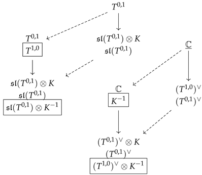
Disclaimer/Publisher’s Note: The statements, opinions and data contained in all publications are solely those of the individual author(s) and contributor(s) and not of MDPI and/or the editor(s). MDPI and/or the editor(s) disclaim responsibility for any injury to people or property resulting from any ideas, methods, instructions or products referred to in the content. |
© 2025 by the author. Licensee MDPI, Basel, Switzerland. This article is an open access article distributed under the terms and conditions of the Creative Commons Attribution (CC BY) license (https://creativecommons.org/licenses/by/4.0/).