Distributed Time Delay Models: An Alternative to Fractional Calculus-Based Models for Fractional Behavior Modeling

Abstract

This paper illustrates that distributed time delay models can exhibit fractional behaviors, addressing the limitations of fractional calculus-based models outlined in the introduction. Given the extensive results generated by these models, they present a compelling alternative to fractional models. The demonstration is done both in discrete time and in continuous time. The two cases yield fractional behavior within a defined time/frequency range. To conclude and using two examples, the article highlights that modeling fractional behaviors using distributed delay systems allows for coherent physical interpretations, which a fractional model representation struggles to achieve.

1. Introduction

Since the seminal work of Mandelbrot [1], it has been established that natural phenomena frequently adhere to fractal geometries. While the prevalence of fractality in geometric contexts may seem to be a static characteristic, this perception is misleading. Certain physical processes give rise to fractals, and the dynamics involved in their formation and progression exhibit distinct behaviors [2,3]. These dynamics are governed by power laws, often referred to as fractional behaviors [4,5]. For example, classical diffusion processes demonstrate 1/2 fractional behaviors due to the presence of fractal diffusion fronts [3]. Numerous other phenomena could be referenced in this context [5]. When these physical processes occur within dynamical systems, they impose a fractional dynamic behavior on the system. This is particularly evident in electrochemical devices [6], various biological systems [7], thermal systems [8], viscoelastic materials [9], and numerous other systems.

Fractional dynamic behaviors are frequently modeled and analyzed through fractional models [10], which are defined by differential equations where traditional derivatives are substituted with fractional derivatives [11]. However, this approach lacks a theoretical foundation. The sole justification for its use is that fractional integration and differentiation operators exhibit fractional characteristics.

Does fractional calculus provide solutions? While models based on fractional calculus have demonstrated impressive fitting capabilities, they often fail to yield a coherent physical interpretation of the systems under examination. Moreover, the application of fractional calculus in defining fractional models introduces certain limitations and inconsistencies in physical interpretation [12,13,14,15], particularly when initial conditions are considered [16] and if Caputo’s definition is used [17]. Despite the widespread popularity of these models, which have resulted in numerous publications and generalizations, a critical analysis reveals that many methodologies for modeling fractional behaviors were already present in the literature prior to the surge of interest in fractionalization—characterized by the tendency to create fractional counterparts of classical integer models. It is indeed feasible to capture fractional behaviors effectively, often under more favorable conditions, through the use of the following:

-

Convolution models with various non-singular kernels [18,19];

-

Diffusive representations [20,21];

-

Certain classes of nonlinear models [22,23];

-

Specific types of time-varying models [24,25];

-

Peridynamic models [26];

-

Partial differential equations with spatially distributed coefficients [27].

The first two have been widely considered in the literature. A large number of studies have been devoted to convolution models with various non-singular kernels in recent years because they allow us to remove a constraint imposed by fractional calculus and models: singular kernels in the operator definitions. Lifting this constraint is not done to the detriment of the effectiveness of these models to generate fractional behaviors (and therefore capture them), since from a physical point of view, fractional behaviors are not on asymptotic domains. Regarding diffusive representations, it has the merit of revealing the doubly infinite dimension of the state [16] of fractional operators and models (at the origin of the physical inconsistencies of certain works) and leads to the emergence of the Infinite State Representation [17]. However, it is defined as a time constant distribution, which is already a macro representation which moves away from the physical phenomena that induce fractional behaviors.

This study examines another alternative class of models. Following an initial exploration in [28], it is demonstrated that distributed time delay models possess a significant capacity to produce fractional behaviors, thereby positioning them as viable candidates for modeling such phenomena. In contrast to [28], this work addresses the discrete time case, which is not covered in [28]. For the continuous time case, new conditions on the parameters of the examined distributed time delay models are established to achieve fractional behaviors. The resulting frequency response exhibits a low-pass characteristic, which was not observed in [28], making it now more physically realistic. Additionally, a different class of kernel is utilized to define the model. The underlying physical mechanisms that enable distributed delay models to manifest fractional behaviors are also scrutinized. Indeed, by further investigating the origins of fractional behaviors introduced earlier in this section, it becomes evident that these behaviors stem not only from a connection to fractality but also from the sequential interactions of numerous agents within a constrained environment—one that is limited by the fractal being formed or that already exists in the spatial context of the phenomenon. Consequently, the concept of distributed delay is fully realized, exemplified by the delays experienced by particles as they navigate the process of diffusion or as they seek to occupy positions on an adsorbent surface.

This paper is organized as follows. Section 2 recalls strictly necessary definitions on fractional calculus and fractional models. A first proof of the ability of distributed time delay models to produce fractional behaviors is given in Section 3 for the discrete time case. This demonstration is based on the Grünwald–Letnikov definition for a fractional differentiation operator. A similar demonstration is done in the continuous time case in Section 4. It first introduces an approximation of fractional differentiation operator using a non-singular kernel. Section 5 finally highlights that the distributed time delay models allow coherent physical interpretations of the phenomena that generate fractional behaviors.

2. Fractional Calculus and Fractional Models: A Reminder

The fractional integral of order $\nu$, $\nu \in {ℝ}_{+}$, of a function $z\left(t\right)$ is defined by [11]:

$${\mathit{I}}_{t_0}^{\nu }\left[z\left(t\right)\right]={\displaystyle \frac{1}{\Gamma \left(\nu \right)}}{{\displaystyle \int }}_{t_0}^t{\displaystyle \frac{z\left(\tau \right)}{{\left(t-\tau \right)}^{1-\nu }}}d\tau$$

(1)

$\Gamma \left(.\right)$ being Euler’s gamma function. Regarding fractional differentiation, the situation is more complex. Various definitions (at least 30) can be used to describe this operator [29], which raises the question of choice. These definitions are in certain respects equivalent, but differences exist, notably regarding how initial conditions are taken into account.

In the Riemann–Liouville sense, the fractional derivative of order $\nu$, $m-1<\nu <m$, $m\in {\mathbb{N}}_{+}^{*}$, of a function $z\left(t\right)$ is defined by [30]:

$${\mathit{D}}_{t_0}^{\nu }\left[z\left(t\right)\right]={\displaystyle \frac{d^m}{d{t}^m}}\left({\mathit{I}}_{t_0}^{m-\nu }z\left(t\right)\right)={\displaystyle \frac{d^m}{d{t}^m}}\left({\displaystyle \frac{1}{\Gamma \left(m-\nu \right)}}{{\displaystyle \int }}_{t_0}^t{\displaystyle \frac{z\left(\tau \right)}{{\left(t-\tau \right)}^{1-m+\nu }}}d\tau \right)$$

(2)

To address the problem of discretizing these operators, the Grünwald–Letnikov definition [31,32] is very often used. This definition is given by

$${\mathit{D}}_{t_0}^{\nu }\left[z\left(t\right)\right]=\underset{h\to 0}{\lim }\left[{\displaystyle \frac{1}{h^{\nu }}}{\displaystyle \sum }_{k=0}^{\infty }\gamma \left(\nu ,k\right)z\left(t-t_0-kh\right)\right]$$

(3)

with

$$\gamma \left(\nu ,k\right)={\left(-1\right)}^k{\displaystyle \frac{\Gamma \left(\nu +1\right)}{k!\Gamma \left(\nu -k+1\right)}}$$

(4)

Using these definitions, if $u\left(t\right)\in ℝ$ and $y\left(t\right)\in ℝ$ respectively denote input and output signals, a fractional differential equation is found in the literature with the form:

$${\displaystyle \sum }_{k=0}^{N_a}{a}_k{\mathit{D}}_{t_0}^{{\nu }_{a_k}}\left[y\left(t\right)\right]={\displaystyle \sum }_{k=0}^{N_b}{b}_k{\mathit{D}}_{t_0}^{{\nu }_{b_k}}\left[u\left(t\right)\right]$$

(5)

In relation (5), $a_k\in ℝ$ and $b_k\in ℝ$. ${\mathit{D}}_{t_0}^{{\nu }_{a_k}}$ and ${\mathit{D}}_{t_0}^{{\nu }_{b_k}}$ denote, respectively, fractional differentiation operators of orders ${\nu }_{a_k}\in ℝ$ and ${\nu }_{b_k}\in ℝ$.

Application of the Laplace transform to relations (1) or (3) (with null initial conditions) permits a transfer function representation of the form:

$$H\left(s\right)={\displaystyle \frac{Y\left(s\right)}{U\left(s\right)}}={\displaystyle \frac{\mathcal{L}\left\{y\left(t\right)\right\}}{\mathcal{L}\left\{u\left(t\right)\right\}}}$$

(6)

3. Distributed Time Delay Models for Fractional Behaviors: Discrete Time Case

The analysis done is this section is based on the Grünwald–Letnikov definition given by relations (3) and (4). This definition also permits an interpretation concerning the distribution of delays caused by the operator $s^{\nu }$. The Laplace transform of relation (3) leads to [33,34]

$$\mathcal{L}\left\{D^{\nu }\left[z\left(t\right)\right]\right\}=s^{\nu }z\left(s\right)=z\left(s\right)\underset{\xi \to 0}{\lim }\left[{\displaystyle \frac{1}{{\xi }^{\nu }}}{\displaystyle \sum }_{k=0}^{\infty }\gamma \left(\nu ,k\right)e^{-k\xi s}\right]$$

(7)

and thus

$$s^{\nu }=\underset{\xi \to 0}{\lim }\left[{\displaystyle \frac{1}{{\xi }^{\nu }}}{\displaystyle \sum }_{k=0}^{\infty }\gamma \left(\nu ,k\right)e^{-k\xi s}\right]$$

(8)

As discussed in [35] (no model that can generate fractional behaviors is suggested in [35] when compared to the current paper), using relation (8) and regarding the definition of the operator $s^{\nu }$, from a probability theory point of view it can be said that the delay operators $e^{-k\xi s}$ with $k\in \left[1..\infty \right[$ are weighted with the probability $\gamma \left(\nu ,k\right)$ and the expression $-{\displaystyle \sum }_{k=0}^{\infty }\gamma \left(\nu ,k\right)e^{-k\xi s}$ can be viewed as the expected value of the random variable $X$, $E\left(X\right)$, such that $P\left(X=e^{-k\xi s}\right)=\left|\gamma \left(\nu ,k\right)\right|$, $k\in \left[1..\infty \right[$.

This concept can certainly be generalized to various other fractional operators. For example, in the case of the fractional integration operator represented by the transfer function $s^{-\nu }$, one can elucidate how this behavior may be approximated through a delay distribution by examining the step response of the transfer function

$$H\left(s\right)=s^{-\nu } \mathrm{with} \nu ={\displaystyle \frac{1}{2}}$$

(9)

It is defined by

$$y\left(t\right)={\displaystyle \frac{t^{1/2}}{\Gamma \left(3/2\right)}}$$

(10)

and is represented by Figure 1. This figure also shows that this time response can be approximated by a distribution of delayed steps, the lag between two delays being constant and equal to $T_e$. This permits the following approximation in the Laplace domain for $y\left(t\right)$:

$$Y\left(s\right)=\mathcal{L}\left\{y\left(t\right)\right\}\approx {\displaystyle \frac{M_k}{s}}{{\displaystyle \sum }}_{k=0}^N{e}^{-t_{k}s}$$

(11)

with

$$M_k={\displaystyle \frac{y\left(\left(k+1\right)T_{\mathrm{e}}\right)+y\left(k{T}_{\mathrm{e}}\right)}{2}}-y\left(k{T}_{\mathrm{e}}\right) \mathrm{and} M_0={\displaystyle \frac{y\left(T_{\mathrm{e}}\right)+y\left(0\right)}{2}}$$

(12)

As the input is a step function, the following approximation can thus be deduced for a fractional integrator:

$$s^{-\nu }\approx {{\displaystyle \sum }}_{k=0}^N{M}_k{e}^{-k{T}_{\mathrm{e}}s }0<\nu <1$$

(13)

The accuracy of this approximation with a constant gap $T_{\mathrm{e}}$ between two consecutive delays is represented by Figure 1 in the time domain (with $T_{\mathrm{e}}=4s$, $\nu =0.5$) and in the frequency domain (with $T_{\mathrm{e}}=0.02s$, $\nu =0.5$). From a more formal point of view, it is possible to show that the error is a decreasing function in $T_{\mathrm{e}}$² for small values of $T_{\mathrm{e}}$:

$$\left|s^{-\nu }-{{\displaystyle \sum }}_{k=0}^N{M}_k{e}^{-k{T}_{\mathrm{e}}s}\right|\le C\left(\nu ,\sigma \right){T_e}^2$$

$C\left(\nu ,\sigma \right)$ being a constant, depending on the order $\nu$ and on $\sigma =\mathcal{R}e\left(s=\sigma +j\omega \right)$.

Using the approximation (13) and $T_e$ being considered as the sampling period, then at time $t=0$

$$y\left(0\right)=M_{0}u\left(0\right)$$

(14)

At time $t=T_e$

$$y\left(1\right)=M_{0}u\left(1\right)+M_{1}u\left(0\right) \mathrm{or} y\left(1\right)=x\left(1\right)+M_{0}u\left(1\right)$$

(15)

with

$$x\left(1\right)=M_{1}u\left(0\right) \mathrm{thus} u\left(0\right)={\displaystyle \frac{x\left(1\right)}{M_1}}$$

(16)

at time $t=2T_e$

$$y\left(2\right)=M_{0}u\left(2\right)+M_{1}u\left(1\right)+M_{2}u\left(0\right) \mathrm{or} y\left(2\right)=x\left(2\right)+M_{0}u\left(2\right)$$

(17)

with

$$x\left(2\right)=M_{1}u\left(1\right)+M_{2}u\left(0\right)$$

(18)

and thus using (16)

$$x\left(2\right)={\displaystyle \frac{M_2}{M_1}}x\left(1\right)+M_{1}u\left(1\right) \mathrm{and} u\left(1\right)={\displaystyle \frac{1}{M_1}}x\left(2\right)-{\displaystyle \frac{M_2}{{M_1}^2}}x$$

(19)

At time $t=3T_e$

$$y\left(3\right)=M_{0}u\left(3\right)+M_{1}u\left(2\right)+M_{2}u\left(1\right)+M_{3}u\left(0\right) \mathrm{or} y\left(3\right)=x\left(3\right)+M_{0}u\left(3\right)$$

(20)

with

$$x\left(3\right)=M_{1}u\left(2\right)+M_{2}u\left(1\right)+M_{3}u\left(0\right)$$

(21)

and thus using (16) and (19)

$$x\left(3\right)={\displaystyle \frac{M_2}{M_1}}x\left(2\right)-{\displaystyle \frac{{M_2}^2}{{M_1}^2}}x\left(1\right)+{\displaystyle \frac{M_3}{M_1}}x\left(1\right)+M_{1}u\left(2\right)$$

(22)

It is thus possible to show recursively that the system response can be written in the form of a discrete distributed time delay model:

$$\begin{array}{c}x\left(k+1\right)={\displaystyle \sum }_{j=0}^{k-1}{F}_{j}x\left(k-j\right)+M_{1}u\left(k\right)\\ y\left(k\right)=x\left(k\right)+M_{0}u\left(k\right)\end{array}$$

(23)

where coefficients $F_j$ can be computed recursively for instance with a software such as Maple.

Relation (23) clearly shows that a fractional behavior, here the behavior of a fractional integrator, can also be generated by a discrete distributed time delay system. The same work should be done for many other types of fractional behaviors.

Figure 2 shows the evolution of the coefficients $F_j$ as a function of the index $j$ for $\nu =0.5$ and $T_e=0.01s$. This evolution has been fitted by the function

$$F_a\left(j\right)=K{\left(j-\tau \right)}^{\alpha }$$

(24)

Figure 2 also shows a comparison of the evolution of coefficients $F_j$ and function $F_a\left(j\right)$ with a logarithmic scale on the ordinate. This good fitting was obtained with the parameters $K=0.12$, $\tau =0.31$, and $\alpha =-1.48$.

4. Distributed Time Delay Models for Fractional Behaviors: Continuous Time Case

The use of relation (11) for the discretization of the fractional integration operator in the previous section induced two approximations: one on the high frequency side due to the sampling with a period $T_e$ not tending towards 0 (as parameter $\xi$ in relation (8)), and one on the low frequency side due to the truncation of relation (11) to $N$ terms. For the study of the link between continuous time fractional behaviors, a fractional behavior limited to a frequency range is thus first considered.

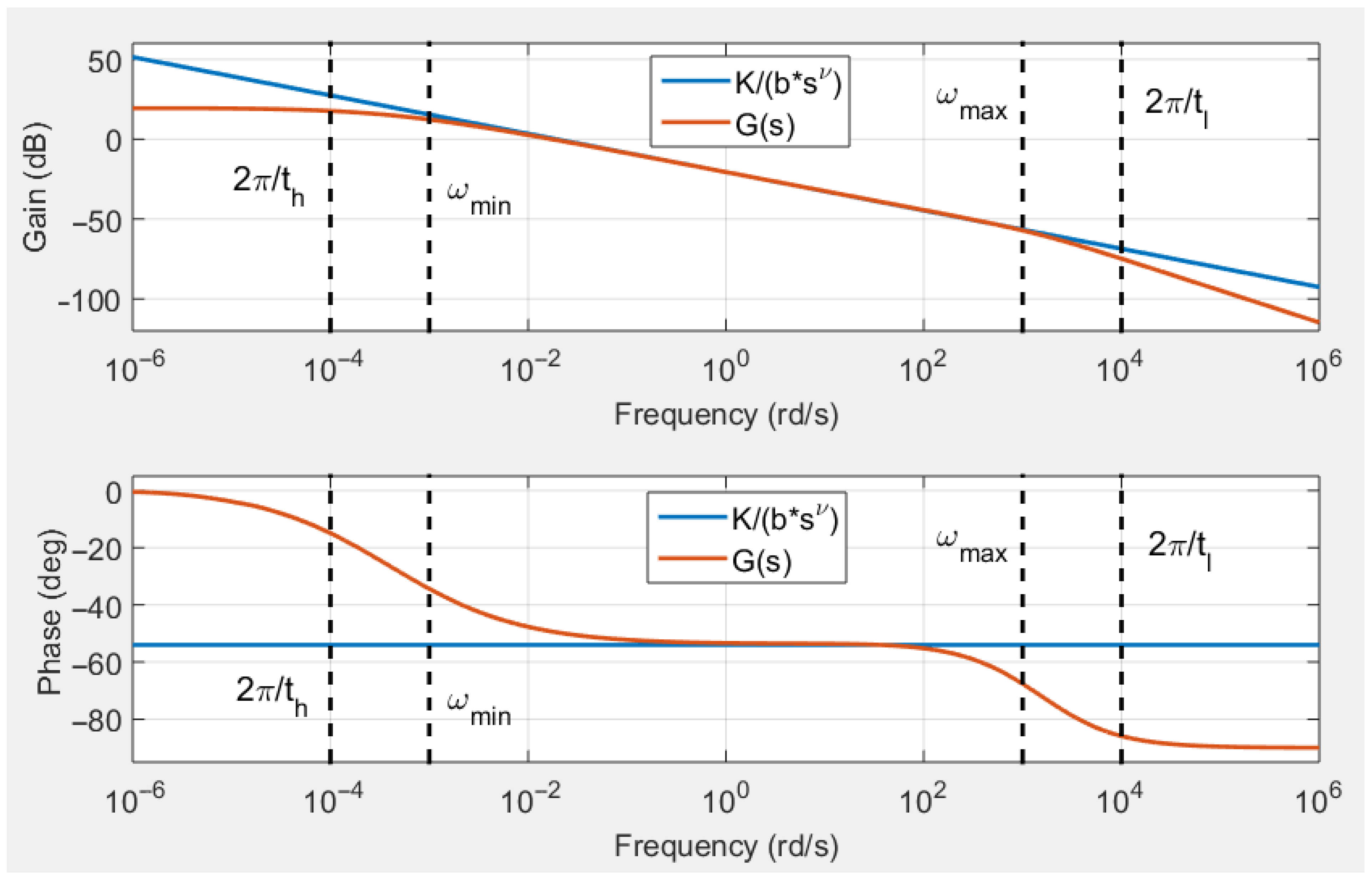
4.1. A Preliminary Analysis

Before considering a distributed time delay model, the following transfer function is analyzed

$$H\left(s\right)={\displaystyle \frac{K}{as+b{s}^{\nu }+1}},K\in ℝ$$

(25)

with $0<\nu <1$. It is assumed moreover that $0<a<b$, $a\in ℝ$, and $b\in ℝ$. The frequency response of this transfer function is:

$$H\left(j\omega \right)={\displaystyle \frac{K}{aj\omega +b{\left(j\omega \right)}^{\nu }+1}}={\displaystyle \frac{K}{aj\omega +b{\omega }^{\nu }\left(cos\left(\nu \frac{\pi }{2}\right)+jsin\left(\nu \frac{\pi }{2}\right)\right)+1}}$$

(26)

The phase and gain of $H\left(j\omega \right)$ are given by:

$$\phi \left(H\left(j\omega \right)\right)=-atan\left({\displaystyle \frac{a\omega +b{\omega }^{\nu }sin\left(\nu \frac{\pi }{2}\right)}{1+b{\omega }^{\nu }cos\left(\nu \frac{\pi }{2}\right)}}\right)$$

(27)

and

$$\left|H\left(j\omega \right)\right|={\displaystyle \frac{K}{\sqrt{2b{\omega }^{\nu +1}asin\left(\nu \frac{\pi }{2}\right)+2b{\omega }^{\nu }cos\left(\nu \frac{\pi }{2}\right)+{\omega }^{2\nu }{b}^2+{\omega }^2{a}^2+1}}}$$

(28)

These relations highlight that:

-

for $\omega \to 0$, $\phi \left(H\left(j\omega \right)\right)\to 0$;

-

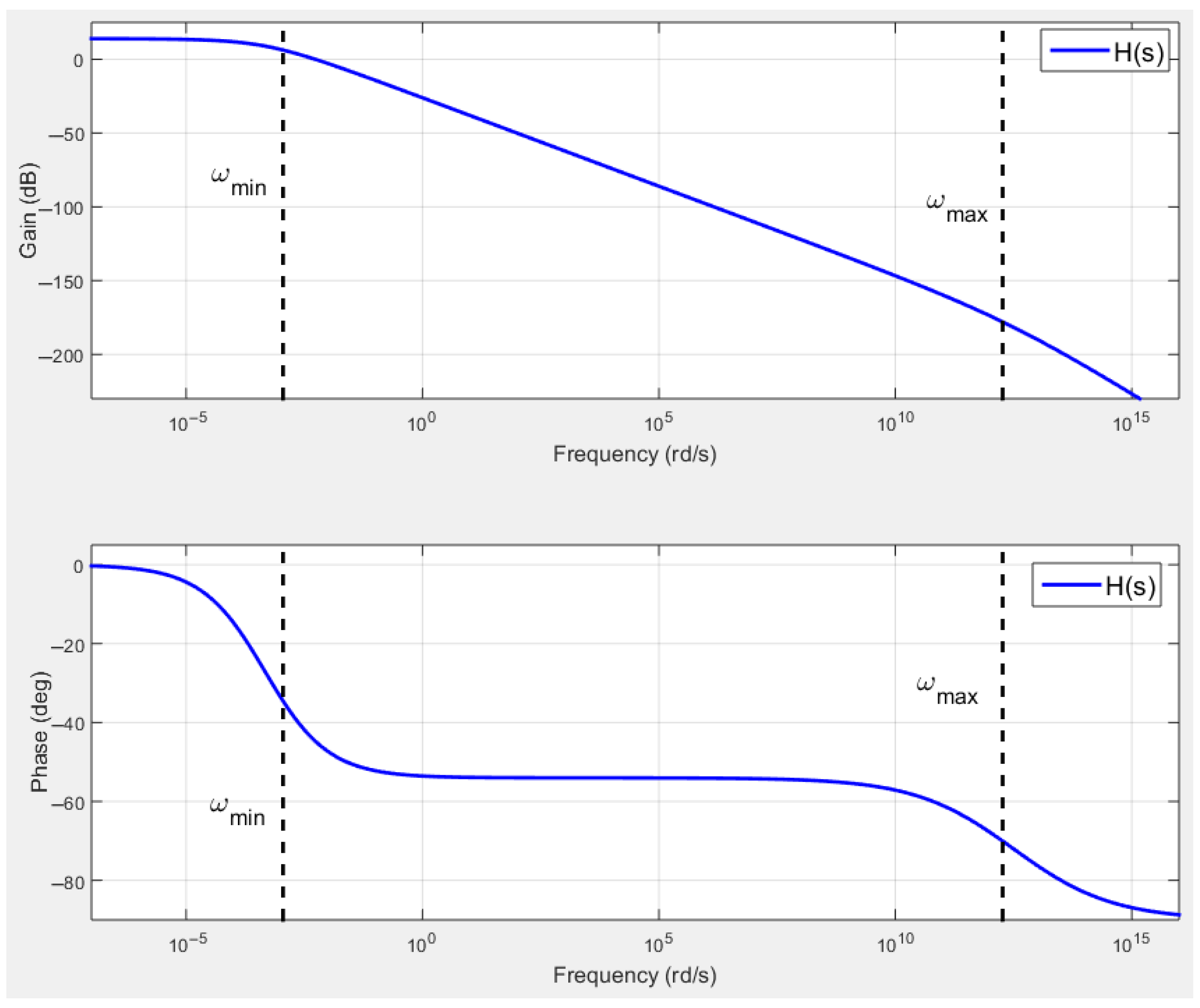
for frequencies such as $1<b{\omega }^{\nu }cos\left(\nu {\displaystyle \frac{\pi }{2}}\right)$ and $a\omega <b{\omega }^{\nu }sin\left(\nu {\displaystyle \frac{\pi }{2}}\right)$, then

$$\phi \left(H\left(j\omega \right)\right)\approx -atan\left({\displaystyle \frac{b{\omega }^{\nu }sin\left(\nu \frac{\pi }{2}\right)}{b{\omega }^{\nu }cos\left(\nu \frac{\pi }{2}\right)}}\right)=-\nu {\displaystyle \frac{\pi }{2}}$$

(29)

$$\left|H\left(j\omega \right)\right|\approx {\displaystyle \frac{K}{{\omega }^{\nu }b}}$$

(30)

for $\omega \to +\infty , \phi \left(H\left(j\omega \right)\right)\approx -atan\left({\displaystyle \frac{a\omega }{b{\omega }^{\nu }cos\left(\nu \frac{\pi }{2}\right)}}\right)=-{\displaystyle \frac{\pi }{2}}$.

Clearly, the transfer function $H\left(s\right)$ exhibits a fractional behavior within the frequency band defined by:

$$1〈b{\omega }^{\nu }cos\left(\nu {\displaystyle \frac{\pi }{2}}\right) \mathrm{thus} \omega 〉 {\displaystyle \frac{1}{{\left(bcos\left(\nu \frac{\pi }{2}\right)\right)}^{\frac{1}{\nu }}}}={\omega }_{min}$$

(31)

and

$$a\omega <b{\omega }^{\nu }sin\left(\nu {\displaystyle \frac{\pi }{2}}\right) \mathrm{thus} \omega <{\left({\displaystyle \frac{bsin\left(\nu \frac{\pi }{2}\right)}{a}}\right)}^{{\displaystyle \frac{1}{1-\nu }}}={\omega }_{max}.$$

(32)

Conversely, it is possible to generate fractional behavior on the interval $\left[{\omega }_{min},{\omega }_{max}\right]$ with the transfer function $H\left(s\right)$ if

$$b={\displaystyle \frac{1}{{{\omega }_{min}}^{\nu }cos\left(\nu \frac{\pi }{2}\right)}} \mathrm{and} a={\displaystyle \frac{tan\left(\nu \frac{\pi }{2}\right)}{{{\omega }_{min}}^{\nu }{{\omega }_{max}}^{1-\nu }}}$$

(33)

as shown by Figure 3, obtained with $a=0.001$, $b=100$, $K=5$, and $\nu =0.6$.

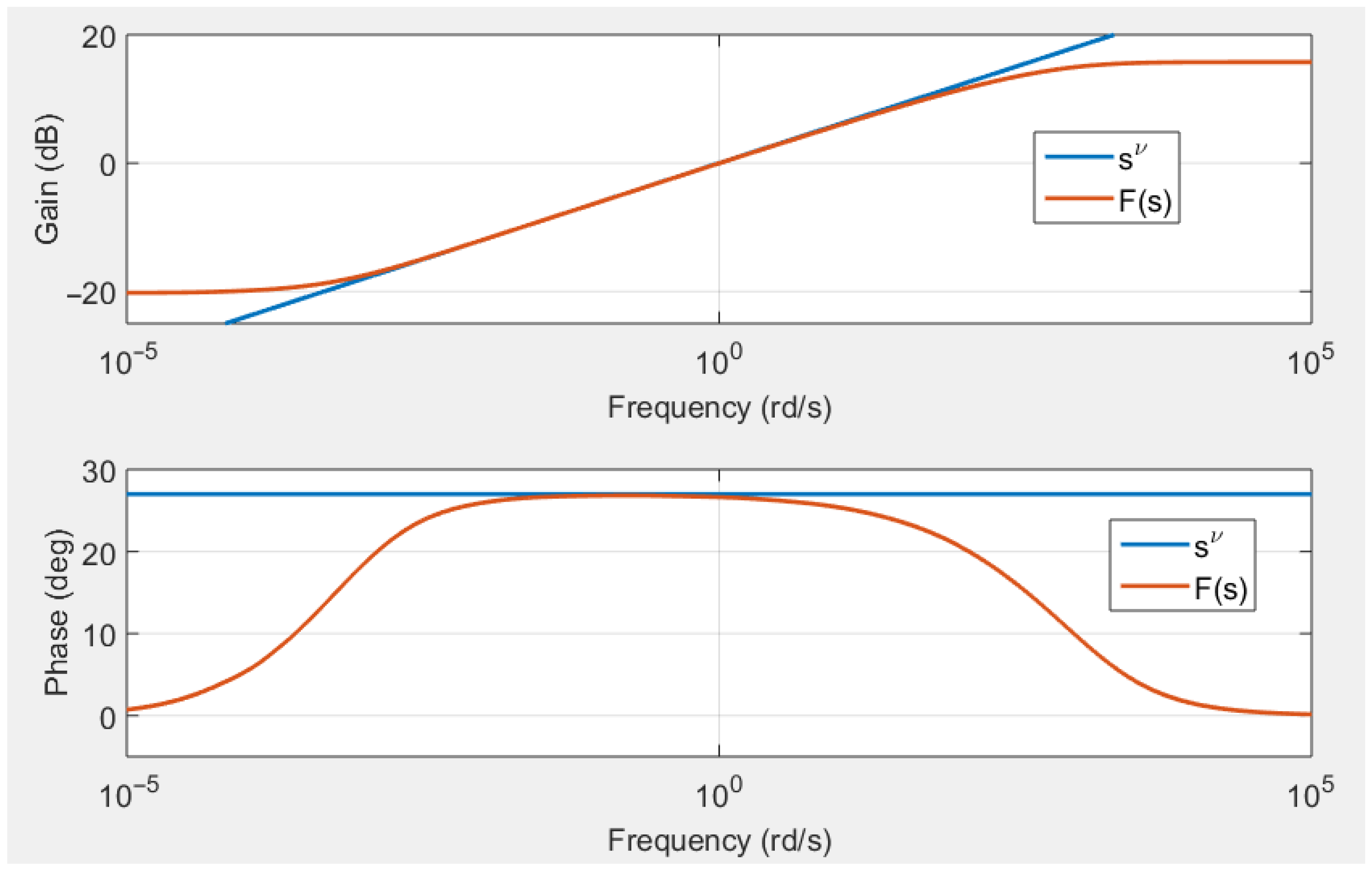
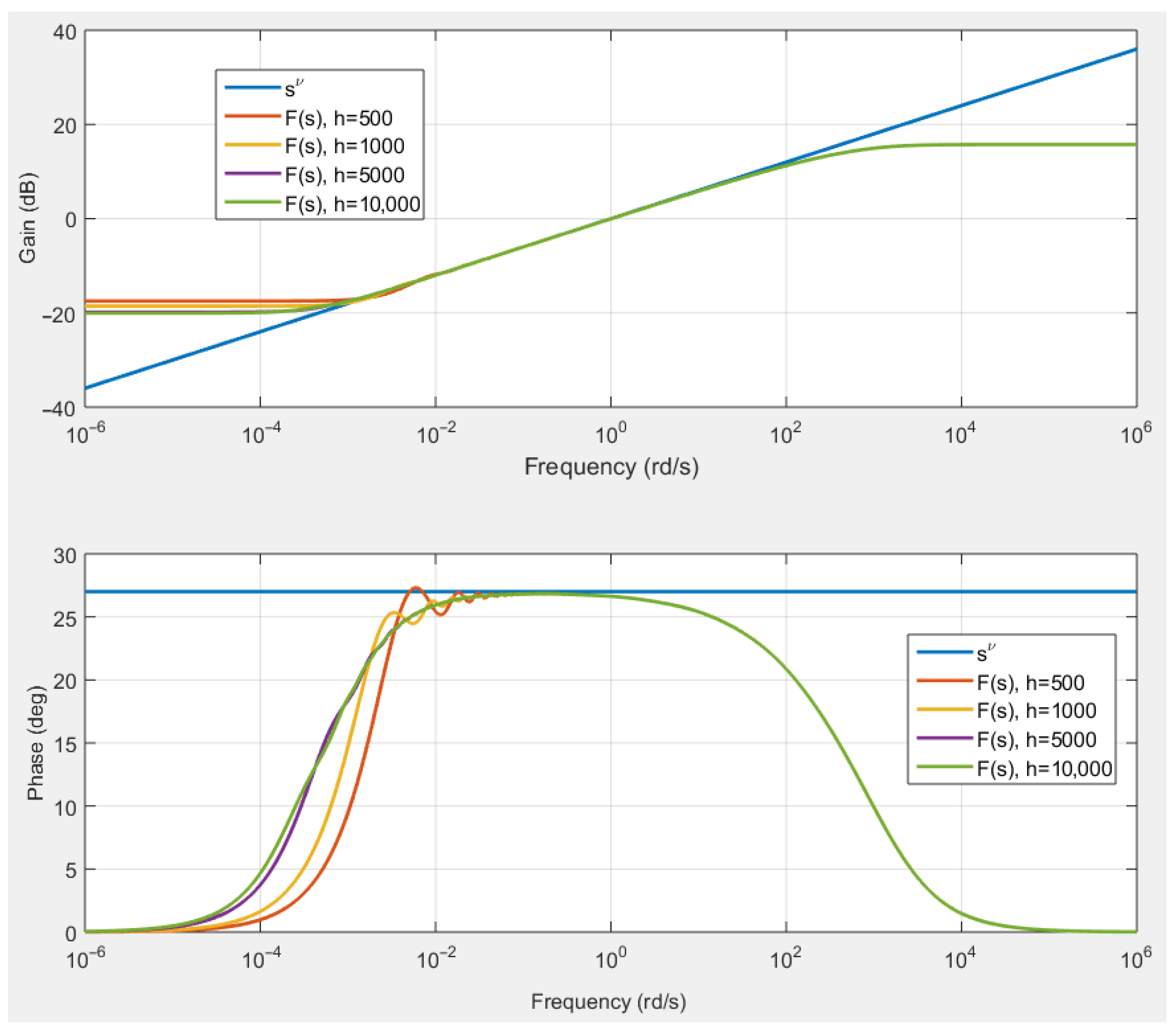
4.2. Order ν Fractional Derivative-like Behavior

According to relation (1), the fractional integral of $z\left(t\right)$ is given by the convolution integral of $z\left(t\right)$

$${\mathit{I}}_0^{\nu }\left[z\left(t\right)\right]={{\displaystyle \int }}_0^t\eta \left(t-\tau \right)z\left(\tau \right)d\tau ,$$

(34)

with the kernel

$$\eta \left(t\right)={\displaystyle \frac{t^{\nu -1}}{\mathit{\Gamma }\left(\nu \right)}}$$

(35)

The kernel $\eta \left(t\right)$ in (35) is singular. This poses several problems detailed in [36]. Moreover, operator (34) is physically inconsistent, as it exhibits infinitely small and large time constants [16].

As mentioned in [37], this singularity is not necessary to generate fractional behaviors. Many other functions can be chosen to replace kernel $\eta \left(t\right)$ in order to generate fractional integral-like behaviors over a given time/frequency band. Among this infinite set, inspiration can be drawn from [38] in which non-singular rational kernels are studied. They are defined by

$${\eta }_a\left(t\right)=C_0{\displaystyle \frac{{{\displaystyle \prod }}_{j=1}^N\left(\frac{t}{t_j^{\prime }}+1\right)}{{{\displaystyle \prod }}_{j=1}^N\left(\frac{t}{t_j}+1\right)}},t_j^{\prime }\in {ℝ}_{+}^{*}, t_j\in {ℝ}_{+}^{*}$$

(36)

and permit an approximation of the power-law function

$$t^{-\nu },\nu \in ℝ,$$

(37)

in which the pole $-t_j$, the zeros $-t_j^{\prime }$, and the gain $C_0$ are computed using the following Algorithm 1.

Algorithm 1 Functions ${\eta }_a\left(t\right)$ synthesis [38]
Choose the time interval $\left[t_l,t_h\right]$ on which the approximation is required and the degree $N$ (number of poles and zeros) of the rational function. Compute $r=\sqrt[N]{{\displaystyle \frac{t_h}{t_l}}}$ Compute $\beta =r^{\nu }$ and $\alpha ={\displaystyle \frac{r}{\beta }}$. Compute $t_1=t_l\ast \sqrt{\alpha }$ and the other $t_j^{\prime }$ and $t_j$ using relations.
$\beta ={\displaystyle \frac{t_j^{\prime }}{t_j}} \mathrm{and} \alpha ={\displaystyle \frac{t_{j+1}}{t_j^{\prime }}}$.	(38)
5. Compute $C_0={\left(t_m\right)}^{-\nu }{\displaystyle \frac{{{\displaystyle \prod }}_{j=1}^N\left(\frac{t_m}{t_j}+1\right)}{{{\displaystyle \prod }}_{j=1}^N\left(\frac{t_m}{t_j^{\prime }}+1\right)}}$ with $t_m=\sqrt{t_l{t}_h}$ (middle of $\left[t_l,t_h\right]$ on a logarithmic scale). 6. Compute the approximation ${\eta }_a\left(t\right)=C_0{\displaystyle \frac{{{\displaystyle \prod }}_{j=1}^N\left(\frac{t}{t_j^{\prime }}+1\right)}{{{\displaystyle \prod }}_{j=1}^N\left(\frac{t}{t_j}+1\right)}}$

A fractional derivative behavior over a given time/frequency band can thus be obtained using relations (2) and (34) in which kernel $\eta \left(t\right)$ is replaced by kernel ${\eta }_a\left(t\right)$:

$$D^{\nu }\left[z\left(t\right)\right]\approx {\displaystyle \frac{1}{\Gamma \left(1-\nu \right)}}{\displaystyle \frac{\mathrm{d}}{dt}}{{\displaystyle \int }}_0^t{\eta }_a\left(t-\tau \right)z\left(\tau \right)d\tau$$

(39)

and thus after computation of the derivative

$$D^{\nu }\left[z\left(t\right)\right]\approx {\displaystyle \frac{1}{\Gamma \left(1-\nu \right)}}{{\displaystyle \int }}_0^t{\displaystyle \frac{d{\eta }_a\left(\zeta \right)}{d\zeta }}\left(t-\tau \right)z\left(\tau \right)d\tau +{\displaystyle \frac{1}{\Gamma \left(1-\nu \right)}}{\eta }_a\left(0\right)z\left(t\right)$$

(40)

Using the change of variable $\xi =t-\tau$ and thus $\tau =t-\xi$ and $d\tau =-\mathrm{d}\xi$, relation (40) becomes

$$D^{\nu }\left[z\left(t\right)\right]\approx {\displaystyle \frac{1}{\Gamma \left(1-\nu \right)}}{{\displaystyle \int }}_0^t{\displaystyle \frac{d{\eta }_a\left(\zeta \right)}{d\zeta }}\left(\xi \right)z\left(t-\xi \right)d\xi +{\displaystyle \frac{C_0}{\Gamma \left(1-\nu \right)}}z\left(t\right)$$

(41)

as ${\eta }_a\left(0\right)=C_0$, which can also be approximated by

$$D^{\nu }\left[z\left(t\right)\right]\approx {\displaystyle \frac{1}{\Gamma \left(1-\nu \right)}}{{\displaystyle \int }}_0^h{\displaystyle \frac{d{\eta }_a\left(\zeta \right)}{d\zeta }}\left(\xi \right)z\left(t-\xi \right)d\xi +{\displaystyle \frac{C_0}{\Gamma \left(1-\nu \right)}}z\left(t\right)$$

(42)

in which the integral upper bound $t$ is replaced by $h\in {ℝ}^{+}$. The Laplace transform of relation (42) leads to

$$\mathcal{L}\left\{D^{\nu }\left[z\left(t\right)\right]\right\}\approx Z\left(s\right)\left({\displaystyle \frac{1}{\Gamma \left(1-\nu \right)}}{{\displaystyle \int }}_0^h{\displaystyle \frac{d{\eta }_a\left(\zeta \right)}{d\zeta }}\left(\xi \right)e^{-\xi s}d\xi +{\displaystyle \frac{C_0}{\Gamma \left(1-\nu \right)}}\right)$$

(43)

with $Z\left(s\right)=\mathcal{L}\left\{z\left(t\right)\right\}$. The function

$$F\left(s\right)={\displaystyle \frac{1}{\Gamma \left(1-\nu \right)}}{{\displaystyle \int }}_0^h{\displaystyle \frac{d{\eta }_a\left(\zeta \right)}{d\zeta }}\left(\xi \right)e^{-\xi s}d\xi +{\displaystyle \frac{C_0}{\Gamma \left(1-\nu \right)}}$$

(44)

can thus be viewed as an approximation in the Laplace domain of the transfer function $s^{\nu }$ over a frequency band. To compute the integral in (44), a partial fraction expansion of ${\eta }_a\left(\zeta \right)$ is used:

$${\eta }_a\left(\zeta \right)=C_0{\displaystyle \frac{{{\displaystyle \prod }}_{j=1}^N\left(\frac{\zeta }{t_j^{\prime }}+1\right)}{{{\displaystyle \prod }}_{j=1}^N\left(\frac{\zeta }{t_j}+1\right)}}=C_0+{\displaystyle \sum }_{j=1}^N{\displaystyle \frac{C_j}{\left(\frac{\zeta }{t_j}+1\right)}}$$

(45)

and its derivative is thus

$${\displaystyle \frac{d{\eta }_a\left(\zeta \right)}{d\zeta }}=-{\displaystyle \sum }_{j=1}^N{\displaystyle \frac{C_j}{t_j{\left(\frac{\zeta }{t_j}+1\right)}^2}}$$

(46)

$$\mathrm{As} {{\displaystyle \int }}_0^h{\displaystyle \frac{C_j}{t_j{\left(\frac{\zeta }{t_j}+1\right)}^2}}{e}^{-\xi s}d\xi C_j{\displaystyle \frac{t_j{e}^{-sh}-s{t}_j{e}^{-s{t}_j}\left(h+t_j\right)E_i\left(s\left(h+t_j\right)\right)+\left(h+t_j\right)\left(e^{s{t}_j}{E}_i\left(s{t}_j\right)s{t}_j-1\right)}{h+t_j}}$$

(47)

then

$$F\left(s\right)={\displaystyle \frac{C_0}{\Gamma \left(1-\nu \right)}}+{\displaystyle \sum }_{j=1}^N{C}_j{\displaystyle \frac{t_j{e}^{-sh}-s{t}_j{e}^{-s{t}_j}\left(h+t_j\right)E_i\left(s\left(h+t_j\right)\right)+\left(h+t_j\right)\left(e^{s{t}_j}{E}_i\left(s{t}_j\right)s{t}_j-1\right)}{\Gamma \left(1-\nu \right)\left(h+t_j\right)}}$$

(48)

where according to [39,40], the exponential integral function $E{i}_1\left(\mu \right)$ is defined by:

$$E{i}_1\left(\varsigma \right)=\underset{\mu }{\overset{\infty }{{\displaystyle \int }}}{\displaystyle \frac{e^{-x}}{x}}dx \mathrm{with} \left|arg\left(\mu \right)\right|<\pi .$$

(49)

The frequency response of the transfer function $F\left(s\right)$ given by relation (48) is represented by Figure 4 for $\nu =0.3$, $t_l={10}^{-3}$, $t_h={10}^3$, $N=7$, and $h=5000$. It is compared to the frequency response of the transfer function $s^{\nu }$. This figure clearly highlights that $F\left(s\right)$ exhibits an order $\nu$ fractional derivative behavior between the frequencies ${\omega }_l=1/t_h$ and ${\omega }_h=1/t_l$. Figure 5 evaluates the impact of parameter $h$. For several values of $h$, the gain and phase of the transfer function $F\left(s\right)$ are represented. This figure gives the following rule to avoid gain and phase ripples: $h>5t_h$.

4.3. Distributed Time Delay Models with Fractional Behaviors

Let us now consider the distributed time delay model defined by [41]

$${\displaystyle \frac{d}{dt}}x\left(t\right)=E_{0}x\left(t\right)+A_1{{\displaystyle \int }}_{-h}^{0}g\left(\theta \right)x\left(t+\theta \right)d\theta +Bu\left(t\right)$$

(50)

where $E_0\in {ℝ}^{+}$, $A_1\in {ℝ}^{+}$, and $B\in ℝ$. Using the change of variable $\theta =-\tau$ and thus $d\theta =-d\tau$, relation (50) becomes

$${\displaystyle \frac{d}{dt}}x\left(t\right)=E_{0}x\left(t\right)+A_1{{\displaystyle \int }}_0^{h}g\left(-\tau \right)x\left(t-\tau \right)d\tau +Bu\left(t\right)$$

(51)

That can be rewritten as:

$$\begin{gathered} {\displaystyle \frac{d}{dt}}x\left(t\right)=\left(E_0-{\displaystyle \frac{A_1{C}_0}{\Gamma \left(1-\nu \right)}}\right)x\left(t\right)+A_1\left({{\displaystyle \int }}_0^{h}g\left(-\tau \right)x\left(t-\tau \right)d\tau +{\displaystyle \frac{C_0}{\Gamma \left(1-\nu \right)}}x\left(t\right)\right) \\ \hspace{1em}\hspace{1em}\hspace{1em}+Bu\left(t\right)\hspace{1em}\hspace{1em}\hspace{1em}\hspace{1em}\hspace{1em}\hspace{1em}\hspace{1em}\hspace{1em}\hspace{1em}\hspace{1em}\hspace{1em}\hspace{1em}\hspace{1em}\hspace{1em}\hspace{1em}\hspace{1em}\hspace{1em} \end{gathered}$$

(52)

Using

$$A_0=\left(E_0-{\displaystyle \frac{A_1{C}_0}{\Gamma \left(1-\nu \right)}}\right),\hspace{1em}\hspace{1em}\hspace{1em}g\left(-\tau \right)={\displaystyle \frac{1}{\Gamma \left(1-\nu \right)}}{\displaystyle \frac{d{\eta }_a\left(\zeta \right)}{d\zeta }}\left(\tau \right)$$

(53)

relation (52) becomes

$${\displaystyle \frac{d}{dt}}x\left(t\right)=A_{0}x\left(t\right)+{\displaystyle \frac{A_1}{\Gamma \left(1-\nu \right)}}\left({{\displaystyle \int }}_0^h{\displaystyle \frac{d{\eta }_a\left(\zeta \right)}{d\zeta }}\left(\tau \right)x\left(t-\tau \right)d\tau +C_{0}x\left(t\right)\right)+Bu\left(t\right)$$

(54)

The Laplace transform applied to relation (54) leads to

$$sX\left(s\right)=A_{0}X\left(s\right)+{\displaystyle \frac{A_1}{\Gamma \left(1-\nu \right)}}\left({{\displaystyle \int }}_0^h{\displaystyle \frac{d{\eta }_a\left(\zeta \right)}{d\zeta }}\left(\tau \right)e^{-\tau s}d\tau +C_0\right)X\left(s\right)+BU\left(s\right)$$

(55)

with $U\left(s\right)=\mathcal{L}\left\{u\left(t\right)\right\}$, and thus

$${\displaystyle \frac{X\left(s\right)}{U\left(s\right)}}={\displaystyle \frac{B}{s-A_1\left(\frac{1}{\Gamma \left(1-\nu \right)}{{\displaystyle \int }}_0^h\frac{d{\eta }_a\left(\zeta \right)}{d\zeta }\left(\tau \right)e^{-\tau s}d\tau +\frac{C_0}{\Gamma \left(1-\nu \right)}\right)-A_0}}$$

(56)

If $a=-1/A_0, b=A_1/A_0, K=-B/A_0$, then according to Section 4.2

$${\displaystyle \frac{X\left(s\right)}{U\left(s\right)}}\approx {\displaystyle \frac{K}{as+b{s}^{\nu }+1}}=G\left(s\right)$$

(57)

and according to Section 4.1 exhibits a fractional behavior on the frequency range $\left[{\omega }_{min},{\omega }_{max}\right]$ if

$${\omega }_{min}={\displaystyle \frac{1}{{\left(bcos\left(\frac{\nu \pi }{2}\right)\right)}^{\frac{1}{\nu }}}} \mathrm{and} {\omega }_{max}=e^{-{\displaystyle \frac{ln\left(\frac{bsin\left(\frac{\nu \pi }{2}\right)}{a}\right)}{\nu -1}}}$$

(58)

provided that

$$t_h\gg {\displaystyle \frac{2\pi }{{\omega }_{min}}} \mathrm{and} t_l\ll {\displaystyle \frac{2\pi }{{\omega }_{max}}}.$$

(59)

Figure 6 shows the gain and phase diagram of the transfer function $G\left(s\right)$ (relations (57) and (58)) with $\nu =0.6$, ${\omega }_{min}={10}^{-3}rd/s$, ${\omega }_{max}={10}^3 rd/s$, and thus according to relation (33) $a=5.48$, $b=107.34$, $K=10$, $N=12$, and according to relation (60) $t_l=6.28\times {10}^{-4} s$, $t_h=6.28\times {10}^4 s$, and $h=5t_h$. A Bode diagram of the transfer function $G\left(s\right)$ is compared in Figure 6 to the Bode diagram of the fractional integrator $K/\left(b{s}^{\nu }\right)$. This figure clearly shows that a fractional behavior can be generated with distributed time delay models.

5. Physical Interpretations and Numerical Example

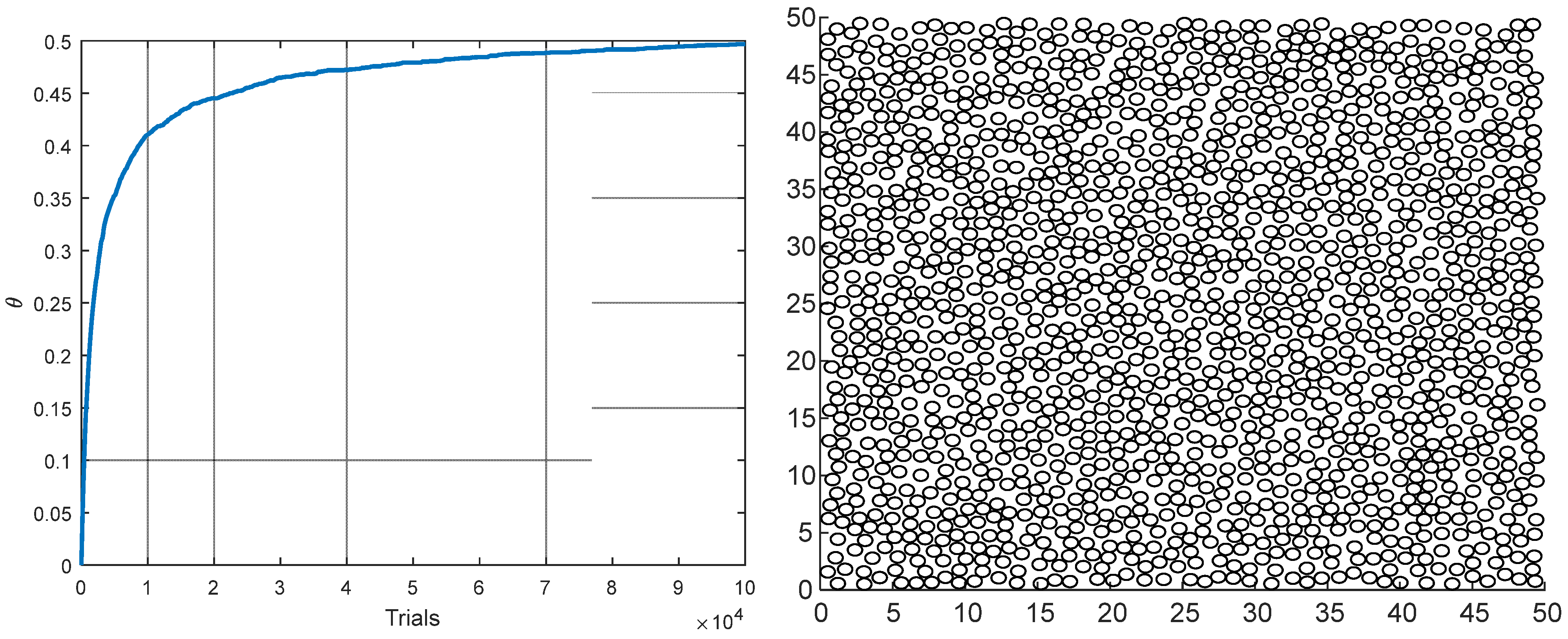
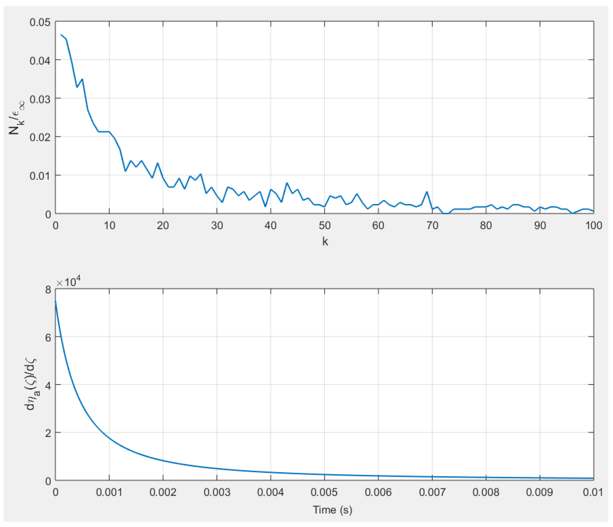
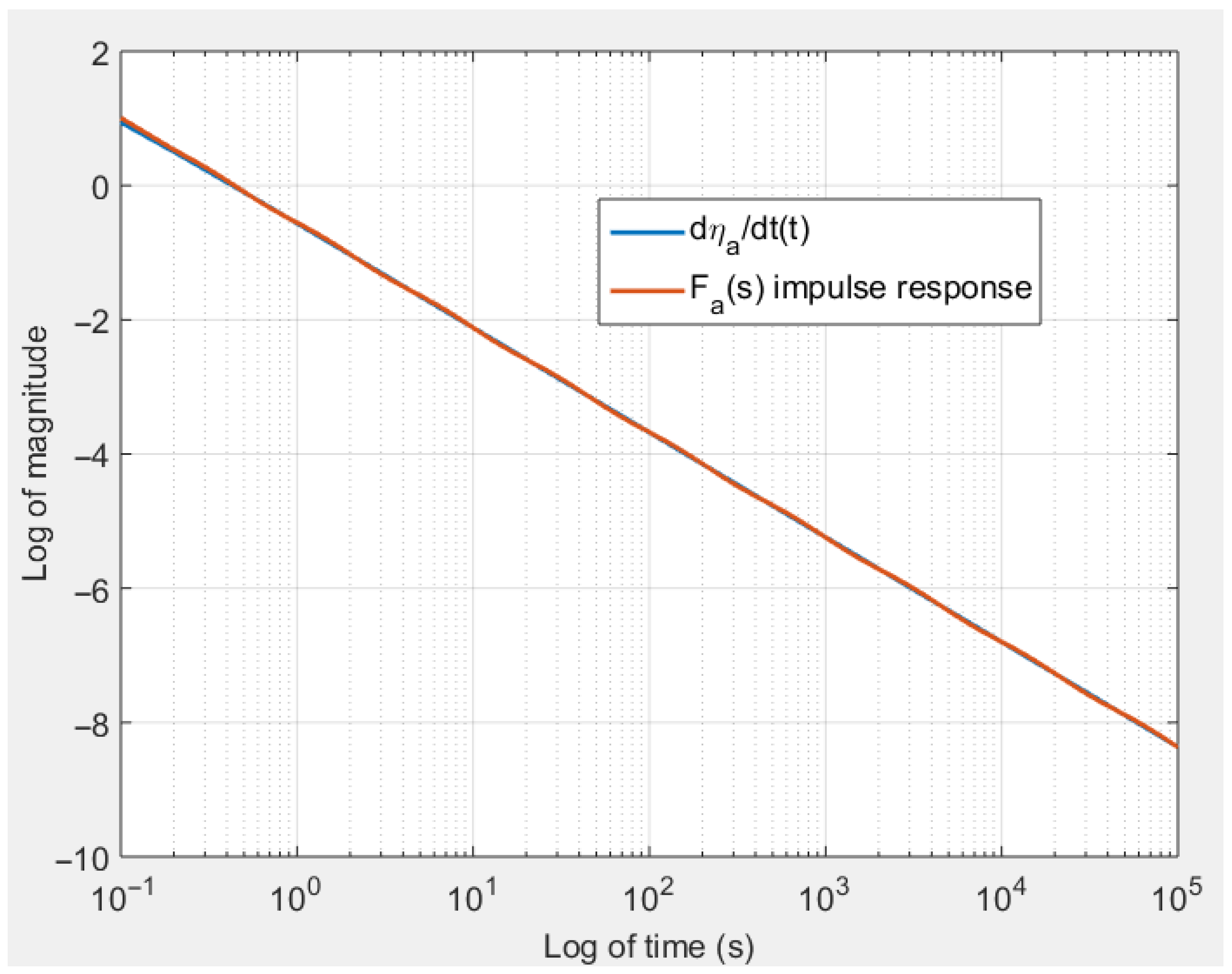
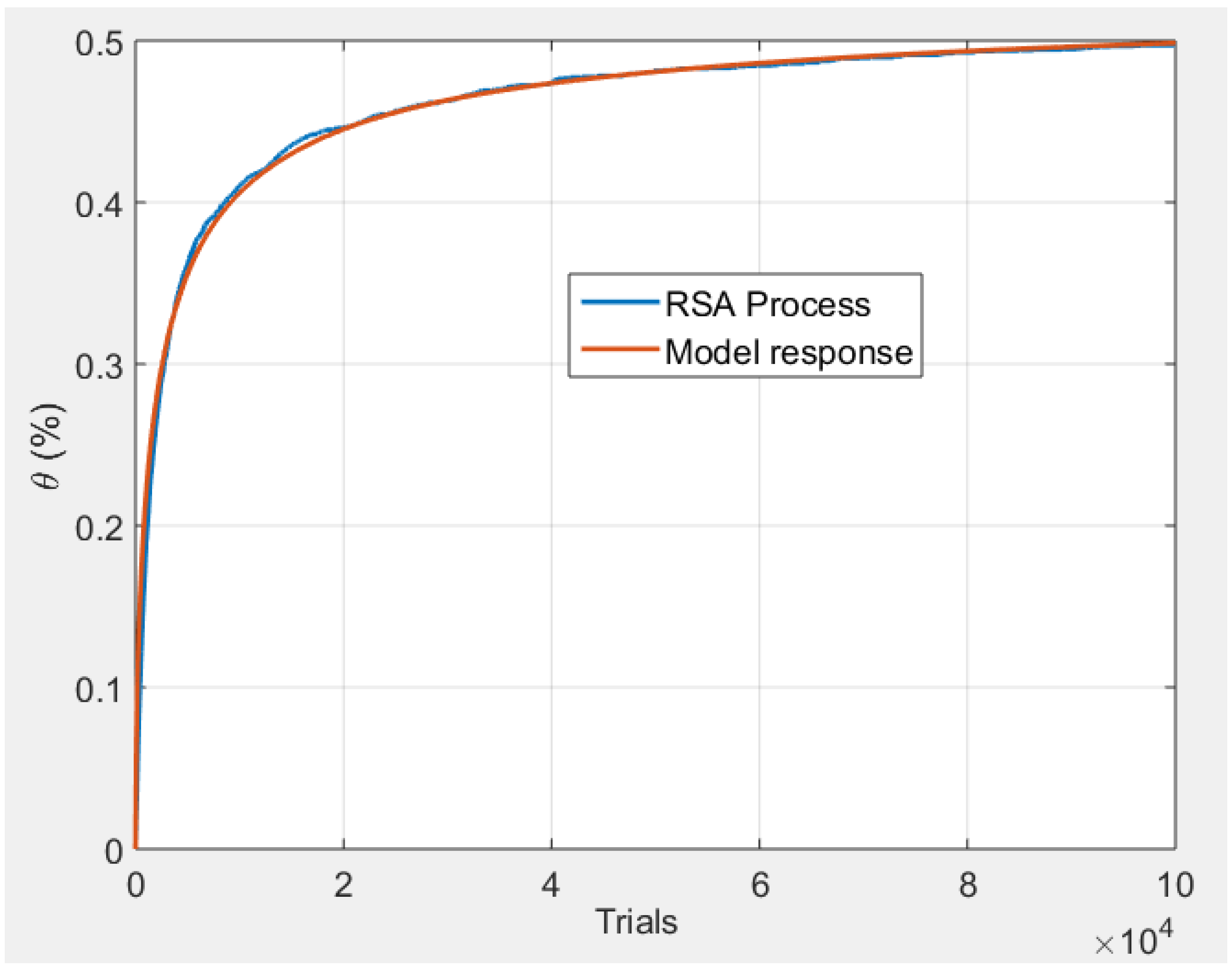
5.1. Case of Adsorption

The phenomena of adsorption and Random Sequential Adsorption (RSA) are currently utilized to demonstrate that distributed time delay models can effectively capture the dynamics of systems exhibiting fractional behaviors (see Section 4) and also represent the underlying physics that gives rise to these behaviors.

Adsorption is defined as the accumulation of a substance at the interface between two different phases [42], such as gas–liquid, gas–solid, liquid–liquid, liquid–solid, or solid–solid. This phenomenon is due to intermolecular attractive forces, which account for the cohesion observed in condensed phases, whether they are liquid or solid. Random Sequential Adsorption (RSA) [43] is a theoretical stochastic process commonly cited in the literature for the analysis of chemical adsorption. The RSA process, in conjunction with adsorption, arises from the stochastic behavior of various agents, including molecules, atoms, or individuals, within a confined geometry, such as that restricted by the presence of agents already on the surface. As indicated in the literature [44], both adsorption and RSA processes demonstrate fractional behavior.

The RSA process occurs in a sequential manner. To exemplify this, let us examine a square plane substrate with an edge length of $L$, which results in a surface area of $L^2$. It is assumed that disk-shaped particles are attracted to this substrate, with the radius $R$ of the disks being considerably smaller than the substrate size ($R\ll L$). Throughout the RSA process, particles are deposited onto the substrate one at a time. In each iteration (trial) of the process, the deposition location on the substrate is randomly determined, adhering to a uniform distribution. A particle that lands on the substrate will only adhere if it occupies an unoccupied area; otherwise, the adsorption attempt fails. Initially, at time $t_0$, the substrate’s surface is considered unoccupied.

The previously described algorithm is now utilized to generate data concerning disk particles with a radius of $R=0.5$, arranged on a square with an edge length of $L=50$. The resulting surface coverage, represented as $\theta \left(t\right)$, is shown in Figure 7 as a function of the number of trials. Furthermore, this figure also illustrates the configuration of the disks upon completion of the process.

The signal $\theta \left(t\right)$ can be estimated using a delay distribution. By analyzing the response $\theta \left(t\right)$, it is possible to ascertain the number of disks $N_k$ that adhere to the substrate during the specified time interval $\left[\left(k-1\right)T_0,k{T}_0\right]$, where $k$ belongs to ${\mathbb{N}}^{*}$. The computed values are normalized by ${ϵ}_{\infty }$, which denotes the value of $\theta \left(t\right)$ as $t$ approaches infinity, approximately equal to 0.547 as referenced in [44]. The resulting ratios $N_k/{ϵ}_{\infty }$ are then depicted in Figure 8 as a function of $k$ for $k$ within the interval [1,100].

It is important to observe that the graph of $N_k/{ϵ}_{\infty }$ depicted in Figure 8 resembles the graph of the function $d{\eta }_a\left(\zeta \right)/d\zeta$, which characterizes the delay distribution as outlined in relation (51), and is also illustrated in Figure 8.

As a result, the analysis regarding delay distribution (see [35] for a comprehensive explanation) holds a physical significance: the likelihood of encountering a time delay lasting $k{T}_0$ in the fractional behavior generated by the RSA process corresponds to the probability that $N_k/{\epsilon }_{\infty }$ disks occupy a position within the time frame $\left[\left(k-1\right)T_0,k{T}_0\right]$.

Consequently, the interpretation in terms of delay distribution (see [35] for a more detailed demonstration) has a physical meaning: the probability to find a time delay with duration $k{T}_0$ in the fractional behavior produced by the RSA process is also the probability that $N_k/{ϵ}_{\infty }$ disks find a place in the time interval $\left[\left(k-1\right)T_0,k{T}_0\right]$.

Mathematical and physical considerations are proposed in [45,46] to show the link of adsorption phenomenon with delay-based models. In order to illustrate even better the interest of distributed delay models to model RSA (and thus adsorption) phenomena and fractional behaviors, it is now proposed to use relation (54) to fit the kinetic shown by Figure 7. In this numerical application, parameters $A_0$, $A_1$, $B$, and $\mathrm{\nu }$ of model (54) are computed using a nonlinear Levenberg–Marquardt optimization algorithm that minimizes a quadratic criterion involving the error between the model output and the response $\theta \left(t\right)$. For the implementation of model (54), the Laplace transform of ${\displaystyle \frac{d{\eta }_a\left(t\right)}{dt}}$ is approximated by a transfer function denoted $F_a\left(s\right)$, and the integral ${{\displaystyle \int }}_0^h{\displaystyle \frac{d{\eta }_a\left(\zeta \right)}{d\zeta }}\left(\tau \right)x\left(t-\tau \right)d\tau$ is treated as a convolution product. Model (55) can thus be implemented in Matlab Simulink software as shown by Figure 9. Note that the function ${\displaystyle \frac{d{\eta }_a\left(t\right)}{dt}}$ can also be implemented using a FIR model but the simulations become time consuming. In future work, the author intends to develop more specific implementation solutions based on the discretization of the integral ${{\displaystyle \int }}_0^h{\displaystyle \frac{d{\eta }_a\left(\zeta \right)}{d\zeta }}\left(\tau \right)x\left(t-\tau \right)d\tau$ after a specific change in variable that contracts the time scale.

For the definition using Algorithm 1 of the function ${\eta }_a\left(\zeta \right)$ given by relation (36), the following parameters have been used

$$t_l=0.01\mathrm{s} t_h=8\times {10}^6, N=15$$

(60)

in order to well cover the time domain on which the RSA process is studied. Transfer function $F_a\left(s\right)$ is computed using an optimization problem aiming at minimizing the error between the logarithm of the impulse response of $F_a\left(s\right)$ and ${\displaystyle \frac{d{\eta }_a\left(t\right)}{dt}}$. As the resulting transfer function is of order 16 over 16, its coefficients are not given, but Figure 10 shows a comparison using a logarithmic scale on both the abscissa and ordinate and reveals a very good approximation.

After optimization, the following values have been obtained for the parameters of model (55), the input $u\left(t\right)$ being considered as a step input of magnitude 1:

$$A_0=-0.0123A_1=-1.066\nu =0.56B=0.00659 \mathrm{and} C_0=13.40.$$

(61)

With the parameters obtained, Figure 11 compares the signal $\theta \left(t\right)$ resulting from the RSA process and the response of the distributed delay model (54). This figure highlights that model (54) fits very well, and the signal $\theta \left(t\right)$ is therefore fully capable of capturing fractional behaviors.

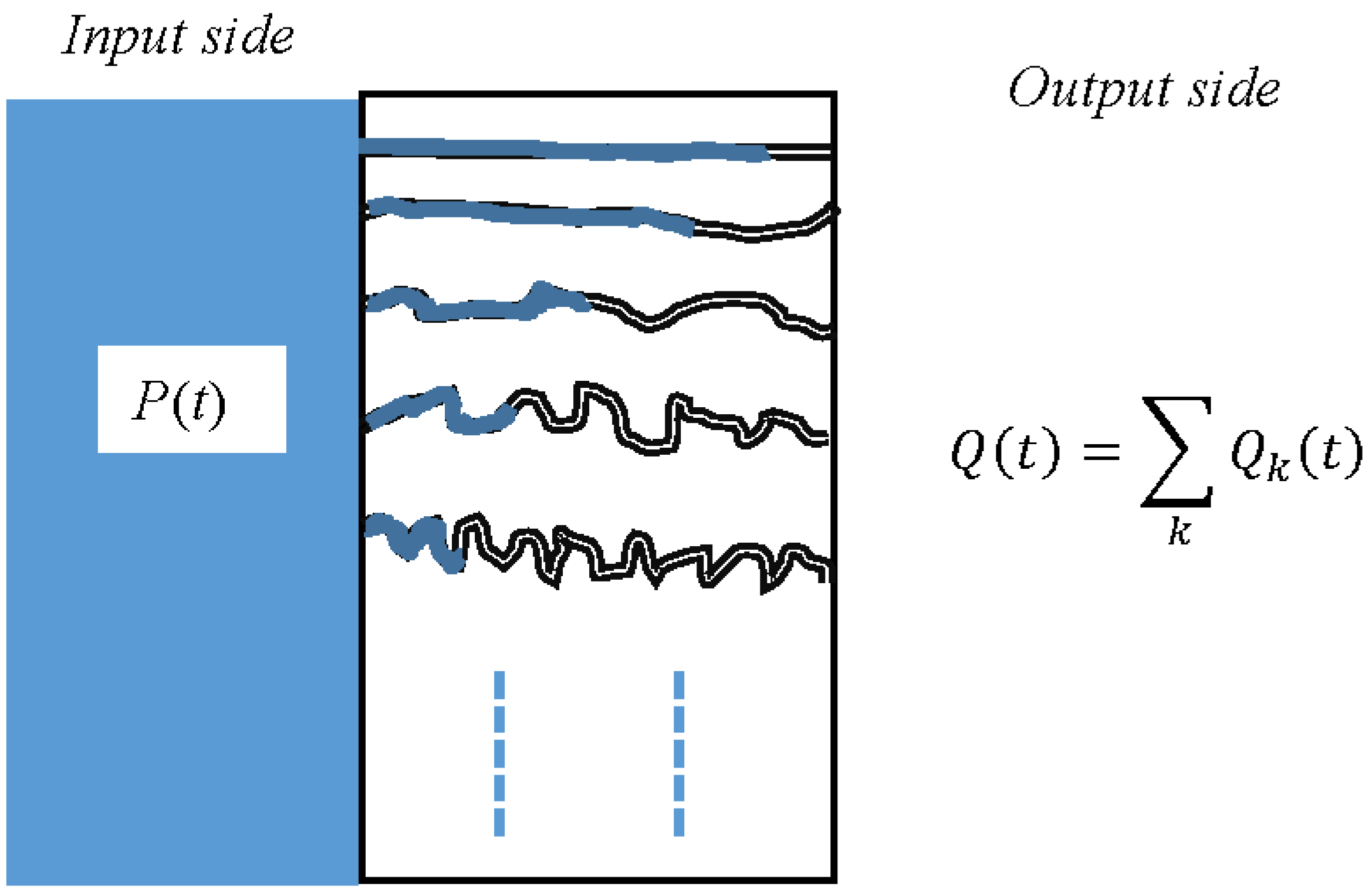
5.2. Case of Diffusion

It is widely recognized that diffusion can be accurately characterized by the concept of particle random walk [33]. Furthermore, diffusion is known to exhibit fractional behaviors of order ½ or other values in intricate environments such as fractal media [34]. Additionally, an interpretation grounded in delay distribution is feasible.

This interpretation is illustrated in Figure 12. It is assumed that the medium consists of channels of differing lengths. Prior to the introduction of water into the medium, these channels are considered to be devoid of fluid. When the fluid pressure $P\left(t\right)$ is applied at the input side, it generates a flow within the channels, resulting in a total output flow denoted as $Q\left(t\right)$, which is the aggregate of the flow generated by each individual channel, represented as $Q_k\left(t\right)$:

$$Q\left(t\right)={\displaystyle \sum }_k{Q}_k\left(t\right)$$

(62)

The flow $Q_k\left(t\right)$ is influenced by the pressure $P\left(t\right)$ and the reciprocal of the hydraulic resistance $R_k$ for each channel. Additionally, because of variations in channel length, each flow $Q_k\left(t\right)$ arrives at the output side with a time delay $T_k$ that is contingent upon the channel length, resulting in the following relationship for each $Q_k\left(t\right)$:

$$Q_k\left(t\right)={\displaystyle \frac{1}{R_k}}P\left(t-T_k\right)$$

(63)

Thus, for relation (61):

$$Q\left(t\right)={\displaystyle \sum }_k{\displaystyle \frac{1}{R_k}}P\left(t-T_k\right)$$

(64)

If $Q_{\infty }$ represents the steady-state value of the flow $Q\left(t\right)$ when $P\left(t\right)$ is a unit step, then this modeling approach allows us to interpret the coefficients $1/\left(Q_{\infty }{R}_k\right)$ as the likelihood of experiencing a delay of duration $T_k$ in the fractional behavior resulting from diffusion phenomena. More concretely, $1/\left(Q_{\infty }{R}_k\right)$ can be associated with a distribution of channel lengths and the probability of locating the relevant channel within the analyzed system.

The link of diffusion process with delay distribution can also be demonstrated analytically. Let us consider the problem

$${\displaystyle \frac{\partial v\left(x,t\right)}{\partial x}}=D{\displaystyle \frac{{\partial }^{2}v\left(x,t\right)}{\partial x^2}} \mathrm{with} v\left(x,0\right)=0 \mathrm{and} v\left(0,t\right)=u\left(t\right).$$

(65)

The solution to this problem is given by

$$u\left(x,t\right)={{\displaystyle \int }}_0^{t}G\left(x,\tau \right)u\left(t-\tau \right)d\tau$$

(66)

with

$$G\left(x,t\right)={\displaystyle \frac{x}{2\sqrt{\pi D{t}^3}}}{e}^{\left(-{\displaystyle \frac{x^2}{4Dt}}\right)}$$

(67)

The causal kernel $G\left(x,t\right)$ can thus be viewed as a probability density that explicitly describes the distribution of times of passage at position $x$ for an impulse applied at $x=0$.

6. Conclusions

This study illustrates that distributed time delay models can exhibit fractional behaviors under some conditions, among various other classes of behaviors. They thus can be used to model fractional behaviors using adapted methods which remain to be developed. Given the prevalence of various real-world phenomena that display fractional behaviors, including those that create fractals or function within fractal geometries, it is crucial to develop models capable of accurately representing these phenomena. This necessity is heightened by the fact that the fractional models commonly referenced in the existing literature have revealed certain limitations and inconsistencies in their physical applications. Consequently, this paper proposes discretely and continuously distributed time varying models to capture fractional behaviors. In the continuous time case, it employs a non-singular rational kernel with interlaced poles and zeros within the integral term of the state space representation of a distributed time delay model to effectively generate fractional behavior. Ultimately, the findings indicate that utilizing distributed delays to represent systems characterized by fractional behaviors is physically justifiable. In numerous instances, fractional behaviors arise from the sequential actions of multiple agents operating within a constrained environment, all striving to achieve the same goal within varying timeframes.

The author aims to further validate the efficacy of distributed time delay models in capturing fractional behavior by expanding the previously obtained results to encompass multi-state and multivariable models by considering diagonal structures of the form

$$\begin{array}{c}{\displaystyle \frac{d}{dt}}\left[\begin{array}{c}{x}_1\left(t\right)\\ ⋮\\ x_n\left(t\right)\end{array}\right]=+\left[\begin{array}{c}{E}_0^1{x}_1\left(t\right)+A_1^1{{\displaystyle \int }}_{-h}^0{g}_1\left(\theta \right)x_1\left(t+\theta \right)d\theta \\ ⋮\\ E_0^n{x}_n\left(t\right)+A_1^1{{\displaystyle \int }}_{-h}^0{g}_n\left(\theta \right)x_n\left(t+\theta \right)d\theta \end{array}\right]+Bu\left(t\right)\\ z\left(t\right)=C\left[\begin{array}{c}{x}_1\left(t\right)\\ ⋮\\ x_n\left(t\right)\end{array}\right]\end{array} \begin{array}{c}B\in {ℝ}^{n\mathrm{x}m}\\ C\in {ℝ}^{p\mathrm{x}n}\end{array}$$

for the continuous time case and

$$\begin{array}{c}\left[\begin{array}{c}{x}_1\left(k+1\right)\\ ⋮\\ x_n\left(k+1\right)\end{array}\right]={\displaystyle {\displaystyle \sum }_{j=0}^{k-1}}\left[\begin{array}{c}{F}_j^1{x}_1\left(k-\mathrm{j}\right)\\ ⋮\\ F_j^n{x}_n\left(k-\mathrm{j}\right)\end{array}\right]x\left(k-j\right)+M_{1}u\left(k\right)\\ y\left(k\right)=C\left[\begin{array}{c}{x}_1\left(k+1\right)\\ ⋮\\ x_n\left(k+1\right)\end{array}\right]+M_{0}u\left(k\right)\end{array} \begin{array}{c}{M}_1\in {ℝ}^{n\mathrm{x}m}\\ C\in {ℝ}^{p\mathrm{x}n}\\ M_0\in {ℝ}^{p\mathrm{x}m}\end{array}$$

for the discrete time case.

The author wishes also to develop efficient numerical schemes for the implementation the integral ${{\displaystyle \int }}_0^h{\displaystyle \frac{d{\eta }_a\left(\zeta \right)}{d\zeta }}\left(\tau \right)x\left(t-\tau \right)d\tau$ using a specific change in variable that contracts the time scale, and to create identification methods for considered models drawing inspiration in particular from [47], and applying them to actual physical systems such as batteries.

References

- Mandelbrot, B. The Fractal Geometry of Nature, 3rd ed.; W.H. Freeman and Comp.: New York, NY, USA, 1983. [Google Scholar]
- Kopelman, R. Fractal Reaction Kinetics. Science 1988, 241, 1620–1626. [Google Scholar] [CrossRef] [PubMed]
- Sapoval, B. Universalités et Fractales: Jeux d’enfant ou délits d’initié? Editions Flammarion: Paris, France, 1997. [Google Scholar]
- Le Mehaute, A.; Crepy, G. Introduction to transfer and motion in fractal media: The geometry of kinetics. Solid State Ion. 1983, 9–10, 17–30. [Google Scholar] [CrossRef]
- Krapivsky, P.L.; Redner, S.; Ben-Naim, E. A Kinetic View of Statistical Physics; Cambridge University Press: Cambridge, UK, 2010. [Google Scholar]
- Freeborn, T.J.; Maundy, B.; Elwakil, A.S. Fractional-order models of supercapacitors, batteries and fuel cells: A survey. Mater. Renew. Sustain. Energy 2015, 4, 9. [Google Scholar] [CrossRef]
- Magin, R.L. Fractional calculus models of complex dynamics in biological tissues. Comput. Math. Appl. 2010, 59, 1586–1593. [Google Scholar] [CrossRef]
- Alhasan, A.S.H.; Saranya, S.; Al-Mdallal, Q.M. Fractional derivative modeling of heat transfer and fluid flow around a contracting permeable infinite cylinder, Computational study. Partial. Differ. Equ. Appl. Math. 2024, 11, 100794. [Google Scholar] [CrossRef]
- Hristov, J. Response functions in linear viscoelastic constitutive equations and related fractional operators. Math. Model. Nat. Phenom. 2019, 14, 305. [Google Scholar] [CrossRef]
- Monje, C.A.; Chen, Y.; Vinagre, B.M.; Xue, D.; Feliu, V. Fractional-order Systems and Controls: Fundamentals and Applications. In Advances in Industrial Control Series; Springer: London, UK, 2010. [Google Scholar]
- Samko, S.G.; Kilbas, A.A.; Marichev, O.I. Fractional Integrals and Derivatives: Theory and Applications; Gordon and Breach Science Publishers: New York, NY, USA, 1993. [Google Scholar]
- Dokoumetzidis, A.; Magin, R.; Macheras, P. A commentary on fractionalization of multi-compartmental models. Pharm. Pharm. 2010, 37, 203–207. [Google Scholar] [CrossRef]
- Balint, A.M.; Balint, S. Mathematical Description of the Groundwater Flow and that of the Impurity Spread, Which Use Temporal Caputo or Riemann-Liouville Fractional Partial Derivatives, Is Non-objective. Fractal Fract. 2020, 4, 36. [Google Scholar] [CrossRef]
- Pantokratoras, A. Comment on the paper “Fractional order model of thermo-solutal and magnetic nanoparticles transport for drug delivery applications, Subrata Maiti, Sachin Shaw, G.C. Shit, [Colloids Surf. B Biointerfaces, 203(2021) 111754]”. Colloids Surf. B Biointerfaces 2023, 222, 113074. [Google Scholar] [CrossRef]
- Mei, J. A Closer Look at Ion Transport; Nova Science Publishers: Hauppauge, NY, USA, 2025. [Google Scholar]
- Sabatier, J. Fractional Order Models Are Doubly Infinite Dimensional Models and thus of Infinite Memory: Consequences on Initialization and Some Solutions. Symmetry 2021, 13, 1099. [Google Scholar] [CrossRef]
- Trigeassou, J.C.; Maamri, N. Putting an End to the Physical Initial Conditions of the Caputo Derivative: The Infinite State Solution. Fractal Fract. 2025, 9, 252. [Google Scholar] [CrossRef]
- Caputo, M.; Fabrizio, M. A new definition of fractional derivative without singular kernel. Prog. Fract. Differ. Appl. 2015, 1, 73–85. [Google Scholar]
- Atangana, A.; Baleanu, D. New fractional derivatives with nonlocal and non-singular kernel: Theory and application to heat, transfer model. Therm. Sci. 2016, 20, 763–769. [Google Scholar] [CrossRef]
- Montseny, G. Diffusive representation of pseudo-differential time-operators. ESAIM Proc. 1998, 5, 159–175. [Google Scholar] [CrossRef]
- Matignon, D. Stability properties for generalized fractional differential systems. ESAIM Proc. 1998, 5, 145–158. [Google Scholar] [CrossRef]
- Verhulst, P.F. Recherches Mathématiques sur la loi d’accroissement de la Population; Nouveaux Mémoires de L’académie Royale Des Sciences et Belles-Lettres de Bruxelles: Washington, DC, USA, 1845; Volume 18, pp. 14–54. [Google Scholar]
- Tartaglione, V.; Sabatier, J.; Farges, C. Adsorption on Fractal Surfaces: A Non Linear Modeling Approach of a Fractional Behavior. Fractal Fract. 2021, 5, 65. [Google Scholar] [CrossRef]
- Avrami, M. Kinetics of Phase Change. I General Theory. J. Chem. Phys. 1939, 7, 1103–1112. [Google Scholar] [CrossRef]
- Fanfoni, M.; Tomellini, M. The Johnson-Mehl-Avrami-Kohnogorov Model: A Brief Review. Nuovo C. D 1998, 20, 1171–1182. [Google Scholar] [CrossRef]
- Sun, H.; Wang, Y.; Yu, L.; Yu, X. A discussion on nonlocality: From fractional derivative model to peridynamic model. Commun. Nonlinear Sci. Numer. Simul. 2022, 114, 106604. [Google Scholar] [CrossRef]
- Sabatier, J. Beyond the Particular Case of Circuits with Geometrically Distributed Components for Approximation of Fractional Order Models: Application to a New Class of Model for Power Law Type Long Memory Behaviour Modelling. J. Adv. Res. 2020, 25, 243–255. [Google Scholar] [CrossRef]
- Sabatier, J. Power Law Type Long Memory Behaviors Modeled with Distributed Time Delay Systems. Fractal Fract. 2020, 4, 1. [Google Scholar] [CrossRef]
- Capelas de Oliveira, E.; Tenreiro, M.J.A. A review of definitions for fractional derivatives and integral. Math. Probl. Eng. 2014, 2014, 1–7. [Google Scholar] [CrossRef]
- Kilbas, A.A.; Srivastava, H.M.; Trujillo, J.J. Theory and Applications of Fractional Differential Equations; Elsevier Science: Amsterdam, The Netherlands, 2006; Volume 204. [Google Scholar]
- Ortigueira, M.D.; Coito, F. From differences to derivatives. Fract. Calc. Appl. Anal. 2004, 7, 459–471. [Google Scholar]
- Oldham, K.; Spanier, J. The Fractional Calculus; Academic Press: Cambridge, MA, USA, 1974. [Google Scholar]
- Masuda, N.; Porter, M.A.; Lambiotte, R. Random walks and diffusion on networks. Phys. Rep. 2017, 716–717, 1–58. [Google Scholar] [CrossRef]
- Zhang, B.; Yu, B.; Wang, H.; Yun, M. A fractal analysis of permeability for power-law fluids in porous media. Fractals 2006, 14, 171–177. [Google Scholar] [CrossRef]
- Sabatier, J. Probabilistic Interpretations of Fractional Operators and Fractional Behaviours: Extensions, Applications and Tribute to Prof. José Tenreiro Machado’s Ideas. Mathematics 2022, 10, 4184. [Google Scholar] [CrossRef]
- Sabatier, J.; Farges, C.; Tartaglione, V. Some alternative solutions to fractional models for modelling long memory behaviours. Mathematics 2020, 8, 196. [Google Scholar] [CrossRef]
- Sabatier, J. Fractional-Order Derivatives Defined by Continuous Kernels: Are They Really Too Restrictive? Fractal Fract. 2020, 4, 40. [Google Scholar] [CrossRef]
- Sabatier, J.; Frages, C. Time-Domain Fractional Behaviour Modelling with Rational Non-Singular Kernels. Axioms 2024, 13, 99. [Google Scholar] [CrossRef]
- Abramowitz, M.; Stegun, I.A. Handbook of Mathematical Functions with Formulas, Graphs, and Mathematical Tables; National Bureau of Standards, Applied Mathematics Series, No. 55; first printing; U.S. Government Printing Office: Washington, DC, USA, 1964. [Google Scholar]
- Tseng, P.H.; Lee, T.C. Numerical evaluation of exponential integral: Theis well function approximation. J. Hydrol. 1998, 205, 38–51. [Google Scholar] [CrossRef]
- Ortega-Martínez, J.M.; Santos-Sánchez, O.J.; Rodríguez-Guerrero, L.; Mondié, S. On optimal control for linear distributed time-delay systems. Syst. Control. Lett. 2023, 177, 105548. [Google Scholar] [CrossRef]
- Rouquerol, F.; Rouquerol, J.; Sing, K.; Llewellyn, P.; Maurin, G. Adsorption by Powders and Porous Solids: Principles, Methodology and Applications, 2nd ed.; Academic Press: Oxford, UK, 2014. [Google Scholar]
- Hinrichsen, E.; Feder, J.; Jøssang, T. Geometry of random sequential adsorption. J. Stat. Phys. 1986, 44, 793–827. [Google Scholar] [CrossRef]
- Swendsen, R.H. Dynamics of random sequential adsorption. Phys. Rev. A 1981, 24, 504–508. [Google Scholar] [CrossRef]
- Zola, R.S.; Freire, F.C.M.; Lenzi, E.K.; Evangelista, L.R.; Barbero, G. Kinetic equation with memory effect for adsorption–desorption phenomena. Chem. Phys. Lett. 2007, 438, 144–147. [Google Scholar] [CrossRef]
- Kočiřík, M.; Tschirch, G.; Struve, P.; Martin Bülow, M. Application of the volterra integral equation to the mathematical modelling of adsorption kinetics under constant-volume/variable-concentration conditions. J. Chem. Soc. Faraday Trans. 1 Phys. Chem. Condens. Phases 1988, 84, 2247–2257. [Google Scholar] [CrossRef]
- Ortigueira, M.; Trujillo, J. Generalized Gruunwald-Letnikov Fractional Derivative and Its Laplace and Fourier Transforms. J. Comput. Nonlinear Dyn. 2011, 6, 034501. [Google Scholar] [CrossRef]
Disclaimer/Publisher’s Note: The statements, opinions and data contained in all publications are solely those of the individual author(s) and contributor(s) and not of MDPI and/or the editor(s). MDPI and/or the editor(s) disclaim responsibility for any injury to people or property resulting from any ideas, methods, instructions or products referred to in the content. |
© 2025 by the author. Licensee MDPI, Basel, Switzerland. This article is an open access article distributed under the terms and conditions of the Creative Commons Attribution (CC BY) license (https://creativecommons.org/licenses/by/4.0/).
Share and Cite
Sabatier, J. Distributed Time Delay Models: An Alternative to Fractional Calculus-Based Models for Fractional Behavior Modeling. Symmetry 2025, 17, 1101. https://doi.org/10.3390/sym17071101
Sabatier J. Distributed Time Delay Models: An Alternative to Fractional Calculus-Based Models for Fractional Behavior Modeling. Symmetry. 2025; 17(7):1101. https://doi.org/10.3390/sym17071101
Chicago/Turabian StyleSabatier, Jocelyn. 2025. "Distributed Time Delay Models: An Alternative to Fractional Calculus-Based Models for Fractional Behavior Modeling" Symmetry 17, no. 7: 1101. https://doi.org/10.3390/sym17071101
APA StyleSabatier, J. (2025). Distributed Time Delay Models: An Alternative to Fractional Calculus-Based Models for Fractional Behavior Modeling. Symmetry, 17(7), 1101. https://doi.org/10.3390/sym17071101