Abstract
This study investigates a modified Lotka–Volterra commensalism system that incorporates the weak Allee effect in prey and symmetric (equal harvesting effort for both species) non-selective harvesting, addressing a critical gap in ecological modeling. Unlike previous work, we rigorously examine how the interaction between the Allee effect and harvesting disrupts system stability, giving rise to novel bifurcation phenomena and population collapse thresholds. Using eigenvalue analysis and the Dulac–Bendixson criterion, we derive sufficient conditions for the existence and stability of equilibria. We find that harvesting destabilizes the system by inducing two saddle-node bifurcations. Notably, prey abundance can increase with greater Allee intensity under controlled harvesting—a rare and counterintuitive ecological outcome. Moreover, exceeding a critical harvesting threshold drives both species to extinction, while controlled harvesting allows sustainable coexistence. Numerical simulations support these analytical findings and identify critical parameter ranges for species coexistence. These results contribute to theoretical ecology and offer insights for designing sustainable harvesting strategies that balance exploitation with conservation.
1. Introduction
The dynamics of species interactions under human-induced pressures remains a central challenge in theoretical ecology. While commensalism—where one species benefits without affecting the other—has been extensively modeled, critical gaps persist in understanding how harvesting activities interact with density-dependent phenomena like the Allee effect to shape population persistence. The commensalism model is one of the most important ecological models, as it provides a fundamental understanding of intricate species–environment interdependencies. By studying commensalism, researchers can better understand how certain organisms benefit from their relationships without harming their hosts, which can lead to a deeper comprehension of ecosystem stability and resilience. Furthermore, understanding commensalism can inform sustainable practices in agriculture and resource management, where fostering beneficial relationships between species can enhance productivity and reduce the environmental impact. In recent years, considerable research attention has been devoted to examining the dynamical properties of commensal systems [1,2,3,4,5,6,7,8,9,10,11,12,13,14]. Studies on discrete commensalism models [1,3,9,11,13] emphasized their focus on time-discrete dynamics, while continuous models [2,4,6,7,9,12,14] were discussed in the context of stability and bifurcation analysis. Han and Chen [14] developed the continuous symbiotic modeling framework (1):
The variables x and y in model [13] denote the population densities of the prey and predator species, respectively, where x benefits from the presence of y without affecting y negatively (commensalism). For the biological descriptions of other parameters, please refer to Table 1. The unique interior equilibrium point of (1) was shown to be globally asymptotically stable, whereas stability analysis revealed all boundary equilibria to be unstable.

Table 1.
Parameters and variables of the dimensional model (4).
To ensure that human exploitation and the conservation of natural resources can be effectively harmonized, humans generally impose restrictions on fishing areas. Introducing harvesting into ecological models helps researchers understand how human activities, such as fishing, hunting, or logging, impact species populations and ecosystem stability. By modeling capture dynamics, scientists and policymakers can determine sustainable harvesting rates, preventing over-exploitation and ensuring long-term resource availability. In recent years, the influence of harvesting activities on the dynamical properties of commensalism systems has attracted growing research attention. Prior research has documented several crucial discoveries: Chen et al. [2] conducted a comprehensive analysis of system characteristics, including partial survival scenarios, persistence characteristics, and the global asymptotic stability of positive equilibrium points. Subsequent work by Qu [4] identified the emergence of Hopf bifurcation dynamics while demonstrating the system’s uniform persistence. Additional stability criteria were established by another research group led by Maitra [6], focusing on a delayed three-species predator–prey model with Hopf bifurcation and Lyapunov-based control. Liu’s team [7] extended these investigations by proving stability conditions and the global attractivity of equilibria using comparison theorems. Xu and colleagues [9] later contributed to this field by determining sufficient conditions for equilibrium global attractivity. A notable advancement was made by Xue’s research group [11], who formulated the existence criteria and stability conditions for unique positive almost-periodic solutions, while also demonstrating the successful unification between continuous and discrete system representations. Finally, independent work by Chen [12] provided conclusive proof regarding the global stability of unique positive equilibrium states. Building upon these foundational studies, Deng and Huang [13] introduced a novel partially closed Lotka–Volterra mutualism model with symmetric non-selective harvesting
where is the carrying capacity of the prey species x, representing its maximum sustainable population density. The parameters and are the intrinsic growth rates of x and y, respectively; a quantifies the commensal benefit to x from y; the coefficients (prey) and (predator) quantify population harvesting intensities; m denotes the proportion of the entire area available for capture; and E denotes the fishing effort. Their research revealed that the introduction of harvesting mechanisms significantly complicated the system’s dynamic behaviors compared to its non-harvesting counterpart. The modified model demonstrated richer ecological outcomes, where the two interacting species could exhibit various survival patterns ranging from complete extinction and partial survival to stable coexistence, depending on specific parameter conditions. This work highlighted how harvesting activities can fundamentally alter the long-term ecological balance in commensal relationships. Meanwhile, recent studies have expanded the investigation of harvesting effects to diverse ecological systems through various modeling approaches. Gao et al. [15] revealed that a singularity-induced bifurcation emerges as the economic profit from harvesting varies. Moustafa and Mahmoud [16] developed an eco-epidemiological fractional-order system incorporating twin infection strains within harvested predatory species, establishing key thresholds through the fundamental reproductive ratio and deriving stability criteria for multiple equilibrium states. In predator–prey dynamics, He and Li [17] demonstrated that incorporating nonlinear harvesting terms and generalist predators in Leslie–Gower models generates complex dynamic patterns and additional bifurcation phenomena. Predator–prey dynamics with threshold-dependent consumption have also been examined as shown by García [18], whose analysis of a Filippov system revealed bifurcation behaviors under harvesting and critical prey constraints. Cooperative predator–prey systems with Michaelis–Menten harvesting have similarly been explored, with Kashyap et al. [19] establishing the bifurcation dynamics, stability thresholds, and optimal harvesting policies under hunting cooperation. Further contributions include Wu et al. [20] and Xu et al. [21], who examined bifurcation characteristics in modified Holling–Tanner systems incorporating harvesting components. However, harvesting dynamics in ecological models have similarly progressed along parallel but disconnected trajectories.
The Allee effect—reduced fitness at low population densities—has been studied across various ecological contexts, but its interaction with harvesting remains poorly understood in commensal systems. In nature, cooperation plays a role as significant as competition in ecological systems. Experimental studies by Allee [22] explored bidirectional species interactions, establishing what would later be termed the Allee effect—a fundamental ecological principle describing how population density influences individual reproductive success and survival rates, particularly noting diminished fitness in low-density populations since its first empirical documentation nearly a century ago.Key drivers of this effect include mate-finding challenges [23], inbreeding depression [24], impaired anti-predator defenses, and social dysfunction at low densities [25]. The Allee effect is further classified as weak ((where population growth remains positive even at reduced densities) or strong (where population growth becomes negative when densities fall below critical thresholds). Recently, many scholars have paid attention to ecological systems exhibiting a strong Allee effect [5,10,26,27,28,29,30,31,32,33], while some other scholars explored a weak Allee effect [3,34,35,36,37,38,39,40,41] given by , fulfilling the subsequent requirements.
- (1)
- (no reproduction in absence of partners).
- (2)
- for (monotonic decrease in Allee effect with density).
- (3)
- (asymptotic disappearance at high densities).
Crucially, these previous studies typically examined Allee effects in isolation from human exploitation. They have investigated the dynamical behavior of various ecological models incorporating Allee effects: Commensal models were explored in [3,5,10]. The Leslie–Gower predator–prey system incorporating Allee thresholds was analyzed in [26,27,30,31,36,38]. The Lotka–Volterra competition model under Allee thresholds was examined in [28,35]. Predator–prey models incorporating Allee effects were investigated in [29,32,34]. Single-species logistic growth models incorporating Allee mechanisms under feedback regulation were considered in [37,41]. Amensalism models with Allee effects were discussed in [33,39,40]. Liu et al. [39] constructed an aquatic amensalism model incorporating the Allee effect in predator under non-selective harvesting conditions as follows:
where c represents the maximum value of the per capita reduction rate; d denotes the half saturation constant; and u represents the predator’s Allee effect threshold constant. For the biological descriptions of other parameters, please refer to Table 1. The study established conditions for the presence of equilibrium states, their stability characteristics, the emergence of saddle-node bifurcations and the manifestation of transcritical bifurcations. Results indicated that non-selective harvesting significantly influenced the survival of algae and algicidal bacteria, while excessive harvesting removed the Allee influence on the model dynamics. Notably, the Allee influence on algicidal bacteria was crucial for their ability to suppress algal growth. However, the Allee effect in the predator had no influence on the system stability, and thus this combination of the Allee effect and harvesting yielded minimal dynamic alterations. Most of these above studies found that as the Allee threshold rises in significance, the prey population abundance of the impacted populations tends to decline.
Based on the aforementioned research, it is mathematically intriguing to develop a commensalism model (4) with weak Allee effects under symmetric non-selective harvesting and investigate its dynamical behavior modifications. In striking contrast, our model reveals the rare counterintuitive phenomenon where prey abundance can actually increase with greater Allee intensity under controlled harvesting conditions. (The ecological implications of the equation parameters and their unit specifications can be found in Table 1 below.)
To examine the dynamic properties of model (4), we introduce the following non-dimensional form of the model to simplify the analysis:
By removing the bar, we arrive at an alternative but equivalent formulation of system (4), denoted as system (5):
While previous studies have examined week Allee effects in prey and non-selective harvesting separately in ecological models, their combined influence on commensal systems remains poorly understood. Our work fills this gap by systematically analyzing how these factors interact to produce novel dynamical behaviors. Specifically, two saddle-node bifurcations are induced by harvesting, a phenomenon rarely documented in commensalism models. Notably, we reveal how the Allee effect can mitigate some destabilizing impacts of harvesting, leading to unexpected population responses. This has important implications for conservation strategies in harvested ecosystems where commensal relationships exist. Additionally, this symmetry in harvesting efforts, where both species are subjected to equal harvesting intensities, introduces a balanced ecological constraint that simplifies the analysis while revealing fundamental dynamical properties. Recent studies have also employed symmetry-based analysis in epidemiological modeling to explore dynamic behaviors under different intervention strategies [42]. Such approaches highlight the broader applicability of symmetry principles in understanding complex ecological and biological systems, where balanced interactions often lead to tractable yet insightful models.
The organizational framework of this manuscript proceeds systematically: Section 2 establishes the boundedness properties of system solutions. Subsequent analysis in Section 3 characterizes equilibrium states, with particular attention to global stability conditions. Bifurcation phenomena are rigorously examined in Section 4, while Section 5 presents computational experiments supporting our theoretical framework. The work concludes with comprehensive discussions in Section 6.
2. Boundedness of Solutions
To establish the boundedness property for system (5), we begin with a critical preparatory lemma:
Lemma 1
([43]). Assuming , , where , it follows that ; assuming , , where , it follows that .
Proposition 1.
The system (5) exhibits two fundamental properties.
(1) Non-negativity preservation: For initial conditions , all solutions remain non-negative for .
(2) Solution boundedness: All trajectories originating from non-negative initial values remain bounded in the positive quadrant.
Proof. (1) The initial values of system (5) are , according to the biological sighnificance. The system (5) can be written as
Integrating both sides from 0 to t:
This gives
Exponentiating both sides, we derive for all
Since and , and the exponential function is always positive, we conclude that and for all . This completes proof (1).
(2) An application of Lemma 1 to y-equation in system (5) yields the asymptotic bound . Consequently, we can establish the existence of a finite constant satisfying for all . Turning to the first dynamical relation in (5), the analysis reveals that
Through the application of Lemma 1 once more yields . Consequently, we can establish the existence of satisfying for all .
Combining these results, we conclude that all system (5) solutions originating from non-negative initial data for both components exhibit uniform ultimate boundedness. □
3. Existence and Stability of Equilibria
3.1. Existence of Equilibria
For ecological relevance, our analysis of system (5) is confined to the biologically meaningful domain, defined as all non-negative real pairs in . We begin by examining equilibrium solutions within this region. Let us define
Analysis of the algebraic equations reveals the existence of two axial equilibrium points located exclusively on the x-axis, , . When , we have ; when , we have . Defining
the following results can be derived:
Theorem 1.
The following subsection provides a comprehensive examination of local stability properties for all equilibrium points of system (5).
3.2. Local Stability Analysis of Equilibria
We first characterize the local stability conditions for the boundary equilibrium points , , , , and .
Theorem 2.
- (1)
- When , the origin equilibrium is a saddle; when , is a stable node; when , is an attracting saddle node.
- (2)
- When , the boundary equilibrium is a saddle; when , the boundary equilibrium is a stable node; when , the boundary equilibrium is a repelling saddle node.
- (3)
- When , , , the boundary equilibrium is a repelling saddle node; when , , , is an attracting saddle node; when , , , is an attracting saddle node.
- (4)
- When , , , the boundary equilibrium is an unstable node, is a saddle; when , , , the boundary equilibrium is a saddle, and the equilibrium is a stable node; when , , , the boundary equilibrium is a repelling saddle node, and is an attracting saddle node.
Proof. (1) For system (5), the Jacobian evaluated at is
The characteristic equation yields two real eigenvalues for : , , where , so is a saddle; when holds, then , , is a stable node. However, when , is nonhyperbolic. For stability determination, we develop a transformation (still denote as t) and implement a local approximation by expanding (5) in Taylor series up to quartic terms centered at the origin, and thus the resulting system is formulated as
where
Note that the order of the lowest-power term of is 2, and the coefficient of the lowest-power term is . Applying Theorem 7.1 from Zhang’s bifurcation theory (Chapter 2 in [44]), we conclude that is an attracting saddle node (under negative time transformation), with a parabolic attraction basin oriented in the first octant.
(2) For system (5), the Jacobian evaluated at is
The characteristic equation reveals the eigenvalues of consist of , and , where , so the boundary equilibrium is a saddle; if , the eigenvalues of consist of , and , so the boundary equilibrium is a stable node; and if , the boundary equilibrium is nonhyperbolic. For stability determination, we implement the coordinate transformation , , (identifying with x, with y, with t), then translate the point to the origin and develop a local approximation by expanding (5) in Taylor series up to quartic terms centered at the origin, and thus the resulting system is formulated as
where
Solving the equation yields the trivial solution , which leads to
Note that the order of the lowest-power term is 2, and the coefficient of the lowest-power term is . Applying Theorem 7.1 from Zhang’s bifurcation theory (Chapter 2 in [44]), we classify as a saddle node; hence, we know that is an attracting saddle node whose associated parabolic stable manifold (via negative time variable substitution) covers the left half-plane, while the hyperbolic repelling domain lies in the right half-plane.
(3) If , , , the Jacobian evaluated at for system (5) is
For the hyperbolic equilibrium whose stability cannot be directly ascertained through Jacobian analysis, we employ the transformation , (identifying with x, with y), then we translate the point to the origin and then we perform Taylor expansion and the original system (5) reduces to the following polynomial representation:
We move on to implement the linear transformation , , (identifying with x, with y, with t), and the system (11) transforms to the following polynomial system:
where
Solving the equation yields the trivial solution , which leads to:
Note that the order of the lowest-power term is 2, and the coefficient of the lowest-power term is if . Applying Theorem 7.1 from Zhang’s bifurcation theory (Chapter 2 in [44]), we classify that if , is a saddle node; hence, we know that is a repelling saddle node, with its repelling parabolic domain (under positive time variable substitution) occupying the left half-plane, while the hyperbolic domain lies in the right half-plane. While if , is an attracting saddle node, with its stable parabolic domain (under negative time variable substitution) occupying the right half-plane, while the hyperbolic domain lies in the left half-plane. If , we move on to implement the coordinate transformation (identifying with t), and the system (11) transforms to the polynomial system as follows:
where
Starting from , the implicit functional relation can be established as
leading to
Applying Theorem 7.3 from Zhang’s bifurcation theory (Chapter 2 in [44]), we classify that , , , , , so is an attracting saddle node with its stable parabolic domain occupying the right half-plane.
Therefore, if , is an unstable node; if , is a saddle.
If , , , is nonhyperbolic. For stability determination, we develop a transformation , (identifying with x, with y), then we translate the point to the origin and then we perform Taylor expansion, and the original system (5) reduces to the polynomial representation
We move on to implement the coordinate change , , (still denote as x, as y, and as t), and the system (11) transforms to the following polynomial system:
where
Note that the order of the lowest-power term of is 2, and the coefficient of the lowest-power term is . Applying Theorem 7.1 from Zhang’s bifurcation theory (Chapter 2 in [44]), we conclude that is a repelling saddle node (under positive time variable substitution), with its hyperbolic repelling domain in the first octant.
Therefore, if , is a saddle; if , is a stable node. If , , . Applying the same methodology as above yields that the coefficient of the lowest-power term is . Applying Theorem 7.1 from Zhang’s bifurcation theory (Chapter 2 in [44]), we conclude that is an attracting saddle node (under negative time variable substitution), with its stable parabolic domain in the first octant. □
As the final component of our stability analysis, we investigate the local dynamics near the positive equilibrium points , , .
Theorem 3.
- (1)
- When , the exclusively existing positive fixed point is locally asymptotically stable,
- (2)
- When , the exclusively existing positive fixed point is an attracting saddle node; when , the exclusively existing positive fixed point is a saddle, while is locally asymptotically stable.
Proof. (1) When , the Jacobian evaluated at for system (5) is
when , the two eigenvalues of are , so the unique positive equilibrium point is locally asymptotically stable.
(2) When , the Jacobian evaluated at for system (5) is
For the hyperbolic equilibrium whose stability cannot be directly ascertained through Jacobian analysis, we employ the transformation , (identifying with x, with y), we translate the point to the origin , and then we take the Taylor expansion, and the original system (5) reduces to the following polynomial representation:
We move on to take the transformation , , (identifying with x, with y, with t), and the system (19) transforms to the following polynomial system:
where
Solving the equation yields the trivial solution , which leads to
Note that the order of the lowest-power term is 2, and the coefficient of the lowest-power term is . Applying Theorem 7.1 from Zhang’s bifurcation theory (Chapter 2 in [44]), we classify as a saddle node, and hence we know that is an attracting saddle node, with its stable parabolic domain (under negative time variable substitution) occupying the right half-plane, while the hyperbolic domain lies in the left half-plane.
If , the Jacobian evaluated at for system (5) is
Since
so the two eigenvalues of are
and therefore is a saddle.
The Jacobian evaluated at for system (5) is
and therefore, the two eigenvalues of are
so is locally asymptotically stable. □
3.3. Global Stability Analysis of Equilibria
The current section presents a comprehensive analysis of the global stability properties for equilibrium solutions.
Theorem 4.
- (1)
- The interior equilibrium of system (5) is globally asymptotically stable under the parameter constraint
- (2)
- The boundary equilibrium is globally asymptotically stable provided that
Proof.
Theorem 2 establishes the local stability of boundary equilibrium in system (5) when condition (23) is satisfied. Furthermore, Theorem 3 guarantees the local stability of a unique positive equilibrium under conditions (22). Employing the Dulac function , we derive
Application of the Dulac–Bendixson criterion [45] precludes the existence of periodic orbits in the positive quadrant. Combined with Theorem 1’s guarantee of uniformly boundedness for all non-negative initial conditions, we conclude that (1) the unique interior equilibrium is globally asymptotically stable when (22) holds, and (2) the boundary equilibrium attains global asymptotic stability under condition (23). □
4. Saddle-Node Bifurcation
In this section, we investigate the bifurcation phenomena at equilibrium points of system (5). Building upon Theorem 2 in Section 3.1 which establishes the existence conditions for both boundary and interior equilibria, we analyze the system’s dynamical transitions. Notably, beyond the two persistent boundary equilibria points , . When , , , system (5) also possesses boundary equilibrium point . When , , , system (5) possesses two boundary equilibrium points , . However, when , , , no boundary equilibria are present in system (5). Consequently, system (5) potentially undergoes saddle-node bifurcation near .
When , system (5) possesses no interior equilibrium point; when , system (5) possesses a unique interior equilibrium point ; and when , system (5) possesses two interior equilibrium points , . Consequently, system (5) may exhibit a saddle-node bifurcation near .
Theorem 5.
- (1)
- At the critical parameter value , system (5) exhibits a saddle-node bifurcation near the boundary equilibrium , where B functions as the bifurcation control parameter.
- (2)
- At the critical parameter value , system (5) exhibits a saddle-node bifurcation near the interior equilibrium point , where B functions as the bifurcation control parameter.
Proof. (1) When , , , the Jacobian evaluated at for system (5) is
Linear algebra analysis reveals that both and possess one eigenvalue equal to 0. Denoting by V and W the characteristic eigenvectors associated with and , direct computation yields
and
Furthermore, we have
and
Obviously, we can obtain that
As established by Sotomayor’s theorem [46], system (5) exhibits a saddle-node bifurcation near the boundary equilibrium point .
(2) When , the Jacobian evaluated at for system (5) is
Linear algebra analysis reveals that both and possess one eigenvalue equal to 0. Denoting by V and W the characteristic eigenvectors associated with and , direct computation yields
and
Furthermore, we have
and
Obviously, we can obtain that
As established by Sotomayor’s theorem [46], system (5) exhibits a saddle-node bifurcation near the interior equilibrium point . □
5. Numerical Simulations
To substantiate our theoretical conclusions, we employ numerical methods to simulate the proposed model in this section.
5.1. Dynamics of Equilibria
We firstly consider the system (25) (a specific instance of system (5), where we have , , , , separately. It is shown in Table 2 the dynamical behaviors of system (25) in regions (1)–(6).
Example 1.
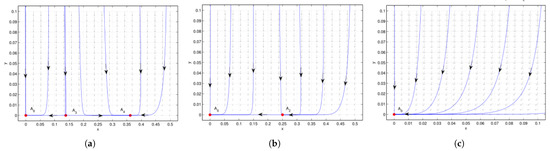
Figure 1.
Case 1 of (no positive equilibrium), is a stable node. (a) , is a saddle, and is a stable node. (b) , is an attracting saddle node, with the stable parabolic (hyperbolic) domain located in the right (left) half plane. (c) , there is no extra boundary equilibrium besides the stable point , which implies the co-extinction of interacting species. We see that the system undergoes saddle-node bifurcation at when .
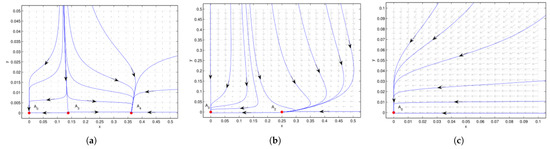
Figure 2.
Case 1 of (no positive equilibrium). is an attracting saddle node, with an attracting parabolic sector in the first quadrant. (a) , is a repelling saddle node with a hyperbolic sector in the first quadrant, and is an attracting saddle node, with its stable parabolic sector in the first quadrant. (b) , , is an attracting saddle node, with its stable parabolic (hyperbolic) sector located in the right (left) half plane. (c) , there is no extra boundary equilibrium besides the attracting saddle-node point , which implies the co-extinction of interacting species. We see that the system undergoes saddle-node bifurcation at when .
| Region | ||||
|---|---|---|---|---|
| (1) , (Figure 1a) | stable | - | saddle | stable |
| (2) , (Figure 1b) | stable | saddle node | - | - |
| (3) , (Figure 1c) | stable | - | - | - |
| (4) , (Figure 2a) | saddle node | - | saddle node | saddle node |
| (5) , (Figure 2b) | saddle node | saddle node | - | - |
| (6) , (Figure 2c) | saddle node | - | - | - |
Case 1 of .
We secondly consider the system (26) (a specific instance of system (5) where we have and , separately.
Example 2.
As shown in Figure 3 that trivial equilibrium of system (26) is a saddle, and boundary equilibrium is globally asymptotically stable, which implies the prey population collapse.
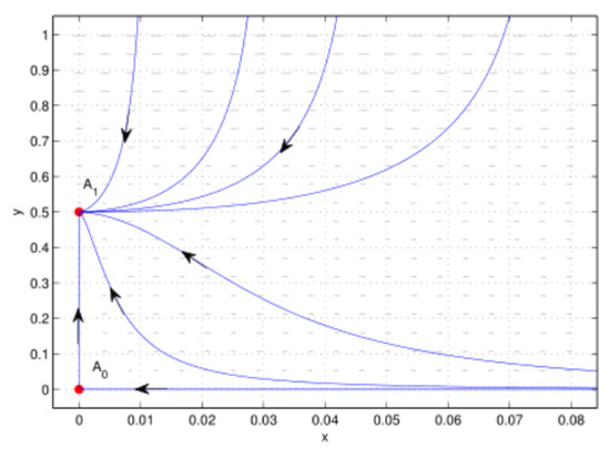
Figure 3.
Case 2 of , .
Thirdly, we consider the system (27) (a specific instance of system (5)) with , , separately. It is shown in Table 3 the dynamical behaviors of system (27) in regions (1)–(8).
Example 3.
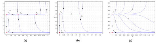
Figure 4.
Case 3 of , , is a saddle, is a stable node. (a) , is a saddle, while is a stable node. (b) , is an attracting saddle node, with stable parabolic (hyperbolic) domain located in the right (left) half plane. (c) , there is no interior equilibrium. We see that the system undergoes saddle-node bifurcation near .
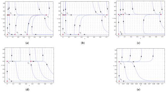
Figure 5.
Case 3 of , , is a saddle, is a stable node. (a) , is an unstable node, is a saddle. is a saddle, is a stable node. (b) , is a repelling saddle node, with a repelling parabolic (hyperbolic) sector located in the left (right) half plane. is a saddle, and is stable. (c) , is a saddle, and is stable. (d) , and is an attracting saddle node, with its stable parabolic (hyperbolic) domain located in the right (left) half plane. (e) , there is no interior equilibrium. We see that the system undergoes saddle-node bifurcation at when and when , respectively.
| Region | ||||||||
|---|---|---|---|---|---|---|---|---|
| (1) , (Figure 4a) | saddle | stable | - | - | - | stable | - | saddle |
| (2) , (Figure 4b) | saddle | stable | - | - | - | - | saddle node | - |
| (3) , (Figure 4c) | saddle | stable | - | - | - | - | - | - |
| (4) , (Figure 5a) | saddle | stable | - | unstable | saddle | stable | - | saddle |
| (5) , (Figure 5b) | saddle | stable | saddle node | - | - | stable | - | saddle |
| (6) , (Figure 5c) | saddle | stable | - | - | - | stable | - | saddle |
| (7) , (Figure 5d) | saddle | stable | - | - | - | - | saddle node | - |
| (8) , (Figure 5e) | saddle | stable | - | - | - | - | - | - |
Case 3 of , .
Fourthly, we consider the system (28) (a specific instance of system (5)) with , separately. It is shown in Table 4 the dynamical behaviors of system (28) in regions (1)–(4).
Example 4.
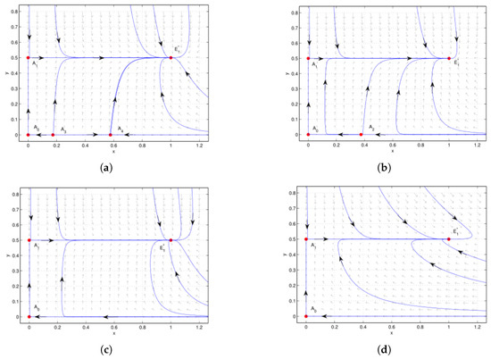
Figure 6.
Case 4 of , , is a saddle, is an attracting saddle node, with the hyperbolic sector located in the first quadrant (attracting parabolic sector in the left plane). (a) , , . is an unstable node, is a saddle. is globally asymptotically stable. (b) , , . is a repelling saddle node, with the repelling parabolic (hyperbolic) sector located in the left (right) half plane. is globally asymptotically stable. (c) , , . is globally asymptotically stable. (d) , , . is globally asymptotically stable. We see that the system undergoes saddle-node bifurcation near when .
| Region | ||||||||
|---|---|---|---|---|---|---|---|---|
| (1) , (Figure 6a) | saddle | saddle node | - | unstable | stable | stable | - | - |
| (2) , (Figure 6b) | saddle | saddle node | saddle node | - | - | stable | - | - |
| (3) , (Figure 6c) | saddle | saddle node | - | - | - | stable | - | - |
| (4) (Figure 6d) | saddle | saddle node | - | - | - | stable | - | - |
Case 4 of , .
Finally, we consider the system (29) (a specific instance of system (5)) with , , separately. It is shown in Table 5 the dynamical behaviors of system (29) in regions (1)–(4).
Example 5.
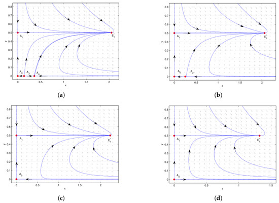
Figure 7.
Case 5 of , is a saddle, is a saddle: (a) , . is an unstable node, is a saddle. is globally asymptotically stable. (b) , . is a repelling saddle node, with repelling parabolic (hyperbolic) sector located in the left (right) half plane. is globally asymptotically stable. (c) , . is globally asymptotically stable. (d) , . is globally asymptotically stable. We see that the system undergoes saddle-node bifurcation at when .
5.2. Sensitivity Analysis of Parameter , and
Under suitable parameter conditions, we generate bifurcation diagrams in MATLAB R2012a by selecting either or the harvesting efforts , as bifurcation parameters to analyze how these parameters influence the existence and stability of equilibrium points in the system.
As illustrated in Figure 8a, for , the system exhibits two boundary equilibrium points: (unstable) and (stable). When , these two points merge into a single equilibrium , and for , no boundary equilibrium exists. This indicates that the system undergoes a saddle-node bifurcation at when .
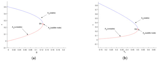
Similarly, Figure 8b shows that for , there are two boundary equilibria, (unstable) and (stable). At , they coalesce into , and for , no boundary equilibrium persists. Again, a saddle-node bifurcation occurs at when .
Figure 9a demonstrates that for , the system possesses two positive equilibrium points: (unstable) and (stable). At the critical value , these equilibria coalesce into a single point , and for , no positive equilibrium exists. This behavior clearly indicates a saddle-node bifurcation occurring at when .
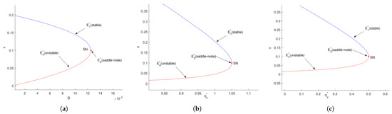
Figure 9.
(a) The bifurcation diagram of system (27) in the () plane, where we have , , , , separately. (b) The bifurcation diagram of system (27) in the () plane, where we have , , , , separately. (c) The bifurcation diagram of system (27) in the () plane, where we have , , , , separately. denotes a saddle-node bifurcation.
A similar bifurcation pattern is observed in Figure 9b. When , the system exhibits two boundary equilibrium points ( unstable and stable). These merge into at , and disappear completely for , confirming another saddle-node bifurcation at with .
The third case, shown in Figure 9c, reveals identical dynamical behavior with respect to . Two boundary equilibria ( and ) exist for , merge at , and vanish when , completing the trifecta of saddle-node bifurcations at under the condition .
6. Conclusions
The dynamical behavior of a commensalism model is quite complex after incorporating the Allee effect and non-selective harvest into the prey. System (5) exhibits variation in its boundary and interior equilibrium counts. As the parameters vary, the number of boundary and interior equilibrium solutions can transition from 0 to 1 to 2, leading to the occurrence of saddle-node bifurcations. Additionally, the prey population size at the interior equilibrium point of system (5) with globally asymptotic stability depends on the Allee parameter, and it satisfies the condition that , . By appropriately controlling the harvesting rate, the population density increases as the Allee effect intensifies. This phenomenon is quite rare and differs from most conclusions drawn from species groups influenced by the Allee phenomenon. When the prey harvesting constant is large enough, whereas predator harvesting remains regulated (), the prey species will ultimately approach population collapse. While the predator harvesting constant is large enough (), both species may ultimately approach population collapse. However, by controlling the harvesting parameter (, ), coexistence between the prey and predator can be achieved. Therefore, to ensure the sustainable survival of the populations, it is necessary to establish appropriate protected areas where species are free from harvesting, allowing both populations to sustainably develop under suitable conditions.
Remark
1. This study simplifies ecological complexity: (1) populations are assumed to be homogeneous, ignoring individual diversity (e.g., age and genetics) and spatial dynamics (e.g., migration and habitat fragmentation). Real-world spatial processes (resource distribution and dispersal) could alter stability or extinction risks but are not addressed. (2) Environmental randomness (e.g., climate fluctuations) and disturbances are excluded. Future work could integrate spatial models (reaction–diffusion frameworks) or stochastic elements to enhance realism. Despite these limitations, the results offer foundational insights into ecological mechanisms.
2. While this study provides theoretical insights into existence and stability of equilibria in a Lotka–Volterra commensalism system that incorporates the weak Allee effect in prey and symmetric non-selective harvesting, future work should extend these results to real-world applications. Potential directions include (1) the empirical testing of stability thresholds in controlled ecosystems (e.g., mesocosms or fisheries with symmetrical harvesting records), (2) comparative performance analysis against asymmetric harvesting policies using historical collapse events, and (3) the integration of machine learning techniques (e.g., deep neural networks) to optimize harvesting efforts under stochastic environments as demonstrated in epidemiological modeling [47]. Such applied studies would bridge the gap between our analytical criteria and sustainable resource management practices.
Author Contributions
Conceptualization, K.F. and F.C.; methodology, K.F. and Y.W.; software, K.F. and X.C.; validation, F.C. and X.C.; data curation, Y.W.; writing—original draft preparation, K.F.; writing—review and editing, K.F., F.C. and X.C.; supervision, F.C. and X.C.; funding acquisition, K.F. and F.C. All authors have read and agreed to the published version of the manuscript.
Funding
This work was financially supported through Science and Technology Program for Middle-aged and Young Scholars of Fujian Provincial Department of Education Fujian Province (No. JAT220511), Natural Science Foundation of Fujian Province (No. 2024J01273) and (No. 2023J01163), and Science and Education Innovation Group Cultivation Project of Fuzhou University Zhicheng College (No. ZCKC23005).
Data Availability Statement
All research outcomes and novel contributions have been comprehensively presented in this manuscript. Further details may be obtained by contacting the corresponding author.
Acknowledgments
We extend our sincere appreciation to the editorial team and peer anonymous referees for their constructive feedback that led to substantial improvements in this study.
Conflicts of Interest
The research team confirms there are no known conflicts of interest, including financial or personal factors, that could influence these findings.
References
- Ditta, A.; Naik, P.A.; Ahmed, R.; Huang, Z.X. Exploring periodic behavior and dynamical analysis in a harvested discrete-time commensalism system. Int. J. Dyn. Control. 2025, 13, 63. [Google Scholar] [CrossRef]
- Chen, F.D.; Chen, Y.M.; Li, Z.; Chen, L.J. Note on the persistence and stability property of a commensalism model with Michaelis-Menten harvesting and Holling type II commensalistic benefit. Appl. Math. Lett. 2022, 134, 108381. [Google Scholar] [CrossRef]
- Osuna, O.; Villavicencio-Pulido, G. A seasonal commensalism model with a weak Allee effect to describe climate-mediated shifts. Geiser. Sel. Mat. 2024, 11, 212–221. [Google Scholar] [CrossRef]
- Qu, M.Z. Dynamical analysis of a Beddington-DeAngelis commensalism system with two time delays. J. Appl. Math. Comput. 2023, 69, 4111–4134. [Google Scholar] [CrossRef]
- Cai, J.N.; Pinto, M.; Xia, Y.H. Stability and Bifurcation Analysis of a Commensal Model with Allee Effect and Herd Behavior. Open Math. 2022, 32, 1. [Google Scholar] [CrossRef]
- Patra, R.R.; Maitra, S. Dynamics of stability, bifurcation and control for a commensal symbiosis model. Int. J. Dyn. Control 2024, 12, 2369–2384. [Google Scholar] [CrossRef]
- Liu, X.W.; Yue, Q. Stability property of the boundary equilibria of a symbiotic model of commensalism and parasitism with harvesting in commensal populations. AIMS Math. 2022, 7, 18793–18808. [Google Scholar] [CrossRef]
- Xu, L.L.; Xue, Y.L.; Xie, X.D.; Lin, Q.F. Dynamic Behaviors of an Obligate Commensal Symbiosis Model with Crowley–Martin Functional Responses. Axioms 2022, 11, 298. [Google Scholar] [CrossRef]
- Xu, L.L.; Xue, Y.L.; Lin, Q.F.; Lei, C.Q. Positive periodic solution of a discrete Lotka-Volterra commensal symbiosis model with Michaelis–Menten type harvesting. WSEAS Trans. Math. 2022, 21, 515–523. [Google Scholar]
- Wei, Z.; Xia, Y.H.; Zhang, T.H. Stability and bifurcation analysis of a commensal model with additive Allee effect and nonlinear growth rate. Internat. J. Bifur. Chaos. 2021, 13, 2150204. [Google Scholar] [CrossRef]
- Xue, Y.L.; Xie, X.D.; Lin, Q.F.; Chen, F.D. Almost periodic solutions of a commensalism system with Michaelis-Menten type harvesting on time scales. Open Math. 2019, 17, 1503–1514. [Google Scholar] [CrossRef]
- Chen, B.G. The influence of commensalism on a Lotka-Volterra commensal symbiosis model with Michaelis-Menten type harvesting. Adv. Differ. Equ. 2019, 2019, 43. [Google Scholar] [CrossRef]
- Deng, H.; Huang, X. The influence of partial closure for the populations to a harvesting Lotka-Volterra commensalism model. Commun. Math. Biol. Neurosci. 2018, 2018, 10. [Google Scholar]
- Han, R.Y.; Chen, F.D. Global stability of a commensal symbiosis model with feedback controls. Commun. Math. Biol. Neurosci. 2015, 2015, 15. [Google Scholar]
- Gao, W.J.; Jia, X.; Shi, R.Q. Dynamics and optimal harvesting for fishery models with reserved areas. Symmetry 2024, 16, 800. [Google Scholar] [CrossRef]
- Moustafa, E.; Mahmoud, M. Dynamics of a Fractional-Order Eco-Epidemiological Model with Two Disease Strains in a Predator Population Incorporating Harvesting. Axioms 2025, 14, 53. [Google Scholar]
- He, M.X.; Li, Z. Bifurcation of a Leslie–Gower Predator–Prey Model with Nonlinear Harvesting and a Generalist Predator. Axioms 2024, 13, 704. [Google Scholar] [CrossRef]
- García, C.C. Bifurcations on a discontinuous Leslie-Grower model with harvesting and alternative food for predators and Holling II functional response. Commun. Nonlinear Sci. Numer. Simul. 2023, 116, 106800. [Google Scholar] [CrossRef]
- Kashyap, A.J.; Zhu, Q.X.; Sarmah, H.K.; Bhattacharjee, D. Dynamical study of a predator–prey system with Michaelis–Menten type predator-harvesting. Int. J. Biomath. 2023, 16, 2250135. [Google Scholar] [CrossRef]
- Wu, H.; Li, Z.; He, M.X. Bifurcation analysis of a Holling-Tanner model with generalist predator and constant-yield harvesting. Int. J. Bifurc. Chaos. 2024, 34, 2450076. [Google Scholar] [CrossRef]
- Xu, Y.C.; Yang, Y.; Meng, F.W.; Ruan, S.G. Degenerate codimension-2 cusp of limit cycles in a Holling-Tanner model with harvesting and anti-predator behavior. Nonlinear Anal. Real World Appl. 2024, 76, 103995. [Google Scholar] [CrossRef]
- Allee, W.C. Animal Aggregations: A Study in General Sociology; University of Chicago Press: Chicago, IL, USA, 1932. [Google Scholar]
- Kuussaari, M.; Saccheri, I.; Camara, M.; Hanski, I. Allee effect and population dynamics in the glanville fritillary butterfly. Oikos 1998, 82, 384–392. [Google Scholar] [CrossRef]
- Stephens, P.A.; Sutherl, W.J. Consequences of the Allee effect for behaviour, ecology and conservation. Trends Ecol. Evol. 1999, 14, 401–405. [Google Scholar] [CrossRef] [PubMed]
- Courchamp, F.; Grenfell, B.; Clutton-Brock, T. Population dynamics of obligate cooperators. Proc. R. Soc. Lond. B 1999, 266, 557–563. [Google Scholar] [CrossRef]
- Manoj, K.S.; Arushi, S.; Luis, M.S. Dynamical complexity of modified Leslie–Gower predator—Prey model incorporating double Allee effect and fear effect. Symmetry 2024, 16, 1552. [Google Scholar]
- Chen, F.D.; Li, Z.; Pan, Q.; Zhu, Q. Bifurcations in a Leslie–Gower predator—Prey model with strong Allee effects and constant prey refuges. Chaos Solitons Fract. 2025, 192, 115994. [Google Scholar] [CrossRef]
- Chen, S.M.; Chen, F.D.; Srivastava, V.; Parshad, R.D. Dynamical analysis of a Lotka-Volterra competition model with both Allee and fear effects. Int. J. Bifurc. Chaos. 2024, 17, 2350077. [Google Scholar] [CrossRef]
- Wang, F.; Yang, R. Dynamics of a delayed reaction–diffusion predator–prey model with nonlocal competition and double Allee effect in prey. IInt. J. Biomath. 2023, 1, 2350097. [Google Scholar] [CrossRef]
- González-Olivares, E.; Rojas-Palma, A. Influence of the strong Allee effect on prey and the competition among predators in Leslie-Gower type predation models. Int. J. Bifurcat. Chaos. 2020, 7, 302–313. [Google Scholar] [CrossRef]
- Cruz, R.L. Stability of a Leslie-Gower type predator-prey model with a strong Allee effect with delay. Sel. Mat. 2022, 9, 24–33. [Google Scholar] [CrossRef]
- Wang, F.; Yang, R.; Zhang, X. Turing patterns in a predator–prey model with double Allee effect. Math. Comput. Simul. 2024, 220, 170–191. [Google Scholar] [CrossRef]
- Luo, D.; Wang, Q. Global dynamics of a Holling-II amensalism system with nonlinear growth rate and Allee effect on the first species. Int. J. Bifurc. Chaos 2021, 31, 2150050. [Google Scholar] [CrossRef]
- Guan, X.Y.; Liu, Y.; Xie, X.D. Stability analysis of a Lotka-Volterra type predator-prey system with Allee effect on the predator species. Commun. Math. Biol. Neurosci. 2018, 2018, 9. [Google Scholar]
- Zhu, Q.; Chen, F.D. Impact of fear on searching efficiency of first species: A two species Lotka-Volterra competition model with weak Allee effect. Qual. Theory Dyn. Syst. 2024, 23, 143. [Google Scholar] [CrossRef]
- Fang, K.; Zhu, Z.L.; Chen, F.D.; Li, Z. Qualitative and Bifurcation Analysis in a Leslie-Gower Model with Allee Effect. Qual. Theory Dyn. Syst. 2022, 21, 86. [Google Scholar] [CrossRef]
- Fang, K.; Chen, J.B.; Zhu, Z.L. Qualitative and Bifurcation Analysis of a Single Species Logistic Model with Allee Effect and Feedback Control. IAENG Int. J. Appl. Math. 2022, 52, 220201. [Google Scholar]
- Liu, Y.Y.; Wei, J.J. Spatiotemporal dynamics of a modified Leslie-Gower model with weak Allee effect. Int. J. Bifurcat. Chaos. 2020, 30, 2050169. [Google Scholar] [CrossRef]
- Liu, H.Y.; Yu, H.G.; Dai, C.J.; Ma, Z.L.; Wang, Q.; Zhao, M. Dynamical analysis of an aquatic amensalism model with non-selective harvesting and Allee effect. Min. Math. Biosci. Eng. 2021, 18, 8857–8882. [Google Scholar] [CrossRef]
- Wei, Z.; Xia, Y.H.; Zhang, T.H. Stability and bifurcation analysis of an Amensalism model with weak Allee effect. Qual. Theor. Dyn. Syst. 2020, 23, 1–19. [Google Scholar] [CrossRef]
- Lin, Q.F. Stability analysis of a single species logistic model with Allee effect and feedback control. Adv. Differ. Equ. 2018, 2018, 190. [Google Scholar] [CrossRef]
- Mustafa, N.; Rahman, J.U.; Ishtiaq, U.; Popa, I.L. Artificial Neural Network-Based Approach for Dynamic Analysis and Modeling of Marburg Virus Epidemics for Health Care. Symmetry 2025, 17, 578. [Google Scholar] [CrossRef]
- Chen, F.D. On a nonlinear non-autonomous predator-prey model with diffusion and distributed delay. Commun. Math. Biol. Neurosci. 2005, 180, 33–49. [Google Scholar]
- Zhang, Z.F.; Ding, T.R.; Huang, W.Z.; Dong, Z.X. Qualitative Theory of Differential Equation; Translation of Mathematical Monographs; American Mathematical Society: Providence, RI, USA, 1992. [Google Scholar]
- Chen, L.S. Mathematical Models and Methods in Ecology; Scienec Press: Beijing, China, 1988. [Google Scholar]
- Perko, L. Differential Equations and Dynamical Systems; Springer: New York, NY, USA, 2013. [Google Scholar]
- Mustafa, N.; Rahman, J.U.; Omame, A. Modelling of Marburg virus transmission dynamics: A deep learning-driven approah with the efect of quarantine and health awareness interventions. Model. Earth Syst. Environ. 2024, 10, 7337–7357. [Google Scholar] [CrossRef]
Disclaimer/Publisher’s Note: The statements, opinions and data contained in all publications are solely those of the individual author(s) and contributor(s) and not of MDPI and/or the editor(s). MDPI and/or the editor(s) disclaim responsibility for any injury to people or property resulting from any ideas, methods, instructions or products referred to in the content. |
© 2025 by the authors. Licensee MDPI, Basel, Switzerland. This article is an open access article distributed under the terms and conditions of the Creative Commons Attribution (CC BY) license (https://creativecommons.org/licenses/by/4.0/).