Deep Learning-Based Optimal Condition Monitoring System for Plant Growth in an Indoor Smart Hydroponic Greenhouse

Abstract

This study introduces a deep learning (DL)-based optimal condition monitoring and control system tailored to indoor smart greenhouses, with a novel focus on maintaining symmetry—defined as a dynamic equilibrium among temperature, humidity, and CO₂ levels—critical in plant growth. A hydroponic greenhouse prototype was developed to capture real-time climate data at high temporal resolution. A custom 1D convolutional neural network (1D-CNN) optimized via a genetic algorithm (GA) was employed to predict environmental fluctuations, achieving R² scores up to 0.99 and a standard error of prediction (SEP) as low as 0.35%. The system then actuated climate control mechanisms to restore and maintain symmetry. Experimental validation revealed that plants grown under the symmetry-aware control system exhibited significantly improved growth metrics. The results underscore the potential of integrating symmetry-aware DL strategies into precision agriculture in achieving sustainable and resilient plant production systems.

1. Introduction

The growing global demand for food and the pressures of climate variability necessitate sustainable agricultural innovation. Indoor smart greenhouses offer a viable solution by enabling precise control over environmental conditions. Recent advances in artificial intelligence (AI), particularly deep learning (DL), have opened up new pathways for optimizing these controlled environments. One underexplored but critical aspect in this optimization is the inherent symmetry and balance among environmental parameters such as temperature, humidity, and carbon dioxide (CO₂) concentration. Deviations or asymmetries in these factors can lead to significant discrepancies in plant health, yield, and disease resistance. By treating these parameters not as independent variables but as components of a balanced system, we can utilize DL not only for prediction but also for restoring and maintaining environmental symmetry, thereby fostering optimal growth conditions.

In recent years, artificial intelligence (AI)—especially deep learning (DL)—has been increasingly applied to agricultural monitoring and control tasks due to its capacity to learn complex patterns from high-dimensional data. Numerous studies have applied DL to problems such as crop yield prediction, plant disease classification, and soil health monitoring [1,2,3,4,5,6]. However, most of these applications focus on field crops or isolated tasks, and only a limited number have been adapted to the controlled environments of greenhouses. Even among greenhouse-focused works, the emphasis is often placed solely on the time-series forecasting of individual parameters without incorporating these predictions into a closed-loop control system. A few studies have explored greenhouse environmental prediction using DL models. For instance, Jung et al. [7] evaluated time-series DL architectures like LSTM and GRU for temperature and humidity prediction in outdoor greenhouses. Similarly, van Mourik et al. [8] proposed model-based filtering for climate control using physics-informed models. While promising, these approaches were not designed for real-time control or for systems with multivariate coordination. Weldeslasie et al. [9] developed an automated climate monitoring system for flower greenhouses in Ethiopia, reporting strong performance using Advantech PC-card hardware, but again focused on monitoring rather than active control. Gong et al. [10] introduced a hybrid RNN–TCN model for crop yield prediction under greenhouse conditions, further emphasizing the importance of temporal features. Other works, such as [11], have demonstrated the value of integrating wireless sensor networks (WSNs) to automate monitoring, though most stopped short of integrating DL-based control frameworks. However, most control strategies still rely on static thresholds or rule-based automation, which lack adaptability [12,13,14].

In recent years, several advanced deep learning frameworks have emerged for optimizing greenhouse environments under climate variability. For example, a Transformer-based model, Trans-Farmer, has been proposed to learn complex hidden relationships among environmental and control variables, enabling the direct prediction of actuator settings in greenhouses with limited computational resources [15]. Similarly, the AI-GECS system, developed in Taiwan, integrates real-time meteorological data into gridded weather forecasts and employs a hybrid CLSTM–CNN–BP architecture to control greenhouse cooling operations based on predicted crop stress [16]. Another recent advancement, the Power-LSTM (PLSTM) model, has demonstrated exceptional performance in predicting greenhouse temperatures, achieving R² values up to 0.9999, outperforming standard DL models such as GRU and LSTM-RNN in a Spanish case study [17]. These studies collectively underline the rapid advancement of DL-driven greenhouse control systems and provide a foundation for exploring lightweight and symmetry-aware control frameworks such as the one proposed in this study. Our previous work [18] contributed to this domain by comparing deep neural networks (DNNs), long short-term memory (LSTM), and 1D convolutional neural networks (1D-CNNs) for the short-term prediction of temperature, humidity, and CO₂ concentration in hydroponic environments. The study highlighted the importance of time-step selection and revealed that DL models—particularly LSTM—can effectively capture short-term temporal dependencies. However, the study did not incorporate real-time control or address the underlying structural interdependence among environmental variables. One of the key conceptual innovations in this research is the notion of environmental symmetry—the idea that plant growth is optimized not just by maintaining target values for each variable but by preserving a balanced state across all relevant environmental parameters. We define symmetry as the dynamic equilibrium among temperature, humidity, and CO₂ within specified threshold bands centered on optimal setpoints. A loss of symmetry—referred to as environmental asymmetry—can degrade plant health, even if individual values remain within acceptable ranges. This concept is largely absent from prior works, which often treat control variables independently and ignore their co-regulation.

To address these gaps, we propose a novel deep learning-based environmental monitoring and control system for indoor hydroponic smart greenhouses that introduces three main innovations:

• Symmetry-aware environmental control: We formulate plant growth optimization as a problem of maintaining environmental symmetry, rather than independent parameter regulation.
• Genetic Algorithm (GA)-optimized 1D-CNN architecture: We employ a lightweight, high-accuracy model that uses an evolutionary search to automatically tune hyperparameters for improved performance and training efficiency.
• Real-time autonomous control framework: The system is implemented on a Jetson Nano platform and directly actuates fans, CO₂ injectors, and dehumidifiers to dynamically restore symmetry when deviations are predicted.

This paper is organized as follows: Section 2 details the architecture of the proposed DL model and the real-time control system. Section 3 presents the experimental setup and environmental data acquisition in the hydroponic greenhouse. Section 4 discusses the performance comparison of DL models and the effectiveness of symmetry-aware control. Section 5 concludes the study with insights into practical applications and future work directions.

2. Methodology

2.1. A Novel DL Model for Environmental Predictions

Deep Convolutional Neural Network (CNN) architectures are instrumental in acquiring hierarchical features, crucial in achieving enhanced prediction accuracy. However, the increasing complexity of such architectures poses challenges in attaining optimal training due to issues associated with gradient information flow during back-propagation. To address this challenge, this study introduces the 1D-CNN block based on direct connections for forecasting climate parameters within an indoor smart greenhouse setting. The direct connection method with two convolutional layers is displayed in Figure 1. This block serves the dual purpose of improving gradient information flow, diminishing the count of trainable parameters, and reducing the optimization time of the network architecture [19].

The foundational element of the overall novel DL model architecture is the 1D-CNN block, designed to optimize the flow of gradient information by strengthening connections between different convolution layers while simultaneously reducing the number of trainable parameters. Within this block, a 1-dimensional convolution layer is employed to extract localized features from the input data, facilitating the extraction of high-level features from the input row vector. Kernels, acting as filters, serve as the parameters of the convolutional layer, convolving the input row vector with each filter during the feed-forward operation. The resulting convolutional layers generate feature maps that maintain spatial information while diminishing the temporal dimension of the signal.

The convolutional layer can be mathematically expressed as follows:

$$X_v^l=F\left({\sum }_{u\in M_v}{X}_u^{l-1}{K}_v^l+B_v^l\right),$$

(1)

where $X$ denotes the input vector, $X_v^l$ represents the updated feature maps produced by the convolution layer, $l$ stands for $l\mathrm{th}$ layer of the network, $X_u^{l-1}$ represents $u\mathrm{th}$ feature maps produced by the $(l-1)\mathrm{th}$ layer, $K_v^l$ represents a convolutional filter, and $B_v^l$ denotes the bias in the convolution operation.

A batch normalization (BN) layer is methodically integrated, where the normalization process involves subtracting the mean and dividing by the standard deviation, subsequently adjusting the result through learnable parameters by scaling and shifting. Throughout training, BN maintains running averages of the mean and standard deviation for utilization during inference. The inclusion of the BN layer within the 1D-CNN block significantly contributes to the stability, speed, and efficacy of training deep neural networks. Notably, it addresses challenges such as internal covariate shift, expedites convergence, diminishes reliance on initialization, and alleviates issues associated with vanishing/exploding gradients. Subsequently to the BN layer, the output traverses an activation layer, and the resulting output is concatenated with the initial input data. This composite data undergoes an iterative process through the convolutional (Conv), BN, and activation layers. The output of this sequence is concatenated with both the initial input data and the preceding concatenated data. Following this stage, a dimension reduction module is applied, encompassing four layers: a convolutional layer with a 1 × 1 filter size for a depth-wise reduction in input data, as shown in Figure 2, batch normalization, an activation layer, and a pooling layer for a width-wise reduction in data.

Max pooling, a widely employed pooling operation in 1D-CNNs, is utilized, wherein the maximum value within a pooling window is selected as the representative value. This strategy aids in preventing overfitting within the network. The mathematical expression for the pooling operation is articulated as follows:

$$a_{v-s}^l=f\left(W_v^{l}down\left(M_v^{l-1}\right)+B_v^l\right),$$

(2)

where $W_v^l$ represents the weight vector, $down\left(·\right)$ denotes the pooling operation, and $M_v$ presents the feature maps produced by pooling operations.

Subsequently to the application of the 1D-CNN blocks, as shown in Figure 3a, the resultant feature maps undergo flattening, wherein they are transformed into a one-dimensional vector. This operation effectively condenses the spatial dimensions into a singular dimension, facilitating the data’s readiness for engagement with the fully connected layers within the adaptive DL model architecture. The fully connected layers are characterized by densely connected neurons that discern intricate relationships among the extracted features. The potential introduction of additional dimensionality changes is contingent upon the specific architectural design and the quantity of neurons in each layer. Following this transformation, the output layer, comprising three neurons, receives a one-dimensional vector emanating from the fully connected layer. This vector is instrumental in formulating the ultimate prediction for the climate parameters within the indoor smart greenhouse, as visually represented in Figure 3b. In our 1D-CNN block, we used a kernel size of 3, stride of 1, and ‘same’ padding to preserve the input dimension across layers. These settings were chosen to ensure efficient feature extraction while maintaining temporal resolution, which is important for the accurate time-series forecasting of environmental parameters.

2.2. Hyperparameter Optimization of the Proposed DL Model

The genetic algorithm (GA) is frequently employed to address optimization challenges, particularly in scenarios characterized by numerous local optima or a substantial number of factors. Within the framework of GAs, the parameters subject to optimization are designated as chromosomes. The GA initializes the process by generating random chromosomes until the desired set is achieved, encompassing four primary operations. Initially, the fitness value of each chromosome is computed. Subsequently, the selection operator identifies robust chromosomes based on their fitness. Thirdly, the crossover operator partitions existing chromosomes, generating novel configurations. Lastly, these chromosomes undergo random mutation to introduce further diversity. The fitness of the newly formed chromosomes is subsequently evaluated in the ensuing cycle, and this iterative process continues until the desired outcomes are achieved. However, within the domain of deep learning, training a GA model poses computational challenges as the fitness of chromosomes is evaluated after each iteration. Therefore, achieving optimal chromosomes in fewer iterations becomes imperative. This is accomplished through the enhancement and optimization of GAs. Although the concept of modifying GAs is not novel, several scholars have proposed refinements tailored to specific tasks and applications. In this study, our focus lies in optimizing common GA operators to better align with our framework.

Salient advancements encompass:

• The recognition that not every mutated chromosome surpasses its unmutated counterparts, as dictated by the selection operator. Consequently, preference is given to the most optimal chromosomes from both recent and previous generations.
• The implementation of adaptive crossover probability in the crossover operator, departing from a fixed value.
• The mitigation of the risk of losing advantageous genes due to mutation operators.

The adaptive deep neural network based on the 1D-CNN block and its hyperparameters are optimized simultaneously using GA. The hyperparameters of the neural network and their ranges and optimal results are listed in

Table 1. The best hyperparameters obtained by GA.

No.	Hyperparameters	Ranges	Optimal Results
1	Number of blocks	[1, 7]	2
2	Number of filters	[8, 256]	32
3	Filter size	[3, 7]	3
4	Number of neurons	[10, 200]	35
5	Learning rate	[0.00001, 0.01]	0.00092
6	Activation functions	[relu, tanh, sigmoid, LeakyReLU, selu, elu]	relu
7	Optimizers	[SGD, Adam, RMSprop, Adadelta, Adagard, Adamax, Nadam]	Adam
8	Number of filters for dimension reduction module 1	[8, 256]	16
9	Number of filters for dimension reduction module 2	[8, 256]	8
10	Batch size	[4, 256]	64
11	Number of epochs	[20, 200]	42

. The objective function of GA is the loss function, which is expressed in Equation (3). The root mean square error (RMSE) function is used as a loss function for the proposed adaptive DL model.

$$RMSE=\sqrt{{\displaystyle \frac{\sum _{i=1}^N{(x_i-y_i)}^2}{N}}},$$

(3)

where $x_i$ is the predicted value, $y_i$ is the true value, and $N$ is the number of samples.

As mentioned earlier, the primary objective of this study was to design an adaptive 1D-CNN block-based DL architecture for climate parameters (temperature, humidity, and CO₂) prediction, determining the optimal number of CNN layers and other hyperparameters. The GA utilized in this context incorporates specific parameters: the maximum number of generations is set to 20, and the probabilities of crossover and mutation are 0.4 and 0.2, respectively.

2.3. Environmental Monitoring System

This section provides an exhaustive analysis of the AI-based autonomous system implementation, crafted by integrating Jetson Nano. At the core of this system is a Jetson Nano controller-based hardware arrangement strategically deployed within the hydroponics greenhouse field. This hardware setup diligently gathers plant-related data, leveraging an array of sensors. Subsequently, all the data garnered from these sensors is seamlessly transmitted for storage and analysis. An essential component of this architecture is the integration of an artificial intelligence system. This AI system is fortified with the proposed DL model. Its continuous vigilance entails monitoring sensor data and evaluating the health status of plants.

A Jetson Nano implements the planned AI-based autonomous system, various actuators, and an environmental sensor. The system regulates variables, such as temperature, humidity, and CO₂ levels. In the memory of the Jetson Nano, sensor readings are also updated continuously. The SCD40 sensor is used to gauge atmospheric variables, such as CO₂ levels, humidity, and temperature. The proposed DL model successfully predicts temperature, humidity, and CO₂ in this scenario after predetermined time intervals. The predicted variables can be used in a control strategy to change and regulate various environmental parameters dynamically inside the smart greenhouse, as shown in Figure 4. For example, the control system can activate or deactivate cooling equipment (fans) based on the predicted temperature to maintain the ideal temperature range for crop growth after comparison with thresholds, because maintaining an optimal temperature range allows for the efficient functioning of photosynthesis. Most plants have specific temperature preferences for optimal growth, and controlling the temperature helps ensure that these conditions are met. Proper humidity levels prevent excessive transpiration, reducing water stress on plants. This helps maintain optimal turgor pressure in plant cells, promoting growth and ultimately leading to higher crop yields. Therefore, the dehumidifier installed inside of the smart greenhouse is activated or deactivated by the control system to maintain the ideal humidity range for crop growth after comparison with thresholds. Increasing CO₂ levels in the smart greenhouse enhances the rate of photosynthesis, leading to improved nutrient uptake by plants. This can result in better growth, development, and overall plant health. Therefore, the CO₂ generator installed inside the smart greenhouse is activated or deactivated by the control system to maintain the ideal CO₂ concentration level range for crop growth after comparison with thresholds.

An automated and optimal environment for crop production is developed by incorporating the expected factors into a control strategy. This immediately affects crop growth because a favorable climate is essential in increasing yields, lowering the risk of illness, and improving crop quality. Photosynthesis, transpiration, and nutrient uptake are just a few of the physiological processes in plants that can be impacted by the precise management of temperature, humidity, and CO₂ levels. Strong plant development, improved resource efficiency, and increased crop output can be achieved by keeping these factors within the ideal range.

3. Experimental Setup

3.1. Prototype of Smart Hydroponic Greenhouse

In pursuit of advancing sustainable and technologically driven agriculture, the following experimental setup has been meticulously designed to create a state-of-the-art smart hydroponic smart greenhouse prototype. The innovative integration of various sensors, control systems, and monitoring tools serves as a testament to the potential of modern technology in enhancing smart greenhouse agriculture. The experiment is conducted in the indoor hydroponic smart greenhouse shown in Figure 5 with a 50 × 50 × 60 cm experimental space. A completely automated indoor hydroponic smart greenhouse design includes several steps, including detecting plants and insects, forecasting the environment, AI-based decision-making, and automation. The experimental setup is housed within a specially designed hydroponic smart greenhouse, a controlled environment that enables precise cultivation practices. This smart greenhouse provides a controlled ecosystem for plant growth and experimentation.

Our proposed AI-based controlling system focuses on maintaining an optimal environment in the smart greenhouse for healthy crop production. Therefore, the sensor measures temperature, humidity, and CO₂ levels, and the proposed DL model forecasts these values after certain time intervals. Based on these predictions, the controlling system compares thresholds of temperature, humidity, and CO₂ levels and takes action to activate or deactivate fans, dehumidifiers, and CO₂ generators. The thresholds are selected and set up for plant types inside the smart greenhouse.

3.2. Environmental Parameter Dataset of Smart Greenhouse

The temperature, humidity, and CO₂ levels were measured every minute in an indoor hydroponic smart greenhouse for one week (16 March–23 March 2023), which served as the data collection period. A sensor (Model: SCD40) was positioned inside the smart greenhouse and connected to a data collecting system is used to gather the dataset. The sensor specification is listed in

Table 2. Technical specification of the sensor.

Name	Specification
Built-in chip	Sensirion SCD40
Measurement	Temperature, humidity, and CO2
Temperature measuring range	−10 °C to 60 °C
Measurement accuracy	±0.8 °C
Humidity measuring range	0% to 95% RH
Measurement accuracy	±6% RH
CO2 measurement range	400 ppm to 2000 ppm
Measurement accuracy	±50 ppm + 5%
Dimensions	24 × 24 × 16 mm
Module weight	7.54 g

. Four distinct time intervals, i.e., 1, 5, 10, and 15 min, were used to partition the dataset for comparison study to find the best time interval for the smart greenhouse. The dataset underwent preprocessing to eliminate any outliers and missing values. In preprocessing, the dataset was also normalized to make the range between 0 and 1. A data preprocessing method called normalization was used to convert the values of features in a dataset to a standard scale. This was performed to make data modeling and analysis easier, as well as to lessen the effect of size differences on the precision of machine learning models. A scaling technique called normalization shifts and rescales values so that they fall between the ranges of 0 and 1. It is also called Min-Max scaling. The normalizing formula is expressed in Equation (4):

$$X^{\prime }={\displaystyle \frac{X-X_{min}}{X_{max}-X_{min}}},$$

(4)

where $X_{max}$ and $X_{min}$ denote the maximum and minimum values of feature, respectively. The numerator will be zero when the value of $X$ is the lowest number in the column; hence, $X^{\prime }$ will be 0. The numerator is equal to the denominator, but, when the value of $X$ is the highest value in the column, as a result, the value of $X^{\prime }$ is 1. The value of $X^{\prime }$ is between 0 and 1 if the value of $X$ is between the lowest and maximum value.

Following this, the datasets are split into training and testing datasets, with training datasets using 80% of the data and testing datasets using 20% of the data. Detailed information about datasets is given in

Table 3. Partition of all datasets.

Time Interval (Minutes)	Total Number of Data Samples	Training Samples	Testing Samples
1	11,683	9346	2337
5	2336	1869	467
10	1167	934	233
15	778	623	155

. The pertinent features for the deep learning models are extracted by conducting feature engineering on the dataset. The retrieved features included lagged temperature, humidity, and CO₂ levels. The deep learning models including DNN, LSTM, 1D-CNN, and the proposed adaptive DL models receive these features as an input.

4. Results and Discussion

4.1. Performance Metrics

DL models can predict environmental parameters, such as temperature, humidity, and CO₂ concentration. In order to evaluate the performance of DL models, two very common performance metrics have been used. The first one is the coefficient of determination (R²), which assesses the correlation between the expected and observed data. The second one is the percent standard error of prediction (% SEP). These measures aid in evaluating the model’s ability to account for variations between anticipated and observed values [20]. These computations’ formulas are provided in Equations (5) and (6),

$$R^2=1-{\displaystyle \frac{SSE}{SSTO}}=1-{\displaystyle \frac{\sum _{i=1}^N{\left(x_i-y_i\right)}^2}{\sum _{i=1}^N{\left(x_i-{\bar{x}}_i\right)}^2}},$$

(5)

$$SEP\left(\%\right)={\displaystyle \frac{100}{{\bar{x}}_i}}\sqrt{{\displaystyle \frac{\sum _{i=1}^N{\left(x_i-y_i\right)}^2}{N}}},$$

(6)

where $N$ is the total quantity of sets of data used in estimation; $x_i$ is the real temperature (measured output); $y_i$ is the forecast temperature (estimated output); $x{̄}_i$ is the mean value of the recorded outputs of the forecasting set; and SSTO assesses the variability of the mean observed values. An R² value near one and a (%) SEP value around zero are the ideal values for a perfect match between predicted and observed data.

4.2. Performance of DL Models

The results of the DNN model’s accuracy evaluation are shown in

Table 4. Comparison of the DNN model performance at different time intervals.

	DNN-1			DNN-5
	Temperature	Humidity	CO2	Temperature	Humidity	CO2
R2	0.98	0.96	0.81	0.99	0.95	0.97
SEP (%)	0.6	3.04	3.45	0.4	3.65	1.08
	DNN-10			DNN-15
	Temperature	Humidity	CO2	Temperature	Humidity	CO2
R2	0.95	0.94	0.81	0.98	0.93	0.91
SEP (%)	0.88	3.8	2.99	0.56	4.22	2.15

. Among all the parameters, the temperature displayed the best level of accuracy. DNN-1’s forecast of the temperature after one minute had an SEP of 0.6% and an R² of 0.98. With SEPs of 3.04% and 3.45% and R² values of 0.96 and 0.81, the predictions for humidity and CO₂ were significantly less accurate. When the time period was five minutes, DNN achieved its highest performance, with R² values of 0.99, 0.95, and 0.97, and SEPs of 0.4, 3.65, and 1.08 for temperature, humidity, and CO₂ levels, respectively. Additionally, the DNN-15 predictions outperformed the other models with SEPs of 0.56% for temperature, 4.22% for humidity, and 2.15% for CO₂.

The results of the LSTM and 1D-CNN models are presented in

Table 5. Comparison of the LSTM model performance at different time intervals.

	LSTM-1			LSTM-5
	Temperature	Humidity	CO2	Temperature	Humidity	CO2
R2	0.99	0.96	0.96	0.99	0.94	0.93
SEP (%)	0.4	3.09	1.35	0.46	3.54	1.77
	LSTM-10			LSTM-15
	Temperature	Humidity	CO2	Temperature	Humidity	CO2
R2	0.95	0.94	0.89	0.96	0.93	0.81
SEP (%)	0.94	3.85	2.38	0.84	4.18	3.17

and

Table 6. Comparison of the 1D-CNN model performance at different time intervals.

	1D-CNN-1			1D-CNN-5
	Temperature	Humidity	CO2	Temperature	Humidity	CO2
R2	0.96	0.96	0.97	0.95	0.93	0.92
SEP (%)	0.79	3.46	1.1	0.69	4.2	1.84
	1D-CNN-10			1D-CNN-15
	Temperature	Humidity	CO2	Temperature	Humidity	CO2
R2	0.97	0.95	0.74	0.88	0.94	0.74
SEP (%)	0.56	3.48	3.02	1.45	4.21	3.95

, respectively. The 1D-CNN model performed worse than LSTMs and DNN overall, but it performed marginally better than these two models at predicting CO₂ when the time interval was one minute. As an illustration, the temperature, humidity, and CO₂ were correctly predicted by 1D-CNN-1, with R² values of 0.96, 0.96, and 0.97, respectively. On the other hand, when the prediction time increased beyond five minutes, the accuracy of the 1D-CNN model dropped, and the prediction of temperature and CO₂ at the 15 min mark produced the worst results. The LSTM model, on the other hand, outperformed all other models in terms of predicted accuracy. The SEP and R² values for the temperature prediction made by the LSTM-5 were 0.46% and 0.99, respectively.

Table 7. Comparison of the proposed model performance at different time intervals.

	Proposed Model-1			Proposed Model-5
	Temperature	Humidity	CO2	Temperature	Humidity	CO2
R2	0.99	0.971	0.972	0.99	0.966	0.98
SEP (%)	0.35	2.87	0.89	0.35	3.28	0.92
	Proposed model-10			Proposed model-15
	Temperature	Humidity	CO2	Temperature	Humidity	CO2
R2	0.975	0.958	0.91	0.99	0.947	0.938
SEP (%)	0.43	3.44	1.33	0.47	3.76	1.77

presents the performance metrics of the proposed novel deep neural network model for temperature, humidity, and CO₂ prediction in a smart greenhouse environment for all time intervals. The proposed model consistently exhibits high R² values, ranging from 0.975 to 0.99, indicating a strong correlation between the predicted and actual temperature values. SEP percentages, ranging from 0.35% to 0.47%, indicate the precision of the proposed model in predicting temperature levels within the smart greenhouse. Similar trends are observed for humidity predictions across the proposed model. High R² values (>0.94) and SEP percentages emphasize the models’ accuracy in predicting humidity levels. The proposed model demonstrates robust performance in predicting CO₂ levels, with R² values exceeding 0.91. SEP percentages further affirm the accuracy of CO₂ predictions.

As the complexity of the proposed model increases from model-1 to model-15, there is a consistent enhancement in predictive performance, as evident from the improvement in R² values and SEP percentages. The proposed model showcases a high degree of accuracy in predicting temperature, humidity, and CO₂ levels within the smart greenhouse environment. The systematic increase in performance metrics with the complexity of the model indicates the effectiveness of the proposed approach. These findings lay a strong foundation for the reliable integration of AI-driven predictions into autonomous smart greenhouse control systems, contributing to the optimization of crop production conditions.

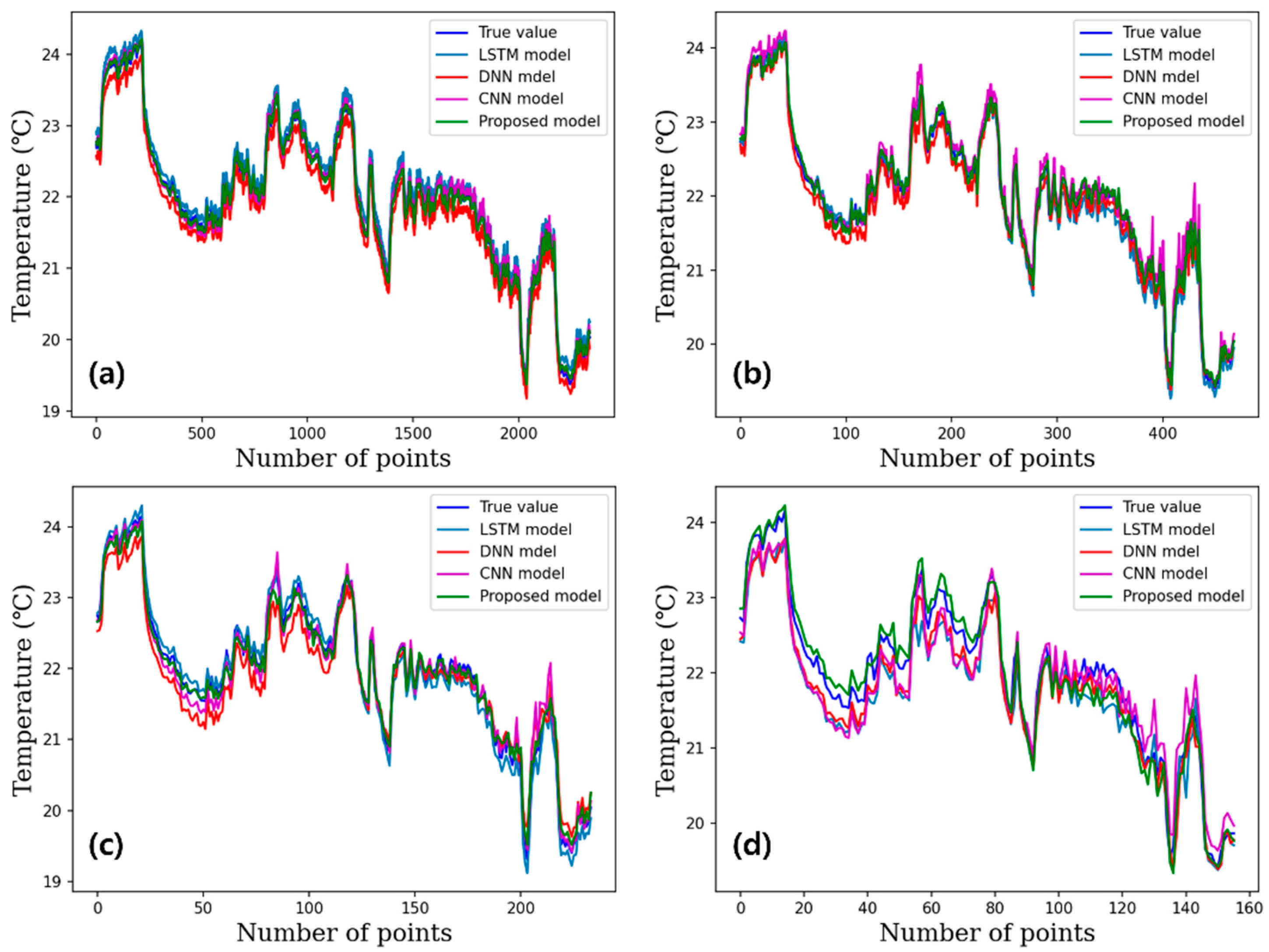
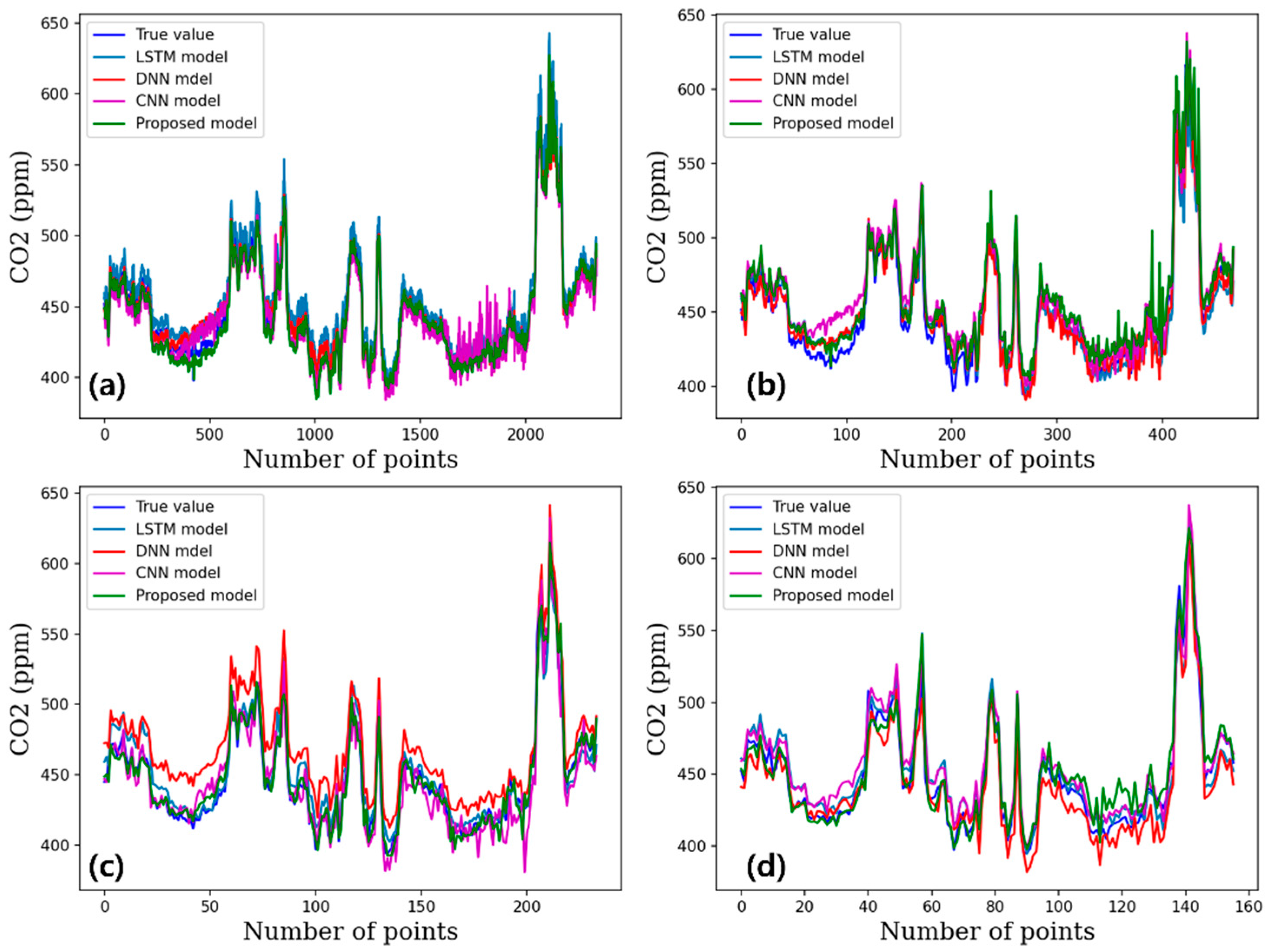
The effectiveness of the DNN, 1D-CNN, LSTM and the proposed novel DL model for forecasting temperature, humidity, and CO₂ levels over a range of time steps is shown in Figure 6, Figure 7 and Figure 8. All models are fairly accurate in predicting the temperature under all different climatic conditions, while predicting CO₂ level is challenging for all DL models. The graphs display each model’s prediction accuracy for temperature, humidity, and CO₂.

This study demonstrates how data-based modeling tools may be used to predict environmental changes in smart greenhouses. The performance of the proposed novel DL model is superior to that of the traditional neural network-based models. Therefore, it is advantageous to apply a more dynamic modeling technique that takes into account prior experiences in order to predict ongoing and recurring changes in the unique smart greenhouse environment. Similar conclusions have been reported by earlier research [21,22].

These results underline how crucial it is to pick the right time series deep learning model for predicting the environment in indoor hydroponic smart greenhouses. For precise time-interval predictions, the proposed novel DL model is the best option, whereas the DNN, 1D-CNN, and LSTM models have relatively poor accuracy. This study emphasizes the relevance of expanding the training dataset in order to enhance model performance. The use of numerous deep learning models, various time frames, and a variety of performance indicators for evaluation are some of this study’s strong points. For researchers and professionals in hydroponics and agriculture interested in utilizing deep learning models to anticipate the environment, the study also offers useful insights. However, there are certain restrictions on this study, as well. A hydroponic smart greenhouse’s long-term environment may not be accurately represented by the dataset utilized in the study, which is first limited to one week. Second, the study only considers three deep learning models; other models might be more effective in predicting the climate. Finally, the study ignored outside variables that might have an impact on the smart greenhouse climate, like weather and plant growth.

This study evaluates the effectiveness of various time series deep learning models to analyze climate predictions in indoor hydroponic smart greenhouses. The study sheds light on the models’ advantages and disadvantages and emphasizes the significance of choosing the right models for precise prediction. In order to enhance the effectiveness of the models, further studies should take external influences into account and employ larger datasets.

4.3. Experimental Confirmation

The utilization of the proposed DL-based control system in the smart greenhouse presents a stark contrast to traditional approaches lacking such sophisticated technology. The impact is evident across multiple facets of smart greenhouse management, fundamentally altering the dynamics of climate regulation, resource utilization, crop productivity, operational efficiency, and environmental sustainability. In the realm of climate regulation, the DL-based system takes the lead by dynamically optimizing environmental parameters such as temperature, humidity, and CO₂ levels based on real-time predictions. This control mechanism establishes and maintains an ideal climate for plant growth. In stark contrast, conventional smart greenhouse environments, often reliant on manual adjustments or basic automation, witness fluctuations that can deviate from the optimal range, potentially impacting plant health and growth. Resource utilization undergoes a transformative shift with the introduction of the DL-based control system. This system excels at precision in delivering water, nutrients, and energy, tailoring distribution to the specific needs of individual plants. The outcome is a reduction in wastage and an overall improvement in resource efficiency. On the contrary, traditional smart greenhouse settings may experience less targeted resource distribution, leading to suboptimal utilization and increased overall consumption.

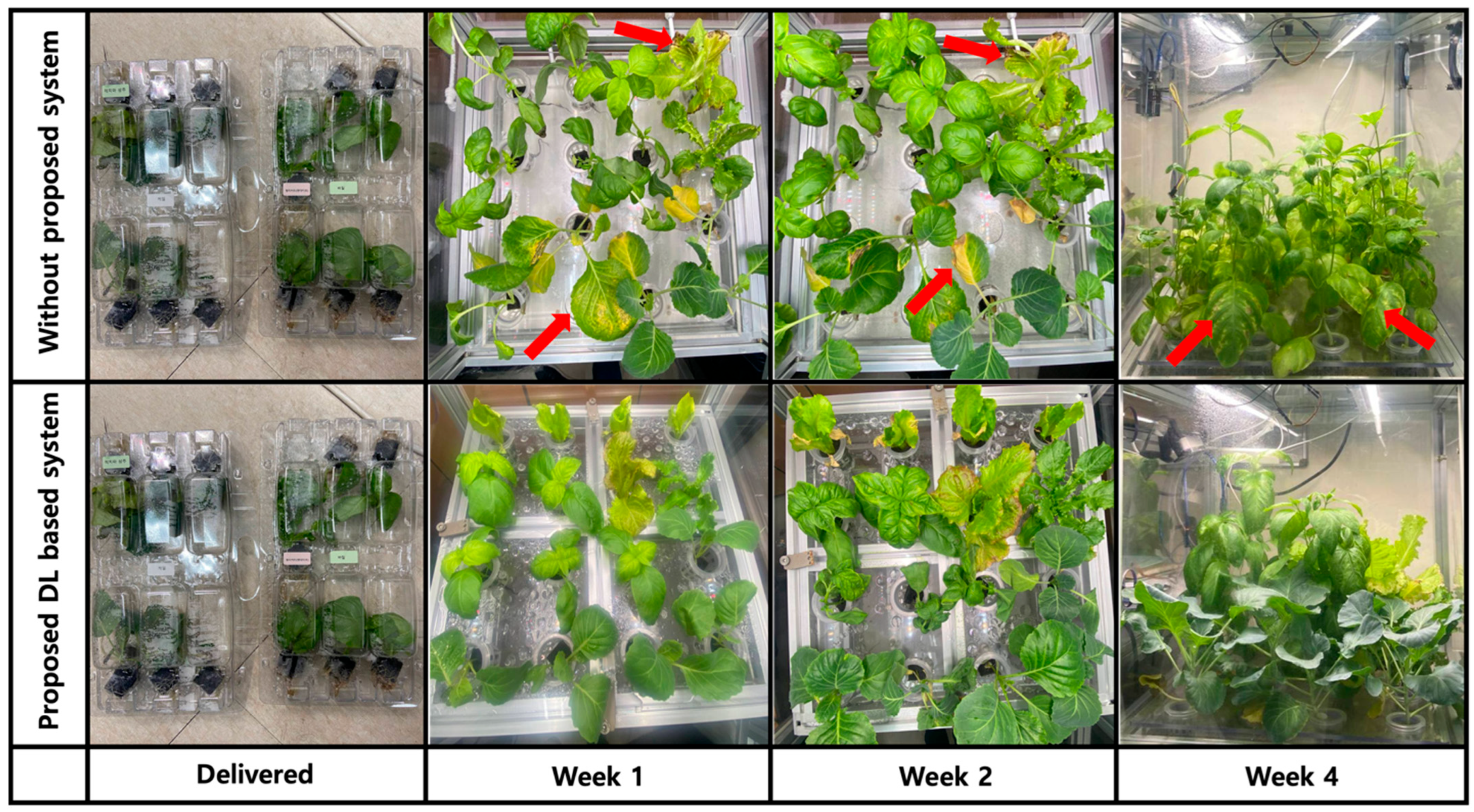
The impact on crop productivity is substantial. The DL-based system’s predictive capabilities and adaptive control contribute to enhanced productivity as plants experience consistent and optimized growth environments. In a contrasting scenario, traditional greenhouse setups, lacking sophisticated control mechanisms, may witness fluctuations in environmental conditions, potentially hindering crop yields. Operational efficiency is another dimension where the DL-based system shines. Automation and intelligence reduce the need for constant manual oversight, contributing to increased operational efficiency. In contrast, traditional greenhouse management demands more manual intervention, potentially resulting in delays in responding to environmental changes and addressing issues promptly. From an environmental perspective, the DL-based control system aligns with sustainability goals. Precise control and optimization translate to reduced resource wastage, fostering eco-friendly agricultural practices. In contrast, traditional greenhouse models, with their inherent inefficiencies, may contribute to higher resource consumption and a larger environmental footprint. In essence, the adoption of a DL-based control system in the smart greenhouse environment marks a paradigm shift. The transformative impact across climate regulation, resource utilization, crop productivity, operational efficiency, and environmental sustainability underscores the potential of advanced technologies in shaping the future of agriculture. Numerous experimental trials were conducted within the framework of the envisioned smart indoor hydroponic greenhouse. A comprehensive assessment was undertaken by cultivating four distinct plant varieties during a specific experiment. The climatic conditions for this experiment were meticulously controlled, with the temperature, humidity, and CO₂ levels set at 23 °C, 65%, and 450 ppm, respectively (refer to Figure 9). In parallel, an identical experiment was conducted without the integration of our proposed system. The outcomes of these comparative experiments are presented in Figure 10. The results highlight potential plant health issues in the absence of the proposed system, evident in the form of yellowish discolorations on the leaves. These anomalies are attributed to unfavorable climate parameters, including elevated humidity, increased temperature, or decreased CO₂ levels. Conversely, the plants cultivated within the smart greenhouse equipped with our proposed system exhibit a healthier state.

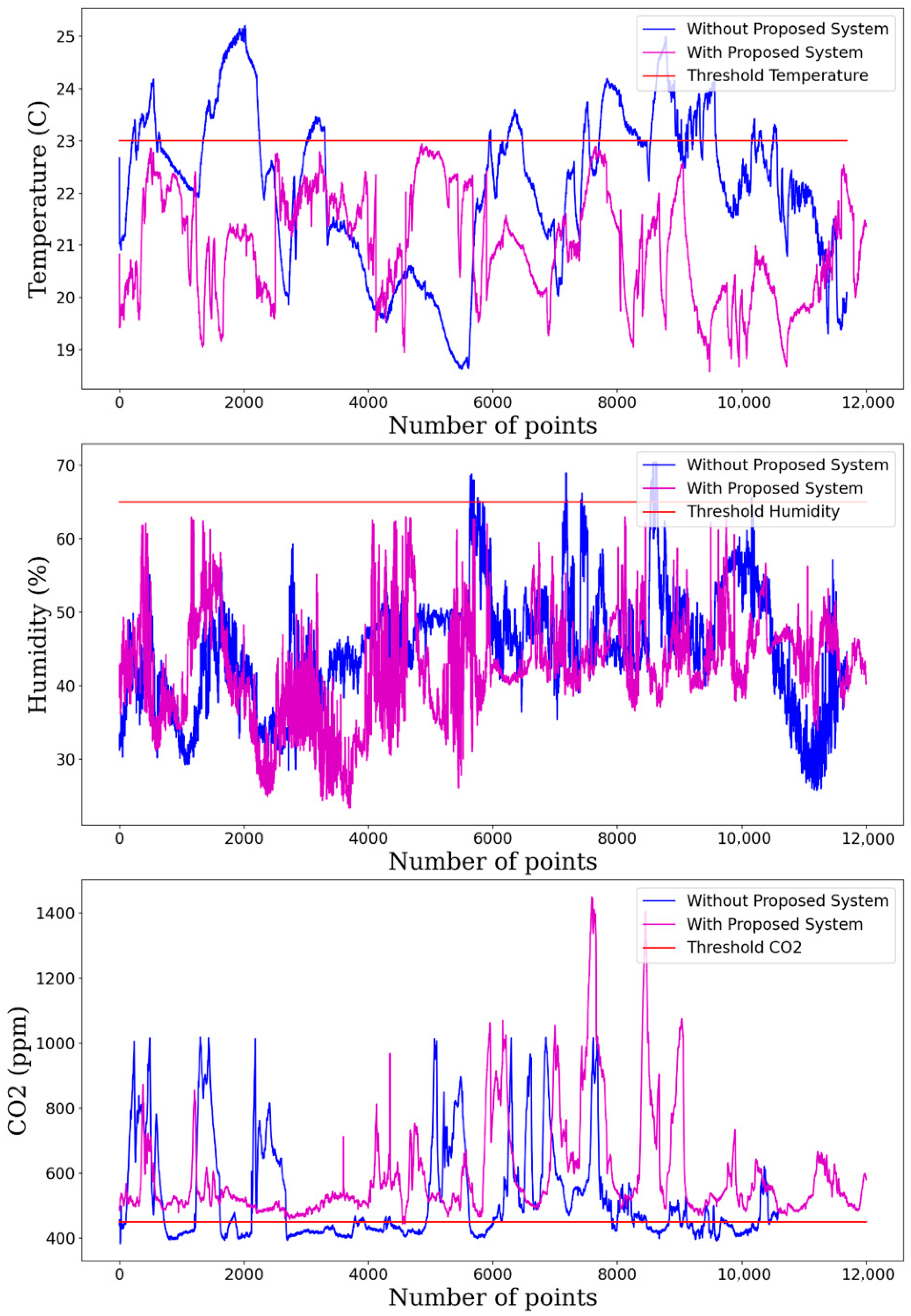
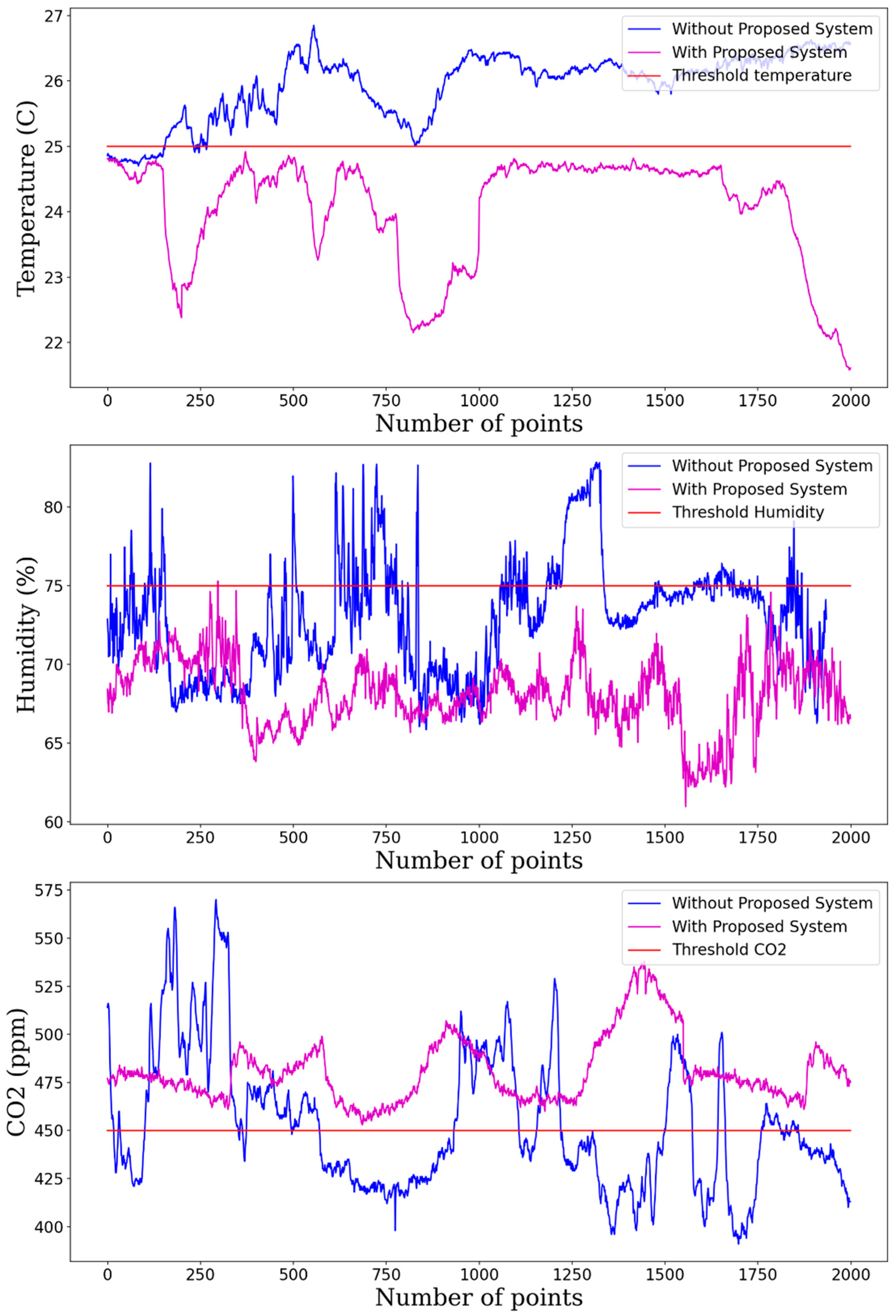
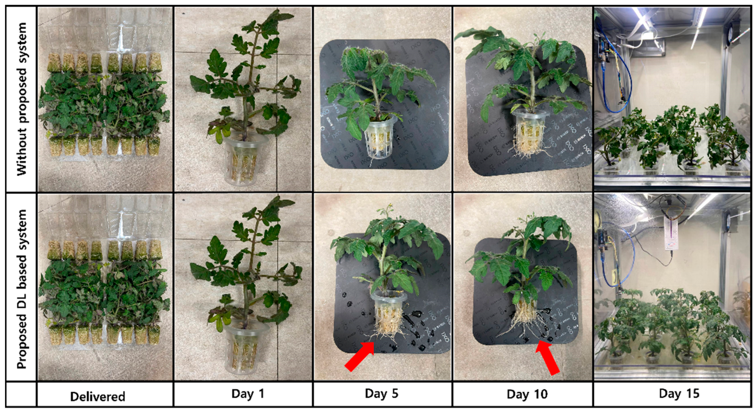
Furthermore, specific experimentation involving the cultivation of tomato plants was undertaken. Illustrated in Figure 11, the tomato plants within our smart greenhouse exhibited accelerated growth compared to those in a conventional hydroponic smart greenhouse. This disparity in growth rates is attributed to the substantially longer roots observed in tomato plants cultivated within the smart greenhouse. The controlled parameters for this experiment, encompassing temperature, humidity, and CO₂ levels, were maintained at 25 °C, 75%, and 450 ppm, respectively. Climate parameter measurements from hydroponic smart greenhouses, both with and without our proposed DL-based controlling system, are presented in Figure 12. The experimental findings demonstrate that the climate parameters crucial for optimal plant growth and health consistently fall within the prescribed range when the DL-based autonomous controlling system is employed. In contrast, the absence of the proposed DL-based autonomous controlling system results in fluctuating and unstable climate parameters, potentially compromising the well-being of the cultivated plants within the hydroponic smart greenhouse.

From a hardware standpoint, the proposed system demonstrates high efficiency due to the lightweight 1D-CNN model and the use of the Jetson Nano platform, which offers a balance of computational power and energy efficiency suitable for edge AI applications. However, when considering deployment at a commercial scale, several challenges arise. These include the need for a denser sensor network to cover larger growing areas, increased computational overhead for real-time predictions from multiple zones, and integration difficulties with diverse greenhouse automation systems. Moreover, ensuring consistent wireless connectivity, data integrity, and fault-tolerant operation becomes increasingly important. Addressing these challenges will require further research into distributed model inference, low-power AI hardware, and standardized communication protocols to support reliable large-scale deployment in real-world agricultural environments.

5. Conclusions

In conclusion, our research successfully addresses challenges within indoor cultivation by introducing a novel Deep Learning (DL)-based optimal condition monitoring system. Through the integration of DL models, our system provides real-time predictions and enables adaptive control, overcoming limitations associated with traditional approaches. The comprehensive approach of combining hydroponics with DL-based optimal control demonstrates significant improvements in the efficiency and responsiveness of indoor cultivation systems. The positive outcomes observed in plant growth experiments underscore the practical implications of our research, showcasing the potential for the widespread adoption of advanced technologies in greenhouse environments. As technology continues to evolve, our study lays the groundwork for future advancements in sustainable and automated indoor farming practices, contributing to the broader discourse on the intersection of agriculture and artificial intelligence.

While the results of this study are promising, it is important to acknowledge a key limitation: the experimental dataset was collected over the relatively short period of one week. This limited time frame may not fully capture seasonal variations, long-term plant growth cycles, or evolving greenhouse dynamics. To ensure the robustness and scalability of the proposed system, future work should involve extended experiments across multiple weeks or months, incorporating different crop types and seasonal conditions. Such long-term testing would provide deeper insights into system adaptability and reliability under varying environmental stressors and further strengthen the case for deploying AI-based symmetry-aware control systems in commercial greenhouse operations.

References

1. Prabhu, B.; Pradeep, M.; Gajendran, E. Monitoring Climatic Conditions Using Wireless Sensor Networks. Available online: https://papers.ssrn.com/sol3/papers.cfm?abstract_id=2905669 (accessed on 1 February 2025).
2. Li, W.; Zheng, T.; Yang, Z.; Li, M.; Sun, C.; Yang, X. Classification and Detection of Insects from Field Images Using Deep Learning for Smart Pest Management: A Systematic Review. Ecol. Inform. 2021, 66, 101460. [Google Scholar] [CrossRef]
3. Zheng, Y.Y.; Kong, J.L.; Jin, X.B.; Wang, X.Y.; Su, T.L.; Zuo, M. Cropdeep: The Crop Vision Dataset for Deep-Learning-Based Classification and Detection in Precision Agriculture. Sensors 2019, 19, 1058. [Google Scholar] [CrossRef]
4. Čirjak, D.; Miklečić, I.; Lemić, D.; Kos, T.; Živković, I.P. Automatic Pest Monitoring Systems in Apple Production under Changing Climatic Conditions. Horticulturae 2022, 8, 520. [Google Scholar] [CrossRef]
5. Ojo, M.O.; Zahid, A. Deep Learning in Controlled Environment Agriculture: A Review of Recent Advancements, Challenges and Prospects. Sensors 2022, 22, 7965. [Google Scholar] [CrossRef]
6. Shi, J.; Xie, W.; Huang, X.; Xiao, F.; Usmani, A.S.; Khan, F.; Yin, X.; Chen, G. Real-Time Natural Gas Release Forecasting by Using Physics-Guided Deep Learning Probability Model. J. Clean. Prod. 2022, 368, 133201. [Google Scholar] [CrossRef]
7. Jung, D.H.; Kim, H.S.; Jhin, C.; Kim, H.J.; Park, S.H. Time-Serial Analysis of Deep Neural Network Models for Prediction of Climatic Conditions inside a Greenhouse. Comput. Electron. Agric. 2020, 173, 105402. [Google Scholar] [CrossRef]
8. van Mourik, S.; van Beveren, P.J.M.; López-Cruz, I.L.; van Henten, E.J. Improving Climate Monitoring in Greenhouse Cultivation via Model Based Filtering. Biosyst. Eng. 2019, 181, 40–51. [Google Scholar] [CrossRef]
9. Weldeslasie, D.T.; Assres, G.; Grønli, T.M.; Ghinea, G. Automated Climate Monitoring System: The Case of Greenhouse Industries in Ethiopia. Internet Things 2021, 15, 100426. [Google Scholar] [CrossRef]
10. Gong, L.; Yu, M.; Jiang, S.; Cutsuridis, V.; Pearson, S. Deep Learning Based Prediction on Greenhouse Crop Yield Combined TCN and RNN. Sensors 2021, 21, 4537. [Google Scholar] [CrossRef] [PubMed]
11. Ferentinos, K.P.; Katsoulas, N.; Tzounis, A.; Bartzanas, T.; Kittas, C. Wireless Sensor Networks for Greenhouse Climate and Plant Condition Assessment. Biosyst. Eng. 2017, 153, 70–81. [Google Scholar] [CrossRef]
12. Ullah, I.; Fayaz, M.; Aman, M.; Kim, D. Toward Autonomous Farming—A Novel Scheme Based on Learning to Prediction and Optimization for Smart Greenhouse Environment Control. IEEE Internet Things J. 2022, 9, 25300–25323. [Google Scholar] [CrossRef]
13. Siddiqui, M.F.; Ur Rehman Khan, A.; Kanwal, N.; Mehdi, H.; Noor, A.; Khan, M.A. Automation and Monitoring of Greenhouse. In Proceedings of the 2017 International Conference on Information and Communication Technologies ICICT, Karachi, Pakistan, 30–31 December 2017; pp. 197–201. [Google Scholar] [CrossRef]
14. Mehra, M.; Saxena, S.; Sankaranarayanan, S.; Tom, R.J.; Veeramanikandan, M. IoT Based Hydroponics System Using Deep Neural Networks. Comput. Electron. Agric. 2018, 155, 473–486. [Google Scholar] [CrossRef]
15. Lee, J.; Im, S.; Jeong, J.S.; Lee, T.S.; Park, S.H.; Shin, C.; Ju, H.; Kim, H.J. Learning Hidden Relationship between Environment and Control Variables for Direct Control of Automated Greenhouse Using Transformer-Based Model. Comput. Electron. Agric. 2025, 235, 110335. [Google Scholar] [CrossRef]
16. Lee, M.H.; Yao, M.H.; Kow, P.Y.; Kuo, B.J.; Chang, F.J. An Artificial Intelligence-Powered Environmental Control System for Resilient and Efficient Greenhouse Farming. Sustainability 2024, 16, 10958. [Google Scholar] [CrossRef]
17. Ait Oussous, S.; Lail, D.M.; El Bouayadi, R.; Amine, A. Deep Learning Innovations for Greenhouse Climate Prediction: Insights from a Spanish Case Study. IEEE Access 2025, 13, 64810–64821. [Google Scholar] [CrossRef]
18. Eraliev, O.; Lee, C.-H. Performance Analysis of Time Series Deep Learning Models for Climate Prediction in Indoor Hydroponic Greenhouses at Different Time Intervals. Plants 2023, 12, 2316. [Google Scholar] [CrossRef] [PubMed]
19. Ugli, O.E.M.; Lee, K.H.; Lee, C.H. Automatic Optimization of One-Dimensional CNN Architecture for Fault Diagnosis of a Hydraulic Piston Pump Using Genetic Algorithm. IEEE Access 2023, 11, 68462–68472. [Google Scholar] [CrossRef]
20. Kamilaris, A.; Prenafeta-Boldú, F.X. Deep Learning in Agriculture: A Survey. Comput. Electron. Agric. 2018, 147, 70–90. [Google Scholar] [CrossRef]
21. Nury, A.H.; Hasan, K.; Alam, M.J. Bin Comparative Study of Wavelet-ARIMA and Wavelet-ANN Models for Temperature Time Series Data in Northeastern Bangladesh. J. King Saud Univ. Sci. 2017, 29, 47–61. [Google Scholar] [CrossRef]
22. Moon, T.; Ahn, T.I.; Son, J.E. Forecasting Root-Zone Electrical Conductivity of Nutrient Solutions in Closed-Loop Soilless Cultures via a Recurrent Neural Network Using Environmental and Cultivation Information. Front. Plant Sci. 2018, 9, 328105. [Google Scholar] [CrossRef] [PubMed]
Figure 1. A graphical representation of directly connected two convolutional layers.
Symmetry 17 01092 g001
Figure 2. Depth-wise dimension reduction based on 1 × 1 convolutions.
Symmetry 17 01092 g002
Figure 3. The proposed DL model: (a) 1D-CNN block, (b) overall network architecture.
Symmetry 17 01092 g003
Figure 4. Overall flowchart of the controlling system of the smart greenhouse.
Symmetry 17 01092 g004
Figure 5. Prototype of IoT- and AI-based autonomous hydroponic smart greenhouse.
Symmetry 17 01092 g005
Figure 6. Temperature prediction results using the DL models per time step: (a) 1 min time step, (b) 5 min time step, (c) 10 min time step, (d) 15 min time step.
Symmetry 17 01092 g006
Figure 7. Humidity prediction results using DL models per time step: (a) 1 min time step, (b) 5 min time step, (c) 10 min time step, (d) 15 min time step.
Symmetry 17 01092 g007
Figure 8. CO2 prediction results using DL models per time step, (a) 1 min time step, (b) 5 min time step, (c) 10 min time step, (d) 15 min time step.
Symmetry 17 01092 g008
Figure 9. Comparison of climate parameters of smart greenhouse with the proposed system and without the proposed system.
Symmetry 17 01092 g009
Figure 10. Comparison of plant conditions in the smart greenhouse with and without the proposed system. The red arrow highlights signs of yellowing and poor leaf health observed in plants grown without environmental symmetry control.
Symmetry 17 01092 g010
Figure 11. Comparison of climate parameters of smart the greenhouse with the proposed system and without the proposed system for tomato plants.
Symmetry 17 01092 g011
Figure 12. Comparison of tomato plant growth conditions in smart greenhouses with and without the proposed system. The red arrow indicates stunted growth in plants exposed to uncontrolled climate fluctuations.
Symmetry 17 01092 g012