Query-Efficient Two-Phase Reinforcement Learning Framework for Black-Box Adversarial Attacks

Abstract

Generating adversarial examples under black-box settings poses significant challenges due to the inaccessibility of internal model information. This complexity is further exacerbated when attempting to achieve a balance between the attack success rate and perceptual quality. In this paper, we propose QTRL, a query-efficient two-phase reinforcement learning framework for generating high-quality black-box adversarial examples. Unlike existing approaches that treat adversarial generation as a single-step optimization problem, QTRL introduces a progressive two-phase learning strategy. The initial phase focuses on training the agent to develop effective adversarial strategies, while the second phase refines the perturbations to improve visual quality without sacrificing attack performance. To compensate for the unavailability of gradient information inherent in black-box settings, QTRL designs distinct reward functions for the two phases: the first prioritizes attack success, whereas the second incorporates perceptual similarity metrics to guide refinement. Furthermore, a hard sample mining mechanism is introduced to revisit previously failed attacks, significantly enhancing the robustness and generalization capabilities of the learned policy. Experimental results on the MNIST and CIFAR-10 datasets demonstrate that QTRL achieves attack success rates comparable to those of state-of-the-art methods while substantially reducing query overhead, offering a practical and extensible solution for adversarial research in black-box scenarios.

1. Introduction

In recent years, growing concerns have emerged regarding the susceptibility of deep neural networks (DNNs) to adversarial examples, especially in high-stakes applications such as facial recognition, autonomous vehicles, and medical diagnostics [1,2]. Adversarial examples are synthesized by applying minimal perturbations to input data, which remain imperceptible to humans, yet can induce machine learning models to generate erroneous predictions with high confidence. As deep learning technologies become increasingly pervasive, their associated security risks have also become more pronounced [3,4].

In the context of understanding the robustness of DNNs, several studies have proposed analyzing this issue from the perspective of symmetry [5,6]. For example, in image recognition tasks, certain geometric transformations of the input (such as rotation and translation) should not affect the semantic content of the model’s predictions. Therefore, the robustness of a model can, to some extent, be interpreted as a manifestation of invariance to such natural symmetries. In contrast, although adversarial perturbations are typically small and imperceptible at the pixel level, they do not correspond to natural symmetry transformations. Rather, they are deliberately crafted inputs designed to disrupt the model’s normal behavior. As a result, the vulnerability of the model to adversarial perturbations reflects a different type of potential generalization issue. These perturbations highlight the model’s vulnerability to inputs that violate natural symmetries. This vulnerability has become an important entry point for research on improving the robustness of DNNs.

Early research focused on white-box attacks [7], in which adversaries possess complete knowledge of the model architecture and gradients, allowing them to craft adversarial inputs through precise manipulation. However, in practical deployment scenarios, the more realistic and prevalent setting is the black-box model, wherein the internal architecture and gradient information of the target model are unavailable. In this context, increasing attention has been directed toward black-box attack methods that rely solely on the model’s output information, such as predicted labels or probability distributions.

Despite their practical significance, current black-box attack techniques encounter two major challenges. First, they typically require numerous queries to the target model, which complicates their deployment in resource-limited environments [8]. Second, the perceptual quality of adversarial examples requires enhancement. In other words, although these examples can induce misclassification, the resulting images frequently exhibit unnatural textures or visible perturbations, rendering them easily detectable by human observers or automated defense mechanisms. Therefore, simultaneously achieving high attack success rates (ASRs) and strict imperceptibility under black-box settings remains an open research challenge.

In response to the aforementioned challenges, this paper proposes a novel black-box adversarial attack framework based on a two-phase reinforcement learning paradigm, termed QTRL. The framework introduces a task-specific dual-phase learning strategy tailored for black-box settings. Unlike existing methods that attempt to simultaneously optimize both the attack success rate and perceptual imperceptibility (PI) within a single learning process, QTRL decouples these inherently conflicting objectives into two separate and progressive training phases. This design is inspired by the principle of curriculum learning, which advocates beginning with simpler tasks and progressively advancing to more complex objectives to facilitate more effective model training.

In the first phase, a reinforcement learning (RL) agent is trained with feedback solely guided by attack success. This phase is designed to efficiently drive the agent to explore and learn perturbation strategies capable of inducing misclassification in the target model, without being constrained by perceptual quality considerations. By focusing exclusively on enhancing attack effectiveness, the agent is able to develop more robust and generalizable strategies across diverse input samples.

In the second phase, a perceptual-quality-oriented optimization mechanism is introduced. While maintaining a high ASR, this phase guides the agent to generate perturbations with greater visual naturalness, thereby enhancing the imperceptibility of adversarial examples. As a fine-grained extension of the first phase, this stage significantly improves the visual stealth of the generated samples, making them not only effective in deceiving the target model but more difficult to detect by human observers or automated defense mechanisms.

To further enhance the robustness and training efficiency of the model, QTRL incorporates a hard sample mining mechanism. During training, all unsuccessfully attacked samples are stored in a dynamic buffer and periodically resampled in subsequent iterations. This “hard sample replay” strategy encourages the agent to continuously learn from its failures, reducing over-reliance on easily attacked samples and thereby improving both the generalization capability and convergence speed of the learned policy.

The main contributions of this paper are summarized as follows:

(1)

We propose an RL-based framework, QTRL, for black-box adversarial attacks. By designing a two-phase curriculum learning strategy, QTRL effectively decouples and optimizes the inherently conflicting objectives of attack success and perceptual quality.

(2)

A hard sample mining mechanism is introduced, which dynamically revisits previously failed attack samples, significantly enhancing the generalization capability of the learned policy.

(3)

Comprehensive evaluations across diverse benchmark datasets and model architectures indicate that QTRL achieves comparable attack success rates to existing methods, while preserving high perceptual quality of adversarial examples and substantially reducing the number of queries. These results validate the practicality and efficiency of QTRL in black-box adversarial attack scenarios.

2. Related Works

2.1. Adversarial Examples

Szegedy et al. [9] initially demonstrated that deep neural networks are vulnerable to adversarial inputs, where imperceptible perturbations $\delta$ deliberately added to an original image x can lead the model to produce highly confident but incorrect predictions. The resulting perturbed instance, denoted as $\widehat{x}=x+\delta$, is referred to as an adversarial example. In recent years, adversarial examples have made significant strides in research within academia. In white-box attacks, the development of adversarial examples has evolved into a comprehensive theoretical framework and methodological approach. These theories and methods can be primarily classified according to their generation mechanisms into several principal categories: the direct optimization of the objective function [9,10], gradient-based attacks [11,12,13,14], decision boundary-based attacks [15,16], and generative neural networks-based attacks [17,18,19]. Each of these methods has demonstrated effective attack outcomes, thereby offering a significant theoretical and practical foundation for the investigation of vulnerabilities and security in deep learning models.

2.2. Black-Box Attacks

Black-box attacks involve generating adversarial examples from a model’s outputs without access to its internal structure or parameters. These attacks are primarily classified into transfer-based attacks and query-based attacks. The former refers to the generation of adversarial examples on a source model, which retain their efficacy when applied to a target model. Nonetheless, variations in model architecture can result in instability in attack success rates (ASRs) [20,21]. Additionally, the lack of dynamic adjustment capabilities makes them susceptible to certain defense mechanisms [22,23].

Recent studies on query-based attacks have concentrated on enhancing query efficiency. Techniques such as LeBA [24], Meta Attack [25], and Simulator Attack [26] have been developed to optimize query efficiency, yielding substantial advancements in attack outcomes. Consistent with this research trajectory, numerous novel attack methodologies have been introduced, including CISA [27], Sparse-rs [28], BBA [29], SparseEvo [30], and NP-attack [31], each demonstrating notable improvements in query efficiency. However, the adversarial examples produced by these techniques frequently exhibit substantial perturbations, thereby compromising the natural appearance of the samples. Current methodologies often face challenges in achieving an optimal balance among three critical metrics: ASR, query count, and extent of image distortion. In response, adversarial attacks have increasingly incorporated deep learning algorithms, such as generative adversarial networks and deep reinforcement learning (DRL) to enhance attack effectiveness.

2.3. RL-Based Black-Box Attacks

Reinforcement learning, renowned for its autonomous learning and decision-making capabilities in complex environments [32,33,34], introduces novel opportunities and challenges for advancing both the theoretical and practical aspects of adversarial attacks. Techniques such as DBAR [35] and RLAB [36] employ reinforcement learning to identify optimal perturbation distributions within the pixel space, thereby facilitating efficient attacks on black-box models. Nonetheless, these methodologies frequently overlook the comprehensive semantic information inherent in images, leading to adversarial examples that appear unnatural. Kang et al. [37] utilized a variational autoencoder to encode images into a latent space, facilitating the efficient generation of more natural adversarial examples within this space through the application of the actor–critic algorithm. Building upon this work, Yu et al. [38] proposed the advRL-GAN framework, which incorporates a feature extractor to derive latent features from images, integrating reinforcement learning and generative adversarial networks to enhance attack effectiveness. Unlike existing methods that attempt to simultaneously optimize both the effectiveness and naturalness of adversarial examples in a single learning process, this paper proposes an RL-based approach to decouple these two conflicting objectives into two distinct and progressive training phases. This approach effectively alleviates the ’balance dilemma’ inherent in traditional methods, ensuring an optimal trade-off between ASR and PI.

3. Proposed Method

This section systematically presents the overall architecture and learning strategy of QTRL (query-efficient two-phase reinforcement learning framework). The architecture of QTRL is illustrated in Figure 1. The method comprises four key modules: (1) a feature space encoder for constructing state representations; (2) a reinforcement learning–based attack environment composed of a decoder and the target model; (3) a two-phase reward function design that decouples attack effectiveness from imperceptibility; and (4) a hard sample mining mechanism aimed at improving attack robustness and accelerate convergence.

3.1. Formal Description

This section focuses on score-based query black-box attacks. Specifically, given a clean input sample $x\in {\mathbb{R}}^d$ and a classifier $f:{\mathbb{R}}^d\to {\mathbb{R}}^c$ that outputs class probabilities over C classes, the predicted label is given as

$$y=argmaxf\left(x\right)=argmax\left[p_0,p_1,\cdots ,p_{C-1}\right].$$

(1)

An adversarial example $\widehat{x}$ is crafted by applying a small perturbation $\delta$ to the original input x, defined as

$$\widehat{x}=x+\delta ,{\parallel \delta \parallel }_p\le \epsilon ,$$

(2)

where $\epsilon$ is the upper bound of the perturbation magnitude, and ${\parallel ·\parallel }_p$ denotes the $l_p$ norm.

In untargeted attacks, the success condition is represented by Equation (3):

$$argmaxf\left(\widehat{x}\right)\ne y,{\parallel \widehat{x}-x\parallel }_p\le \epsilon ,$$

(3)

where y denotes the ground-truth (GT) label.

In targeted attacks, the objective is to generate an adversarial example $\widehat{x}$ such that the target model classifies it into a specific target label $\tau$, i.e.,

$$argmaxf\left(\widehat{x}\right)=\tau \ne y,{\parallel \widehat{x}-x\parallel }_p\le \epsilon .$$

(4)

Building on the above problem formulation, this paper reformulates the score-based black-box attack task as a sequential decision-making problem and introduces a DRL framework to learn attack policies that are both effective and generalizable. In contrast to existing RL-based approaches, we propose a two-phase training strategy: the agent is first trained with a focus on attack effectiveness, and subsequently fine-tuned to improve imperceptibility, thereby maintaining high attack performance while minimizing the visual distortion of adversarial examples.

Specifically, this paper models the attack process as a Markov Decision Process (MDP). In QTRL, the agent interacts with the environment by perceiving states, selecting perturbation actions, and receiving reward feedback, thereby dynamically optimizing its attack strategy. The primary objective is to learn an optimal policy ${\pi }_{\theta }$ that maximizes the expected cumulative reward:

$$\underset{\theta }{max}{E}_{{\pi }_{\theta }}\left[\sum _{t=0}^T{\gamma }^{t}r\left(s_t,a_t\right)\right],$$

(5)

where T represents the total number of time steps, $\gamma$ is the discount factor, $s_t$ is the state at time step t, $a_t$ is the action taken, and $r(s_t,a_t)$ is the reward received. At each step t, the agent determines an action $a_t$ based on the current state $s_t$ and obtains a corresponding reward $r(s_t,a_t)$. By adjusting the policy parameters $\theta$, the agent seeks to maximize the total expected reward across the entire decision-making process.

Notably, in this study, the RL agent has no access to the target model’s internal architecture, parameters, or gradient information during either the training or testing phase. Instead, it can only access the model’s outputs through a limited number of queries. This setup strictly adheres to the assumptions that define the black-box attack setting.

3.2. Overview of the Query-Efficient Two-Phase Reinforcement Learning Framework

3.2.1. Motivation for Two-Stage Design

In black-box adversarial attack tasks, there is often a fundamental trade-off between attack effectiveness and the imperceptibility of perturbations. The former typically requires strong perturbations to alter the model’s prediction, whereas the latter demands minimal changes to preserve visual similarity to the original image. This inherent conflict poses a substantial challenge for designing a unified reward function within an RL framework, thereby hindering both policy convergence and the overall stability of the training process.

As illustrated in Figure 2, we plot the dynamic trajectories of the target class prediction probability and the structural similarity index (SSIM) during progressive perturbations applied to various input samples. These two metrics exhibit a clear inverse relationship: as the prediction probability for the target class increases, the SSIM value consistently decreases. This monotonic divergence highlights a fundamental structural conflict between attack success and perceptual similarity, indicating that

$${\displaystyle \frac{d{f}_{target}\left(x+\delta \right)}{d\delta }}>0,{\displaystyle \frac{ds\left(x,x+\delta \right)}{d\delta }}<0,$$

(6)

where x is the original sample, $\delta$ is the adversarial perturbation, $f_{target}\left(·\right)$ denotes the predicted probability of the target category, and $s\left(·,·\right)$ is the structural similarity function. Evidently, the two objective functions exhibit opposing gradient directions, indicating that they guide the optimization process toward different and potentially conflicting, trajectories in the perturbation space. When both objectives are incorporated simultaneously into the reward function of a reinforcement learning framework, we have, for example,

$$R=f_{target}\left(x+\delta \right)-\lambda \left(1-s\left(x,x+\delta \right)\right).$$

(7)

Consequently, the overall gradient of the reward function can be expressed as

$${\nabla }_{\delta }R={\nabla }_{\delta }{f}_{target}\left(x+\delta \right)+\lambda ·{\nabla }_{\delta }s\left(x,x+\delta \right),$$

(8)

where the perturbation ${\delta }^{\left(2\right)}$ is initialized based on ${\delta }^{\left(1\right)}$.

This staged structure enables the policy to focus on attack effectiveness during the initial training phase, thereby avoiding interference caused by conflicting gradients. In the subsequent phase, the optimization process builds upon the adversarial perturbations learned previously and further concentrates on improving the quality of the perturbations. Compared to the direct weighted combination approach employed in single-phase optimization, the proposed method explicitly decouples the optimization objectives at the structural level, which facilitates more stable convergence of the model and enhances the final perturbation quality.

3.2.2. State Generation Based on Autoencoder

Inspired by related methods in other domains [39,40,41], an autoencoder-based latent state representation module is integrated into QTRL to enhance state modeling in high-dimensional observation spaces. This mechanism not only effectively reduces input dimensionality but also improves the generalization capability of the policy in complex input spaces. Specifically, QTRL employs an autoencoder to extract compact, low-dimensional latent representations from input images, which are subsequently used as the state space for the reinforcement learning framework. This latent space captures the essential structural and semantic features of the original inputs, offering a more stable and informative basis for policy learning. As a result, it significantly enhances both training efficiency and robustness. The structure of the autoencoder is illustrated in Figure 3.

The autoencoder consists of two components: an encoder and a decoder. The former transforms input image $x=\left[z_0,z_1,\cdots z_{n-1}\right]$, consisting of n pixel values, into a compact feature vector $v=\left[g_0,g_1,\cdots g_{m-1}\right]$ of dimension m. This encoding process can be formalized as Equation (9):

$$v=e\left(x\right),$$

(9)

where $e\left(·\right)$ denotes the encoder model. The decoder then reconstructs the input by mapping the latent vector v back to a matrix $x^{\prime }$ with the same dimensions as the original input. This process can be formalized as Equation (10):

$$x^{\prime }=d\left(v\right),$$

(10)

where $d\left(·\right)$ denotes the decoder model. The optimization objective of the autoencoder is shown in Equation (11), and the trained encoder can be used for the feature extraction of input images, resulting in a feature vector v that serves as the state representation for subsequent RL.

$$e·d=\underset{e·d}{argmin}L\left(x,d\left(e\left(x\right)\right)\right),$$

(11)

where L denotes the mean squared error loss function.

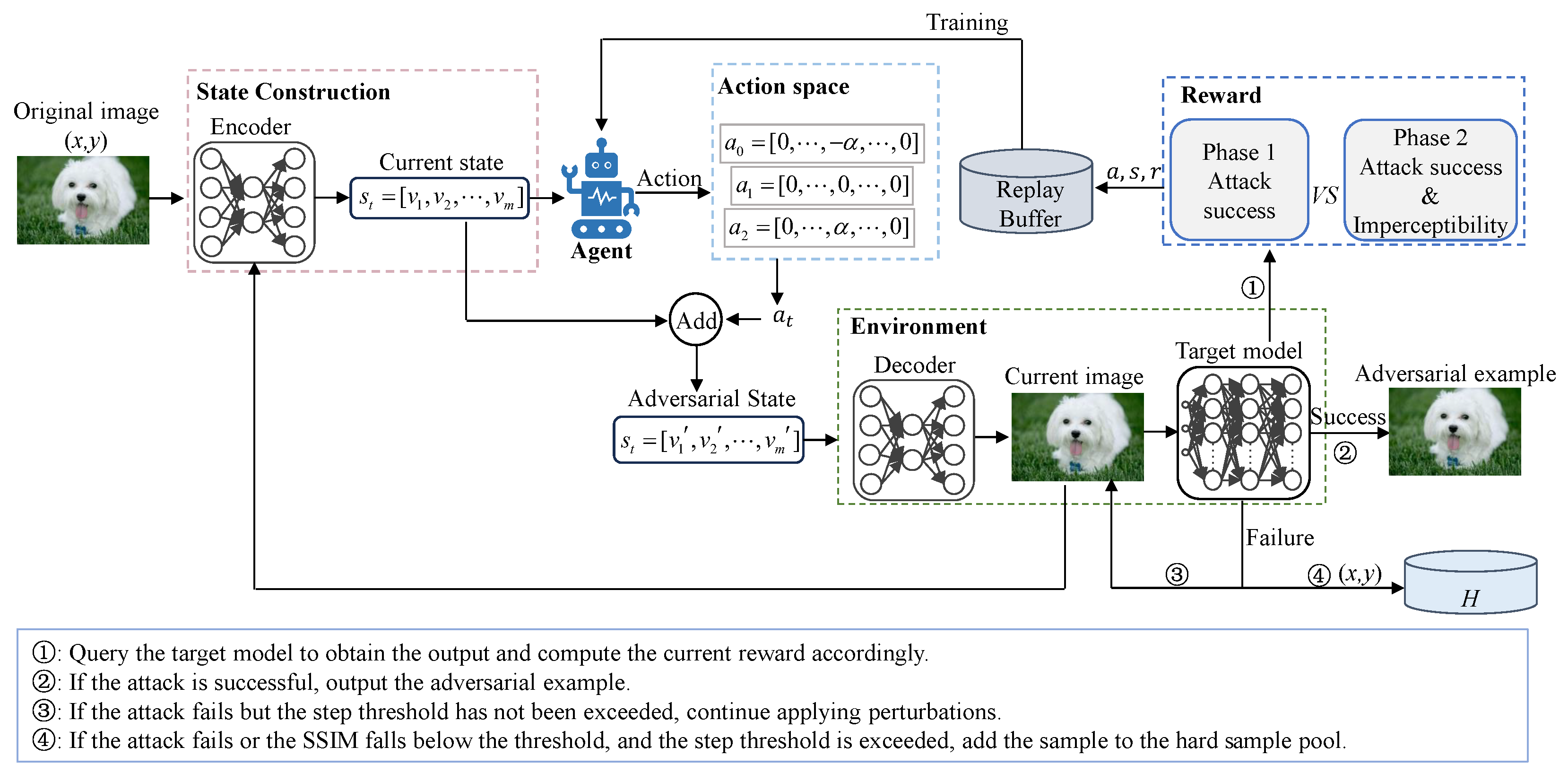
3.2.3. Phase I: Learning to Attack

In the first phase of the proposed framework, the objective is to train an RL agent to acquire effective attack policies that maximize the ASR of adversarial examples. At this phase, the focus is solely on achieving attack success, without regard for perceptual similarity. Specifically, the agent incrementally explores and optimizes action strategies through the RL mechanism to induce incorrect predictions from the target model. The core components of the RL formulation used in this phase are summarized in

Table 1. Design of key elements in the RL framework.

RL Term	Definition in QTRL
Environment	Target model f
State space	Initial state space $S={\left\{v_i\right\}}_{i=1}^N$, where $v_i=\left[g_{i1},g_{i2},\cdots ,g_{im}\right]$
Action space	$A=\left\{a_1,a_2,\cdots ,a_{3m}\right\}$
Policy	$\epsilon$-greedy policy

.

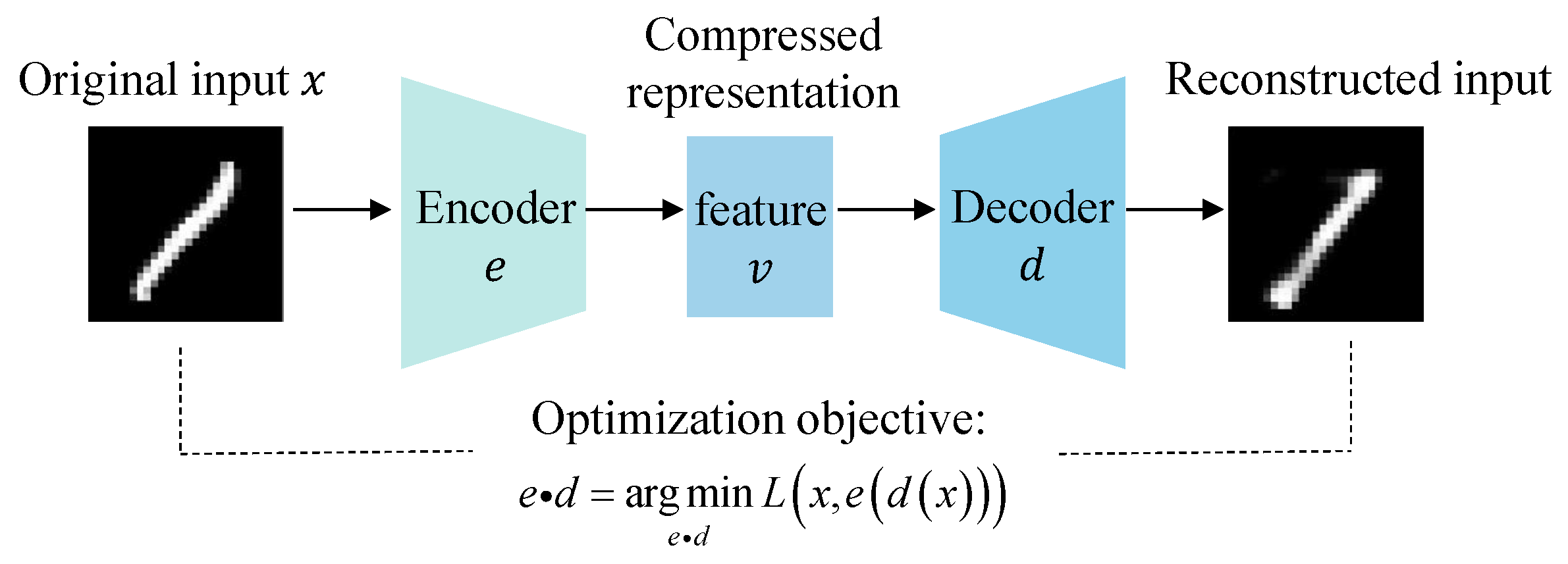
Environment. In QTRL, the environment is composed of a decoder d and a target model f. The decoder reconstructs the latent representations from the feature space into the pixel space, whereas the target model receives the generated adversarial examples and performs classification or prediction.

Action space. The action space is defined as $A=\left\{a_1,a_2,\cdots ,a_{3m}\right\}$, where each action represents a perturbation applied to the input image. Specifically, each action is a sparse vector with the same dimensionality as the feature vector v, perturbing only a single dimension with a fixed magnitude. This design simulates fine-grained adjustments to the input representation. For each dimension, three types of operations are considered: $+\alpha$, 0, and $-\alpha$. The action set is formally expressed as

$$\begin{array}{cc}\hfill {\alpha }_j^{+}& =\left[0,\cdots ,+\alpha ,\cdots ,0\right],j=1,2,\cdots ,m,\hfill \\ \hfill {\alpha }_j^0& =\left[0,\cdots ,0,\cdots ,0\right],j=1,2,\cdots ,m,\hfill \\ \hfill {\alpha }_j^{-}& =\left[0,\cdots ,-\alpha ,\cdots ,0\right],j=1,2,\cdots ,m.\hfill \end{array}$$

(12)

Each vector applies the corresponding perturbation to the j-th dimension while leaving all other elements unchanged. The complete action space can thus be written as $A=\left\{{\alpha }_j^{+},{\alpha }_j^0,{\alpha }_j^{-}\mid j=1,2,\cdots ,m\right\}$.

Given the discrete nature of the action space in this study, Q-learning algorithms demonstrate significant adaptability and advantages for such tasks. By directly learning the state-action value function, Q-learning avoids the need for the explicit modeling of the policy distribution, resulting in more stable training and faster convergence when dealing with high-dimensional yet structurally well-defined discrete action spaces. Moreover, Q-learning can utilize past experiences more efficiently, thereby enhancing data efficiency, which is particularly important in black-box attack scenarios with limited query budgets. Considering both the characteristics of the task and the need for training stability, this study selected the Double Deep Q-Network (DDQN) as the foundational reinforcement learning algorithm.

State space. The initial state space is defined as $S={\left\{v_i\right\}}_{i=1}^N$, where $v_i=\left[e_{i1},e_{i2},\cdots ,e_{im}\right]$, and N represents the number of images. As actions are performed, the dimensionality of the state space gradually increases.

Policy. The agent follows an $\epsilon$-greedy policy, selecting actions based on the exploration-exploitation trade-off.

Reward function design. In contrast to traditional gradient-based methods, our agent operates in the latent feature space, which is derived from a pre-trained autoencoder. Each action taken by the agent results in a small transformation within this latent space, which is then decoded back into the pixel space to generate a perturbed image. The reward function is designed to incentivize the agent to increase the confidence in non-ground-truth classes. A significant reward is given when the prediction shifts away from the original label. In the first phase, QTRL adopts a success-oriented reward function:

$$r_t=\underset{shapingreward}{\underbrace{{\eta }_1·{\Delta }_t}}+\underset{attacksuccess}{\underbrace{{\eta }_2·{\mathbb{I}}_{\mathrm{success}}}},$$

(13)

where ${\eta }_1$ and ${\eta }_2$ are weighting coefficients. Let $p_t$ denote the maximum probability among all non-ground-truth classes predicted by the target model f for the current sample $x_t$ at state $s_t$, and let $\tilde{p}$ represent the highest such probability observed across all previous samples during the agent’s trajectory. Then, ${\Delta }_t$ is defined as

$${\Delta }_t=p_t-\tilde{p},$$

(14)

and ${\mathbb{I}}_{success}$ denotes whether the attack succeeds:

$${\mathbb{I}}_{\mathrm{success}}=\left\{\begin{array}{cc}1,\hfill & \mathrm{if}{p}_t>p_0\hfill \\ 0,\hfill & \mathrm{if}{p}_t\le p_0\hfill \end{array}\right.,$$

(15)

where $p_0$ denotes the predicted probability of the GT by the target model f for the current sample $x_t$ at state $s_t$.

Hard sample mining mechanism. To improve the robustness and generalization ability of the agent, a hard example mining mechanism is introduced in QTRL. The process is illustrated in Figure 4. Specifically, a hard example pool H is constructed to store challenging samples identified during the training process. These hard samples can be categorized into two main types: (1) those for which the attack fails and (2) those for which the attack succeeds but the SSIM between the adversarial and original images falls below a predefined threshold. Such samples are typically more resistant to adversarial perturbations or exhibit greater perceptual differences, thereby posing increased challenges to the attack strategy. By repeatedly training on these hard examples, the agent gains deeper insight into the decision boundaries and perceptual constraints of the target model, ultimately improving both the reliability and stealth of its learned attack policy. The detailed process is outlined in Algorithm 1.

It should be noted that while this mechanism improves the robustness and generalization capability of the policy, it also introduces certain resource overheads. Specifically, during each training iteration, the system must evaluate the performance of training samples under the current policy to select hard samples. Since these hard samples are often reused in subsequent training, a small cache must be maintained in memory. In scenarios involving large-scale datasets or high-resolution images, the high dimensionality and complex distribution of samples can significantly increase the frequency of selection and caching demands, thereby resulting in additional memory and computational burdens. This mechanism can be flexibly adjusted according to specific experimental requirements to balance efficiency and performance.

The proposed hard sample mining mechanism dynamically samples instances that either fail to generate successful adversarial examples or exhibit poor perturbation quality during training, thereby continuously enhancing the agent’s adaptability to boundary cases. This difficulty-driven training signal facilitates the learning of a more discriminative policy function, ultimately improving the model’s generalization capability on out-of-distribution samples. Moreover, hard samples often emerge during training phases where the policy has not yet converged or the model exhibits significant performance fluctuations. Prioritizing such samples in training helps improve the agent’s stability and convergence efficiency when dealing with weak gradient signals or noisy feedback. This mechanism further strengthens the robustness of the policy learning process under conditions of reward bias or noise, contributing to the stability of training in complex or non-ideal environments.

Model training. At each step, the agent selects an action $a_t$ based on policy ${\pi }_{\theta }$ given the current state $s_t$, transitions to the next state $s_{t+1}$, and receives a reward $r_t$ from the environment. The tuple $\left(s_t,a_t,r_t,s_{t+1}\right)$, referred to as a transition sample, is stored in the replay buffer for the subsequent training of the evaluation Q-network. During training, a batch of transitions is randomly sampled from the replay buffer to update the evaluation Q-network. The target value used for this update is computed by the target Q-network, as defined in Equation (16):

$$y_t=r_t+\gamma ·\underset{a\in A}{max}Q\left(s_{t+1},a,{\theta }^{\prime }\right),$$

(16)

where ${\theta }^{\prime }$ denotes the parameters of the target Q-network, and $\gamma \in \left[0,1\right]$ is the discount factor. The loss function used to train the evaluation Q-network is defined as

$$Loss={\displaystyle \frac{1}{2}}{\left[y_t-Q\left(s_t,a_t,\theta \right)\right]}^2.$$

(17)

Algorithm 1: Hard Sample Mining Mechanism.

Input  Phase indicator $phase$, similarity function $s(\widehat{x},x)$, similarity threshold $s_0$, hard pool size threshold $H_0$, policy ${\pi }_{\theta }$  1       Initialize the hard sample pool: $H\leftarrow ⌀$  2       for each episode do:  3         Obtain input sample $(x,y)$  4         while not reached max_step and attack is unsuccessful do:  5           Generate the adversarial example $\widehat{x}$  6           Evaluate attack success and compute the similarity score $s(\widehat{x},x)$  7         if $phase=1$ then:  8           if attack is unsuccessful then:  9             $H.\mathrm{add}(x,y)$  10         end if  11       else:  12         if attack is unsuccessful or $s(\widehat{x},x)<s_0$ then:  13           $H.\mathrm{add}(x,y)$  14         end if  15       end if  16       if $episodemodK=0$ and $\left|H\right|>H_0$ then:  17         Randomly sample a mini-batch $(x_h,y_h)$ from H  18         Perform additional training on $(x_h,y_h)$ to refine the policy ${\pi }_{\theta }$  19       end if  20     end for  Output  Updated agent policy ${\pi }_{\theta }$ with enhanced robustness and generalization

3.2.4. Phase II: Optimizing for Imperceptibility

After the agent has learned to attack successfully, QTRL incorporates visual imperceptibility into the reward function to balance attack effectiveness with perceptual quality. Specifically, the SSIM is adopted as the similarity metric, and the reward function is redesigned as follows:

$$r_t^{\prime }=r_t+\underset{SSIMreward}{\underbrace{{\eta }_3·\varphi \left(s\left(x_0,x_t\right)\right)}}+\underset{SSIMpenalty}{\underbrace{{\eta }_4·{\mathbb{I}}_{penalty}^s}},$$

(18)

where ${\eta }_3$ and ${\eta }_4$ are weighting coefficients, $\varphi \left(·\right)$ is defined as

$$\varphi \left(s\left(x_0,x_t\right)\right)=max\left(0,min\left({\eta }_5·\left(s\left(x_0,x_t\right)-s_0\right),1\right)\right),$$

(19)

and ${\mathbb{I}}_{penalty}^s$ is defined as

$${\mathbb{I}}_{\mathrm{penalty}}^s=\left\{\begin{array}{cc}-k,\hfill & \mathrm{if}s(x_0,x_t)<s_1\hfill \\ 0,\hfill & \mathrm{otherwise}\hfill \end{array}\right.,$$

(20)

where $s_0$ and $s_1$ are both SSIM threshold values, and $k>0$ denotes a constant..

Equation (18) is designed to motivate the agent to achieve adversarial misclassification while preserving the visual similarity to the original input as much as possible. Phase II training is initiated after a predetermined number of training episodes. Algorithm 2 presents the overall procedure of the proposed two-phase reinforcement learning framework. In each training episode, the agent interacts with the target model in a black-box manner by perturbing the feature representation $v_t$ of the input image. Depending on the current phase, the agent receives the corresponding reward signals: Phase I focuses on improving the attack success rate, while Phase II emphasizes both attack effectiveness and the preservation of perceptual quality. Samples that consistently fail to be perturbed successfully or have an SSIM below the threshold are added to a hard sample pool H for more focused training attention.

Algorithm 2: Two-phase reinforcement learning framework.

Input  Target model f, training dataset $D=\left\{(x,y)\right\}$, encoder e, decoder d, agent policy ${\pi }_{\theta }$, learning rate $\eta$, maximum steps per episode T, total number of episodes N, phase transition threshold $N_t$  1       Initialize the agent parameters $\theta$, replay buffer B, hard sample pool $H\leftarrow ⌀$, historical maximum confidence $c\leftarrow 0$, phase indicator $phase\leftarrow 1$  2       for episode = 1 to N do  3         if $phase=1$ and $episode>N_t$ then  4           $phase\leftarrow 2$  5         end if  6         Sample $(x,y)$ from D or H according to a predefined schedule  7         Encode features: $z_0\leftarrow e\left(x\right)$, initialize the state $s_0\leftarrow z_0$  8         Initialize the confidence tracker $c\leftarrow 0$  9         for $t=0$ to T do  10         Select action $a_t={\pi }_{\theta }\left(s_t\right)$  11         Update state: $s_{t+1}\leftarrow s_t+a_t$, decode $x_{t+1}\leftarrow d\left(s_{t+1}\right)$  12         Query target model: $p\leftarrow f\left(x_{t+1}\right)$, obtain prediction $\widehat{y}$  13         Compute reward: $r_t\leftarrow \mathrm{Reward}(p,y,c,phase)$  14         Store transition $(s_t,a_t,r_t,s_{t+1})$ in buffer B  15         Update policy ${\pi }_{\theta }$ using DDQN with samples from buffer B  16         if attack is successful then  17           break  18         end if  19       end for  20       Add samples to H based on the Algorithm 1  21     end for  Output  Trained agent policy ${\pi }_{\theta }$

By virtue of the QTRL framework’s design principle that effectively decouples attack success from perturbation optimization objectives, the implementation details of the reward functions in both stages demonstrate strong robustness. Specifically, provided that the reward function clearly drives attack success in the first stage and effectively guides perceptual similarity optimization in the second stage, the framework’s core mechanism can operate stably and achieve the intended objectives. Meanwhile, the hard sample mining mechanism, through dynamic identification and training on samples with failed attacks or low-quality perturbations, enhances the agent’s adaptability to boundary samples. This dual mechanism not only reduces reliance on complex reward shaping but improves the method’s practicality and deployability across diverse scenarios.

3.2.5. Attack Cost Modeling and Efficiency Evaluation

To quantitatively evaluate the overall efficiency of the QTRL method in practical black-box attack scenarios, a theoretical model is established to analyze the total cost incurred during the adversarial attack process. The total attack cost associated with QTRL can be divided into two main components: the first is the computational resource overhead required during the training phase, representing the one-time policy learning cost; the second is the query cost generated from interactions with the target model during the attack phase. Specifically, the total attack cost is defined as follows:

$$C_{total}=C_{train}+C_{query}·Q·N,$$

(21)

where $C_{train}$ denotes the fixed computational overhead required for training the RL policy. This is a one-time cost independent of the number of attack samples. $C_{query}$ represents the average cost per query during the attack process. Q is the average number of queries required per attack. N denotes the total number of attack samples.

Although QTRL introduces a fixed training overhead $C_{train}$, it significantly reduces the average number of queries Q required per attack. Consequently, the total cost tends to grow approximately linearly with the number of attack samples. As the attack scale increases, QTRL becomes more cost-efficient compared to strategies that require no training but incur a higher average number of queries per attack.

Furthermore, a cost-equilibrium point $N^{*}$ can be defined as the minimum number of attack samples that satisfies the following condition:

$$C_{train}<C_{query}·\left(Q_{baseline}-Q_{QTRL}\right)·N\Rightarrow N^{*}={\displaystyle \frac{C_{train}}{C_{query}·\left(Q_{baseline}-Q_{QTRL}\right)}},$$

(22)

where $Q_{baseline}$ is the reference metric, representing the average number of queries required per attack in the absence of an agent-based training mechanism. When the number of attack samples N exceeds $N^{*}$ (i.e., $N>N^{*}$), the query cost savings achieved by QTRL outweigh its training overhead, thereby demonstrating a significant advantage in overall efficiency.

Therefore, the design of QTRL is well suited for large-scale black-box attack tasks in practical scenarios. In applications involving attacks on multiple target images or the continuous execution of attack strategies, the initial training cost can be rapidly amortized, while the reduced online query overhead significantly improves overall attack efficiency. This cost structure not only ensures the method’s effectiveness but also endows QTRL with strong scalability and practical deployment value.

4. Experiment Results and Analysis

4.1. Experimental Settings

Dataset: This study employed the MNIST [42] and CIFAR-10 [43] datasets to evaluate the effectiveness of the proposed method. Specifically, a random subset of 1000 samples from the MNIST test set was used for evaluation, whereas the full CIFAR-10 test set was employed.

Target Model Architecture: For the MNIST dataset, the target models included ResNet-50 [44] and a custom four-layer convolutional neural network, referred to as Model $\mathcal{A}$. The architecture and training parameters of Model $\mathcal{A}$ are detailed in

Table 2. Architecture and training parameters of the target models on the MNIST dataset.

Architecture			Parameters
			Model $\mathcal{A}$	ResNet-50
Conv.ReLU	$3\times 3\times 32$	Optimization	SGD	Adam
Conv.ReLU	$3\times 3\times 32$	Dropout	0.5	–
Max Pooling	$2\times 2$	Loos function	Cross Entropy	Cross Entropy
Conv.ReLU	$3\times 3\times 64$	Learning rate	0.1	0.001
Conv.ReLU	$3\times 3\times 64$	Bach size	128	128
Max Pooling	$2\times 2$	Momentum	0.9	–
Dense.ReLU	200	Accuracy rate	99.20%	99.16%
Dense.ReLU	200
Softmax	10

. For the CIFAR-10 dataset, ResNet-32 [44] and VGG-19 [45] were selected as target models.

Attack Scenario: The proposed method was evaluated under a score-based black-box attack setting, with a primary focus on untargeted attacks.

Evaluation Metrics: This study employed three evaluation metrics to assess the performance of the proposed method: attack success rate, image quality, and query efficiency:

(1)

Attack Success Rate: The proportion of adversarial examples that successfully cause the target model to make incorrect predictions. A higher success rate indicates a more effective attack.

(2)

Image Quality: This metric measures the visual similarity between adversarial examples and the corresponding original images. In this work, the SSIM was used to quantify the imperceptibility of perturbations.

(3)

Query Efficiency: Following previous studies [25,26,27,28,29,30,31], query efficiency in this paper refers to the number of queries to the target model required to generate an adversarial example. A lower average number of queries indicates a more efficient attack strategy.

4.2. Results of the Autoencoder

For the MNIST dataset, a fully connected autoencoder was implemented, whereas a convolutional autoencoder was employed for the CIFAR-10 dataset. The architectures and corresponding training parameters for both models are summarized in

Table 3. Architecture and training parameters of the autoencoder for the MNIST dataset.

Architecture		Parameters
Dense.ReLU	500	Optimization	Adam
Dense.ReLU	256	Dropout	0.5
Dense.ReLU	64	Loos function	MSE
Dense.ReLU	20	Learning rate	0.0001
Dense.ReLU	64	Bach size	32
Dense.ReLU	256	Loss value	0.017
Dense.ReLU	500
Sigmode	10

and

Table 4. Architecture and training parameters of the autoencoder for the CIFAR-10 dataset.

Architecture		Parameters
Conv.ReLU	4 × 4 × 12	Optimizer	SGD
Conv.ReLU	4 × 4 × 24	Optimizer	Adam
Conv.ReLU	4 × 4 × 48	Learning rate	0.01
Conv.ReLU	4 × 4 × 96	Batch size	16
ConvTranspose2d + ReLU	4 × 4 × 48	Loss value	0.551
ConvTranspose2d + ReLU	4 × 4 × 24
ConvTranspose2d + ReLU	4 × 4 × 12
ConvTranspose2d + ReLU	4 × 4 × 3

, respectively.

Figure 5 presents the image reconstruction results of the autoencoders. The original and reconstructed images from the MNIST dataset are displayed in the first and second rows, respectively, while the third and fourth rows show the corresponding images from the CIFAR-10 dataset. These results demonstrate that the designed autoencoders can effectively extract features from the input images and demonstrate strong reconstruction ability.

4.3. Attack Results

4.3.1. Attack Results of QTRL on Target Models

To thoroughly assess the attack performance of QTRL, score-based black-box attack experiments were performed on the MNIST and CIFAR-10 datasets, with results compared to those of leading attack methods. Considering the instability of reinforcement learning convergence in adversarial attack tasks, separate Q-networks were trained for each target class to accelerate convergence and improve policy stability. During training, a consistent greedy policy and a unified discount factor were used to ensure coherence in the decision-making process. The detailed experimental settings are summarized in

Table 5. Experimental parameter settings.

Parameter	Description	Default Value
		MNIST	CIFAR-10
n	Number of actions	60	1152
m	Dimension of the eigenvector	20	384
$\gamma$	Discount factor	0.99	0.99
h	Updating target Q’s interval	1000	1000
B	Batch size	256	256
${\eta }_1$	Parameters in Equation (10)	0.50	1.00
${\eta }_2$	Parameters in Equation (10)	3.00	3.00 (phase 1)
			5.00 (pahse 2)
${\eta }_3$	Parameters in Equation (15)	1.00	1.00
${\eta }_4$	Parameters in Equation (15)	1.00	1.00
${\eta }_5$	Parameters in Equation (16)	5.00	5.00
$s_0$	Parameters in Equation (16)	0.80	0.95
$s_1$	Parameters in Equation (17)	0.75	0.85

.

Score-based untargeted black-box attack experiments were conducted across all classes of the MNIST and CIFAR-10 datasets. The target models include ResNet-50 and Model A for MNIST and ResNet-32 and VGG-19 for CIFAR-10. The attack performance of QTRL on both datasets is shown in

Table 6. Attack results of QTRL on target models evaluated on the MNIST dataset. (ASR: attack success rate [%]; SSIM: structural similarity index; Avg.Q: average number of queries; Avg.: average value.)

Label	ResNet-50			Model A
	ASR	SSIM	Avg.Q	ASR	SSIM	Avg.Q
0	1.000	0.629	13.63	1.000	0.644	9.34
1	1.000	0.731	16.01	1.000	0.763	10.51
2	1.000	0.574	20.01	1.000	0.654	11.42
3	1.000	0.727	12.56	1.000	0.720	10.08
4	1.000	0.713	12.94	1.000	0.692	11.04
5	1.000	0.644	13.08	1.000	0.607	13.08
6	1.000	0.729	10.12	1.000	0.642	14.25
7	1.000	0.767	10.84	1.000	0.738	10.09
8	1.000	0.767	8.34	1.000	0.710	9.03
9	1.000	0.747	10.43	1.000	0.769	11.08
Avg.	1.000	0.703	12.80	1.000	0.694	10.99

and

Table 7. Attack results of QTRL on target models evaluated on the CIFAR-10 dataset.

Label	ResNet-32						VGG-19
	Phase I			Phase II			Phase I			Phase II
	ASR	SSIM	Avg.Q	ASR	SSIM	Avg.Q	ASR	SSIM	Avg.Q	ASR	SSIM	Avg.Q
0	0.825	0.675	38.55	0.992	0.766	4.66	0.996	0.718	4.07	1.000	0.750	2.50
1	1.000	0.755	5.03	1.000	0.826	2.10	0.999	0.760	3.80	0.991	0.786	4.12
2	1.000	0.763	3.24	1.000	0.791	4.81	0.897	0.770	13.11	1.000	0.785	2.38
3	0.996	0.742	5.21	1.000	0.815	2.11	0.993	0.709	5.48	0.997	0.766	3.25
4	0.999	0.730	2.76	0.982	0.740	5.05	0.998	0.709	3.93	1.000	0.736	2.81
5	0.970	0.625	15.77	0.995	0.660	11.94	0.906	0.608	23.66	0.999	0.660	8.77
6	0.999	0.767	3.44	0.984	0.790	3.54	0.982	0.679	6.48	0.999	0.746	2.54
7	0.922	0.742	13.67	1.000	0.764	3.77	0.993	0.653	11.20	1.000	0.758	3.67
8	0.999	0.711	5.86	1.000	0.742	3.89	1.000	0.546	14.75	1.000	0.726	4.56
9	0.883	0.641	20.61	0.995	0.755	4.66	0.826	0.566	30.95	0.986	0.670	7.94
Avg.	0.959	0.715	11.41	0.995	0.765	4.65	0.959	0.672	11.74	0.997	0.738	4.25

.

Table 6 and Table 7 evaluate the method’s performance from three perspectives: the ASR, SSIM, and average number of queries. The results demonstrate that it achieves 100% ASR across all categories on the MNIST dataset, and average ASRs of 99.5% and 99.7% on the CIFAR-10 dataset, thoroughly validating its robustness and stability across different model architectures.

In terms of image similarity, QTRL achieves an average SSIM of 0.703 and 0.694 on the MNIST dataset for the two target models, respectively, while on the CIFAR-10 dataset, the SSIM values are 0.765 and 0.738. This indicates that the method can effectively preserve the visual naturalness of adversarial samples while maintaining a high ASR. Furthermore, the method requires an average of 12.80 and 12.99 queries for the two target models on the MNIST dataset, and 4.65 and 4.25 queries on the CIFAR-10 dataset, respectively, further demonstrating its excellent query efficiency.

To verify the effectiveness of the proposed two-phase attack design, Table 7 presents the attack results for each phase on the CIFAR-10 dataset using ResNet-32 and VGG-19 models. The results demonstrate that, compared to the first phase, the second phase achieves a significant improvement in image quality (as measured by the SSIM), along with an increase in ASR and a substantial reduction in the average number of queries. These findings provide strong evidence that the proposed two-phase design substantially enhances overall attack performance.

Table 8. Experimental results of different methods attacking ResNet-50 on the MNIST dataset.

Attack Methods	ASR	SSIM
C&W [10]	0.619	0.998
FGSM [11]	0.868	0.397
PGD [13]	1.000	0.440
Deepfool [15]	0.729	0.951
QTRL	1.000	0.703

presents a performance comparison between QTRL and four classical white-box attack methods (FGSM, PGD, DeepFool, and C&W) on the ResNet-50 model. White-box attacks, which have direct access to model gradients, are commonly regarded as strong baselines for evaluating the upper bound of attack performance; therefore, they are included in this study for comparative analysis. The experimental results show that both QTRL and PGD achieve a 100% ASR, significantly outperforming DeepFool and C&W in this regard. Although QTRL’s SSIM is slightly lower than that of DeepFool and C&W, the visual quality of its adversarial examples is noticeably superior to those produced by FGSM and PGD. These findings suggest that QTRL, despite operating in a black-box setting, achieves attack performance comparable to white-box methods while maintaining a favorable balance between effectiveness and perceptual quality.

Table 9. Experimental results of different methods attacking ResNet-32 on the CIFAR-10 dataset.

Attack Methods	ASR	Avg.Q
RLAB [36]	1.000	60
SimBA-DCT [47]	1.000	353
CG-Attack [48]	1.000	81.6
EigenBA [49]	0.990	99
QTRL	0.995	4.65

and

Table 10. Experimental results of different methods attacking VGG-19 on the CIFAR-10 dataset.

Attack Methods	ASR	Avg.Q
SRA-CMA-full [46]	1.000	302
SRA-CMA (ref.R) [46]	1.000	1087
QL-Attack [50]	1.000	586
One-Pixel [51]	0.635	23,810
QTRL	0.997	4.25

present the performances of various untargeted attack methods on the CIFAR-10 dataset for the ResNet-32 and VGG-19 models. The performance results of other methods are sourced from experimental data in references [36,46]. The experimental results indicate that QTRL achieves attack success rates of 0.991 and 0.993 on ResNet-32 and VGG-19, respectively, which are close to the 1.000 attack success rate achieved by methods such as SimBA-DCT, CG-Attack, RLAB, QL-Attack, and SRA-CMA. However, these methods show significant differences in query efficiency, measured by the average number of queries. QTRL consistently demonstrates outstanding query efficiency, with average query counts of 4.70 and 6.03 in Table 9 and Table 10, respectively, outperforming all other methods. While many methods achieve high attack success rates (ASRs), QTRL achieves relatively high success rates (ASRs between 0.991 and 0.993) while significantly reducing the number of required queries. This makes it highly valuable for practical applications. QTRL not only maintains excellent attack performance but also reduces computational costs, making it an efficient solution for real-world adversarial attacks.

To provide a clearer illustration of the untargeted attack process, we randomly selected three images from the CIFAR-10 dataset and recorded as well as visualized the changes in the maximum predicted probability among non-ground-truth classes and the SSIM at each step of perturbation addition. As shown in Figure 6, the figure intuitively demonstrates the impact of progressive perturbations on the model’s classification results and image quality. With the accumulation of perturbations, the maximum predicted probability of non-ground-truth classes exhibits an overall increasing trend, while the structural similarity index gradually decreases. This indicates that the attack effectively steers the model away from correct classification while progressively degrading the structural integrity of the images. Moreover, the selected images cover multiple categories, providing a representative sample that further validates the stability and generalizability of the attack across different inputs.

4.3.2. Transfer Attack Results

To further assess the effectiveness of the proposed method in cross-model attack scenarios, bidirectional transfer attack experiments were conducted on the CIFAR-10 dataset. Specifically, adversarial examples were generated using ResNet-32 and VGG19 as source models and then used to attack the other model (i.e., VGG19 and ResNet-32, respectively). The corresponding results are summarized in

Table 11. Results of transfer attacks evaluated on the CIFAR-10 dataset.

Source Model	Target Model	ASR	SSIM	Avg.Q
VGG-19	ResNet-32	0.993	0.737	6.35
ResNet-32	VGG-19	0.984	0.707	8.01

.

As shown in Table 11, in both transfer attack tasks, the proposed method consistently achieves an ASR exceeding 0.98 and an SSIM above 0.70, regardless of the source model. These results indicate that the generated adversarial examples maintain strong attack effectiveness and high perceptual quality when transferred to heterogeneous target models, demonstrating good transferability and stability. Overall, the findings validate the practicality and generalizability of the proposed method in cross-model adversarial attack scenarios. The generated adversarial examples not only exhibit a high ASR but also preserve visual fidelity, highlighting the potential applicability of the method in real-world black-box attack settings.

4.4. Ablation Study

To systematically evaluate the effectiveness of the two-stage design in the QTRL framework, ablation experiments were conducted on the CIFAR-10 dataset using ResNet-32 as the target model. Specifically, two single-stage variants were constructed, employing the reward functions $r_t$ and $r_t’$ defined in Equations (10) and (15), respectively. Apart from the reward functions, the model architecture remained unchanged, and the hyperparameter settings were kept consistent with those listed in Table 5. The experimental results are summarized in

Table 12. Ablation study comparing single-phase and two-phase designs in the QTRL framework on CIFAR-10.

Label	Sigle-Phase (${\mathit{r}}_{\mathit{t}}$)			Sigle-Phase (${\mathit{r}}_{\mathit{t}}^{\prime }$)			QTRL
	ASR	SSIM	Avg.Q	ASR	SSIM	Avg.Q	ASR	SSIM	Avg.Q
0	0.999	0.757	2.98	0.969	0.750	6.32	0.992	0.767	4.66
1	1.000	0.793	2.51	0.999	0.827	1.98	1.000	0.826	2.10
2	1.000	0.748	4.11	1.000	0.783	1.85	1.000	0.791	4.81
3	1.000	0.815	2.09	0.997	0.772	3.75	1.000	0.815	2.11
4	1.000	0.732	3.12	0.980	0.723	5.18	0.982	0.741	5.05
5	0.933	0.634	16.36	1.000	0.747	5.39	0.995	0.660	11.94
6	0.982	0.758	4.90	0.999	0.755	3.74	0.984	0.790	3.54
7	0.990	0.795	3.35	0.910	0.783	12.42	1.000	0.764	3.77
8	1.000	0.723	4.69	1.000	0.723	4.69	1.000	0.742	3.89
9	0.992	0.700	6.44	0.982	0.714	7.49	0.995	0.755	4.66
Avg.	0.990	0.746	5.06	0.984	0.758	5.28	0.995	0.765	4.65

.

As shown in Table 12, the proposed two-phase training mechanism outperforms the single-phase designs across all evaluated metrics. The two-phase design not only achieves the highest attack success rate but significantly surpasses the two single-phase reward functions. While ensuring a substantial improvement in attack effectiveness, QTRL also attains the best structural similarity index, indicating superior visual quality of the generated adversarial examples. Compared to the single-stage reward functions, the proposed two-stage RL strategy achieves a more balanced trade-off between ASR and image quality, thereby demonstrating the rationality and effectiveness of the design.

5. Discussion

5.1. Explainability Analysis of QTRL

In adversarial learning research, model interpretability is particularly critical, especially in safety-critical application domains such as healthcare and autonomous driving. Although RL-based attack strategies demonstrate strong capabilities in modeling nonlinear decision processes, interpretability remains an indispensable consideration in these high-risk fields. To investigate the behavioral mechanisms of the proposed QTRL method within the latent space and its response characteristics to adversarial perturbations, thereby enhancing the transparency and interpretability of the method, this study employs SHapley Additive exPlanations (SHAP) [52,53] to conduct interpretative analyses on both original and adversarial examples. This approach elucidates the influence of latent variables on model decisions, revealing the role of these variables in the decision-making process and how adversarial perturbations affect these mechanisms.

Figure 7 illustrates the distribution of absolute SHAP values across latent dimensions for the original samples (left) and adversarial samples (right), reflecting the relative importance of different feature dimensions to the model’s predictions. A comparative analysis reveals that adversarial perturbations induce significant changes in the model’s reliance on certain features. In the original samples, latent features $z_4$, $z_{1}3$, and $z_{1}6$ exhibit high importance, indicating their dominant roles in the model’s prediction process. In the adversarial examples, the importance of features $z_4$, $z_{1}3$, and $z_{1}2$ increases, whereas the importance of $z_{1}6$, $z_8$, and $z_2$ decreases markedly. These findings suggest that adversarial perturbations do not simply affect predictions by uniformly amplifying or suppressing certain feature values, but rather reshape the model’s attention patterns toward latent features, thereby altering its original decision basis and leading to misclassification.

Figure 7 shows changes in the feature dependence of the classification model under adversarial perturbations generated by QTRL, revealing the interference mechanism of QTRL from the perspective of the latent space. Leveraging the SHAP interpretability tool, the analysis further uncovers alterations in the dependency on key latent features during the model’s decision-making process induced by QTRL. Nevertheless, interpretability analysis remains an evolving field, with numerous challenges still present in its application to the interpretation of complex model behaviors. Future work will focus on incorporating additional explainability techniques, such as Partial Dependence Analysis (PDA), to achieve a more comprehensive understanding of model behavior.

5.2. Limitations and Improvement Directions of QTRL

The proposed QTRL method integrates a hard sample mining mechanism with a two-phase reinforcement learning strategy, demonstrating notable improvements in attack robustness and generalization capability. However, this approach inevitably introduces additional computational and memory overhead, which may adversely affect training efficiency, particularly when dealing with high-resolution images or large-scale datasets.

In addition, the current performance evaluation primarily relies on two metrics: the average number of queries and the attack success rate. While both are highly representative in the context of black-box attacks, they are insufficient to comprehensively assess the method’s practical applicability and resource demands in real-world deployment scenarios. To enable a more systematic evaluation of the overall performance, future work may incorporate hybrid metrics that integrate accuracy, computational complexity, and stability, thereby providing a more objective and fair assessment of the method’s practical utility.

Another critical challenge lies in the generalization capability. In real-world scenarios, image data often exhibit greater complexity and variability, such as illumination changes, viewpoint shifts, and occlusions. These factors can significantly affect the stability and cross-domain transferability of adversarial example generation models, thereby undermining the overall effectiveness of the attacks.

To address the aforementioned challenges, future work can be optimized in the following directions:

(1)

Adopting a shared-policy training framework: By leveraging multi-task learning or shared-input mechanisms, the generalization ability of the policy can be enhanced, thereby improving model robustness and training efficiency without the need for explicit hard sample selection.

(2)

Constructing a multi-dimensional evaluation framework: A comprehensive performance assessment system should be established, incorporating metrics such as query cost, attack success rate, computational complexity, and stability. This would facilitate the systematic validation of the proposed method under fair and rigorous experimental comparisons.

(3)

Focusing on domain adaptation techniques [54,55]: Future work will focus on further mitigating potential distributional discrepancies between training data and the target deployment environment, as well as conducting systematic evaluations on previously unseen independent datasets and real-world images collected from diverse acquisition scenarios, thereby gaining deeper insights into the model’s performance and robustness in heterogeneous environments.

5.3. Challenges in Real-World Deployment

Despite the promising results achieved by QTRL in controlled experimental environments, its deployment in real-world applications remains non-trivial due to a number of practical challenges. The following discussion outlines and analyzes the major issues involved.

Generalization challenges posed by the complexity of real-world image data. Real-world image data often exhibit greater complexity and diversity, including variations in lighting conditions, viewing angles, and occlusions, which can significantly affect the stability and generalization capability of adversarial example generation models, thereby reducing attack effectiveness. To address this generalization challenge, future research should focus on domain adaptation techniques to mitigate potential distributional discrepancies between training data and target application environments. Furthermore, systematic evaluations should be conducted on independent datasets unseen during training, as well as on real-world images collected from diverse sources, to gain a deeper understanding of the model’s performance and robustness across heterogeneous environments.

Efficiency challenges under stringent real-time requirements. Although the proposed method achieves competitive query efficiency through reinforcement learning strategies, response time remains a critical constraint in systems with strict real-time requirements, such as autonomous driving or financial risk control. Future work should therefore aim to further improve overall attack efficiency or incorporate surrogate models to reduce the number of interactions with the target system.

Robustness issues in the presence of defense mechanisms. In real-world deployment scenarios, systems are typically equipped with various defense mechanisms, such as perturbation detection, input preprocessing, and confidence score compression. These defenses can substantially weaken the effectiveness of black-box attacks. Accordingly, future research may explore integrating the proposed method with adversarial detection evasion strategies to enhance its robustness and practicality under realistic defense environments.

5.4. Opportunities of Large Language Models in Black-Box Attacks

With the widespread adoption of large language models (LLMs) in natural language processing and multimodal understanding, their potential security risks have drawn increasing attention. In the context of black-box adversarial attack research, LLMs exhibit significant vulnerability as attack targets, while also demonstrating promising potential in facilitating the development of more efficient and intelligent attack strategies.

Recent studies [56,57] have systematically evaluated the robustness of the GPT series under adversarial attacks, revealing their pronounced vulnerability to malicious inputs. This characteristic not only exposes the potential security risks of LLMs in real-world scenarios but also offers new entry points and experimental platforms for black-box adversarial attack research. Furthermore, since LLMs are typically deployed in a closed-source manner, this aligns closely with the assumptions of black-box settings, thereby providing favorable conditions for developing attack methods that are more consistent with practical applications.

On the other hand, the powerful semantic modeling and multimodal information processing capabilities of LLMs also present opportunities for their auxiliary role in black-box attacks. For example, LLMs can be employed to generate more deceptive input prompts, model the response patterns of target systems, and even efficiently iterate attack strategies in zero-shot or few-shot scenarios. These capabilities have the potential to significantly enhance the efficiency and stealthiness of black-box attacks in complex systems.

Therefore, future research on black-box adversarial attacks leveraging LLMs can be advanced along two key directions: (1) systematically evaluating and enhancing the robustness of existing LLMs under black-box attack scenarios; and (2) exploring the integration of LLMs into black-box attack frameworks as core modules for strategy generation or query optimization, thereby enabling more intelligent and efficient attack methodologies. Such investigations will not only help uncover emerging security vulnerabilities but also provide theoretical foundations and technical guidance for building more robust artificial intelligence systems.

6. Conclusions

In the realm of black-box adversarial attacks, this study proposes QTRL, a novel two-phase reinforcement learning framework designed to efficiently generate imperceptible adversarial examples. QTRL introduces a curriculum-style optimization strategy that decouples the two potentially conflicting objectives of attack effectiveness and visual similarity into distinct training phases. In the first phase, the agent focuses on maximizing the ASR and quickly learns effective misclassification strategies. In the second phase, the SSIM is incorporated into the reward function as a perceptual similarity constraint, encouraging the generation of perturbations that are almost imperceptible to the humans. QTRL generates adversarial perturbations within a low-dimensional latent space extracted by an autoencoder. This design significantly reduces the dimensionality of the action space, thereby improving training efficiency and enhancing the smoothness and semantic coherence of the perturbations. Moreover, QTRL introduces a hard sample mining mechanism that dynamically identifies and focuses on optimizing samples that are more difficult to attack during training, thereby significantly enhancing the robustness and generalization capability of the learned attack policy. Extensive experimental results demonstrate that QTRL achieves a favorable balance between attack ASR and PI across multiple datasets and model architectures, while also significantly reducing the number of queries required. These findings indicate strong potential for practical deployment. However, the practical deployment of black-box attacks still faces numerous challenges. Future work will focus on enhancing model interpretability, advancing adversarial attack research on large language models, and addressing key issues encountered in real-world deployment. The goal is to drive the development of black-box attack techniques toward greater efficiency, robustness, and practicality, thereby promoting their broader application in real-world scenarios.