Abstract
In network function virtualization (NFV) environments, dynamic network traffic prediction with unique symmetric and asymmetric traffic patterns is critical for efficient resource orchestration and service chain optimization. Traditional centralized prediction models face risks of cross-provider data privacy leakage when network service providers collaborate with resource providers to deliver services. To address this issue, we propose a decentralized federated learning method for network traffic prediction, which ensures that historical network traffic data remain stored locally without requiring cross-provider sharing. To further mitigate interference from malicious provider behaviors on network traffic prediction, we design a node incentive mechanism that dynamically adjusts node roles (e.g., “Aggregator”, “Worker Node”, “Residual Node”, and “Evaluator”). When a node exhibits malicious behavior, its contribution score is reduced; otherwise, it is rewarded. Simulation experiments conducted on an NFV platform using public network traffic datasets demonstrate that the proposed method maintains prediction accuracy even in scenarios with a high proportion of malicious nodes, alleviates their adverse effects, and ensures prediction stability.
1. Introduction
As one of the core technologies for 5G and future networks, network function virtualization (NFV) greatly improves the flexible management of network resources by turning traditional hardware-based functions into software that can be deployed more easily. NFV supports on-demand service function chaining (SFC), which allows for fast setup and flexible scaling of network functions, paving the way for smarter network management and better service performance [1].
However, in environments with multiple service function providers, the dynamic nature of NFV and the complexity caused by different providers working together make it harder to share data and build joint models. Since these providers usually keep their historical traffic data private and share network resources from the same infrastructure providers, they are often unwilling to share raw data due to privacy concerns, business competition, and regulatory rules [2]. This makes it difficult to combine information from different providers using traditional centralized machine learning, which in turn reduces the accuracy and generalization ability of global traffic prediction models. This problem is especially serious in NFV environments: frequent changes in service function chains, the joining and leaving of providers, and the real-time need for resource management all create a conflict between protecting privacy and keeping computation efficient under centralized approaches. Federated learning (FL), a distributed learning method, offers a promising solution to privacy issues, allowing participants to train a shared global model without exchanging raw data [3]. Yet existing FL frameworks still struggle with three critical issues: (1) Lack of trust and over-reliance on central servers: Traditional FL depends on a central server to combine model updates, which becomes a risk if that server is attacked or compromised. In NFV systems with multiple providers, the changing network structure and lack of trust make centralized models hard to apply [4]; (2) No way to track model updates: Traditional FL does not keep a record of the versions between the global and local models. This makes it hard to verify the correctness and development of the models. Malicious nodes can slowly corrupt the global model by uploading slightly altered local models over time. Since most frameworks cannot trace updates back to specific rounds, it is hard to detect and isolate these harmful nodes, which threatens long-term system stability [5]; (3) Hard to adapt to changing environments: In real networks, devices may join or leave at any time, making it difficult for traditional FL systems to adjust model updates and resource use in real time. Delays in communication can cause the model to fail to converge, and the usual update strategies are not flexible enough to handle rapidly changing network traffic, which reduces the model’s performance. To address these challenges, we propose a blockchain-based verification method that records all model updates and voting results on-chain, ensuring data immutability and trustworthy model updates. This approach helps defend against malicious nodes and improves overall system security. It also enhances the accuracy of network traffic prediction and supports better resource management and service quality for network providers.
To address the above challenges, this manuscript focuses on two key issues in the NFV environment: the reluctance of multiple service function providers to share historical traffic data, and the interference of malicious nodes in federated learning. To this end, we propose a blockchain and decentralized federated learning framework with node incentive mechanism for network traffic prediction (BDFL_NI_NTP) in an NFV environment. BDFL_NI_NTP achieves a balance between privacy protection and computational efficiency through a decentralized trust mechanism, optimized asynchronous communication, and dynamic role-switching strategies, providing an innovative solution for intelligent network management.
The core contributions include
- (1)
- Modeling the VNF Migration Problem: This manuscript develops a mathematical model for the VNF migration problem under dynamic traffic conditions in NFV networks involving multiple service function providers.
- (2)
- Decentralized Federated Learning Mechanism: This manuscript proposes a decentralized FL mechanism based on blockchain that detects and excludes malicious nodes from key roles using a consensus mechanism integrated with a dynamic role management strategy.
- (3)
- Asynchronous Communication and Dynamic Role Switching: This manuscript designs an asynchronous aggregation strategy and introduces a role-switching mechanism driven by nodes’ historical contributions, helping to balance computational load and improve system stability.
- (4)
- Node Join-and-Exit Mechanism: This manuscript introduces a dynamic mechanism to manage node join-and-exit events. The system evaluates node performance based on VNF migration outcomes and applies corresponding reward and punishment mechanisms, thereby enhancing system robustness against malicious behavior.
2. Related Work
2.1. Network Traffic Forecasting
Network traffic prediction refers to forecasting future trends and distributions of network traffic by analyzing and modeling historical data. In recent years, various methods combining advanced algorithms with optimization techniques have emerged, significantly improving prediction accuracy and overall system performance. For example, Hou et al. [6] proposed an improved differential evolution algorithm in their study, “Fuzzy Neural Network Optimization and Network Traffic Forecasting Based on Improved Differential Evolution”. This algorithm optimizes the parameters of fuzzy neural networks, significantly enhancing both prediction accuracy and convergence speed.
Recognizing the advantages of recurrent neural networks (RNNs) in time series forecasting, Ramakrishnan et al. [7], in “Network Traffic Prediction Using Recurrent Neural Networks”, explored the application of RNNs in depth and proposed an effective training strategy to adapt to dynamic changes in complex network traffic. In the field of deep learning for mobile traffic prediction, Huang et al. [8], in “A Study of Deep Learning Networks on Mobile Traffic Forecasting”, evaluated the performance of various deep learning architectures and proposed an optimization scheme based on deep learning to address the heterogeneous characteristics of mobile communication data. Considering the potential of graph neural networks (GNNs) in spatiotemporal modeling, Pan et al. [9], in “DC-STGCN: Dual-Channel Based Graph Convolutional Networks for Network Traffic Forecasting”, proposed a dual-channel GNN model. This approach captures both spatial correlations and temporal dependencies of network traffic, significantly improving prediction accuracy and model robustness. In addition, Huo et al. [10], in “A Blockchain-Based Security Traffic Measurement Approach to Software Defined Networking”, introduced a blockchain-based method to enhance the security and integrity of traffic data in software defined networks (SDN). This approach ensures data immutability and transparency through blockchain technology, enabling decentralized traffic monitoring and management, and effectively preventing malicious tampering of network traffic data.
Qi et al. [11], in “Privacy-Preserving Blockchain-Based Federated Learning for Traffic Flow Prediction”, proposed a traffic flow prediction method that integrates privacy preservation, blockchain, and federated learning. The method aims to enhance both prediction accuracy and data privacy. By leveraging blockchain technology, it ensures the transparency and immutability of model parameter sharing among participating nodes during the federated learning process. At the same time, federated learning enables nodes to collaboratively train models without sharing raw data, thus protecting user privacy. Guo et al. [12], in “B2SFL: A Bi-Level Blockchain Architecture for Secure Federated Learning-Based Traffic Prediction”, introduced a two-layer blockchain architecture (B2SFL) for secure federated traffic prediction. This architecture ensures data privacy and model security through blockchain mechanisms at both levels. At the lower level, participating nodes train local traffic prediction models using federated learning and record model updates on the blockchain to maintain data confidentiality and model integrity. At the upper level, the blockchain provides a decentralized trust framework to verify node reliability and defend against malicious interference in the prediction process. Kurri et al. [13], in “Cellular Traffic Prediction on Blockchain-Based Mobile Networks Using LSTM Model in 4G LTE Network”, proposed a blockchain-based traffic prediction approach for cellular networks that combines blockchain with a long short-term memory (LSTM) model. This method enhances both the accuracy and security of traffic forecasting in 4G LTE networks. Blockchain technology enables secure storage and sharing of traffic data while ensuring privacy and resistance to tampering. During prediction, LSTM models are employed to capture long-term dependencies in time series data, enabling effective forecasting of future traffic patterns in cellular networks.
2.2. Blockchain and Federated Learning
In recent years, the integration of blockchain and federated learning has garnered increasing attention due to its potential in preserving data privacy, enhancing system trustworthiness, and optimizing resource utilization. Although various approaches have been proposed to combine these technologies, several challenges remain unaddressed.
For instance, Feng et al. [14], in “BAFL: A Blockchain-Based Asynchronous Federated Learning Framework”, introduced a blockchain-enabled asynchronous federated learning framework. The asynchronous update mechanism and the decentralized nature of blockchain alleviate the impact of computation heterogeneity among participants and mitigate training delays. Li et al. [15], in “Blockchain Assisted Decentralized Federated Learning (BLADE-FL): Performance Analysis and Resource Allocation”, addressed the performance bottlenecks in decentralized federated learning and proposed an efficient resource allocation strategy using blockchain. In the field of intelligent healthcare, Połap et al. [16], in “Agent Architecture of an Intelligent Medical System Based on Federated Learning and Blockchain Technology”, developed a multi-agent architecture integrating federated learning and blockchain for collaborative medical data analysis and privacy protection. To address the communication overhead of traditional federated learning, Cui et al. [17], in “A Fast Blockchain-Based Federated Learning Framework with Compressed Communications”, proposed a communication compression mechanism that significantly reduces communication costs and improves model synchronization efficiency. Ren et al. [18], in “BPFL: Blockchain-Based Privacy-Preserving Federated Learning Against Poisoning Attack”, proposed a framework that protects local and aggregated model privacy using Paillier encryption with threshold decryption. It also includes incentive mechanisms to penalize malicious nodes and employs blockchain to achieve decentralization. Cosine similarity is used for detecting poisoning attacks, enhancing model robustness on datasets like CIFAR-10. Kasyap et al. [19], in “An Efficient Blockchain-Assisted Reputation-Aware Decentralized Federated Learning Framework”, proposed a PoIS (Proof of Interpretation and Selection) consensus mechanism. By using model interpretation and the Shapley value to evaluate client contributions, the framework dynamically selects high-quality nodes and reduces the attack success rate to under 5%.
We compare the above references with this work as shown in Table 1. In contrast, the proposed BDFL_NI_NTP framework in this manuscript introduces several key improvements. First, it eliminates centralized verification nodes by leveraging blockchain consensus mechanisms and smart contracts, thereby removing single points of failure. Second, it introduces a contribution-based role-switching strategy and a dynamic node join/exit mechanism to enable efficient resource allocation and isolate malicious participants. Finally, by combining blockchain-based record keeping with a majority-voting scheme, it ensures the immutability of model parameters. A reward and punishment mechanism based on contribution evaluation further incentivizes high-quality node participation and suppresses malicious behavior.

Table 1.
Reference comparison.
3. System Architecture
3.1. Mathematical Model of VNF Migration Problem
3.1.1. Decision Variable
A binary decision variable is used to indicate whether to migrate VNF or not.
A binary decision variable is used to indicate whether to map VNF to a physical node .
A binary decision variable is used to indicate whether a virtual link is mapped to a physical link .
3.1.2. Constraints
The optimization problem is constrained by conditions (1) to (13).
Constraint (1):
It is guaranteed that each VNF for an accepted SFC request will be processed only once on an NFV node and will only run on an NFV node that supports that VNF.
where is a binary decision variable that takes the value of 1 if VNF can be instantiated on physical node ; otherwise, it takes the value of 0.
Constraints (2) and (3):
They are used to guarantee that each accepted SFC request starts at the start node and ends at the target node.
where denotes the location sequence of VNF , denotes the th VNF of SFC request , denotes the start node of SFC request , denotes the end node of SFC request , denotes the start physical node of SFC request , and denotes the end physical node of SFC request .
Constraint (4):
Ensure that the traffic of each SFC request cannot be split.
where is a binary decision variable that takes the value of 1 if virtual link is deployed on physical link and 0 otherwise.
Constraint (5):
Ensure that each accepted SFC request has a conserved traffic flow at each node.
where denotes the sequence of locations of VNF and denotes the th VNF requested by the SFC. then represents the previous VNF for which the SFC requests .
Constraint (6):
Guarantee not to exceed the processing capacity of each VNF.
where is a binary decision variable that takes the value of 1 if VNF belongs to SFC request ; otherwise, it takes the value of 0. is also a binary decision variable that takes the value of 1 if VNF is mapped to an instance of a physical node ; otherwise, it takes the value of 0. denotes the processing demand of VNF , and denotes the processing capacity of the instance .
Constraint (7):
Ensure that the delay constraints for each SFC flow are not violated.
where denotes the packet size of the SFC request , denotes the bandwidth requirement of the SFC request , each physical link has a link propagation delay , denotes the processing rate of the VNF , denotes the traffic arrival rate of the SFC request , and denotes the end-to-end delay requirement of the SFC request .
Constraint (8):
Ensure that the bandwidth capacity of each link is not exceeded.
where each link possesses bandwidth capacity .
Constraint (9):
Ensure that the processing capacity of each NFV node is not exceeded.
where denotes the number of instances of VNF in NFV node , denotes the processing power of NFV node , and denotes the maximum number of VNF instances in NFV node .
Constraint (10):
It is guaranteed that the computational capacity of each NFV node is not exceeded.
where denotes the basic CPU resource consumption of VNF at the physical node, denotes the amount of CPU resources required by VNF instance , and denotes the CPU resource capacity of node .
Constraint (11):
The storage capacity of each NFV node is guaranteed not to be exceeded.
where denotes the base demand for storage resources by VNF on an NFV node, denotes the amount of storage resources required by VNF instance , and denotes the total storage resource capacity of node .
3.1.3. Migration Cost
- (1)
- Delay Cost
Migration Delay: The shorter the delay of VNF migration, the greater the return obtained. Therefore, we calculate the migration cost based on the migration delay. Each VNF to be migrated transmits the VNF operational state and other information stored in the original physical node to the new physical node. The migration latency of VNF includes propagation latency and transmission latency. These two types of delays are analyzed below.
Propagation delay is the delay that occurs when packets propagate in the medium. Assuming fixed transmission media (fiber optic, copper cable) with constant signal propagation speed, the delay primarily depends on propagation distance and speed, demonstrating linear sensitivity to distance, while propagation speed is typically uncontrollable (e.g., approaching light speed in fiber). denotes the propagation speed and denotes the distance of the physical link . Thus, the propagation delay from NFV node to NFV node is defined as follows:
The transmission delay is the delay incurred when transmitting a packet. Assuming operation in wired networks (e.g., fiber optic) or stable wireless channels with constant link bandwidth and no congestion, the delay is determined by packet size and transmission bandwidth, showing linear sensitivity to packet size and inverse sensitivity to transmission bandwidth. represents the transmission bandwidth for migrating VNFs between two NFV nodes. The transmission delay from NFV node to NFV node is defined as follows:
The migration delay for each VNF can be expressed as follows.
The migration cost at time slice alternation is defined as follows.
where is the unit cost of migration delay.
End-to-end delay: The shorter the end-to-end delay of the SFC, the greater the reward obtained. The deployment cost is calculated based on the end-to-end delay of the SFC.
The end-to-end delay of SFC includes transmission delay, propagation delay, processing delay, and queuing delay. Assuming static configuration scenarios for routers/switches with stable processing rates, the delay exhibits inverse sensitivity to the processing rate. Assuming light network load conditions where packet arrivals follow Poisson distribution and service times follow exponential distribution, conforming to the M/M/1 model, the queuing delay shows extreme sensitivity to arrival rate .
The deployment cost for all SFC requests is defined as follows.
where is the unit cost of deployment delay.
Delay cost: The delay cost at time slice alternation is the sum of end-to-end delay and migration delay:
- (2)
- Operating Cost
Energy consumption is an important factor that should not be ignored in the network operating cost. Compared with node energy consumption, link energy consumption is relatively small, so we only consider the energy consumption of NFV nodes. In addition, the energy consumption of nodes is mainly related to CPU utilization. Assuming nodes operate in a steady working state, power consumption exhibits a linear relationship with time. Although single-instance idle power consumption is low, its long-term cumulative effect is significant. Therefore, the energy consumption of a physical node is defined as follows.
where is the basic energy consumption of the NFV node and is the maximum energy consumption of the NFV node.
The running cost between two migrations is defined as follows.
where is the unit energy cost in network operation, and is the length of time between two migrations.
- (3)
- Rejection Cost
The rejection cost is calculated based on the resource demand of each rejected SFC request, which is calculated as follows:
where , , and are the unit penalty costs.
3.1.4. Optimization Objectives
The SFC migration (SFCM) problem is formulated as the following integer linear programming (ILP) with the objective of minimizing cost:
where , , and are constant coefficients.
Since the problem is NP-hard, it is difficult to solve using an exhaustive search algorithm.
3.2. System Model
3.2.1. General Architecture
The set of network service function providers participating in federated learning is denoted as . Based on the node’s historical contribution value, all nodes are categorized into four different roles [21], which are (1) Worker nodes : perform the training task of the local model using their own private historical network traffic, and upload the end-of-training model (shared in the form of model parameter); (2) Residual nodes : perform the training task of the local model using their own private historical network traffic, and upload the updated model. They do not participate in the final model aggregation, but Evaluator and Aggregator will calculate the contribution value; (3) Evaluator nodes : evaluate the models uploaded by the Worker nodes as well as the residual nodes, and submit the evaluation results to Aggregator; (4) Aggregator node : Collects the qualified models, completes the global model aggregation, and updates, generates and uploads blocks (only the hash value of the LSTM model parameters is stored on-chain, while the complete parameters are stored off-chain). For the number of Worker nodes and Evaluator nodes, the following condition needs to be satisfied; ; for the number of the four types of nodes, the following condition needs to be satisfied: .
Among them, one block consists of the following parts: (1) Block header: provides information on the chain structure and generation time of the blockchain, ensuring data integrity and traceability; (2) Global model information: records the hash value of the aggregated model parameters of federated learning, ensuring the consistency and transparency of the global model; (3) Node participation information: stores node’s contribution value to form a positive incentive mechanism to attract high-quality node participation; (4) Transaction records: the hash value of model parameters uploaded by nodes and their verification results to ensure the authenticity of the data; (5) Committee results: provide the basis for evaluating the model parameters to enhance the fairness and security of the system; (6) Block signatures: ensure the security of the block content and prevent tampering.
3.2.2. Implementation Steps
- (1)
- Rejection Cost
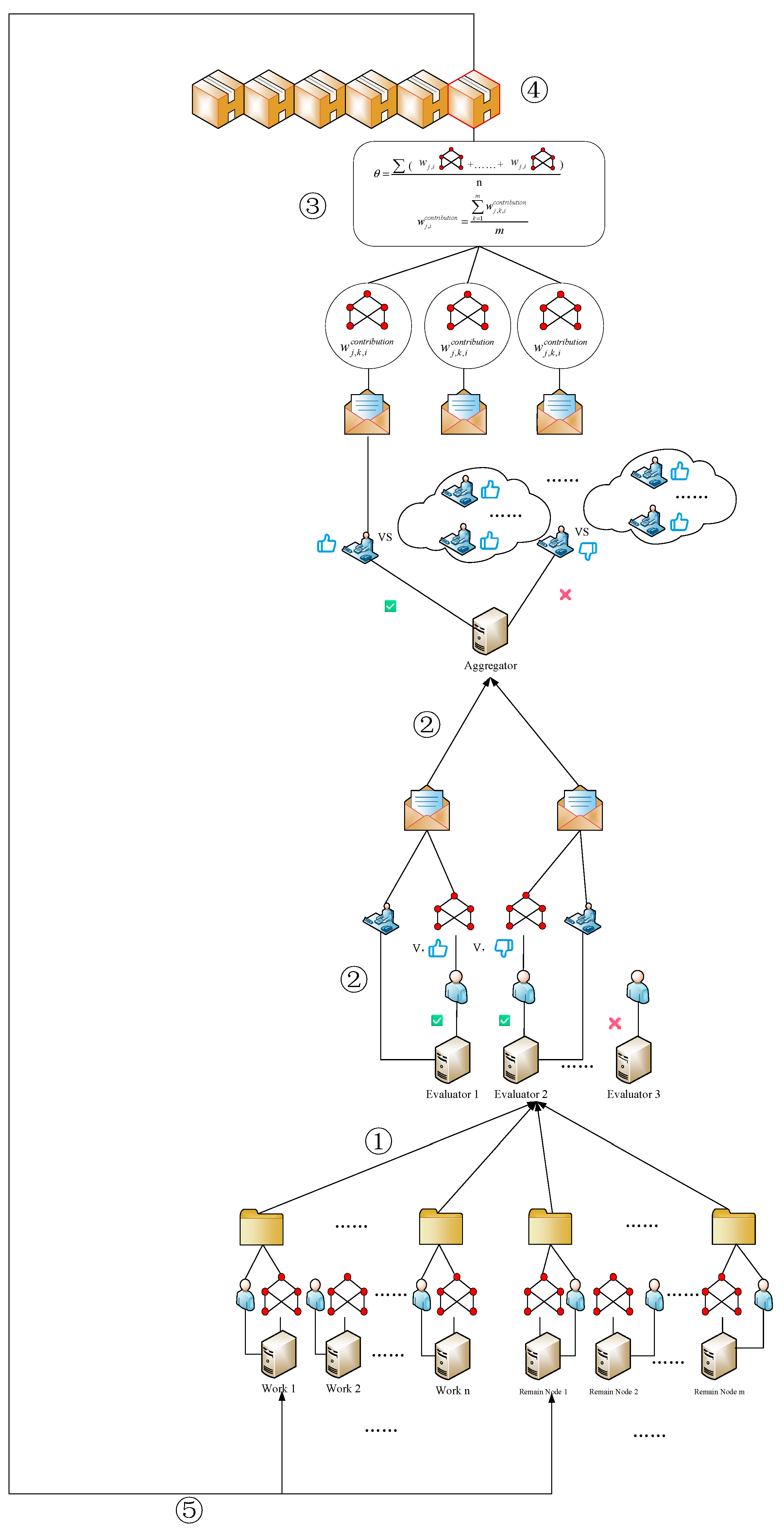
The implementation steps of the BDFL_NI_NTP scheme are shown in Figure 1.

Figure 1.
Blockchain and decentralized federated learning.
① In the th training round of federated learning, Worker node and Residual node train the local model using their private historical network traffic data, and the parameters of the model generated by the training are denoted as . Then, a transaction containing the hash value of model parameters and the identity certificate is generated, and the transaction is sent to all Evaluator nodes for evaluation.
② Evaluator node receives the transaction, verifies the identities of or , and extracts the model parameters for the nodes for evaluation. Evaluator node calculates the migration cost according to Equation (25) for the model parameters uploaded by nodes or , using local historical network traffic data. Compared with the best model with minimum migration cost, if the migration cost of the model does not exceed the threshold, the node is judged to be qualified, and it is rewarded and updated with the contribution value of the model; if not qualified, it is penalized and updated with the contribution value of the model. Then, pack the validation result and the hash value of model parameter , the contribution value of model, and the ID certificate of the Evaluator node to form a transaction , and send the transaction to the Aggregator node .
③ Aggregator node receives the transactions from all Evaluator nodes, and if an Evaluator and the majority of Evaluators have the same evaluation results, the result of its evaluation of the contribution value is taken into account; otherwise, the judgment of the Evaluator is ignored. If the majority of Evaluators assess the model that has parameters as passed, the model that has parameters will be included in the aggregation process. Meanwhile, for all the Worker nodes and Residual nodes, according to the contribution value judged by Evaluators, the average value is taken as the final value of contribution for each Worker and Residual node.
④ The Aggregator node performs model aggregation using Worker nodes, which are evaluated as passed in the aggregation process to generate the global model with parameters as well as the block .
⑤ Propagate the global model to all Worker and Residual nodes to ensure the next round of federated learning.
In the whole process described above, the evaluation result of Evaluator is supervised by Aggregator, and the aggregation process of Aggregator is supervised by the consensus mechanism.
- (2)
- Aggregation Method
The aggregation of Aggregator is to update the global model as follows:
where is the number of Worker nodes participating in the aggregation; is the weight factor of the local model , and the model with a larger predicted traffic value will be given a larger weight. Thus, the weight factor is calculated as:
where denotes the predicted traffic value of Worker node .
- (3)
- Role switching mechanism
In large-scale distributed networks, unfair switching of nodes may cause the model to deviate from normal updating during federated learning. In addition, frequent node switching can lead to resource waste and performance degradation [22]. It is important to be able to ensure the stability and efficiency of the system, but also to be able to quickly identify and punish nodes with malicious behaviors and reward nodes that work normally. Therefore, it is especially important to develop a reasonable role switching mechanism for nodes.
Initialization: First of all, in the initial state, there is no way to examine the working ability and working attitude of each node. Therefore, roles can be randomly assigned to nodes. After the initial role assignment is completed, the federated learning will be repeated.
Evaluation of Worker and Residual nodes: Then, the Worker node and the Residual nodes complete the training task locally and upload the trained model to the Evaluator node. The Evaluator node evaluates the model parameters uploaded by the nodes using the local historical network traffic data, and uses Equation (25) to calculate the migration cost using the predicted value of the model. The gap ratio is obtained by comparing the Worker node or the Residual node with the minimum value of migration cost as shown in the following equation:
where is the minimum value of migration cost calculated by Evaluator node for the current Worker node and the set of Residual nodes.
When the gap ratio is greater than the threshold , the current node is considered to have some malicious behavior. So, it is marked as a malicious behavior node, and its contribution value is reduced as shown in the following equation:
where is a constant value.
When the disparity ratio is less than the threshold value , the current node is considered to have no malicious behavior. Therefore, it is marked as a normal behavior node, and its contribution value is increased as shown in the following equation:
where is constant value.
Evaluation of Evaluator nodes: Evaluator will give the evaluation results of Worker nodes and Residual nodes to Aggregator, which is used to evaluate Evaluator for malicious behavior. If the number of Evaluator nodes with malicious behavior is high, the role switching process will be triggered. In addition, in order to avoid the system instability caused by frequent role switching, we set the role replacement to also be performed once every mini-round. During role switching, both normal working Aggregator nodes and Evaluator nodes no longer take up their original roles; they are reassigned contribution values and roles instead. If an Aggregator or Evaluator node has malicious behavior, its contribution value will be set to a smaller value, and its role will be switched to a Residual node. If the judgment of a Worker node is more reasonable, it is considered that it does not have malicious behavior. The degree of reasonableness of Evaluator judgment can be obtained based on the comparison of the judgment results with other Evaluators. The evaluation is calculated as follows for Evaluator :
where is the result of Evaluator ’s vote for Worker node or Residual node . When the vote is qualified, the value is 1, otherwise, the value is 0. is the similarity function; when the values of and are the same, the function value is 1, otherwise, the function value is 0.
When the value of is greater than the threshold , the evaluation result of the Evaluator is considered valid, and at the same time, it is considered that the Evaluator has no malicious behavior; otherwise, it is considered that its evaluation result is invalid, the Evaluator has malicious behavior, and it is necessary to mark it as a Residual node. When it starts to train the model in the next round, it cannot participate in the model aggregation. When the number of Evaluator nodes demoted as Residual nodes exceeds half of the maximum number of Evaluators, this round of federated learning is terminated, and the role switching process is started.
The evaluation results (e.g., model parameter scores, pass marks) of all Evaluators on Workers and Residual nodes are publicly recorded via the blockchain, and the recorded data are transparent and tamper-proof. Meanwhile, their evaluation results are also sent to Aggregator, which performs cross-validation based on the transactions uploaded by each Evaluator, and adopts Equation (31) to calculate the similarity, thereby enabling the Aggregator to supervise and manage the Evaluators based on their evaluation results.
Actual contribution values of Worker and Residual nodes: Finally, Aggregator calculates the actual contribution value of all Worker nodes and Residual nodes, i.e., the contribution value evaluated by all Evaluator nodes with normal behavior is averaged as shown in the following equation:
where, is the current number of Evaluator nodes.
3.3. Consensus Mechanism
Aggregator nodes may also have the possibility of intentionally tampering with the aggregation process, such as intentionally excluding certain valid models or inserting malicious models. At this point, a consensus mechanism is needed to verify and supervise the aggregation process of Aggregator. For example, the malicious behavior of an Aggregator node is determined by verifying if the list of qualified nodes selected by the Aggregator matches the results from non-malicious Evaluator nodes. Specifically, the model evaluation results (e.g., the list of qualified nodes) of all non-malicious Evaluator nodes on Worker nodes are publicly stored in the blockchain to ensure that the data cannot be tampered with. The Aggregator node is required to synchronize submission of the list of qualified Worker nodes selected for this round of aggregation when generating a block. The consensus mechanism compares the list of qualified nodes submitted by both parties, and if it is consistent, the Aggregator is considered to have no malicious behavior; if it is inconsistent, the Aggregator is considered to have malicious behavior, and the process of role switching is triggered.
In summary, the consensus mechanism must include the following points: (1) Worker nodes upload local model parameters with their own identifiers to ensure the credibility of the data. (2) The Evaluator node independently verifies the model and decides whether to accept the model through majority voting (e.g., more than half support). The voting result is recorded to the blockchain through a smart contract to ensure that it cannot be tampered with. (3) The Aggregator node collects the verified parameters and asynchronously aggregates them to generate the global model.
Therefore, the Consensus Mechanism includes the following four steps: (1) After all Worker and Residual nodes complete the upload of model parameters, if the uploaded model parameters meet the criteria, the smart contract rewards them with contribution value; otherwise, they are penalized in contribution value (Equations (28)–(30)). (2) At the start of the next round, the smart contract selects the Worker or Residual node with the highest contribution value (Equation (32)) as the Aggregator. Subsequently, nodes with higher contribution values are chosen as Evaluators, while the roles of the remaining nodes remain unchanged. This ensures that nodes with high contribution values (those without malicious behavior) can become committee members. (3) After the selected Evaluators generate evaluation results in the current round, the smart contract performs cross-verification by comparing the voting results of an Evaluator with those of others for similarity. If the similarity falls below a threshold, the Evaluator is deemed to exhibit malicious behavior. (4) After the selected Aggregator generates a new global model in the current round, the smart contract verifies the model by comparing the aggregation process with the evaluation results of non-malicious Evaluators stored on the blockchain. If the nodes participating in the aggregation are inconsistent with the evaluation results uploaded by non-malicious Evaluators, the Aggregator is judged to have engaged in malicious behavior.
Through the above mechanism, the system achieves efficient and secure consensus in the decentralized environment, while balancing the conflict between privacy protection and model performance.
3.4. Smart Contract
Smart Contract includes the following five steps: (1) Identity Verification: The smart contract verifies the identities of Worker, Residual, and Evaluator nodes. It writes the hash of the uploaded model parameters into blockchain transactions. (2) Transparent Recording and Execution: The smart contract records critical information (e.g., model parameter hashes, evaluation results, node contribution values, model aggregation rounds) on the blockchain to ensure integrity and traceability. Based on consensus mechanism verification results, the smart contract automatically adjusts node contribution values (deducting values for malicious nodes and increasing values for compliant nodes). (3) Committee Election: During role transitions, the smart contract automatically assigns new roles based on contribution value rankings. Worker or Residual nodes with higher contribution values have a greater probability of being selected as Aggregators. Subsequent nodes are more likely to become Evaluators, while the remaining nodes retain their roles as Workers or Residual nodes. (4) Malicious Node Monitoring: Committee members exhibiting malicious behavior are demoted to Residual nodes. If a significant number of Evaluators or Aggregators act maliciously, the role-switching mechanism is immediately triggered. (5) Non-Consecutive Committee Membership: Committee members without malicious behavior transition to Worker nodes in the next round. Malicious committee members become Residual nodes and are barred from participating in contribution value evaluations.
4. Algorithms
This section describes the proposed algorithms in detail. Algorithm 1 illustrates the entire algorithm process, while Algorithm 2 illustrates the node role switching algorithm process.
Since the consensus mechanism proposed in this paper involves dynamic and adaptive role switching, the algorithmic time complexity of the role switching mechanism is , where represents the number of nodes. For large-scale deployments involving thousands of nodes, the role switching process theoretically can be supported because its time complexity scales linearly only with the number of nodes.
| Algorithm 1: Blockchain and Decentralized Federated Learning Framework with Node Incentive |
| Inputs: Node set , Block and Global model . |
| Output: New block , New global model . |
| 1 For each node i: |
| 2 Randomize the type to which the nodes belong. |
| 3 End for |
| 4 For each node i: |
| 5 If node i belongs worker: |
| 6 ←0; |
| 7 End if |
| 8 End for |
| 9 For each round out_r from 1 to EPOCH_OUT: |
| 10 For each round in_r from 1 to EPOCH_IN: |
| 11 Train each local model using local private historical traffic data; //At Worker |
| 12 Generate transactions with the hash value of model parameter of each local model and authentication information, then send them to all Evaluator nodes; //At Worker |
| 13 For each model i: //At Evaluator |
| 14 If model i is worker or remain node: |
| 15 For each Evaluator : |
| 16 Verify the identity of the node; |
| 17 If identity passes: |
| 18 Evaluate the migration cost of the model i according to Equation (25); |
| 19 Compute the gap ratio according to Equation (28); |
| 20 If < threshold : |
| 21 Select the node and update the contribution according to Equation (30); |
| 22 Else: |
| 23 Ignore the node and update the contribution according to Equation (29); |
| 24 End if |
| 25 End if |
| 26 End for |
| 27 End if |
| 28 End for |
| 29 For each node k://At Aggregator |
| 30 If node k is evaluator: |
| 31 Compute evaluation for evaluator according to Equation (31); |
| 32 If evaluation > threshold : |
| 33 Generate a transaction containing the validation results and send it to the Aggregator node. |
| 34 Else: |
| 35 Set evaluator to be the remaining node; |
| 36 Set the contribution value of the remaining node k to 0; |
| 37 If the number of evaluator nodes is less than half the maximum number of evaluator nodes. |
| 38 TRANS = 1; |
| 39 Else: |
| 40 TRANS = 0; |
| 41 End if |
| 42 End if |
| 43 End if |
| 44 End for |
| 45 For each Worker://At Aggregator |
| 46 If more than half of the Evaluators select this worker. |
| 47 Select this worker as the aggregation node; |
| 48 End if |
| 49 End for |
| 50 For each worker://At Aggregator |
| 51 Calculate the actual contribution according to Equation (32); |
| 52 End for |
| 53 Generate global model and new block according to Equation (26) using all of the hash values of local models of the selected aggregator; |
| 54 Broadcast the new block to all Workers and the Remaining nodes. |
| 55 If TRANS==1: |
| 56 break; |
| 57 End if |
| 58 End for |
| 59 Reassign node roles according to Algorithm 2; |
| 60 End for |
| Algorithm 2: Node Role Assignment and Switching |
| Input: Current roles of all nodes. |
| Output: Updated node roles (Aggregator, Worker, Residual, or Evaluator nodes). |
| 1 Select a node as aggregator from the Workers and Residual nodes with the highest contribution; |
| 2 Select k nodes as evaluators from the Workers and Residual nodes with higher contribution; |
| 3 For each node i: |
| 4 If the node i is the former Evaluator or Aggregator: |
| 5 set the node i as Worker; |
| 6 End if |
| 7 End for |
| 8 Select n-m-1 nodes as Workers from the Workers and Residual nodes with higher contribution; |
| 9 Set the remaining nodes as Residual nodes; |
| 10 Return the result of the updated role assignment. |
5. Simulation
5.1. Settings
In this section, we use Python 3.6 and Pytorch 2.7 to verify the proposed scheme. The simulation platform is built on an Intel Core computer with a 1.8 GHz central processor and 8 GB Random Access Memory.
5.1.1. Parameter Settings
In the simulation, we obtain the network topology with scale: [200,991], where the numbers represent the quantity of NFV enabled nodes and physical links, respectively. The CPU capacity of nodes ranges from 100 to 200 cores, the storage capacity of nodes ranges from 100 to 200 GB, the processing capacity of nodes ranges from 80 to 150, the link bandwidth capacities between two nodes range from 15 to 25 Gbps, and the link latency between two adjacent nodes ranges from 1 to 2 s. The experiment considers eight types of VNFs. Each SFC randomly selects a few VNFs, and the length of each SFC is between 2 and 6. The SFC latency limit ranges from 30 to 50 s. There are 10 SFC requests in the network. The processing latency of VNF in service node is from 2 to 4 s. The CPU requirement of each VNF is from 1 to 2 cores, the storage requirement of each VNF is from 1 to 2 GB, the processing resource requirement of each VNF is from 1 to 2, and the bandwidth resource requirement of each virtual link is from 10 to 20 Mbps. In addition, the number of network service providers is 12.
Each local model contains 2-layer LSTM, with each hidden layer having 50 neurons. The input layer’s number of neurons corresponds to the state-space dimension, followed by two hidden layers, then the dueling network structure connected to the output layer. The output layer’s number of neurons corresponds to the discrete action space dimension. The algorithm uses SoftPlus as the activation function, with a maximum iteration number of 10.
Set up 12 federated learning participants, including 7 Workers (accounting for 58% of the total nodes) responsible for local model training and update uploads; 4 Evaluators (accounting for 33% of the total nodes) responsible for model parameter validation; and 1 Aggregator (accounting for 9% of the total nodes) responsible for global model aggregation.
Other parameter settings are shown in Table 2.
Table 2.
Parameter settings.
5.1.2. Data Sources
Network traffic data: Divide the network traffic data into time windows of 60 min each, and extract time-series features (e.g., traffic peaks). After standardization, split the data into a training set (60%), validation set (20%), and test set (20%).
NFV simulation data: Simulate a dynamic NFV environment to perform operations such as SFC mapping, VNF migration, and dynamic node joining and exiting.
5.1.3. Benchmark Schemes
We compare the performance of our proposed BDFL_NI_NTP approach against the following two baseline schemes. All three schemes are implemented using identical settings. More specifics regarding the two baseline schemes are as follows:
- (1)
- Baseline 1, FL: This is a network traffic prediction scheme based on a centralized server-based federated learning (FL) framework without a validation mechanism, where all local model parameters are directly aggregated [23].
- (2)
- Baseline 2, BlockFL: BlockFL is a decentralized architecture combining blockchain and federated learning, which adopts a committee-based validation mechanism for intermediate parameters. After training, nodes upload updates and trigger aggregation operations [20]. This model does not incorporate a role-switching mechanism.
We selected federated learning (FL) and BlockFL as baseline methods based on the following considerations:
- (1)
- Decoupling Objectives for Comparative Analysis: FL focuses on privacy preservation but lacks decentralization, while BlockFL introduces blockchain-based trust mechanisms yet remains vulnerable to malicious node attacks. Our method’s core innovation lies in simultaneously achieving decentralization and malicious attack resistance. By comparing with these single-objective solutions, we effectively demonstrate the necessity of multi-objective co-design (as evidenced by experimental results showing 59% and 155% reductions in loss values for FL and BlockFL, respectively, under malicious node attacks).
- (2)
- Scenario and Assumption Differences: Although the approach proposed in reference [14,15,16,17,18,19] (Section 2.2) shares some similarities with ours, the node roles in references [12,14,15,17] remain fixed. Only reference [19] supports adaptive node role changes—albeit based on computationally expensive () role-switching algorithms that scale poorly with edge device networks (training time increases exponentially). In contrast, our role-switching algorithm maintains time complexity, theoretically supporting significantly larger-scale deployments.
5.2. Evaluation Indicators
The following performance metrics are used to evaluate the performance of the algorithm:
- (1)
- Loss: It represents the average MSE loss of the predicted network traffic. It is defined as follows.where is MSE loss between the prediction value and actual value for the i-th data group, and is the total number of data points.
- (2)
- Latency: It represents the average migration latency of the physical network. It is defined as follows.where is analyzed in Equation (21).
- (3)
- Energy: The average amount of energy consumption of the network, which consists of energy consumption of all servers of the accepted SFC requests. It is defined as follows.where is defined in Equation (23).
- (4)
- Punish: It is the resource required by the failed SFC requests. An SFC request is said to be failed when it can not be embedded successfully. It can be defined as follows.where is defined in Equation (24).
- (5)
- Cost: It is the linear combination of the above three metrics, and it is defined as follows.where is calculated by Equation (25).
5.3. Performance Evaluation
To evaluate the effectiveness of BDFL_NI_NTP, we train the models using the parameters selected in the aforementioned analysis and deploy them in the federated learning (FL) module. The proportion of malicious nodes is uniformly set between 16% and 83%. Initially, we analyze the experimental results with six malicious nodes (50% of the total). We conducted five independent training runs and used the average of the prediction results as the final output for the presentation.
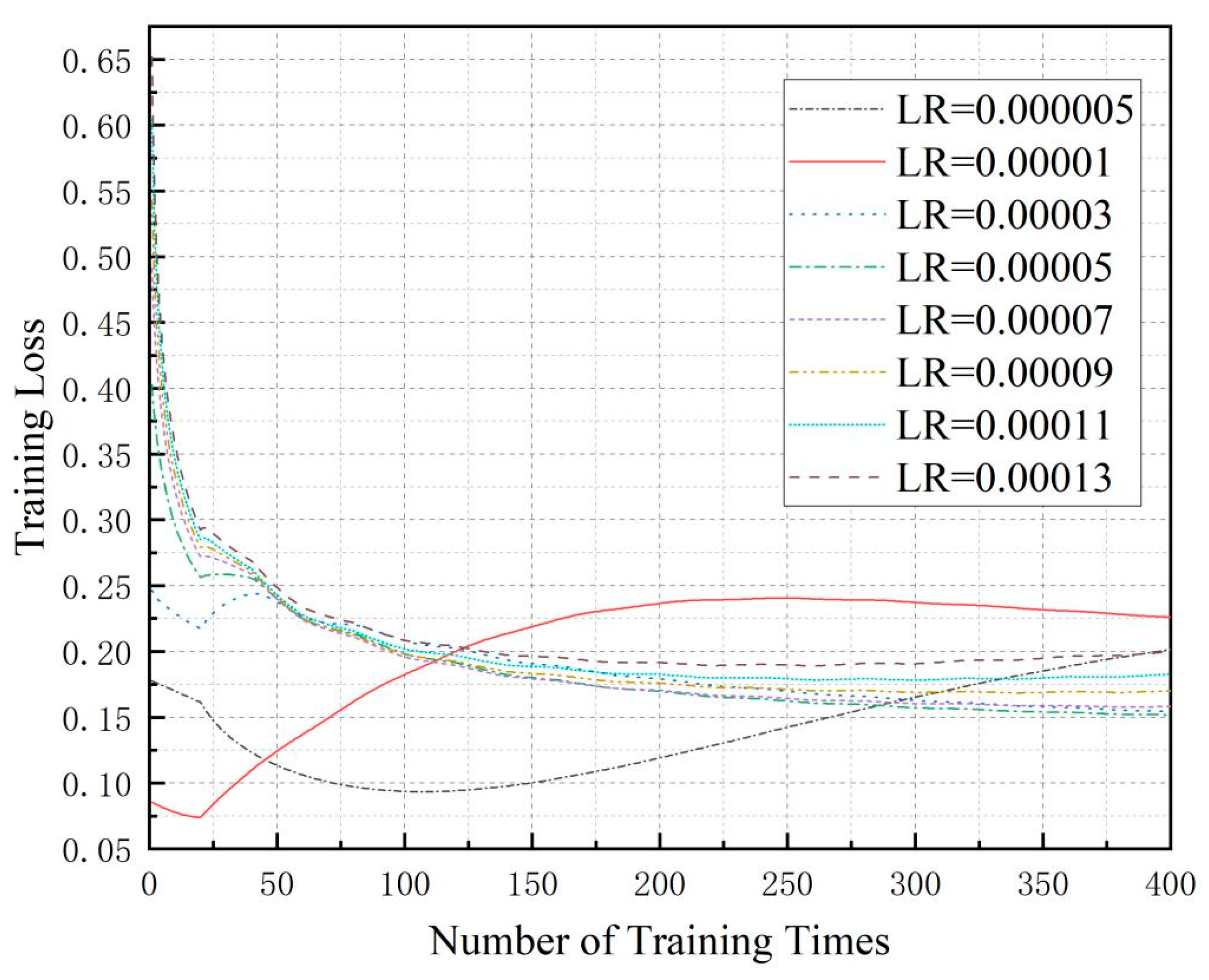
During the training process of our proposed BDFL_NI_NTP framework, we recorded the loss values. We conducted multiple training sessions with different learning rates (LR). The resulting curves showing the relationship between training epochs and loss values are presented in Figure 2.
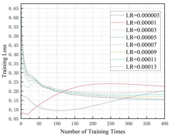
Figure 2.
Loss values of the validation data during the training process.
To comprehensively evaluate the training performance, we increased the number of iterations with the outer loop set to 20 cycles and the inner loop to 20 cycles. We recorded the reward values of the validation data during the training process. As can be seen in Figure 2, the experimental results of our BDFL_NI_NTP algorithm demonstrate distinct convergence behaviors under different learning rates (LRs): With smaller LRs (0.00001 and 0.000005), the model fails to converge within the same training epochs (20 × 20), while a larger LR (0.00013) achieves faster loss reduction but exhibits noticeable oscillations. Optimal convergence is observed within the moderate LR range (0.00003–0.00011). Mechanistically, an excessively high LR causes overshooting phenomena—where oversized parameter updates repeatedly bypass the loss function’s minima, resulting in unstable oscillations near the optimal solution. Conversely, an overly low LR substantially increases training costs due to sluggish loss reduction. Notably, appropriate oscillations may facilitate escaping local minima and discovering better global solutions.
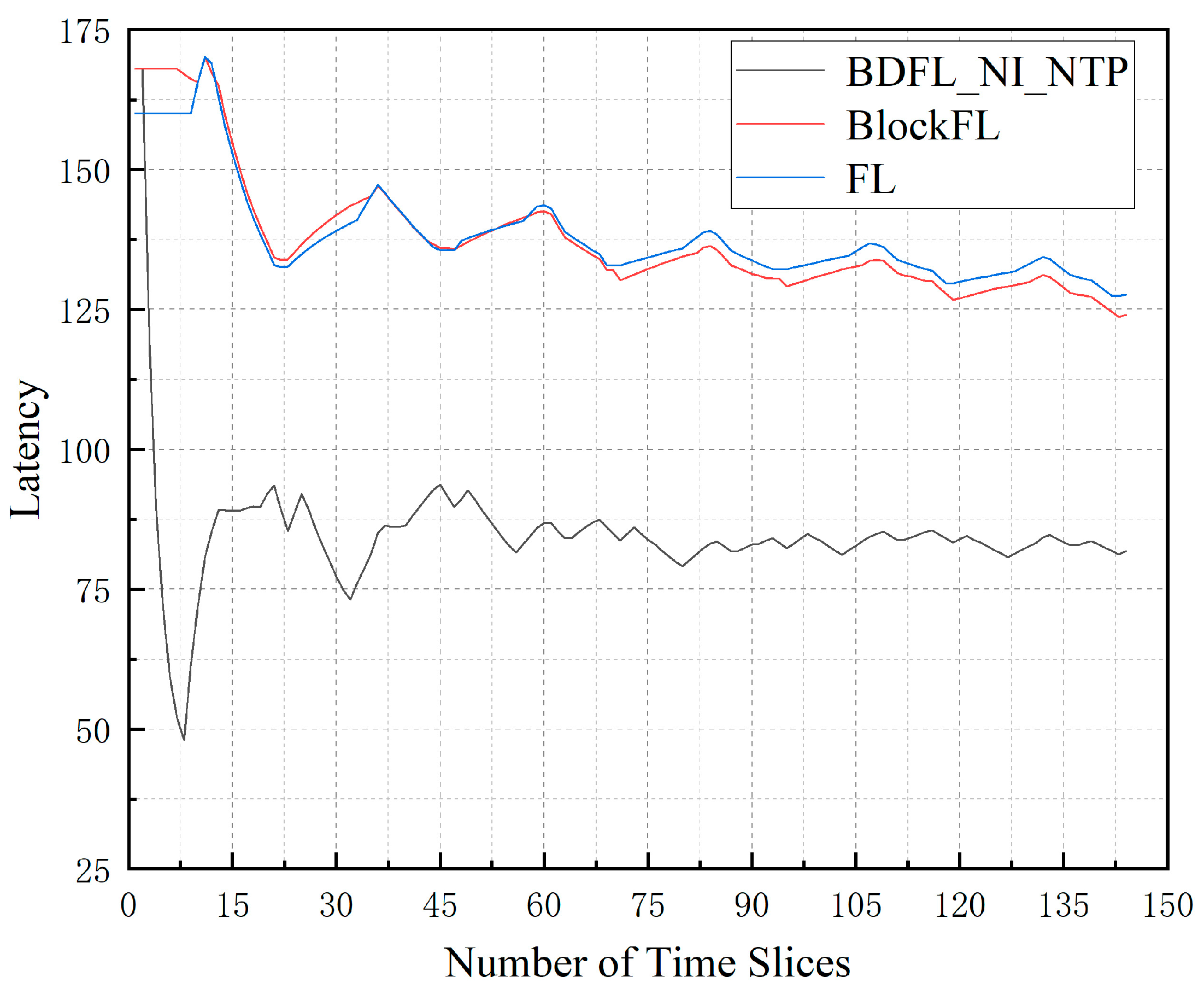
Next, we compare the migration latency, the energy consumption, the punishment of refused SFC requests, and the total cost of these algorithms during the prediction process.
Figure 3 illustrates the average migration latency of the three algorithms under the same environment. The latency value is an important metric in the migration process, which shows the migration cost in each time slice. It can be observed from the figure that the VNF migration latency value of the BDFL_NI_NTP algorithm is the lowest. Conversely, the VNF migration latency value of the FL algorithm is the highest. BlockFL increases by 51.60% compared to BDFL_NI_NTP; FL increases by 56.11% compared to BDFL_NI_NTP.
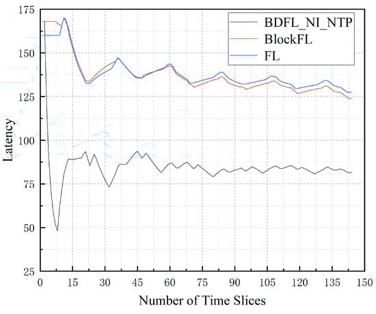
Figure 3.
Migration latency during the prediction process.
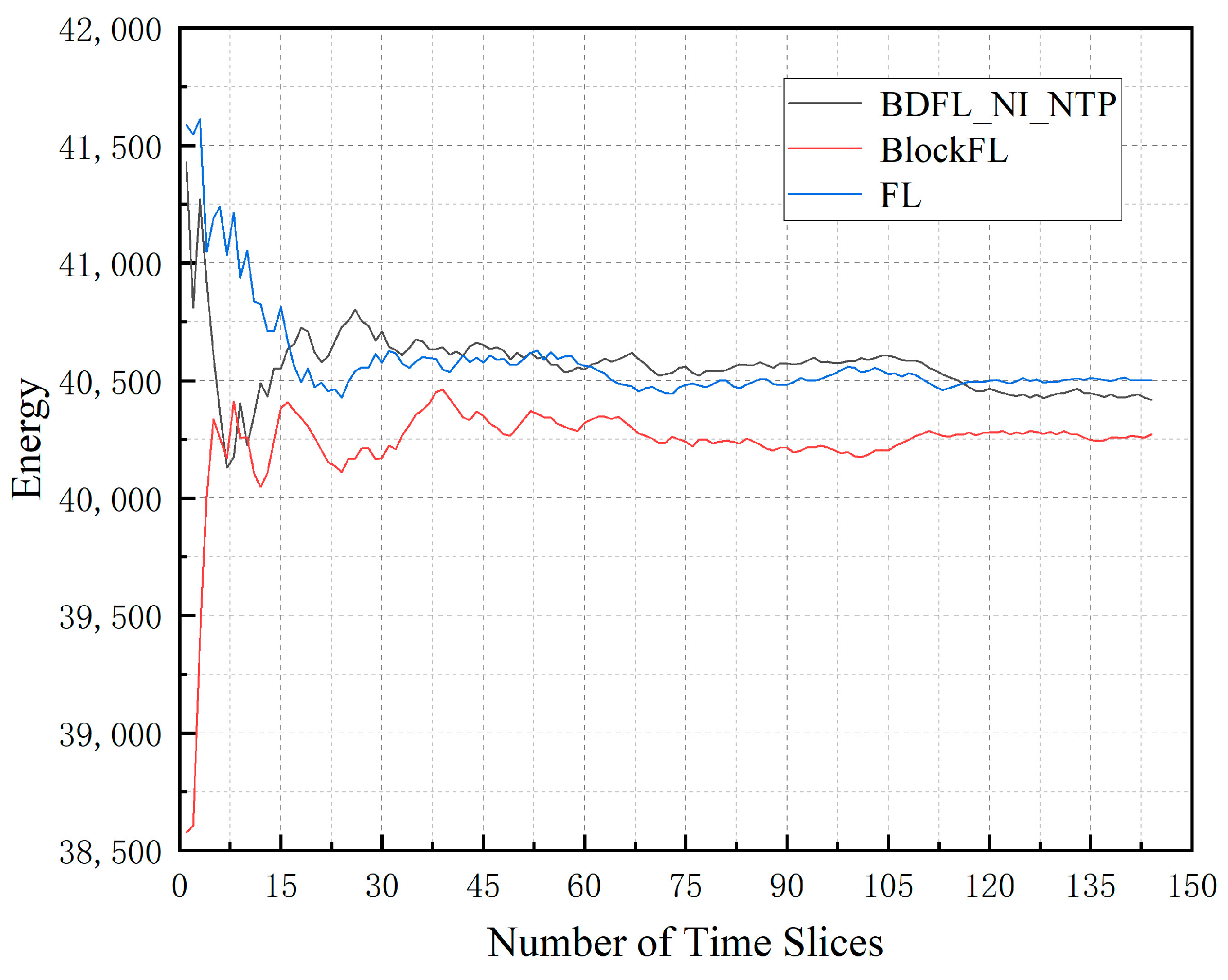
Figure 4 depicts the average energy consumption of the three algorithms under the same environment. BlockFL performs best in saving energy, but the differences among the three are not significant. FL increases by 0.21% compared to BDFL_NI_NTP; BlockFL decreases by 0.36% compared to BDFL_NI_NTP.
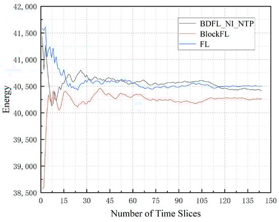
Figure 4.
Energy consumption during the prediction process.
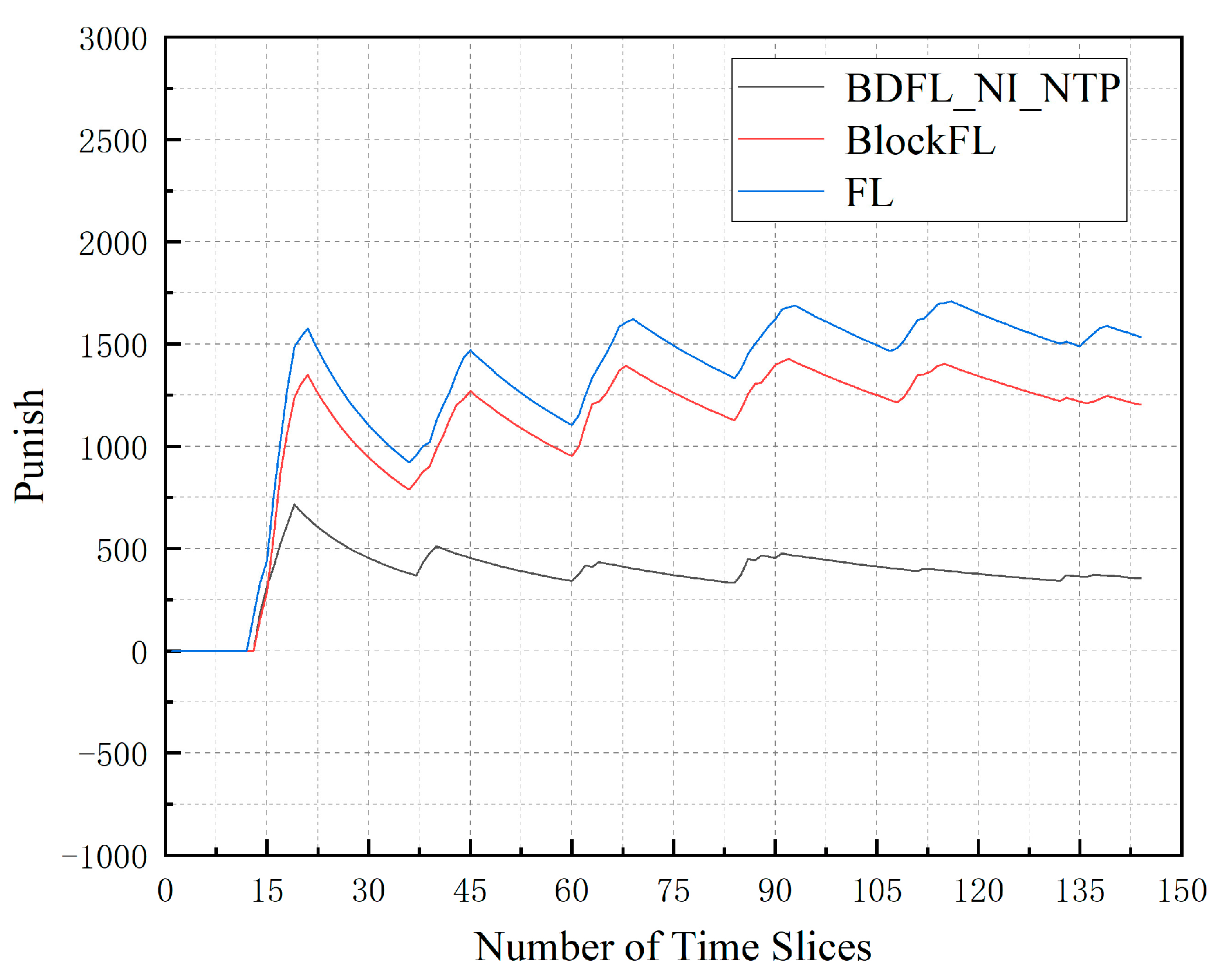
Figure 5 presents the total punishment for denying SFC requests of algorithms when the time slice number increases. We can observe that BDFL_NI_NTP achieves the lowest. BlockFL increases by 239.06% compared to BDFL_NI_NTP; FL increases by 332.36% compared to BDFL_NI_NTP.
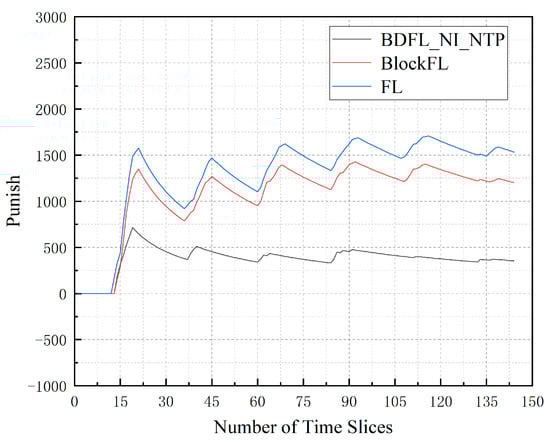
Figure 5.
The punishment for SFC requests denied during the prediction process.
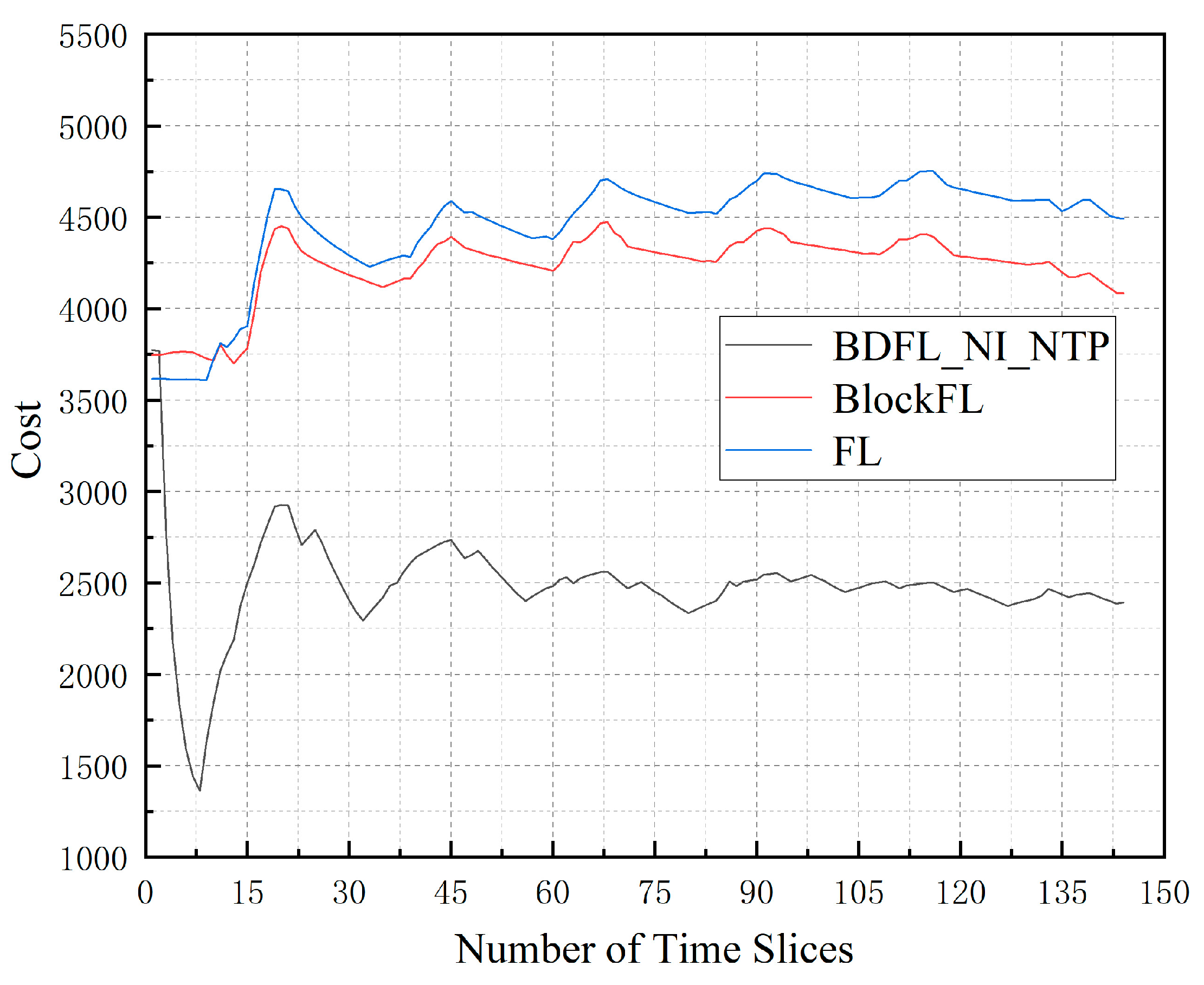
Figure 6 presents the average cost of the three algorithms when the time slice number increases. Through the above comparison, we find that BDFL_NI_NTP results in better performance. FL increases by 87.60% compared to BDFL_NI_NTP; BlockFL increases by 79.60% compared to BDFL_NI_NTP.
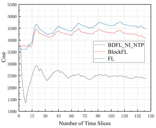
Figure 6.
The cost during the prediction process.
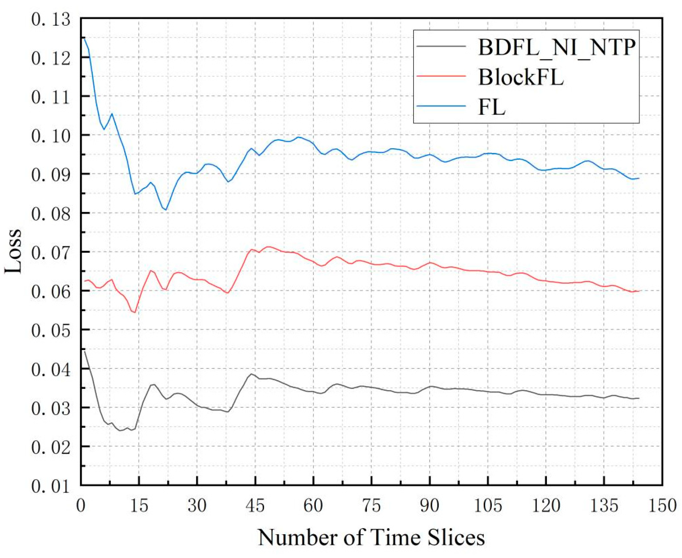
Figure 7 presents the average loss of the three algorithms when the time slice number increases. Through the above comparison, we find that BDFL_NI_NTP results in the best performance. FL increases by 85.73% compared to BDFL_NI_NTP; BlockFL increases by 174.67% compared to BDFL_NI_NTP.
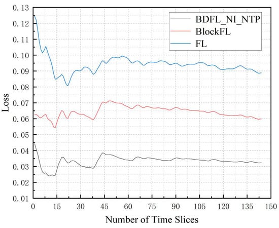
Figure 7.
The loss during the prediction process.
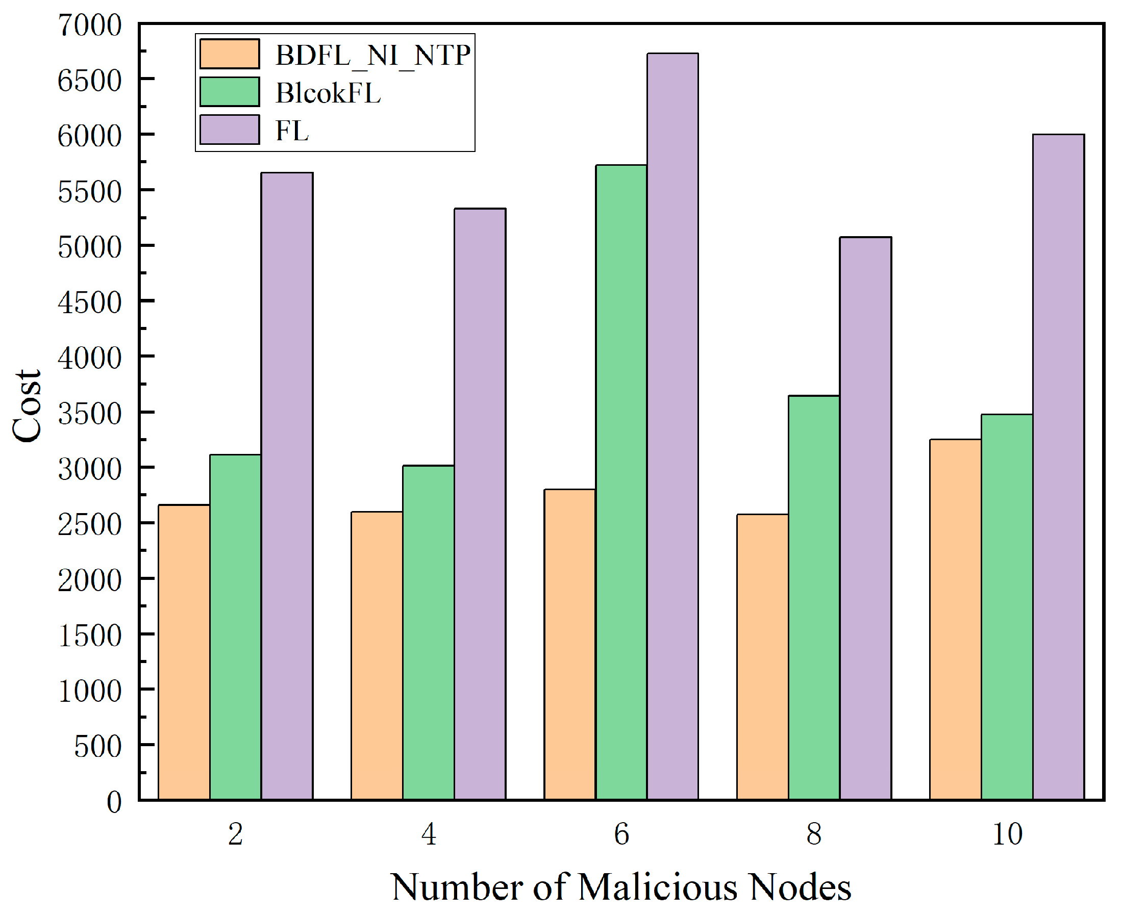
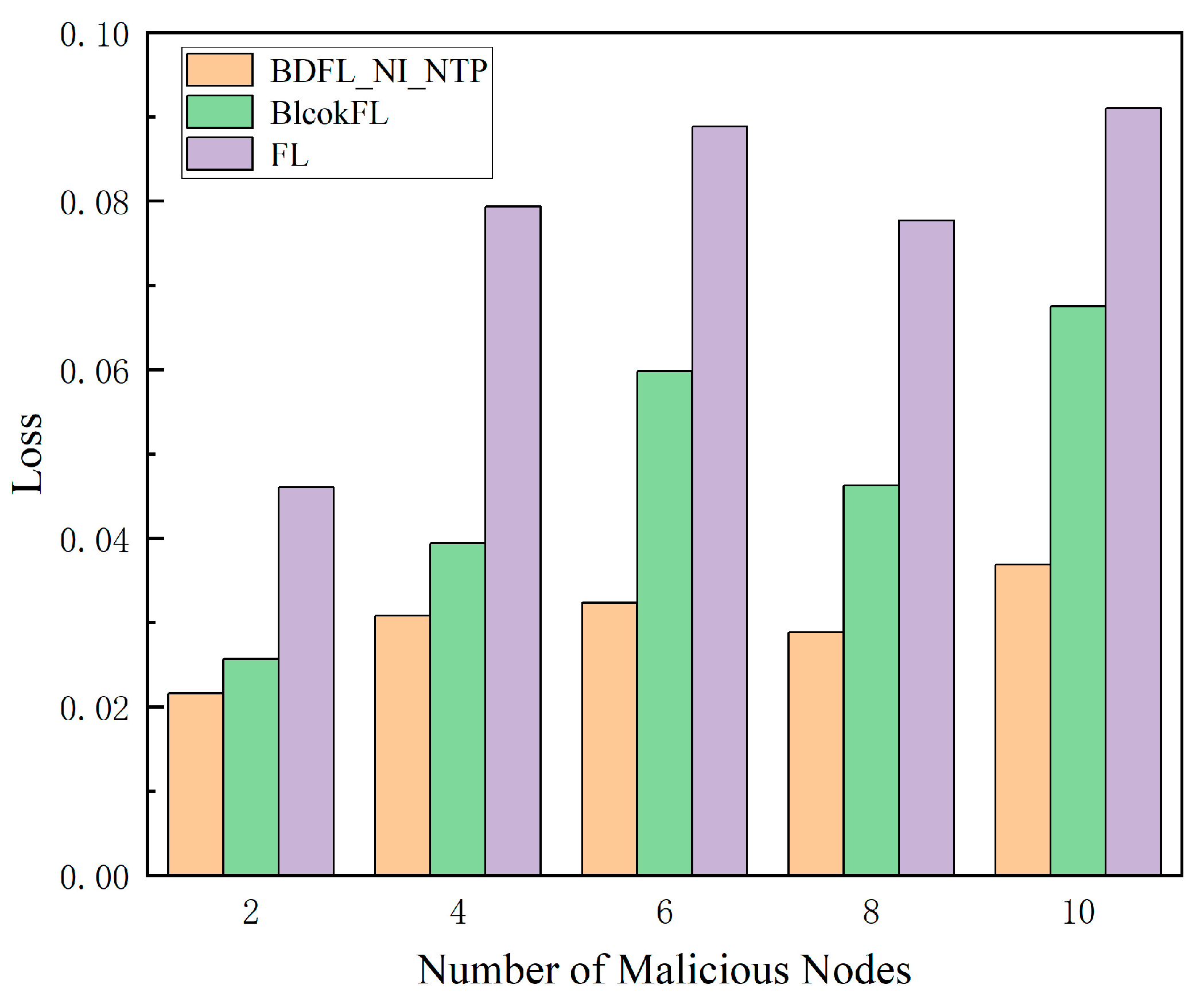
Finally, by varying the number of malicious nodes, the prediction results of the three algorithms are compared in terms of loss values, total costs, etc.
As shown in Figure 8 and Figure 9, as the proportion of malicious nodes increases, the migration cost and prediction loss value of the baseline algorithm’s prediction results increase, while our scheme BDFL_NI_NTP shows little change in terms of cost and prediction loss value.
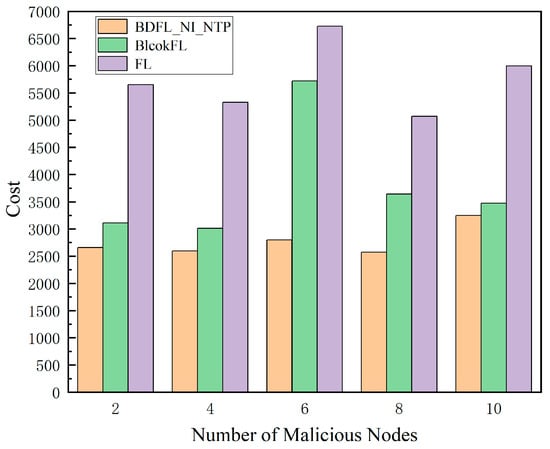
Figure 8.
Cost value under different malicious nodes.
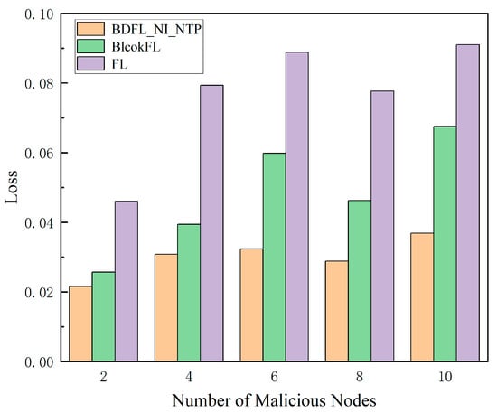
Figure 9.
Loss value under different malicious nodes.
Through comprehensive comparative analysis, our proposed method demonstrates remarkable advantages over both FL and BlockFL across multiple dimensions. In terms of prediction accuracy, it achieves a network traffic prediction loss of merely 3%, representing significant reductions of 58.69% and 154.57% compared to FL (4.77%) and BlockFL (7.66%), respectively. Regarding migration costs, as calculated by Equation (37), our solution reduces the cost to 2775.52 (a substantial 36.62% and 107.37% improvement over FL (3791.95) and BlockFL (5755.71)). Notably, while maintaining identical iteration counts, BDFL_NI_NTP introduces no significant computational overhead compared to BlockFL. These collective advancements not only resolve the traditional accuracy–efficiency trade-off dilemma but also provide a practical technical pathway for edge computing scenarios demanding high real-time performance and low resource consumption.
6. Conclusions
This study proposes a decentralized federated learning architecture for network function virtualization environments, with systematic experiments validating its three core advantages: (1) The privacy-preserving mechanism based on federated learning significantly reduces raw data leakage risks; (2) The blockchain consensus protocol with dynamic role switching achieves full decentralization, while the adaptive node role assignment method effectively mitigates malicious attacks; (3) The computationally efficient role-switching algorithm (complexity) ensures high training efficiency. The proposed solution is particularly suitable for real-time edge computing tasks and large-scale IoT collaborative inference scenarios.
Future work will focus on (1) developing lightweight model architectures via knowledge distillation or neural architecture search to reduce parameters; (2) designing cross-chain collaboration mechanisms with smart contracts for trustworthy multi-edge node incentives; and (3) extending scenario validation to vehicular networks and smart healthcare applications.
Author Contributions
Conceptualization, Y.H., B.L., J.L. and L.J.; methodology, Y.H., B.L., J.L. and L.J.; software, Y.H.; validation, B.L.; formal analysis, Y.H., B.L., J.L. and L.J.; resources, Y.H., B.L., J.L. and L.J.; writing—original draft preparation, B.L.; writing—review and editing, Y.H., B.L., J.L. and L.J.; visualization, B.L.; supervision, Y.H., B.L., J.L. and L.J.; project administration, Y.H., B.L., J.L. and L.J.; funding acquisition, Y.H. All authors have read and agreed to the published version of the manuscript.
Funding
This work was partially supported by the Henan Provincial Department of Science and Technology Program, grant number 242102210204.
Data Availability Statement
The data that support the findings of this study are available from the corresponding author upon reasonable request.
Acknowledgments
We extend our heartfelt appreciation to our esteemed colleagues at the university for their unwavering support and invaluable insights throughout the research process. We also express our sincere gratitude to the editor and the anonymous reviewers for their diligent review and constructive suggestions, which greatly contributed to the enhancement of this work.
Conflicts of Interest
The authors declare no conflicts of interest.
References
- Liu, Q.; Tang, L.; Wu, T.; Chen, Q. Deep reinforcement learning for resource demand prediction and virtual function network migration in digital twin network. IEEE Internet Things J. 2023, 10, 19102–19116. [Google Scholar] [CrossRef]
- Cai, J.; Zhou, Z.; Huang, Z.; Dai, W.; Yu, F.R. Privacy-preserving deployment mechanism for service function chains across multiple domains. IEEE Trans. Netw. Service Manag. 2024, 21, 1241–1256. [Google Scholar] [CrossRef]
- Kairouz, P.; McMahan, H.B.; Avent, B.; Bellet, A.; Bennis, M.; Bhagoji, A.N.; Bonawitz, K.; Charles, Z.; Cormode, G.; Cummings, R.; et al. Advances and open problems in federated learning. Found. Trends Mach. Learn. 2021, 14, 1–210. [Google Scholar] [CrossRef]
- Li, Z.; Yu, H.; Zhou, T.; Luo, L.; Fan, M.; Xu, Z.; Sun, G. Byzantine resistant secure blockchained federated learning at the edge. IEEE Netw. 2021, 35, 295–301. [Google Scholar] [CrossRef]
- Li, Q.; Li, X.; Zhou, L.; Yan, X. AdaFL: Adaptive client selection and dynamic contribution evaluation for efficient federated learning. In Proceedings of the ICASSP 2024—2024 IEEE International Conference on Acoustics, Speech and Signal Processing (ICASSP), Seoul, Republic of Korea, 14–19 April 2024; pp. 6645–6649. [Google Scholar] [CrossRef]
- Hou, Y.; Zhao, L.; Lu, H. Fuzzy neural network optimization and network traffic forecasting based on improved differential evolution. Future Gener. Comput. Syst. 2018, 81, 425–432. [Google Scholar] [CrossRef]
- Ramakrishnan, N.; Soni, T. Network traffic prediction using recurrent neural networks. In Proceedings of the 2018 17th IEEE International Conference on Machine Learning and Applications (ICMLA), Orlando, FL, USA, 17–20 December 2018; pp. 187–193. [Google Scholar] [CrossRef]
- Huang, C.-W.; Chiang, C.-T.; Li, Q. A study of deep learning networks on mobile traffic forecasting. In Proceedings of the 2017 IEEE 28th Annual International Symposium on Personal, Indoor, and Mobile Radio Communications (PIMRC), Montreal, QC, Canada, 8–13 October 2017; pp. 1–6. [Google Scholar] [CrossRef]
- Pan, C.; Zhu, J.; Kong, Z.; Shi, H.; Yang, W. DC-STGCN: Dual-channel based graph convolutional networks for network traffic forecasting. Electronics 2021, 10, 1014. [Google Scholar] [CrossRef]
- Huo, L.; Jiang, D.; Qi, S.; Miao, L. A blockchain-based security traffic measurement approach to software defined networking. Mobile Netw. Appl. 2021, 26, 586–596. [Google Scholar] [CrossRef]
- Qi, Y.; Hossain, M.S.; Nie, J.; Li, X. Privacy-preserving blockchain-based federated learning for traffic flow prediction. Future Gener. Comput. Syst. 2021, 117, 328–337. [Google Scholar] [CrossRef]
- Guo, H.; Meese, C.; Li, W.; Shen, C.C.; Nejad, M. B2SFL: A bi-level blockchained architecture for secure federated learning-based traffic prediction. IEEE Trans. Serv. Comput. 2023, 16, 4360–4374. [Google Scholar] [CrossRef]
- Kurri, V.; Raja, V.; Prakasam, P. Cellular traffic prediction on blockchain-based mobile networks using LSTM model in 4G LTE network. Peer-to-Peer Netw. Appl. 2021, 14, 1088–1105. [Google Scholar] [CrossRef]
- Feng, L.; Zhao, Y.; Guo, S.; Qiu, X.; Li, W.; Yu, P. BAFL: A blockchain-based asynchronous federated learning framework. IEEE Trans. Comput. 2022, 71, 1092–1103. [Google Scholar] [CrossRef]
- Li, J.; Shao, Y.; Wei, K.; Ding, M.; Ma, C.; Shi, L.; Han, Z.; Poor, H.V. Blockchain assisted decentralized federated learning (BLADE-FL): Performance analysis and resource allocation. IEEE Trans. Parallel Distrib. Syst. 2022, 33, 2401–2415. [Google Scholar] [CrossRef]
- Połap, D.; Srivastava, G.; Yu, K. Agent architecture of an intelligent medical system based on federated learning and blockchain technology. J. Inf. Secur. Appl. 2021, 58, 102748. [Google Scholar] [CrossRef]
- Cui, L.; Su, X.; Zhou, Y. A fast blockchain-based federated learning framework with compressed communications. IEEE J. Sel. Areas Commun. 2022, 40, 3358–3372. [Google Scholar] [CrossRef]
- Ren, Y.; Hu, M.; Yang, Z.; Feng, G.; Zhang, X. BPFL: Blockchain-based privacy-preserving federated learning against poisoning attack. Inf. Sci. 2024, 665, 120377. [Google Scholar] [CrossRef]
- Kasyap, H.; Manna, A.; Tripathy, S. An efficient blockchain assisted reputation aware decentralized federated learning framework. IEEE Trans. Netw. Service Manag. 2023, 20, 2771–2782. [Google Scholar] [CrossRef]
- Kim, H.; Park, J.; Bennis, M.; Kim, S.-L. Blockchained on-device federated learning. IEEE Commun. Lett. 2020, 24, 1279–1283. [Google Scholar] [CrossRef]
- Qiao, S.; Jiang, Y.; Han, N.; Hua, W.; Lin, Y.; Min, S.; Wu, X. LBFL: A lightweight blockchain-based federated learning framework with proof-of-contribution committee consensus. IEEE Trans. Big Data 2024. [Google Scholar] [CrossRef]
- Che, C.; Li, X.; Chen, C.; He, X.; Zheng, Z. A decentralized federated learning framework via committee mechanism with convergence guarantee. IEEE Trans. Parallel Distrib. Syst. 2022, 33, 4783–4800. [Google Scholar] [CrossRef]
- Yang, Q.; Liu, Y.; Chen, T.; Tong, Y. Federated machine learning: Concept and applications. ACM Trans. Intell. Syst. Technol. 2019, 10, 12. [Google Scholar] [CrossRef]
Disclaimer/Publisher’s Note: The statements, opinions and data contained in all publications are solely those of the individual author(s) and contributor(s) and not of MDPI and/or the editor(s). MDPI and/or the editor(s) disclaim responsibility for any injury to people or property resulting from any ideas, methods, instructions or products referred to in the content. |
© 2025 by the authors. Licensee MDPI, Basel, Switzerland. This article is an open access article distributed under the terms and conditions of the Creative Commons Attribution (CC BY) license (https://creativecommons.org/licenses/by/4.0/).