Tableau with Holes: Clarifying NP-Completeness

Abstract

In the context of defining $\mathcal{NP}$-completeness, a tableau represents a hypothetical accepting computation path p of a nondeterministic polynomial time Turing machine N on an input w. The tableau is encoded by the propositional logic formula $\psi$, defined as $\psi ={\psi }_{cell}\wedge {\psi }_{rest}$. The component ${\psi }_{cell}$ enforces the constraint that each cell in the tableau contains exactly one symbol, while ${\psi }_{rest}$ incorporates constraints governing the step-by-step behavior of N on w. Intuitively, ${\psi }_{rest}$ appears to pose a much greater challenge for satisfiability. This raises the question of whether the distinction between ${\psi }_{cell}$ being a 3cnf formula, rather than a cheap 2cnf formula, actually matters. We show that if, hypothetically, ${\psi }_{rest}$ can be succinctly represented as a Horn formula, then satisfying $\psi$ can be achieved efficiently in $K^{f(n,k)}$ steps, where N operates within $O\left(n^k\right)$ steps and both k and K are constants. Asymptotically, $f(n,k)\approx n^{{\displaystyle \frac{2}{3}}k}$. Our method has the potential for iterative application. Technically, we trim ${\psi }_{cell}$ down to a 2cnf–Horn formula, whose satisfiability allows for empty cells, or “holes”, in the tableau. This modified tableau represents exponentially many paths of N on w, rather than a single accepting path p. While a tableau with holes conceptualizes the satisfiability of ${\psi }_{trim}$—a trimmed-down version of $\psi$—it does not directly address the satisfiability of $\psi$. Therefore, we introduce an external user who efficiently employs backtracking to fill in specific holes, ultimately verifying the satisfiability of the original $\psi$.

1. Introduction

Consider an arbitrary nondeterministic polynomial time Turing machine N, running on arbitrary input w of length n, in $O\left(n^k\right)$ steps—where k is a constant. Formulating $\mathcal{NP}$-completeness entails representing the behavior of a hypothetical accepting computation path p of N on input word w, with

$$w=w_0{w}_1\dots w_{n-1},$$

using propositional logic. The path depends on the execution of uniquely labeled instructions, such as the following one:

$$t_{abc}:\left(q_1,a\right)\to \left\{\left(q_2,b,-\right),\left(q_3,c,+\right)\right\}.$$

This nondeterministic instruction, labeled $t_{abc}$, can be split into two distinct deterministic instructions as follows:

• $t_{ab}:\left(q_1,a\right)\to \left(q_2,b,-\right)$.
• $t_{ac}:\left(q_1,a\right)\to \left(q_3,c,+\right)$.

Each deterministic instruction is assigned a unique label (e.g., $t_{ab}$).

Instruction $t_{ab}$ specifies that when N is in state $q_1$ and reading symbol a, the machine is supposed to transition to state $q_2$ and rewrite the symbol a as b, and the tape head should move one cell to the left (−). A plus sign (+) indicates a unary move to the right.

Standard treatments of $\mathcal{NP}$-completeness use the concept of a tableau—a matrix with $n^k$ rows and $n^k+3$ columns, depicted in

Table 1. A tableau: an $n^k\times \left(n^k+3\right)$ matrix.

⊢	$q_0$	$w_0$	$w_1$	$w_2$	…	$w_{n-1}$	□	□	…	□	⊣
⊢											⊣
⊢											⊣
⊢											⊣

—to conceptualize the hypothetical computation path p. Each row in this tableau represents a Turing machine configuration of N, framed by boundary markers at the beginning and end. Successive rows evolve from their predecessors based on N’s transition function. A portion of one tableau, related to instruction $t_{ab}$, is shown on the left in

Table 2. The effect of instruction $t_{ab}$ is shown on the left, while the effect of instruction $t_{ac}$ is displayed on the right, with both figures read from top to bottom. Column indices range from $j-1$ to $j+1$.

a	$q_1$	a			a	$q_1$	a
$q_2$	a	b			a	c	$q_3$
$j-1$	j	$j+1$			$j-1$	j	$j+1$

, while a portion of another tableau, associated with instruction $t_{ac}$, is displayed on the right.

The two illustrations in Table 2 are slight variations of those presented by Sipser [1] (p. 280). In a similar vein, Papadimitriou introduces the concept of a “computation table” [2] (Section 8.2). Likewise, Hopcroft, Motwani, and Ullman use the term “array of cell/ID facts” [3] (p. 443). Finally, Aaronson also conveys the idea of a tableau, using slang in his popularizing book [4] (p. 61). To the best of our knowledge, all approaches to $\mathcal{NP}$-completeness rely on a tableau, ultimately tracing back to Cook’s seminal paper [5].

The symbol sequence “$q_{1}a$”, which appears in both top rows of Table 2, signifies that the machine is currently in state $q_1$, with its head oriented towards the tape cell containing the symbol a. This information is expressed propositionally through the conjunction of two Boolean variables, $x_{i,j,q_1}$ and $x_{i,j+1,a}$, where indices i and j denote the row i and column j in a tableau.

A tableau is deemed accepting when it represents a non-hypothetical accepting computation branch of N on w. The task of determining whether N accepts w is equivalent to ascertaining the existence of an accepting tableau for N on w. To achieve this, one must establish the satisfiability of $\psi$,

$$\psi ={\psi }_{cell}\wedge {\psi }_{rest},$$

a propositional logic formula that encodes the intended meaning of the tableau. This reasoning closely follows Sipser’s account [1] (Section 7.4).

To elucidate the variables within $\psi$, consider Q and $\Phi$ as, respectively, the state set and tape alphabet of N. Define $\mathcal{C}=Q\cup \Phi \cup \left\{⊢,⊣\right\}$, where ⊢ and ⊣ are boundary markers. For each i and j ranging from 1 to, respectively, $n^k$ and $n^k+3$, and for every symbol s in $\mathcal{C},$ we introduce a Boolean variable, $x_{i,j,s}$. We have a total of $O\left(n^{2k}\right)$ such variables.

Definition 1.

A Boolean formula in conjunctive normal form is referred to as a 3cnf formula if each clause consists of exactly three literals. If each clause contains at most two literals, the formula is called a 2cnf formula. We refer to a formula as “a 2cnf–Horn formula” if it qualifies as both a 2cnf and a Horn formula.

Remark 1.

More rigorous definitions can be found in Appendix A.

Remark 2.

Determining the satisfiability of 2cnf formulas or Horn formulas is substantially more efficient than for genuine 3cnf formulas [6].

1.1. Problem Statement

An accepting tableau provides a visual framework to demonstrate the satisfiability of $\psi$, affirming that N accepts w. The formula $\psi$ comprises two key components: ${\psi }_{cell}$ and ${\psi }_{rest}$, both expressed as 3cnf formulas. Intuitively, ${\psi }_{rest}$, which incorporates constraints pertaining to the step-by-step behavior of N on w, appears to pose a much greater challenge for satisfiability. This raises the question of whether the distinction between ${\psi }_{cell}$ being a 3cnf formula and being a cheap 2cnf formula actually matters.

1.2. Results

In this paper, we introduce our FHB algorithm (“Filling Holes with Backtracking”) along with its refinement, the rFHB algorithm. We show that if ${\psi }_{rest}$ can, hypothetically, be succinctly represented as a Horn formula, then the distinction between ${\psi }_{cell}$ being a 3cnf versus a simpler 2cnf formula becomes smaller. In this case, satisfying $\psi$ can be achieved with the rFHB algorithm in at most

$$K^{f(n,k)}$$

steps, where N operates within $O\left(n^k\right)$ steps and both k and K are constants. Here,

$$f(n,k)\approx {\left({\displaystyle \frac{n^{2k}}{4}}\right)}^{{\displaystyle \frac{1}{3}}}={\displaystyle \frac{n^{\frac{2k}{3}}}{1.59}},$$

or arguably even

$$f(n,k)\approx {\left({\displaystyle \frac{n^{2k}}{8}}\right)}^{{\displaystyle \frac{1}{4}}}={\displaystyle \frac{n^{\frac{k}{2}}}{1.68}}.$$

We further contextualize this result in Section 7. In future work, we will explain how the method presented in this article can be applied iteratively, progressively reducing the exponent $f(n,k)$.

1.3. Relevance

The immediate value of this work is twofold. First, it complements the author’s ongoing efforts to represent ${\psi }_{rest}$—specifically, the step-by-step behavior of certain well-chosen nondeterministic machines in particular contexts—using Horn clauses to the fullest extent possible. Second, it provides an analysis that tackles one of the first nontrivial questions—outlined below—that engineering students commonly ask when encountering $\mathcal{NP}$-completeness in standard treatments [1,6,7].

To illustrate part of this roadmap in a simplified manner, consider computational models with a constant number of nondeterministic choices. A conceptual example is solving a Sudoku puzzle, where constant nondeterminism can be leveraged as follows:

• Guess a number for a single Sudoku cell.
• After making this guess, follow the deterministic rules of Sudoku (each row, column, and box must contain the digits 1–9 exactly once) to fill in the rest of the grid.
• If the puzzle is unsolvable with that guess, try another guess for the same cell.

In this Sudoku context, the Turing machine’s step-by-step behavior is a priori known to be deterministic in large predefined regions of the tableau. As a result, it can naturally be expressed as a Horn formula in those regions. While this may be nearly trivial from a theoretical perspective, software engineers exploit such application-specific properties to optimize performance.

Remark 3.

In connection with related and upcoming results—where the author demonstrates how a binary choice an sich can be reformulated using a Horn formula—see his Turing machine simulation on YouTube (click here: https://youtu.be/3jmBcgjES5I (accessed on 4 April 2025)) and his theory building [8].

Mathematical engineers, in contrast, also seek to explore a broader, context-independent question: Given two 3cnf formulas, ${\psi }_{cell}$ and ${\psi }_{rest}$, which—if either—becomes easier to satisfy when the other is fully, yet hypothetically, transformed into an equivalent Horn formula? This theoretical question frequently arises among engineering students studying computational complexity, at least in the author’s experience.

In this paper, we assume that ${\psi }_{rest}$ can be reformulated as an equivalent Horn formula. The reverse hypothetical scenario—where we assume that ${\psi }_{cell}$ can be reformulated as a Horn formula—is not explored here.

1.4. Previous Work

Although contemporary accounts of $\mathcal{NP}$-completeness are widely available, there is a notable absence of studies specifically addressing holes in a tableau. Theoretically, each cell always contains a single symbol, both initially and throughout. See the previously cited works of Sipser, Papadimitriou, Hopcroft et al., and Aaronson. We aim to fill that void by enhancing and utilizing geometrical symmetry within the “tableau with holes” framework.

1.5. Methodology

This paper contributes to the field of $\mathcal{NP}$-completeness, with a focus on its foundational aspects. The research is supported by mathematical arguments, along with figures, tables, and graphs. While references to an off-the-shelf $\mathtt{HORNSAT}$ solver and algorithmic techniques (e.g., backtracking) stem not only from the literature but also from engineering practice, the content of this article is purely conceptual.

1.6. Outline

This paper is organized as follows. In Section 2, we refine the problem statement involving $\psi ={\psi }_{cell}\wedge {\psi }_{rest}$, and in Section 3, we introduce an auxiliary formula, ${\psi }_{extra}^{\eta }$. Then, we delve into the concept of a tableau with holes and prove three related claims in Section 4. Next, we present and analyze the proposed backtracking algorithm in Section 5, followed by a refinement thereof in Section 6. Finally, we present our conclusions in Section 7. This paper includes four appendices: standard definitions are given in Appendix A, lemmas are provided in Appendix B, a geometrical proof is presented in Appendix C, and a solution to a recurrence relation is derived in Appendix D.

2. Refining the Problem Statement

In a tableau, each of the $n^k\times \left(n^k+3\right)$ entries is referred to as a cell. Specifically, the cell located in row i and column j is denoted as $cell\left[i,j\right]$ and is supposed to contain a symbol from the set $\mathcal{C}$. The contents of these cells are represented using the variables of $\psi$. When the variable $x_{i,j,s}$ is assigned the value 1, it signifies that $cell\left[i,j\right]$ contains the symbol s. We also denote this situation as follows:

$$s@(i,j).$$

Similarly, we write

$$\neg s@(i,j)$$

or

$$\overline{s@(i,j)}$$

when $x_{i,j,s}$ is assigned 0. We use ¬ and the overbar interchangeably to enhance readability.

2.1. Formula ${\psi }_{cell}$

The 3cnf formula ${\psi }_{cell}$ is constructed as a conjunction of two segments, $S_1$ and $S_2$, structured as follows:

$$\begin{array}{ccc}{\psi }_{cell}& =& {\displaystyle \underset{1\le i\le n^k}{\bigwedge }\underset{1\le j\le n^k+3}{\bigwedge }\left(S_1\wedge S_2\right)}\\ S_1& =& {\displaystyle \underset{s\in \mathcal{C}}{\bigvee }{x}_{i,j,s}}\\ S_2& =& {\displaystyle \underset{s,t\in \mathcal{C},s\ne t}{\bigwedge }\left(\overline{x_{i,j,s}}\vee \overline{x_{i,j,t}}\right)}\end{array}$$

The first segment enforces that at least one variable is “turned on” per cell in the tableau, while the second segment ensures that at most one variable is “turned on” per cell. Although $S_2$ qualifies as a 2cnf–Horn formula, it is clear that $S_1$ is neither a 2cnf nor a Horn formula.

2.2. Formula ${\psi }_{rest}$

The second component of $\psi$ is defined as:

$${\psi }_{rest}={\psi }_{start}\wedge {\psi }_{accept}\wedge {\psi }_{step}.$$

The satisfiability of ${\psi }_{start}$, a 2cnf–Horn formula of size $O\left(n^k\right)$, guarantees that the initial row of the tableau represents the start configuration of N on w, of length n.

${\psi }_{start}$	=	$x_{1,1,⊢}\wedge x_{1,2,q_0}\wedge x_{1,3,w_0}\wedge x_{1,4,w_1}\wedge \dots \wedge x_{1,n+2,w_{n-1}}$
		$\wedge x_{1,n+3,\square }\wedge \dots \wedge x_{1,n^k+2,\square }\wedge x_{1,n^k+3,⊣}$

The boundary markers are denoted by ⊢ and ⊣, while □ represents the blank symbol.

The satisfiability of ${\psi }_{accept}$, a 2cnf–Horn formula of size $O\left(n^{2k}\right)$, entails that no cell in the tableau may contain the state symbol $q_{reject}$, thereby ensuring that an accepting tableau corresponds to a computation path p that does not reach the $q_{reject}$ state.

$${\psi }_{accept}=\underset{1\le i\le n^k}{\bigwedge }\underset{1\le j\le n^k+3}{\bigwedge }\overline{x_{i,j,q_{reject}}}$$

For readers unfamiliar with this convention, see Grädel [7] (p. 32).

To address the satisfiability of ${\psi }_{step}$, which captures the step-by-step behavior of N on w, we focus on the aforementioned instruction $t_{abc}$ as it applies to the following Turing machine configuration, denoted as C:

$$\dots a{q}_{1}a\dots$$

We analyze the execution of instructions $t_{ab}$ and $t_{ac}$ separately—both outcomes are depicted on the left and right sides of Table 2, respectively—before combining them into a single implication. This results in an expression of the form:

$$C_1\wedge C_2\wedge C_3\to T_{ab}\vee T_{ac},$$

where both $T_{ab}$ and $T_{ac}$ take the form $C_1\wedge C_2\wedge C_3$. Ultimately, this forms a 3cnf formula corresponding to Sipser’s notion of a $2\times 3$ window [1] (p. 280). By taking conjunctions over all $2\times 3$ windows defined by N, and for each row and column in the tableau, we derive a 3cnf formula ${\psi }_{step}$ of size $O\left(n^{2k}\right)$.

Whether the meaning of the formula ${\psi }_{step}$ can be compactly expressed as a Horn formula ${\psi }_{step}^{\eta }$ remains an open question. If one could answer this affirmatively, independent of a specific engineering context, it would provide a significantly simpler characterization of $\mathcal{NP}$-completeness than those found in the current textbooks. The only remaining non-Horn formula would be ${\psi }_{cell}$, whereas current accounts characterize $\mathcal{NP}$-completeness in terms of two non-Horn formulas: ${\psi }_{cell}$ and ${\psi }_{rest}$. See, for instance, Sipser [1] (Section 7.4).

Hypothetically, if such a Horn formula ${\psi }_{step}^{\eta }$ does exist, it must differ from ${\psi }_{step}$, i.e., ${\psi }_{step}\ne {\psi }_{step}^{\eta }$. The Greek letter eta ($\eta$), resembling the Latin letter h, is used here to highlight that the formula in question is a Horn formula.

By contrast, other formulas, such as ${\psi }_{start}$, are inherently Horn formulas:

$${\psi }_{start}={\psi }_{start}^{\eta }.$$

For simplicity and readability, however, we often write ${\psi }_{start}$ instead of ${\psi }_{start}^{\eta }$.

2.3. Trimming Down

Does the fact that ${\psi }_{cell}$ is a 3cnf formula inherently make $\psi$, with $\psi ={\psi }_{cell}\wedge {\psi }_{rest}$, computationally expensive to satisfy? To explore this question, we introduce one simplification, one assumption, and one extension—enabling a transition from $\psi$ to a trimmed-down formula, ${\psi }_{trim}$.

The simplification is as follows: we substitute the truth value of 1 for $S_1$ in ${\psi }_{cell}$, yielding ${\psi }_{cell}^{\prime }$, a 2cnf–Horn formula of size $O\left(n^{{\kappa }_1}\right)$, for some constant ${\kappa }_1$. The satisfiability of ${\psi }_{cell}^{\prime }$ allows for the presence of multiple empty cells, or “holes”, in the tableau.

The assumption is the existence of the Horn formula ${\psi }_{step}^{\eta }$, of size $O\left(n^{{\kappa }_2}\right)$, where ${\kappa }_2$ is a constant. Consequently, we now replace ${\psi }_{rest}$ with ${\psi }_{rest}^{\eta }$, defined as:

$${\psi }_{rest}^{\eta }={\psi }_{start}\wedge {\psi }_{accept}\wedge {\psi }_{step}^{\eta },$$

where Horn formula ${\psi }_{rest}^{\eta }$ is of size $O\left(n^{{\kappa }_3}\right)$, for some constant ${\kappa }_3$.

The extension involves introducing extra constraints, represented by ${\psi }_{extra}^{\eta }$, a Horn formula of size $O\left(n^{{\kappa }_4}\right)$, where ${\kappa }_4$ is a constant. We define ${\psi }_{extra}^{\eta }$ in the next section. The satisfiability of ${\psi }_{extra}^{\eta }$ is implied by the satisfiability of $\psi$.

From these three moves, we obtain:

$${\psi }_{trim}={\psi }_{cell}^{\prime }\wedge {\psi }_{rest}^{\eta }\wedge {\psi }_{extra}^{\eta },$$

where

$${\psi }_{trim}={\psi }_{trim}^{\eta }.$$

Horn formula ${\psi }_{trim}$ is of size $O\left(n^{{\kappa }_5}\right)$, for some constant ${\kappa }_5$.

Instead of working directly with $\psi$, we focus on ${\psi }_{trim}$ for the remainder of this paper. Typically, the tableau corresponding to a satisfiable ${\psi }_{trim}$ contains holes. Consequently, it does not encode a single accepting path p of N on w; instead, it indirectly represents exponentially many paths. From this point forward, unless explicitly stated otherwise, any discussion of tableaux and propositional variables will pertain to ${\psi }_{trim}$, not $\psi$.

Under significant nondeterminism (e.g., when the Turing machine N functions as a $\mathtt{SAT}$ solver processing a nontrivial input w), and given that $\psi$ is satisfiable, using an off-the-shelf $\mathtt{HORNSAT}$ solver $\mathcal{H}$ on the formula ${\psi }_{trim}$ leads to nearly all cells of the tableau containing holes.

This insight can be derived through conceptual reasoning or practical implementation via computer programming, both of which the author has employed. The worst-case assumption—that the $\mathtt{SAT}$ solver N makes several nondeterministic choices early in the computation—is realistic. Consequently, nearly all rows in the tableau remain undetermined, except for a few at the top.

Solver $\mathcal{H}$ assigns a default truth value of 0 (i.e., false) to each propositional variable, switching a value from 0 to 1 (i.e., true) only when compelled by the constraints of the given Horn clauses. The solver $\mathcal{H}$ never reverts a propositional variable assigned the value 1 back to 0. Since satisfying ${\psi }_{cell}^{\prime }$ is sufficient, rather than the full ${\psi }_{cell}$, solver $\mathcal{H}$ can satisfy ${\psi }_{trim}$ while leaving nearly all propositional variables turned off.

Remark 4.

To efficiently implement solver $\mathcal{H}$ with a few for loops, see the work of Dowling and Gallier [9].

Definition 2.

Given ${\psi }_{trim}$ and a corresponding tableau, we say that $cell[i,j]$ in the tableau contains a hole if $x_{i,j,s}$ is false for all $s\in \mathcal{C}.$

Definition 2 does not rule out the possibility that a specific variable $x_{i,j,s^{*}}$, for some $s^{*}\in \mathcal{C}$, may eventually be “turned on”, thereby filling the hole with symbol $s^{*}$ at a later stage. For instance, consider the case where $cell[i,j]$ contains a hole but is later filled by the user of solver $\mathcal{H}$ with the state symbol $q_5$, as illustrated in

Table 3. Crossing out 57 cells out of a total of $10\times 11=110$ cells.

	×	×	×	×	×
	×	×	×	×	×	×
	×	×	×	×	×	×	×				×
i	×	×	×	×	×	×	×	×	$q_5$	×	×
	×	×	×	×	×	×	×				×
	×	×	×	×	×	×
	×	×	×	×	×
	×	×	×	×
	×	×	×
	×	×
									j

. What are the implications of this action? To explore this, we now define the Horn formula ${\psi }_{extra}^{\eta }$.

3. Formula ${\psi }_{\mathit{e}\mathit{x}\mathit{t}\mathit{r}\mathit{a}}^{\eta }$

The formula ${\psi }_{extra}^{\eta }$ captures some global properties of a Turing machine computation. While it is redundant in the context of $\psi$’s satisfiability, it generally proves useful when ${\psi }_{trim}$ is satisfiable, i.e., when the tableau is potentially accepting but still contains holes. To formally define ${\psi }_{extra}^{\eta }$, we begin by examining the example in Table 3.

If $q_5@(i,j)$ holds, where $q_5\in Q$—meaning $x_{i,j,q_5}$ has a value of 1—then the tape head of N can never visit any of the crossed-out cells in Table 3. This restriction arises from the fact that a Turing machine can move its tape head only one cell to the left or right with each instruction and thus with each transition between consecutive rows in the tableau. Moreover, in each column of the tableau, all crossed-out cells either store or are expected to store the same tape symbol $s\in \Phi$. This restriction follows from the fact that a Turing machine can only modify a tape symbol when the head is positioned over that specific cell.

Therefore, filling the hole in $cell[i,j]$ with the state symbol $q_5$ effectively amounts to filling in all crossed-out cells, albeit indirectly. The requirement that $q_5@(i,j)$ holds implies that only cells that are not crossed out can contain the binary choices made by N on w.

Formula ${\psi }_{extra}^{\eta }$ expresses these restrictions as a conjunction of three parts:

$${\psi }_{extra}^{\eta }=\underset{1\le i\le n^k}{\bigwedge }\underset{1\le j\le n^k+3}{\bigwedge }\underset{q\in Q}{\bigwedge }\left[{\psi }_{extra}^{single}\wedge \underset{s\in \Phi }{\bigwedge }\left[{\psi }_{extra}^{left}\wedge {\psi }_{extra}^{right}\right]\right]$$

The single part, ${\psi }_{extra}^{single}$, ensures that at most one state symbol is stored per row. The left part, ${\psi }_{extra}^{left}$, addresses the crossed-out cells to the left of $q_5@(i,j)$ in Table 3, while the right part, ${\psi }_{extra}^{right}$, handles the crossed-out cells to the right.

Remark 5.

Technical simplifications are possible in the following discussion but would come at the cost of pedagogical clarity.

3.1. The Single Part

We define ${\psi }_{extra}^{single}$ as follows:

$${\psi }_{extra}^{single}=q@(i,j)\to \underset{q^{\prime }}{\bigwedge }\underset{j^{\prime }\ne j}{\bigwedge }\neg q^{\prime }@(i,j^{\prime }),$$

where $q^{\prime }\in Q$ and the column index $j^{\prime }$ ranges from 1 to $n^k+3$. This condition ensures that if the state symbol q is stored in $cell[i,j]$, it is the only state symbol in row i. In other words, no state symbol $q^{\prime }$ can be stored in any other cell within the same row.

Remark 6.

The possibility of $q^{\prime }@(i,j)$ with $q^{\prime }\ne q$ is ruled out due to the satisfiability of ${\psi }_{cell}^{\prime }$. Suppose that $q@(i,j)$ holds; then, according to ${\psi }_{cell}^{\prime }$, no other symbol (e.g., $q^{\prime }$) can be stored in $cell[i,j]$. Additionally, the reader will note that ${\psi }_{extra}^{single}$ can already be deduced from ${\psi }_{start}\wedge {\psi }_{step}^{\eta }\wedge {\psi }_{cell}^{\prime }$. Nonetheless, explicitly stating this property does no harm.

3.2. The Left Part

We define ${\psi }_{extra}^{left}$ as follows:

$${\psi }_{extra}^{left}={\psi }_1^{left}\wedge {\psi }_2^{left}\wedge {\psi }_3^{left}$$

On the one hand, we reason from row i both towards earlier rows ($-\delta$) and towards later rows ($+\delta$):

$${\psi }_1^{left}=\underset{0<m<j}{\bigwedge }\left[q@(i,j)\wedge s@(i,j-m)\to \underset{r\left(\delta \right)}{\bigwedge }s@(i\underset{+}{-}\delta ,j-m)\right],$$

where the restriction on $\delta$, denoted by $r\left(\delta \right)$, is defined by the following inequalities:

• $0\le \delta \le m-1.$
• $1\le i-\delta \le i+\delta \le n^k.$

Additionally, the expression

$$s@(i\underset{+}{-}\delta ,j)$$

is shorthand for:

$$s@(i-\delta ,j)\wedge s@(i+\delta ,j).$$

Example 1.

For instance, if $q_5@(i,j)$ and $s^{*}@(i,j-3)$ hold, then the following must also hold:

$$\underset{r\left(\delta \right)}{\bigwedge }[s^{*}@(i-\delta ,j-3)\wedge s^{*}@(i+\delta ,j-3)],$$

where $r\left(\delta \right)$ is defined by the following inequalities:

• $0\le \delta \le 2.$
• $1\le i-\delta \le i+\delta \le n^k.$

The reader can verify that all relevant cells range from $cell[i-2,j-3]$ at the top to $cell[i+2,j-3]$ at the bottom. These five cells correspond to the crossed-out entries in column $j-3$ in Table 3.

On the other hand, we reason from the earliest row ($i-{\delta }_{min}\left(m\right)$) and, respectively, the latest row ($i+{\delta }_{max}\left(m\right)$) toward row i:

$${\psi }_2^{left}=\underset{0<m<j}{\bigwedge }\left[q@(i,j)\wedge s@(i-{\delta }_{min}\left(m\right),j-m)\to s@(i,j-m)\right],$$

$${\psi }_3^{left}=\underset{0<m<j}{\bigwedge }\left[q@(i,j)\wedge s@(i+{\delta }_{max}\left(m\right),j-m)\to s@(i,j-m)\right],$$

where ${\delta }_{min}\left(m\right)$ is defined as the maximum (not the minimum) of the set:

$$\left\{\delta \right|0\le \delta \le m-1\mathrm{and}1\le i-\delta \le n^k\}.$$

Similarly, ${\delta }_{max}\left(m\right)$ is defined as the maximum of the set:

$$\left\{\delta \right|0\le \delta \le m-1\mathrm{and}1\le i+\delta \le n^k\}.$$

The satisfiability of ${\psi }_3^{left}$ ensures that if a specific cell, such as $cell[i+{\delta }_{max}\left(m\right),j-m]$ for some fixed m, is filled with the tape symbol $s^{*}$, then—through a chain reaction partially facilitated by ${\psi }_1^{left}$—all crosses in column $j-m$ are replaced with the symbol $s^{*}$. A similar observation applies to the satisfiability of ${\psi }_2^{left}$, which affects the propagation from an earlier cell, i.e., $cell[i-{\delta }_{min}\left(m\right),j-m]$.

3.3. The Right Part

Given the inherent symmetry of the problem, the formal definition of ${\psi }_{extra}^{right}$ closely mirrors that of ${\psi }_{extra}^{left}$ and is therefore omitted from this paper.

3.4. Consolidation

In summary, ${\psi }_{extra}^{\eta }$ is indeed a Horn formula, with a size of $O\left(n^{4k}\right)$, where the constant k corresponds to the running time $n^k$ of machine N. Furthermore, its satisfiability is trivially implied by the satisfiability of $\psi$. This last observation leads to the conclusion that if $\psi$ is satisfiable, then ${\psi }_{trim}$, with

$${\psi }_{trim}={\psi }_{cell}^{\prime }\wedge {\psi }_{rest}^{\eta }\wedge {\psi }_{extra}^{\eta },$$

is also satisfiable. Moreover, if ${\psi }_{trim}$ is satisfiable without any holes, then $\psi$ is also satisfiable, indicating that N accepts the input word w.

4. Tableau with Holes

We assume that ${\psi }_{trim}$ is satisfiable and that the tableau reflects this condition, typically containing several holes. A hole in the tableau, located at row index i and column index j, represents more than just an empty cell. To be conservative, we stipulate the following:

• Single Hole: If $cell[i,j]$ is the only hole in the tableau, it corresponds to at most $\mathsf{c}$ possible accepting computation paths, where $\mathsf{c}$ is the cardinality of $\mathcal{C}$. (In fact, in this scenario, it contributes to representing at most one accepting path.)
• Two Holes: If $cell[i,j]$ is one of two holes in the tableau, it contributes to representing up to $\mathsf{c}\times \mathsf{c}$ possible accepting computation paths.
• Three Holes: If $cell[i,j]$ is one of three holes, it contributes to representing up to $\mathsf{c}\times \mathsf{c}\times \mathsf{c}$ possible accepting computation paths.

This pattern continues, with each additional hole multiplying the maximum number of possible accepting computation paths by $\mathsf{c}$.

In the general case, the tableau, composed of a polynomial number of cells, indirectly represents an exponentially large number of paths for N on w, including paths that are syntactically inadmissible from the perspective of N’s step-by-step behavior. Among the syntactically admissible paths, there are both rejecting and accepting paths.

This flexibility is achieved by leaving most cells unfilled. The Horn clauses associated with ${\psi }_{trim}$ remain implicitly active in the background, waiting for an external user to fill in a hole via an additional specification, such as:

$$q^{*}@(i^{*},j^{*}).$$

Consequently, the solver $\mathcal{H}$ is called upon again, now tasked with satisfying

$${\psi }_{trim}\wedge q^{*}@(i^{*},j^{*}),$$

which stands for ${\psi }_{trim}\wedge x_{i^{*},j^{*},q^{*}}$. After two more user interventions, the solver is tasked with satisfying the following type of formula:

$${\psi }_{trim}\wedge q^{*}@(i^{*},j^{*})\wedge q^{**}@(i^{**},j^{**})\wedge q^{***}@(i^{***},j^{***}).$$

However, when the user’s guess, such as $q^{*}@(i^{*},j^{*}),$ leads the solver $\mathcal{H}$ to determine that the formula is unsatisfiable, backtracking becomes necessary. For instance, the user may replace $q^{*}@(i^{*},j^{*})$ with $q_{*}@(i^{*},j^{*})$, where $q^{*}\ne q_{*}$. Fortunately, as will be demonstrated by Claim 3 in this section, filling any hole in the center row of a convex polygon of holes scales the space for binary choices by a factor $\mathrm{\Delta }$, with $0\le \mathrm{\Delta }<1$.

The remainder of this section is divided into three parts. First, we give examples to build intuition (Section 4.1). Next, we increase the symmetry in our “tableau with holes” (Section 4.2). Third, we leverage this symmetry to establish three claims (Section 4.3).

4.1. Examples

The reader may compare Table 3 with

Table 4. Crossing out 59 cells out of a total of $10\times 11=110$ cells.

	×	×	×
	×	×	×	×
	×	×	×	×	×
i	×	×	×	×	×	×
	×	×	×	×	×	×	×				×
$i-2$	×	×	×	×	×	×	×	×	$q_5$	×	×
	×	×	×	×	×	×	×				×
	×	×	×	×	×	×
	×	×	×	×	×
	×	×	×	×
									j

, where the state symbol $q_5$ is positioned two rows lower (row $i-2$). In this example, filling a hole closer to the center horizontal line of the tableau proves slightly more effective, resulting in 59 crossed-out cells compared to 57 for the original position. However, this is not universally the case, as

Table 5. Crossing out 50 cells out of a total of $10\times 11=110$ cells.

	×										×
	×	×								×	×
i	×	×	×						×	×	×
	×	×	×	×				×	×	×	×
$i-2$	×	×	×	×	×	$q_5$	×	×	×	×	×
	×	×	×	×				×	×	×	×
	×	×	×						×	×	×
	×	×								×	×
	×										×
									j

illustrates.

To deepen intuition, three more observations can be made:

• Regardless of the specific placement of $q_5$ in row $i-2$ in Table 4, at least 50 out of the 110 cells will always be crossed out. This lower bound is illustrated in Table 5.
• Transitioning from Table 5 to a higher-resolution tableau of 15 by 16 cells, as depicted in

  Table 6. Crossing out 113 cells out of $15\times 16=240$ cells.

  1

  ×

  ×

  ×

  ×

  ×

  ×

  ×

  ×

  ×

  ×

  ×

  ×

  ×

  ×

  ×

  ×

  5

  ×

  ×

  ×

  ×

  ×

  ×

  ×

  ×

  ×

  ×

  ×

  ×

  ×

  ×

  ×

  ×

  ×

  ×

  ×

  ×

  ×

  ×

  ×

  ×

  ×

  ×

  ×

  ×

  ×

  ×

  ×

  ×

  ×

  8

  ×

  ×

  ×

  ×

  ×

  ×

  ×

  ×

  $q_5$

  ×

  ×

  ×

  ×

  ×

  ×

  ×

  ×

  ×

  ×

  ×

  ×

  ×

  ×

  ×

  ×

  ×

  ×

  ×

  ×

  10

  ×

  ×

  ×

  ×

  ×

  ×

  ×

  ×

  ×

  ×

  ×

  ×

  ×

  ×

  ×

  ×

  ×

  ×

  ×

  ×

  ×

  ×

  ×

  ×

  ×

  ×

  ×

  ×

  ×

  ×

  ×

  ×

  ×

  ×

  ×

  15

  ×

  1

  2

  3

  4

  5

  6

  7

  8

  9

  10

  11

  12

  13

  14

  15

  16

  , highlights a steady approach toward the limit of $50\%$ crossed-out cells.
• A second intervention in row 4 is shown in

  Table 7. Second intervention in row 4: crossing out 41 boldfaced cells out of 63 cells in rows 1–7.

  1

  ×

  ×

  ×

  ×

  ×

  ×

  ×

  ×

  ×

  ×

  ×

  ×

  ×

  ×

  ×

  ×

  ×

  ×

  ×

  ×

  ×

  ×

  ×

  ×

  ×

  ×

  ×

  ×

  ×

  ×

  ×

  ×

  ×

  ×

  ×

  ×

  ×

  ×

  ×

  ×

  ×

  ×

  ×

  ×

  $q_9$

  ×

  ×

  ×

  ×

  5

  ×

  ×

  ×

  ×

  ×

  ×

  ×

  ×

  ×

  ×

  ×

  ×

  ×

  ×

  ×

  ×

  ×

  ×

  ×

  ×

  ×

  ×

  ×

  ×

  ×

  ×

  ×

  ×

  ×

  ×

  ×

  ×

  ×

  ×

  ×

  ×

  ×

  ×

  ×

  ×

  ×

  ×

  8

  ×

  ×

  ×

  ×

  ×

  ×

  ×

  ×

  $q_5$

  ×

  ×

  ×

  ×

  ×

  ×

  ×

  ×

  ×

  ×

  ×

  ×

  ×

  ×

  ×

  ×

  ×

  ×

  ×

  ×

  10

  ×

  ×

  ×

  ×

  ×

  ×

  ×

  ×

  ×

  ×

  ×

  ×

  ×

  ×

  ×

  ×

  ×

  ×

  ×

  ×

  ×

  ×

  ×

  ×

  ×

  ×

  ×

  ×

  ×

  ×

  ×

  ×

  ×

  ×

  ×

  15

  ×

  1

  2

  3

  4

  5

  6

  7

  8

  9

  10

  11

  12

  13

  14

  15

  16

  , where the external user enforces $q_9@(4,12)$. This action results in 41 additional crossed-out cells.

Remark 7.

To simplify our exposition, the leftmost columns in our depicted tableaux do not contain the boundary marker ⊢. However, strictly speaking, column 1 should contain the boundary marker ⊢, while state and tape symbols appear only from column 2 onward.

A previously unmentioned detail regarding Table 5, Table 6 and Table 7 is that, due to the satisfiability of ${\psi }_{start}$, the state symbol $q_0$ must be positioned in the upper-left corner of the tableau. Consequently, all other cells in row 1 must be crossed out, and the additional crossed-out cells in

Table 8. A total of 120 crossed-out cells out of 240 cells due to ${\psi }_{start}$.

1

$q_0$

×

×

×

×

×

×

×

×

×

×

×

×

×

×

×

×

×

×

×

×

×

×

×

×

×

×

×

×

×

×

×

×

×

×

×

×

×

×

×

×

×

×

×

×

×

×

×

×

×

×

×

×

×

×

5

×

×

×

×

×

×

×

×

×

×

×

×

×

×

×

×

×

×

×

×

×

×

×

×

×

×

×

×

×

×

8

×

×

×

×

×

×

×

×

×

×

×

×

×

×

×

10

×

×

×

×

×

×

×

×

×

×

×

×

×

×

×

×

×

×

×

×

15

×

1

2

3

4

5

6

7

8

9

10

11

12

13

14

15

16

must also be accounted for.

We now discuss some specific base cases, where all rows but one contain a state symbol. Without loss of generality, the nondeterminism associated with Turing machine N consists solely of binary choices. For each such choice, say, between $t_1$ and $t_2$, the movement of $t_1$ is to the left (−), while the movement of $t_2$ is to the right (+).

The first base case is shown in

Table 9. Base case, resolved deterministically.

1

×

×

×

×

×

×

×

×

×

$q_6$

×

×

×

×

×

×

×

×

×

×

×

×

×

×

×

×

$q_7$

×

×

×

×

×

×

×

×

×

×

×

×

×

×

×

×

$q_8$

×

×

×

×

×

×

×

×

×

×

×

×

×

×

×

×

$q_9$

×

×

×

5

×

×

×

×

×

×

×

×

×

×

×

$q_{10}$

×

×

×

×

×

×

×

×

×

×

×

×

×

×

$q_{11}$

×

×

×

×

×

×

×

×

×

×

×

×

×

×

×

×

×

×

×

8

×

×

×

×

×

×

×

×

$q_5$

×

×

×

×

×

×

×

1

2

3

4

5

6

7

8

9

10

11

12

13

14

15

16

. Although the state $q_{11}@(6,11)$, with the value v stored in $cell[6,12]$, presents a binary choice between $t_1$ to the left and $t_2$ to the right, the presence of $q_5@(8,9)$ ensures that only $t_1$ can lead to an accepting tableau. Thus, this base case can be resolved automatically by the $\mathtt{HORNSAT}$ solver $\mathcal{H}$, without requiring any external user intervention. We realistically assume that ${\psi }_{step}^{\eta }$ addresses this deterministic scenario.

An initial true base case is depicted in

Table 10. Base case: a true binary choice, resolved by an external user.

1

×

×

×

×

×

×

×

×

×

$q_6$

×

×

×

×

×

×

×

×

×

×

×

×

×

×

×

×

$q_7$

×

×

×

×

×

×

×

×

×

×

×

×

×

×

×

×

$q_8$

×

×

×

×

×

×

×

×

×

×

×

×

×

×

×

×

$q_9$

×

×

×

5

×

×

×

×

×

×

×

×

×

×

×

$q_{10}$

×

×

×

×

×

×

×

×

×

×

×

×

×

×

$q_{11}$

×

×

×

×

×

×

×

×

×

×

×

×

×

×

×

×

×

×

8

×

×

×

×

×

×

×

×

×

×

$q_5$

×

×

×

×

×

1

2

3

4

5

6

7

8

9

10

11

12

13

14

15

16

. Since the path from row 1 to row 6 is fully determined, we can assume, without loss of generality, that a specific symbol, say, the symbol b, is stored in $cell[6,12]$. The binary choice in row 7 is then defined by, say, the following two instructions:

• $t_1:\left(q_{11},b\right)\to \left(q_2,b,-\right)$.
• $t_2:\left(q_{11},b\right)\to \left(q_3,c,+\right)$.

As a result, either $cell[7,10]$ or $cell[7,12]$ must contain the symbol $q_2$ or $q_3$, respectively. This problem features three holes and exhibits symmetry. Assuming the user selects $t_1$, he fills the hole in $cell[7,10]$ with the symbol $q_2$. Consequently, the other two holes are automatically filled in as well. Thus, in this base case, we achieve a filling factor of $100\%$.

What if we consider

Table 11. Base case: true binary choices, resolved by an external user.

100

×

×

×

×

×

×

×

×

×

$q_6$

×

×

×

×

×

×

×

×

×

×

×

×

×

×

×

×

$q_7$

×

×

×

×

×

×

×

×

×

×

×

×

×

×

×

×

$q_8$

×

×

×

×

×

×

×

×

×

×

×

×

×

×

×

×

$q_9$

×

×

×

105

×

×

×

×

×

×

×

×

×

×

×

$q_{10}$

×

×

×

×

×

×

×

×

×

×

×

×

×

×

$q_{11}$

×

×

×

×

×

×

×

×

×

×

×

×

×

×

×

×

×

×

108

×

×

×

×

×

×

×

×

×

×

$q_5$

×

×

×

×

×

1

2

3

4

5

6

7

8

9

10

11

12

13

14

15

16

instead? The only difference between this table and Table 10 lies in the indexing of the rows. Since the top row begins with index 100, there is no guarantee that the values of the crossed cells in this row are already determined. In this scenario, there could be multiple possible ways for N to transition from state $q_6$ to state $q_7$, each involving a movement of one unit to the right. As a result, the values of the crossed cells in the immediate vicinity of $q_{11}$ also remain undetermined. However, this situation is tangential to the main point. For, ultimately, there are at most ${\mathsf{c}}_{\mathsf{0}}$ ways to resolve the binary choices (plural) in row 107, where ${\mathsf{c}}_{\mathsf{0}}$ denotes the cardinality of Q. For example, in addition to $t_1$ and $t_2$ as specified earlier, suppose N also includes $t_3$ and $t_4$ as instructions originating from state $q_{11}$:

• $t_3:\left(q_{11},c\right)\to \left(q_8,a,-\right)$.
• $t_4:\left(q_{11},c\right)\to \left(q_{55},c,+\right)$.

Consequently, either $cell[107,10]$ will eventually hold $q_2$ or $q_8$, or $cell[107,12]$ will eventually hold $q_3$ or $q_{55}$. The external user selects one of ${\mathsf{c}}_{\mathsf{0}}$ possibilities, and the solver $\mathcal{H}$ automatically crosses out the remaining two holes accordingly, once again achieving a $100\%$ filling factor, regardless of whether $\mathcal{H}$ concludes with “satisfiable” or “unsatisfiable”.

4.2. Enhancing Symmetry

Let us now adopt a more rigorous approach. A tableau with holes can be viewed geometrically as a collection of one or more convex polygons, each representing a maximum pocket of holes within the tableau.

When a straight line cuts a convex polygon, it divides the polygon into two smaller convex polygons. We assume familiarity with the following definition and lemma:

Definition 3.

A polygon is a closed, two-dimensional geometric figure made up of a finite number of straight line segments. These segments, called edges or sides, are joined pairwise at their endpoints, known as vertices. The sides of a polygon do not cross each other, and the figure encloses a region in a plane. A convex polygon is a polygon in which all interior angles are less than ${180}^{\circ }$, and every line segment drawn between any two points inside the polygon lies entirely within the polygon.

Lemma 1 (Cutting a Convex Polygon with a Straight Line).

A straight line that intersects a convex polygon will divide the polygon into exactly two convex polygons, provided the line does not pass solely through one vertex or lie entirely along an edge.

Example 2.

Consider an initially empty $15\times 16$ tableau, constituting a convex polygon P. Suppose, for illustrative purposes, that it is the user who injects $q_0@(1,1)$ into the tableau. As shown in Table 8, this action results in a straight line of crosses spanning from $cell[1,2]$ to $cell[15,16]$ that intersects P. This line forms a ${45}^{\circ }$ angle with both the horizontal and vertical edges of P.

To further refine the symmetry of our geometric perspective, we introduce a few additional assumptions about the Turing machine N and its tableau representation. These assumptions are made without loss of generality.

First, we disregard boundary markers in our geometric considerations. As a result, column 1 directly contains state and tape symbols, while the rightmost column is indexed as $n^k+1$. Formally, boundary markers can be included in our discourse if needed, but they are omitted here for simplicity.

Second, we assume that machine N processes only inputs w of even length. This condition can be ensured by designing the encoding function from natural numbers to strings w to enforce this property [10]. The implication is that $n^k$ and ${\displaystyle \frac{n^k}{2}}$ are always even and $n^k+1$ and ${\displaystyle \frac{n^k}{2}}+1$ are always odd, thereby simplifying our forthcoming case analysis.

Third, we emphasize that, after performing at most $O\left(n^k\right)$ steps, an accepting Turing machine N does not halt upon reaching the $q_{accept}$ state (see Definitions A4 and A5). Moreover, we now generalize as follows: the machine need not remain in the $q_{accept}$ state, as long as it does not enter the $q_{reject}$ state (recall the definition of ${\psi }_{accept}$ in Section 2.2). Going forward, we assume that the satisfiability of ${\psi }_{accept}$ ensures that N roams in the $q_{accept}$ state around the central column ${\displaystyle \frac{n^k}{2}}+1$, moving towards the bottommost rows of the tableau. Specifically, the condition

$$q_{accept}@(n^k-ϵ,{\displaystyle \frac{n^k}{2}}+1),$$

must hold for some $ϵ\in \{0,1\}$. In fact, we aim to assert shortly that $ϵ=0$.

Remark 8.

Just like machine N with $ϵ\in \{0,1\}$, it is possible to design nondeterministic Turing machine $N^{″}$, which operates in $O\left(n^{k^{″}}\right)$ time for some constant $k^{″}$, such that $ϵ=0$. Suppose nondeterministic Turing machine $N^{\prime }$, running in $O\left(n^{k^{\prime }}\right)$ time for some constant $k^{\prime }$, with $k^{\prime }>k$, operates similarly to our original machine N, but with two tapes instead of one. The second (auxiliary) tape contains $n^{k^{\prime }}$ strokes before the computation of $N^{\prime }$ on w begins. We can make this assumption because any reasonable encoding function that maps natural numbers to string representations on the Turing machine’s tapes is of our choosing. As $N^{\prime }$ processes the input word w on its first tape, it simultaneously erases one stroke per step on the auxiliary tape. Once $N^{\prime }$ has finished processing w on the first tape and has entered the $q_{accept}$ state, it ignores the first tape altogether and uses the remaining strokes on the auxiliary tape to determine how to enter or re-enter the $q_{accept}$ state at $cell[n^{k^{\prime }},{\displaystyle \frac{n^{k^{\prime }}}{2}}+1]$. The two-tape machine $N^{\prime }$ is converted into the equivalent one-tape Turing machine, $N^{″}$, with a polynomial overhead. Thus, we now have a nondeterministic one-tape Turing machine $N^{″}$, operating in $O\left(n^{k^{″}}\right)$ time, ensuring that

$$q_{accept}@(n^{k^{″}},{\displaystyle \frac{n^{k^{″}}}{2}}+1)$$

holds if and only if N accepts w within $O\left(n^k\right)$ time.

Building on the insights provided from Remark 8, and with a harmless abuse of notation, we assume that for machine N the satisfiability of ${\psi }_{accept}$ guarantees $ϵ=0$. In other words, the condition

$$q_{accept}@(n^k,{\displaystyle \frac{n^k}{2}}+1)$$

is satisfied if and only if N on w accepts.

The caveat, however, is that encoding a natural number as an input string on the tape of N does not necessarily comply with the stipulations defined by ${\psi }_{start}$ earlier in this paper (see Section 2.2). Simulating a two-tape Turing machine with a one-tape Turing machine requires a setup different from the assumptions made thus far. Furthermore, to enhance geometric symmetry, we aim for the satisfiability of ${\psi }_{start}$ to ensure that the state symbol $q_0$ is placed at the center of the first row, rather than in the leftmost cell.

This implies the following: the symbol $q_0$ in row 1 is flanked by alternating stroke symbols and half of the input to its immediate left, while the other half of the input is interspersed with strokes on its immediate right. All other cells, with the exception of the boundary markers, contain the blank symbol □. The precise details of this arrangement are not central to our discussion. More important is that the input word w has an even length n (as noted earlier), which in turn ensures that both $n^k$ and ${\displaystyle \frac{n^k}{2}}$ are also even. Specifically, the satisfiability of ${\psi }_{start}$ guarantees that the following condition is met:

$$q_0@(1,{\displaystyle \frac{n^k}{2}}+1).$$

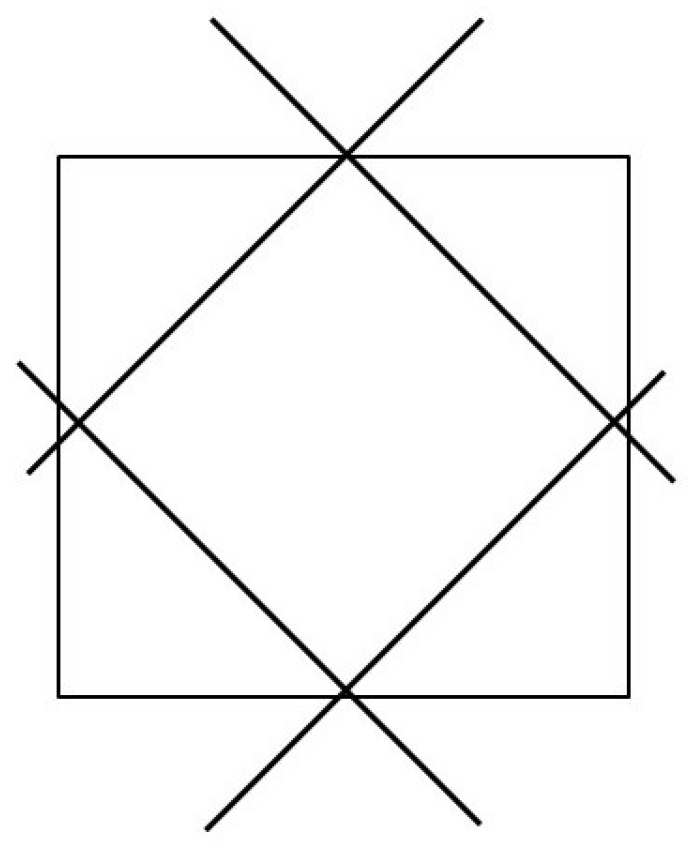
To enhance symmetry one final time, we add an extra row at the bottom, forming a square grid with $n^k+1$ rows and $n^k+1$ columns, as shown in Figure 1. The top cross corresponds to ${\psi }_{start}$, while the bottom cross represents ${\psi }_{accept}$. Consequently, for accepting w, machine N remains in the $q_{accept}$ state or re-enters it upon visiting $cell[n^k+1,{\displaystyle \frac{n^k}{2}}+1]$, instead of making this stipulation for $cell[n^k,{\displaystyle \frac{n^k}{2}}+1]$.

Table 12. Symmetry in full display, where “$q_{acc}$” is an abbreviation for “$q_{accept}$”.

1

×

×

×

×

×

×

×

×

$q_0$

×

×

×

×

×

×

×

2

×

×

×

×

×

×

×

×

×

×

×

×

×

×

3

×

×

×

×

×

×

×

×

×

×

×

×

4

×

×

×

×

×

×

×

×

×

×

5

×

×

×

×

×

×

×

×

6

×

×

×

×

×

×

7

×

×

×

×

8

×

×

9

10

×

×

11

×

×

×

×

12

×

×

×

×

×

×

13

×

×

×

×

×

×

×

×

14

×

×

×

×

×

×

×

×

×

×

15

×

×

×

×

×

×

×

×

×

×

×

×

16

×

×

×

×

×

×

×

×

×

×

×

×

×

×

17

×

×

×

×

×

×

×

×

$q_{acc}$

×

×

×

×

×

×

×

×

1

2

3

4

5

6

7

8

9

10

11

12

13

14

15

16

17

illustrates this, with $n^k=16$.

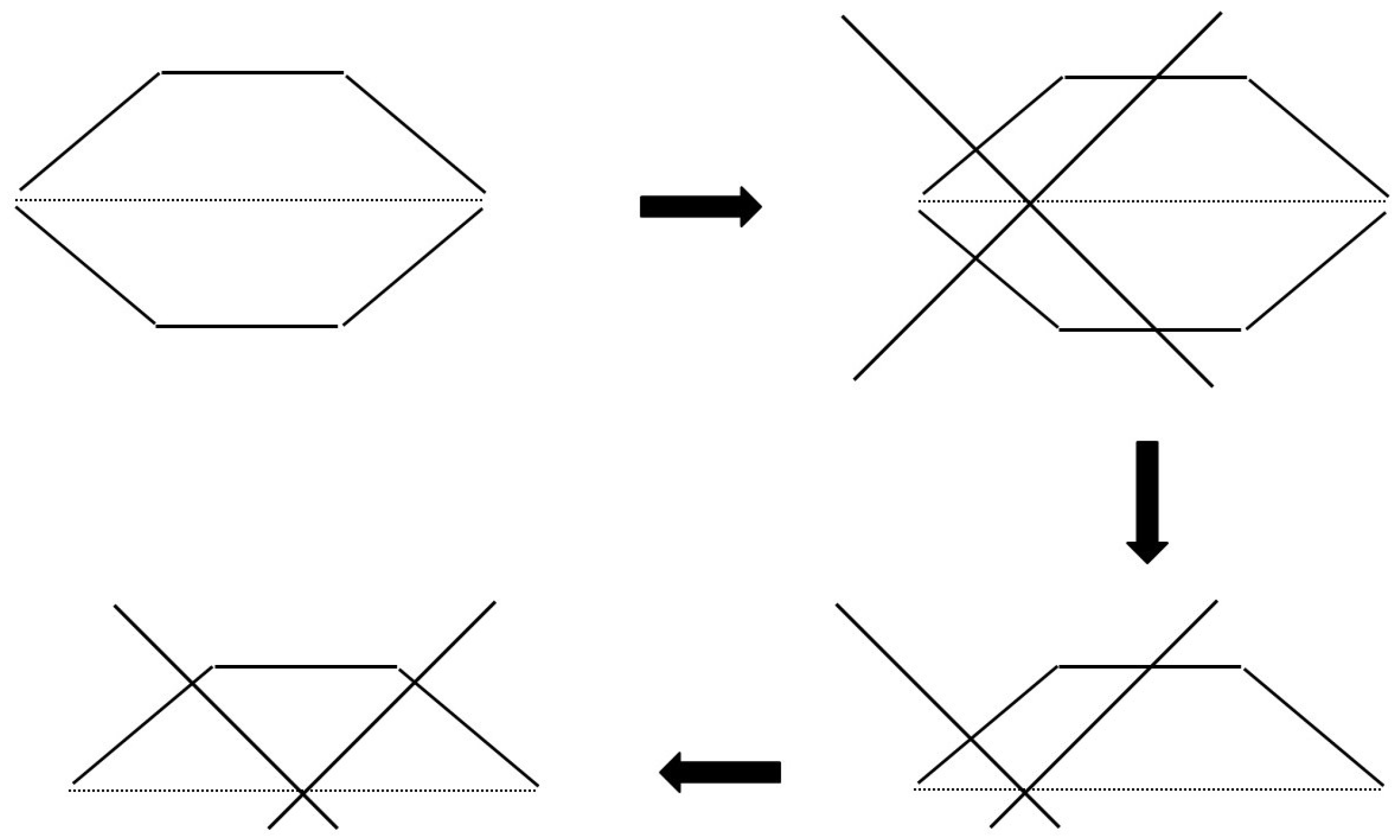
The result is a diamond-shaped polygon spanning $n^k-1$ rows and $n^k+1$ columns. See all the blank cells in Table 12 to visualize this polygon, $P_{old}$. A sketch of $P_{old}$ can be found in the top-left part of Figure 2, where the center row, indexed at ${\displaystyle \frac{n^k}{2}}+1$, is highlighted with a dotted horizontal line.

4.3. Reasoning with Symmetry

We continue with the top-right part of Figure 2. The external user selects the center row of the tableau, which is the longest row in the polygon $P_{old}$, and then chooses an arbitrary cell in that row to place the center of the cutting cross, effectively injecting an arbitrary state symbol, such as $q_5$. Two illustrations are provided in

Table 13. Injecting symbol $q_5$ towards the left in row 9.

1

×

×

×

×

×

×

×

×

$q_0$

×

×

×

×

×

×

×

2

×

×

×

×

×

×

×

×

×

×

×

×

×

×

3

×

×

×

×

×

×

×

×

×

×

×

×

×

4

×

×

×

×

×

×

×

×

×

×

×

×

×

5

×

×

×

×

×

×

×

×

×

×

×

×

×

6

×

×

×

×

×

×

×

×

×

×

×

×

×

7

×

×

×

×

×

×

×

×

×

×

×

×

×

8

×

×

×

×

×

×

×

×

×

×

×

×

×

×

9

×

×

×

$q_5$

×

×

×

×

×

×

×

×

×

×

×

×

×

10

×

×

×

×

×

×

×

×

×

×

×

×

×

×

11

×

×

×

×

×

×

×

×

×

×

×

×

×

12

×

×

×

×

×

×

×

×

×

×

×

×

×

13

×

×

×

×

×

×

×

×

×

×

×

×

×

14

×

×

×

×

×

×

×

×

×

×

×

×

×

15

×

×

×

×

×

×

×

×

×

×

×

×

×

16

×

×

×

×

×

×

×

×

×

×

×

×

×

×

17

×

×

×

×

×

×

×

×

$q_{acc}$

×

×

×

×

×

×

×

×

1

2

3

4

5

6

7

8

9

10

11

12

13

14

15

16

17

and

Table 14. Injecting symbol $q_5$ in the center of row 9.

1

×

×

×

×

×

×

×

×

$q_0$

×

×

×

×

×

×

×

2

×

×

×

×

×

×

×

×

×

×

×

×

×

×

3

×

×

×

×

×

×

×

×

×

×

×

×

4

×

×

×

×

×

×

×

×

×

×

5

×

×

×

×

×

×

×

×

6

×

×

×

×

×

×

×

×

×

×

7

×

×

×

×

×

×

×

×

×

×

×

×

8

×

×

×

×

×

×

×

×

×

×

×

×

×

×

9

×

×

×

×

×

×

×

×

$q_5$

×

×

×

×

×

×

×

×

10

×

×

×

×

×

×

×

×

×

×

×

×

×

×

11

×

×

×

×

×

×

×

×

×

×

×

×

12

×

×

×

×

×

×

×

×

×

×

13

×

×

×

×

×

×

×

×

14

×

×

×

×

×

×

×

×

×

×

15

×

×

×

×

×

×

×

×

×

×

×

×

16

×

×

×

×

×

×

×

×

×

×

×

×

×

×

17

×

×

×

×

×

×

×

×

$q_{acc}$

×

×

×

×

×

×

×

×

1

2

3

4

5

6

7

8

9

10

11

12

13

14

15

16

17

, with the center row indexed as 9. Later, in rows 5 and 13, the user’s interventions will amount to even smaller polygons within the two depicted polygons.

It is unnecessary to treat each of the two smaller polygons inside polygon $P_{old}$ separately. Indeed, given the symmetry of our geometric problem, we may transition from the top-right part to the bottom-right part of Figure 2.

We are now prepared to formally introduce the geometric claims related to a tableau with holes. After performing m cross-cuts in the top half of the original tableau, let $P_{old}$ represent one of the resulting polygons. Now, consider $P_{new}$, a smaller polygon contained within $P_{old}$ formed by introducing an additional cut, bringing the total number of cross-cuts to $m+1$. If at most two rows in $P_{new}$ lack a state symbol, the problem becomes trivial to solve. The analysis in this section focuses on $P_{new}$, assuming it contains at least three rows.

Specifically, we aim to establish the following three claims regarding $P_{old}$ and $P_{new}$, where the relevant measurements are expressed in terms of the number of cells.

Claim 1.

The center row of $P_{new}$ is the longest, yet other rows within $P_{new}$ may be as long.

Remark 9.

We use the symbols H and D to denote, respectively, the length of a horizontal row and the dotted area of a polygon (see, for example,

Table 15. A diamond, consisting of dots and state symbols.

1

$q_0$

2

·

·

·

3

·

·

·

·

·

4

·

·

·

·

·

·

·

5

·

·

·

·

·

·

·

·

·

6

·

·

·

·

·

·

·

7

·

·

·

·

·

8

·

·

·

9

$q_5$

1

2

3

4

5

6

7

8

9

10

11

12

13

14

15

16

17

).

Claim 2.

The length of the center row of $P_{new}$ is at most ${\displaystyle \frac{1}{2}}+{\delta }_1$ times the length of the center row of $P_{old}$, where $-{\displaystyle \frac{1}{2}}\le {\delta }_1\le {\displaystyle \frac{1}{2}}$. That is, $H_{new}\le ({\displaystyle \frac{1}{2}}+{\delta }_1)·H_{old}$.

Claim 3.

We distinguish between a strong Claim 3 and a weak Claim 3:

1.

The total area of $P_{new}$ is at most ${\displaystyle \frac{1}{2}}+{\delta }_2$ times the area of $P_{old}$, where $-{\displaystyle \frac{1}{2}}\le {\delta }_2<0$. That is, $D_{new}\le ({\displaystyle \frac{1}{2}}+{\delta }_2)·D_{old}$.

2.

Filling any hole in the center row of the convex polygon $P_{old}$ of holes scales the space for binary choices within $P_{old}$ by a factor Δ, where $0\le \mathrm{\Delta }<1$.

Remark 10.

The strong claim (1). implies the weak claim (2). as follows:

$$\mathrm{\Delta }={\displaystyle \frac{2·D_{new}}{D_{old}}}\le 1+2·{\delta }_2<1.$$

We shall only rely on the weak claim in Section 5 and simply call this “Claim 3”.

To establish Claims 1–3, we conduct a case analysis in the remainder of this section. We begin with the most symmetric case (Section 4.3.1), proceed to a slightly less symmetric case (Section 4.3.2), and conclude with the least symmetric case (Section 4.3.3). Throughout, we rely on lemmas proved in Appendix B.

In the final case (Section 4.3.3), which encompasses the previous two cases, we are unable to prove the strong version of Claim 3. However, we establish the weak version via a geometric proof in Appendix C, where we take a broader perspective on $P_{old}$. We therefore encourage the reader to view this section as an intuitive buildup to the final case, which naturally leads to the comprehensive proof presented in Appendix C.

4.3.1. The Symmetry-to-Symmetry Transition Case

Rather than immediately analyzing the bottom-right portion of Figure 2, we shift the cut to the middle of the center line, as depicted in the bottom-left portion of Figure 2. Hereby, we examine the most symmetric scenario, specifically when the two state symbols are located in the same column. Readers are encouraged to compare the sketch in the lower left part in Figure 2 with the first nine rows of Table 14.

Transitioning from the top half of Table 14 to Table 15, we observe that the crosses have been removed, with the holes now represented by dots. Collectively, these dots form the convex polygon $P_{new}$.

We define H, the length of the center row of $P_{new}$, as:

$$H=2·N+1,$$

when H is odd, and as:

$$H=2·N,$$

when H is even. For example, in Table 12, we have $N_{old}=8$ and $H_{old}=17$. Similarly, in Table 15, we have $N_{new}=4$ and $H_{new}=9$.

The symmetry of the current case implies that the center row is the longest and that

$$N_{old}=2·N_{new}.$$

Therefore, Claim 1 is automatically confirmed.

Turning to the second claim, we differentiate between the cases where $H_{old}$ is even and where it is odd. In the even case, we would have:

$$H_{new}={\displaystyle \frac{H_{old}}{2}},$$

which would imply ${\delta }_1=0$. In the odd case, we begin with the following:

• $H_{old}=2·N_{old}+1=4·N_{new}+1.$
• $H_{new}=2·N_{new}+1.$
• $H_{new}=({\displaystyle \frac{1}{2}}+{\delta }_1)·H_{old}.$

From these, we derive the equation:

$$2·N_{new}+1=({\displaystyle \frac{1}{2}}+{\delta }_1)·(4·N_{new}+1).$$

Solving for ${\delta }_1$, we find:

$${\delta }_1={\displaystyle \frac{1}{2·(4·N_{new}+1)}}.$$

As $N_{new}\to \infty$, it follows that ${\delta }_1\to 0$. More significantly, as $N_{new}\to 1$, ${\delta }_1\to {\displaystyle \frac{1}{10}}$. This establishes Claim 2.

Next, we define D, the number of cells constituting the polygon, in terms of N and H:

$$D=H+2·\sum _{i=1}^{N-1}(H-2·i).$$

For example, in Table 12, we have

$$D_{old}=17+2·(15+13+11+9+7+5+3)=143.$$

Similarly, in Table 15, we have

$$D_{new}=9+2·(7+5+3)=39.$$

We want to calculate the ratio, ${\displaystyle \frac{D_{new}}{D_{old}}}$, given that

$$N_{old}=2·N_{new},$$

$$H_{old}=4·N_{new}+1.$$

On the one hand, we have:

$$D_{new}=2·N_{new}+1+2·\sum _{i=1}^{N_{new}-1}(2·N_{new}+1-2·i).$$

On the other hand, we can express $D_{old}$ fully in terms of $N_{new}$, as follows:

$$D_{old}=4·N_{new}+1+2·\sum _{i=1}^{2·N_{new}-1}(4·N_{new}+1-2·i).$$

Based on some elementary algebra, we can prove the following two lemmas:

Lemma 2.

$D_{new}=2·N_{new}^2+2·N_{new}-1$.

Proof. 

See Appendix B.    □

Lemma 3.

$D_{old}=8·N_{new}^2+4·N_{new}-1$.

Proof. 

See Appendix B.    □

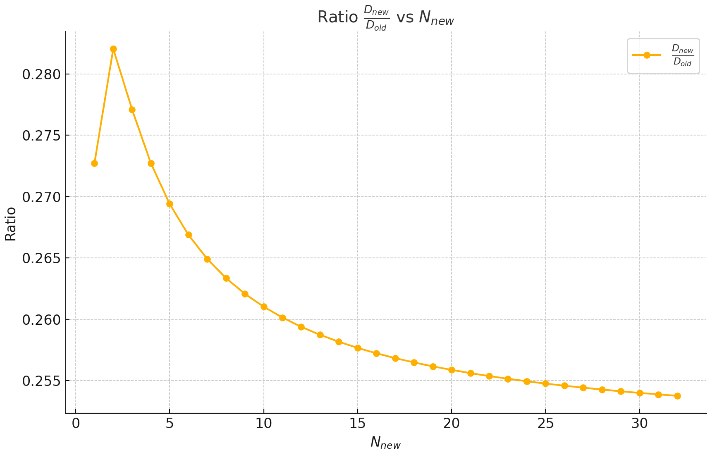
By applying Lemmas 2 and 3, we obtain

$${\displaystyle \frac{D_{new}}{D_{old}}}={\displaystyle \frac{2·N_{new}^2+2·N_{new}-1}{8·N_{new}^2+4·N_{new}-1}}$$

This ratio serves two purposes. First, readers can substitute small values of $N_{new}$ to verify the data points presented in Figure 3. Second, by evaluating the limit of the ratio as $N_{new}\to \infty$, one finds that it is ${\displaystyle \frac{1}{4}}$.

Coming now to an actual confirmation of the third claim, we start thus:

$$D_{new}=({\displaystyle \frac{1}{2}}+{\delta }_2)·D_{old},$$

and we note that as $N_{new}\to \infty$, ${\delta }_2\to -{\displaystyle \frac{1}{4}}$. Also, as $N_{new}\to 1$, we have ${\displaystyle \frac{1}{2}}+{\delta }_2\to 0.273$. More significantly, ${\displaystyle \frac{1}{2}}+{\delta }_2<0.285$ holds for all nonzero values of $N_{new}$. This establishes the strong version of Claim 3.

4.3.2. The Symmetry-to-Skew Transition Case

We now consider the transition from an outer, symmetric polygon $P_{old}$ to a smaller, skewed polygon $P_{new}$, as shown in the bottom-right portion of Figure 2. This transition is further illustrated in the shift from Table 12 to the top half of Table 13.

The three claims can be readily established, as follows:

• Since the larger polygon $P_{old}$ is being cut with two straight lines, each of which is either orthogonal or parallel to $P_{old}$’s longest sides, the longest rows of $P_{new}$ must be situated at the center. The row lengths remain the same or decrease as one moves away from the center toward either the top or the bottom of $P_{new}$. This confirms Claim 1.
• The length of the center row of $P_{new}$ is even shorter than that of the center row in the polygon examined in the previous section (the Symmetry-to-Symmetry Transition Case). Thus, Claim 2 is readily established.
• The total area of $P_{new}$ is even smaller than that of the polygon considered in the previous section. Consequently, Claim 3 is also confirmed.

4.3.3. The Skew-to-Skew Transition Case

We now examine the transition from an outer, skewed polygon $P_{old}$ to a smaller, skewed polygon $P_{new}$. An example of $P_{old}$ is shown in

Table 16. The dots constitute skewed polygon $P_{old}$.

1

$q_0$

2

·

·

·

3

·

·

·

·

·

4

·

·

·

·

·

·

·

5

·

·

·

·

·

·

·

·

·

6

·

·

·

·

·

·

·

·

·

7

·

·

·

·

·

·

·

·

·

8

·

·

·

·

·

·

·

·

·

9

·

·

·

·

·

·

·

·

·

10

·

·

·

·

·

·

·

·

·

11

·

·

·

·

·

·

·

·

·

12

·

·

·

·

·

·

·

·

·

13

·

·

·

·

·

·

·

·

·

14

·

·

·

·

·

·

·

15

·

·

·

·

·

16

·

·

·

17

$q_5$

5

6

7

8

9

10

11

12

13

14

15

16

17

18

19

20

21

, while an example of $P_{new}$ appears, again as a collection of dots, in the top nine rows of

Table 17. A skewed intervention in row 9 with regard to skewed polygon $P_{old}$.

1

$q_0$

2

·

·

·

3

·

·

·

·

×

4

·

·

·

·

×

×

×

5

·

·

·

·

×

×

×

×

×

6

·

·

·

·

×

×

×

×

×

7

·

·

·

·

×

×

×

×

×

8

×

·

·

·

×

×

×

×

×

9

×

×

×

$q_6$

×

×

×

×

×

10

×

×

×

·

·

·

×

×

×

11

×

×

×

·

·

·

·

·

×

12

×

×

×

·

·

·

·

·

·

13

×

×

×

·

·

·

·

·

·

14

×

·

·

·

·

·

·

15

·

·

·

·

·

16

·

·

·

17

$q_5$

5

6

7

8

9

10

11

12

13

14

15

16

17

18

19

20

21

.

Regarding Table 17, note that if symbol $q_6$ is placed in the same column as symbol $q_0$—specifically, in $cell[9,17]$—rather than in column 12, no crosses will appear in row 5, the center row of $P_{new}$. However, in this stringent case, we do have a diamond-shaped polygon $P_{new}$ again. This situation is depicted in

Table 18. A symmetric intervention in row 9 with regard to skewed polygon $P_{old}$.

1

$q_0$

2

·

·

·

3

·

·

·

·

·

4

·

·

·

·

·

·

·

5

·

·

·

·

·

·

·

·

·

6

×

×

·

·

·

·

·

·

·

7

×

×

×

×

·

·

·

·

·

8

×

×

×

×

×

×

·

·

·

9

×

×

×

×

×

×

×

×

$q_6$

10

×

×

×

×

×

×

×

×

·

11

×

×

×

×

×

×

×

×

·

12

×

×

×

×

×

×

×

×

·

13

×

×

×

×

×

×

×

×

·

14

×

×

×

×

×

×

·

15

×

×

×

×

·

16

×

×

·

17

$q_5$

5

6

7

8

9

10

11

12

13

14

15

16

17

18

19

20

21

.

The straight lines of the cutting cross are either parallel or orthogonal to the two longest edges of the skewed polygon $P_{old}$. As a result, the longest rows of $P_{new}$ must be positioned at the center. The row lengths either remain constant or decrease as one moves away from the center toward the top or bottom of $P_{new}$, thereby confirming Claim 1.

Regarding the length of the center row in $P_{new}$, as shown in row 5 in Table 17, we only need to consider the most stringent case, as shown in row 5 in Table 18. We have ${\delta }_1={\displaystyle \frac{1}{2}}$, thereby confirming Claim 2.

Concerning the third claim, we begin by noting that

$$D_{new}+Cross<D_{old}<2·(D_{new}+Cross),$$

where $D_{new}$ denotes all the dots in rows $1-9$ of Table 18 and $Cross$ represents all the crosses depicted in those same rows. $D_{old}$ refers to all the dots in Table 16.

Recall that:

$$H_{new}=2·N_{new}+1,$$

$$D_{new}=2·N_{new}+1+2·\sum _{i=1}^{N_{new}-1}(2·N_{new}+1-2·i).$$

We also have:

$$Cross=2·\sum _{i=0}^{N_{new}-1}(N_{new}-i).$$

In Table 18, we specifically have:

$$N_{new}=4,$$

$$D_{new}=9+2·(7+5+3)=39,$$

$$Cross=2·(4+3+2+1)=20,$$

$$39+20=59<D_{old}<2·59=118.$$

To understand the ratio ${\displaystyle \frac{D_{new}}{D_{old}}}$ in the general case, we express it as follows:

$${\displaystyle \frac{D_{new}}{2·(D_{new}+Cross)}}<{\displaystyle \frac{D_{new}}{D_{old}}}<{\displaystyle \frac{D_{new}}{D_{new}+Cross}}={\left.{\displaystyle \frac{D_{new}}{D_{old}}}\right|}_{\max }.$$

Lemma 4.

$Cross=N_{new}^2+N_{new}$.

Proof. 

See Appendix B.    □

Lemma 5.

From Lemmas 2 and 4, we obtain

$$D_{new}+Cross=3·N_{new}^2+3·N_{new}-1.$$

Proof. 

See Appendix B.    □

From Lemmas 2 and 5, we obtain

$${\left.{\displaystyle \frac{D_{new}}{D_{old}}}\right|}_{\max }={\displaystyle \frac{2·N_{new}^2+2·N_{new}-1}{3·N_{new}^2+3·N_{new}-1}}.$$

As $N_{new}\to \infty$, the ratio ${\displaystyle \frac{D_{new}}{D_{old}}}{|}_{\max }\to {\displaystyle \frac{2}{3}}.$ Some more results are presented in

Table 19. An upper bound on the ratio ${\displaystyle \frac{D_{new}}{D_{old}}}$ in function of $N_{new}$.

${\mathit{N}}_{\mathit{n}\mathit{e}\mathit{w}}$	${\mathit{D}}_{\mathit{n}\mathit{e}\mathit{w}}$	${\left.\frac{{\mathit{D}}_{\mathit{n}\mathit{e}\mathit{w}}}{{\mathit{D}}_{\mathit{o}\mathit{l}\mathit{d}}}\right|}_{\mathbf{max}}$
1	3	0.600
2	11	0.647
3	23	0.657
4	39	0.661
20	839	0.666
30	1859	0.667

. In our running example, this yields:

$${\displaystyle \frac{39}{118}}<{\displaystyle \frac{D_{new}}{D_{old}}}<{\displaystyle \frac{39}{59}}.$$

Alas, these results do not validate the strong version of Claim 3. However, Table 18 does suggest a compensation of crossed-out cells in the lower half of $P_{old}$. This observation, which brings us to the weak version of Claim 3, requires a more comprehensive geometric proof, which is presented in Appendix C.

5. Filling Holes with Backtracking (FHB)

On the one hand, we have assumed the existence of the compact Horn formula ${\psi }_{step}^{\eta }$. On the other hand, we have validated (the weak version of) Claim 3, which asserts that filling any hole in the center row of a convex polygon scales the space for binary choices within the polygon by a factor $\mathrm{\Delta }$, where $0\le \mathrm{\Delta }<1$. With these specifics established, we now turn our attention to filling holes with backtracking (FHB)—an automatable process. Efficiency is achieved by relying on a refined version of the FHB algorithm, as outlined in Section 6.

Conceptually, the FHB algorithm hinges upon the $\mathtt{HORNSAT}$ solver $\mathcal{H}$ and integrates the actions of the external user, automating her interventions and incorporating backtracking as a built-in feature. We stipulate that $\mathcal{H}$ operates in polynomial time. While this polynomial can be replaced by a nearly linear function [9], such details are irrelevant here.

Recall that n is the length of input w. The initial formula ${\psi }_{trim}$,

$${\psi }_{trim}={\psi }_{cell}^{\prime }\wedge {\psi }_{rest}^{\eta }\wedge {\psi }_{extra}^{\eta },$$

is $O\left(n^{{\kappa }_0}\right)$ literals long for some constant ${\kappa }_0$. For example, if ${\psi }_{extra}^{\eta }$ is the longest formula of all three conjuncts, it follows that ${\kappa }_0=4k$, as explained in Section 3.4.

Furthermore, we will have at most $O\left(n^k\right)$ extra stipulations of the form $q@(i,j)$, namely, one per row. Hence, an upper bound on the total cost of our $\mathtt{HORNSAT}$ instance,

$${\psi }_{trim}\wedge q^{*}@(i^{*},j^{*})\wedge \dots ,$$

can be expressed as

$$p\left(n\right)={\kappa }_1·n^{{\kappa }_2},$$

for some constants ${\kappa }_1$ and ${\kappa }_2$.

The FHB algorithm begins with ${\psi }_{trim}$, an instance of size $<p\left(n\right)$, and thus $\le p\left(n\right)$, and runs the solver $\mathcal{H}$ on it, resulting in a trivial “satisfiable” as a tentative outcome. (If N’s computation on w is deterministic, then the outcome is permanent and either satisfiable or unsatisfiable.) Next, the algorithm selects the center row of the tableau and injects the first state symbol q in $Q=\{q_0,q_1,q_2,\dots \}$ into the leftmost hole in that row. If backtracking is required, subsequent iterations will use different state symbols, and if this does not suffice, the next hole (from left to right) in the row will be filled instead, starting again with the first symbol in Q, and so on.

For a row containing holes, there are at most $n^k+1$ ways to inject some specific $q\in Q$ into that row. This leads to our key observation:

There are at most ${\mathsf{c}}_{\mathsf{0}}·(n^k+1)$ ways to inject any $q\in Q$ into a row, where ${\mathsf{c}}_{\mathsf{0}}$ denotes the cardinality of Q.

The first user intervention results in scaling the space of binary choices by $\mathrm{\Delta }$, shrinking from size $\le p\left(n\right)$ to size $\le \mathrm{\Delta }·p\left(n\right)$. In the next two interventions, our algorithm selects the middle row of the first and second convex polygons of holes, read from top to bottom in the tableau. In the next four interventions, our algorithm selects the middle row of each of the four smaller convex polygons of holes, moving sequentially from top to bottom. This pattern continues in subsequent steps.

Immediately after each intervention, the FHB algorithm directs the solver $\mathcal{H}$ to check the entire tableau for unsatisfiability and, in the process, simplify the underlying Horn clauses as much as possible, taking into account all constraints specified by ${\psi }_{trim}\wedge \dots$, where the dots refer to the cumulative intervention stipulations made up to that point.

After each stage of interventions—one intervention in stage 1, two interventions in stage 2, four interventions in stage 3, eight interventions in stage 4, and so on—the solver $\mathcal{H}$ runs on an instance that has been shrunk in size by $\mathrm{\Delta }$. To be technically precise, the solver $\mathcal{H}$ continues operating on the entire instance, but the space of binary choices has been shrunk by a factor of $\mathrm{\Delta }$ after each stage. As a result, we are intrinsically dealing with an instance of size $\le {\mathrm{\Delta }}^m·p\left(n\right)$ after m stages, where $0\le \mathrm{\Delta }<1$. Hence, m is bounded from above by $O\left(log\right(n\left)\right)$. Additionally, the bookkeeping for backtracking itself incurs at most a polynomial cost. A runtime stack with a constant overhead per recursive call is sufficient in practice [11].

Remark 11.

In future work, the engineer could reduce the exponent ${\kappa }_2$ in

$$p\left(n\right)={\kappa }_1·n^{{\kappa }_2},$$

by considering the on-the-fly generation of the Horn constraints associated with either ${\psi }_{extra}^{\eta }$ in Section 3 and/or the constraints associated with ${\psi }_{step}^{\eta }$ in Section 2.3.

For instance, the tailored constraints related to ${\psi }_{extra}^{\eta }$ would be added only when a guess $q^{*}@(i^{*},j^{*})$ is made, causing the formula ${\psi }_{extra}^{\eta }$ to grow incrementally with each additional guess and shrinking during backtracking. Similarly, the formula ${\psi }_{step}^{\eta }$ could expand and contract based on the placement of the q symbols in the tableau, rather than conservatively accounting for all possibilities in advance.

5.1. Recurrence Relation

To analyze the running cost of the FHB algorithm, we set $\mathrm{\Delta }={\displaystyle \frac{1}{2}}$ in conformity with the result proved in Appendix C. We begin by considering the following recurrence relation:

$$T(a·b)={\mathsf{c}}_{\mathsf{0}}·\sqrt{2}·\min (a,b)·T\left({\displaystyle \frac{a·b}{4}}\right)·T\left({\displaystyle \frac{a·b}{4}}\right),$$

where $\min (a,b)$ denotes the smaller of the two lengths, a and b. This relationship is illustrated in Figure 4, a simplified version adapted from Appendix C, specifically for the case $a\le b$.

The recurrence relation expresses that there are $\sqrt{2}·\min (a,b)$ possible positions to place the crossing cut along the dashed horizontal line in Figure 4. When $a\le b$, the parameter c ranges from 0 to $\sqrt{2}·a$, which is equivalent to $\sqrt{2}·\min (a,b)$. Similarly, when $b\le a$, the parameter c ranges from 0 to $\sqrt{2}·b$, again spanning from 0 to $\sqrt{2}·\min (a,b)$. In total, there are ${\mathsf{c}}_{\mathsf{0}}·\sqrt{2}·\min (a,b)$ possible ways to fill a hole in the middle dashed row, where the constant ${\mathsf{c}}_{\mathsf{0}}$ represents the cardinality of the set Q.

The recurrence relation also specifies that the original search space, consisting of $a·b$ cells, is reduced to two smaller, equally sized search spaces of ${\displaystyle \frac{a·b}{4}}$ each. This formulation explicitly excludes scenarios like the following one:

$$T\left({\displaystyle \frac{a·b}{8}}\right)·T\left({\displaystyle \frac{3·a·b}{8}}\right).$$

This exclusion may seem problematic at first. After all, the only requirement we know for certain is that the sum of the two smaller search spaces must equal half of the original search space, since we set $\mathrm{\Delta }={\displaystyle \frac{1}{2}}$ in this discussion. Specifically,

$${\displaystyle \frac{a·b}{8}}+{\displaystyle \frac{3·a·b}{8}}={\displaystyle \frac{a·b}{2}}.$$

Despite this, the exclusion is justified, as we will now explain. In fact, the definition of $T(a·b)$ can be further simplified without loss of generality.

5.2. The Devil’s Advocate

A recurrence relation for the FHB algorithm, regardless of its specific form, must begin with $a=b$, as depicted by the diamond shape in Table 12. During the first user intervention involving the center row of the tableau, the most favorable scenario occurs when the crossing cut is positioned at the leftmost or rightmost edge of the diamond. In either of these two extreme cases, only a single computation path remains, with all other paths discarded from further consideration: the search space is immediately reduced to a single computation path, starting from the top center, passing through either the leftmost or rightmost cell in the middle row, and ending at the bottom center. Conversely, the worst-case scenario arises when the crossing cut is placed exactly halfway along the center row. This results in the formation of two smaller diamond shapes, as illustrated in Table 14.

The devil’s advocate naturally assumes the worst-case scenario at every user intervention. This assumption leads to $a=b$ at each stage of the worst-case run of the FHB algorithm, as illustrated by the transition from Table 12, Table 13 and Table 14. With the invariant $a=b$, the devil’s advocate proposes the following simplified recurrence relation:

$$T\left(a^2\right)={\mathsf{c}}_{\mathsf{0}}·\sqrt{2}·a·T{\left({\displaystyle \frac{a^2}{4}}\right)}^2.$$

Consequently, we change variables with $m=a^2$, as follows:

$$T\left(m\right)={\mathsf{c}}_{\mathsf{0}}·\sqrt{2m}·T{\left({\displaystyle \frac{m}{4}}\right)}^2.$$

Lemma 6.

The dominant behavior of $T\left(m\right)$ is exponential in $\sqrt{m}$. Specifically,

$$T\left(m\right)={\displaystyle \frac{{({\mathsf{c}}_{\mathsf{0}}·{\mathsf{c}}_{\mathsf{1}}·2^{5/2})}^{\sqrt{m}}}{{\mathsf{c}}_{\mathsf{0}}·2^{5/2}·\sqrt{m}}},$$

where constant ${\mathsf{c}}_{\mathsf{0}}$ denotes the size of the state set Q and the constant ${\mathsf{c}}_{\mathsf{1}}=T\left(1\right)$ depends on the size of the tape alphabet Φ.

Proof. 

See Appendix D.    □

Corollary 1.

$$T\left(m\right)\approx C^{\sqrt{m}},$$

with constant $1<C<{\mathsf{c}}_{\mathsf{0}}·{\mathsf{c}}_{\mathsf{1}}·2^5$.

Remark 12.

Corollary 1 is unsurprising, as dividing by 2 instead of 4 (in the recurrence relation) would lead to an exhaustive exploration, as follows:

$$\widehat{T}\left(m\right)={\mathsf{c}}_{\mathsf{0}}·\sqrt{2m}·\widehat{T}{\left({\displaystyle \frac{m}{2}}\right)}^2\approx {\widehat{C}}^m$$

for some constant $\widehat{C}$. A standard derivation is omitted from this paper.

Before running the FHB algorithm, as illustrated by the diamond shape in Table 12, we have the following equation:

$$n^k\times n^k=2·a^2.$$

Again, the scalar 2 arises from $\mathrm{\Delta }={\displaystyle \frac{1}{2}}$.

Now, let $R\left(n\right)$ denote the asymptotic runtime cost of the FHB algorithm. Then, we can express it as:

$$R\left(n\right)\le T\left(a^2\right)=T\left({\displaystyle \frac{n^{2k}}{2}}\right)\approx C^{{\displaystyle \frac{n^k}{\sqrt{2}}}}=2^{(logC)·{\displaystyle \frac{n^k}{\sqrt{2}}}}.$$

Theorem 1.

The runtime $R\left(n\right)$ of the  FHB  algorithm satisfies the upper bound

$$R\left(n\right)\le C^{ϵ·n^k},$$

where $C>1$ is a constant and $ϵ={\displaystyle \frac{1}{\sqrt{2}}}$.

Proof. 

The bound follows from the analysis in the preceding discussion.    □

Theorem 1 suggests a prohibitive asymptotic runtime (with $logC>\sqrt{2}$ in practice). Fortunately, a refinement of the method yields a tighter upper bound.

6. Refining the FHB Algorithm

Even the devil’s advocate will concede that the previous analysis takes an overly pessimistic view by assuming that every cell in the tableau has the potential to contain a (binary) nondeterministic guess. In reality, the situation is far more favorable. Only a small part of the tableau involves binary choices, and more importantly, the outcome of each guess (i.e., the transition to either state $q_a$ or $q_b$) also determines the presence of a specific state symbol (e.g., $q_c$) in a particular cell elsewhere—typically further down—in the tableau.

To see this, let us analyze a 3-SAT solver $N^{*}$. Notably, because any nondeterministic polynomial time Turing machine N (running on some input) can be reformulated in terms of the input for $N^{*}$ with only polynomial overhead, our discussion remains fully general.

Suppose the machine $N^{*}$ runs on an input word w of length n, where w encodes a 3-SAT formula $\varphi$ with l propositional variables ($x_1,\dots ,x_l$) and a number of clauses. Each clause consists of three literals—for example, $x_2\vee \neg x_7\vee x_{92}$.

Remark 13.

We may assume that every variable $x_i$ appears in at least two literals across the formula ϕ; otherwise, such a variable (appearing only once) can be eliminated through preprocessing.

6.1. Coin Tossing

The machine $N^{*}$ stores the encoded formula w on its tape, following the conditions outlined in Section 4.2. During an initial sequence of moves, the tape head shifts to the right, stopping at the first blank symbol immediately following w. The machine then generates l bits, proceeding from left to right and writing each bit—either 0 or 1—into a separate tape cell. This sequence, which is supposed to represent the outcome of l independent coin tosses, is enclosed at both ends by a special marker #.

One outcome of any coin toss must correspond to a rightward movement (+) and the other to a leftward movement (−). To enforce this constraint—consistent with the previous sections in this paper—we implement the following behavior, starting in the ${\widehat{q}}_1$ tossing state:

• If a coin toss yields bit 1, the machine moves its head one cell to the right and re-enters the ${\widehat{q}}_1$ state.
• If a coin toss yields bit 0, the machine first moves its head one cell to the left and enters state ${\widehat{q}}_0$, and then it performs two deterministic moves to the right, ending up in state ${\widehat{q}}_1$ again.

Upon completing this process, the machine will have generated l bits, where the j-th bit ($1\le j\le l$) represents the truth assignment for propositional variable $x_j$. All remaining operations performed by the machine $N^{*}$ are deterministic.

Assigning the truth value 1 to the variable $x_j$ entails that, later on, the machine will set each encoded occurrence of $x_j$ in the word w to 1 and each encoded occurrence of $\neg x_j$ to 0. (A similar remark holds for the truth value 0.) By implementing the proper FHB-procedures, filling holes with state symbols in the coin-tossing section of the tableau will automatically propagate to filling corresponding holes with state symbols in lower sections of the tableau. Moreover, once all l coins have been tossed, the remaining tableau—and therefore the entire tableau—is fully determined. Even the devil’s advocate would expect this property to be reflected in a worst-case analysis of the FHB algorithm or a refinement thereof.

6.2. Four Coin Tosses

Table 20. Tossing four coins from left to right.

1	#	−				#
2	−		−
3		−		−
4			−		−
5		−		·		−
6			−		·
7				−		·
$\mathbf{8}$			−		·
9				−		·
10					−
11				−		·
12					−
13						−
14	#					#
	1	2	3	4	5	6

illustrates the structure of a coin-tossing process for $l=4$. The hyphens and dots in the figure represent potential positions of the tape head (i.e., state symbols), with the distinction between the two serving only for visual clarity. The two extreme computation runs are depicted solely with hyphens: the diagonal run at the top (consisting of five hyphens) produces all four bits as 1, while the zigzagging run takes longer to complete and results in all four bits being 0.

Specifically, the hyphen in $cell[1,2]$ means that the cell contains the symbol pair ${\displaystyle \frac{\square }{{\widehat{q}}_1}}$. Elsewhere in this paper, we represent this pair as

$${\widehat{q}}_1\square$$

which occupies two cells instead of one. These notational variations are inconsequential and can be regarded as equivalent.

As Table 20 illustrates, the coin-tossing process is represented by a table with $3l+2$ rows and $l+2$ columns. This table can be embedded within a $(3l+2)\times (3l+2)$ mini tableau—and more generally, within a $(\kappa ·l)\times (\kappa ·l)$ mini tableau, for some constant $\kappa$. The recurrence relation and Theorem 1 in Section 5.2 apply to this mini tableau.

Now, if the 3-SAT solver $N^{*}$ were solely responsible for tossing l coins, no further improvement in the worst-case runtime of the FHB algorithm would be possible. In reality, however, the tossed coins are made to correlate through the word w, which encodes the 3-SAT formula $\varphi$. For not all sequences of l coin tosses are valid—if any at all.

6.3. Properties of Computation

Appreciating that there is a correlation between the tosses amounts to recognizing the following two properties regarding the computation runs of $N^{*}$ on w:

• The mini tableau captures all nondeterminism (coin tossing) inherent to $N^{*}$, while also including subsequent deterministic computations.
  • Example 1: If four 1 bits are tossed consecutively, $N^{*}$’s tape head lands on $cell[5,6]$ of Table 20 and immediately begins deterministic computation from row 6.
  • Example 2: If four 0 bits are tossed instead, $N^{*}$ uses almost the entire mini tableau to complete the coin tossing, reaching $cell[13,6]$, before starting deterministic computation in rows 14 onward.
• The subsequent deterministic computation does not revisit column 6 or any column to its right. See Table 20. More generally, the rightmost column of the mini tableau, which is of length $O\left(l\right)$, contains exactly one state symbol (namely, ${\widehat{q}}_1$).

  (a)

  Although the two hyphens and three dots in column 6 of Table 20 indicate multiple possible positions for a state symbol, only one state symbol can appear in any given computation. (Moreover, that symbol must be ${\widehat{q}}_1$.)

  (b)

  For each input formula $\varphi$ and each placement of ${\widehat{q}}_1$ in the rightmost column, we can determine (and thus preprogram) the position of the machine’s head—though not its state—in every subsequent row of the entire tableau. In other words, except for a significant portion of the mini tableau, every row of the tableau consists of a single empty cell with all other cells filled by crosses.

6.4. A Conservative but Insightful Theorem

Our thought experiment—initiated by the hypothesis that the compact Horn formula ${\psi }_{step}^{\eta }$ exists—combined with Theorem 1 from our initial cost analysis leads to a refined version of the FHB algorithm. This improved algorithm (rFHB) relies on the two properties discussed above. We introduce rFHB in the proof of the following theorem:

Theorem 2.

The runtime of rFHB, a refined version of the FHB algorithm, is bounded from above:

$$R\left(n\right)\le K^{f(n,k)},$$

where K is a constant and

$$f(n,k)\approx {\left({\displaystyle \frac{n^{2k}}{4}}\right)}^{{\displaystyle \frac{1}{3}}}={\displaystyle \frac{n^{\frac{2k}{3}}}{1.59}}.$$

Remark 14.

Arguably, we even have:

$$f(n,k)\approx {\left({\displaystyle \frac{n^{2k}}{8}}\right)}^{{\displaystyle \frac{1}{4}}}={\displaystyle \frac{n^{\frac{k}{2}}}{1.68}}.$$

• Proof Outline

Suppose $N^{*}$ runs in $n^k$ time. (Typically, $k=2$ for an unsophisticated 3-SAT solver, and $k=1$ otherwise.) Consider the corresponding $n^k\times n^k$ tableau. Based on the above discussion, we can refine the original $\mathtt{FHB}$ algorithm as follows:

• Guess a row $\widehat{r}$ such that ${\widehat{q}}_1@(\widehat{r},\widehat{c})$ holds, where $\widehat{c}$ is the index of the rightmost column in the mini tableau—with $\widehat{c}=6$ in Table 20.
  • The guess results in crossing out many cells in the remainder of the tableau, as described previously in item $2\left(b\right)$.
  • The associated cell crossings are revoked when backtracking from the guess.
• Let the original $\mathtt{FHB}$ algorithm operate in the $(3l+2)\times (3l+2)$ mini tableau, yet in adherence to guess ${\widehat{q}}_1@(\widehat{r},\widehat{c})$, starting with the center row of that mini tableau. (Take one of the two center rows when $3l+2$ is even).
• For each state symbol injected by the $\mathtt{FHB}$ algorithm within the mini tableau, now also inject the corresponding state symbols outside the mini tableau (within the $n^k\times n^k$ tableau).
• Backtracking in the $\mathtt{FHB}$ algorithm triggers backtracking of the corresponding state symbols injected outside the mini tableau.

The inferences from state symbols inside to outside the mini tableau must be pre-programmed. For example, if coin $x_2$ has been tossed to 1 early in the tableau, then—due to the preprogramming—the propagation’s state symbol (used when updating $x_2$’s truth value in w) is already known, deep down in the tableau. (Recall Remark 13 to grasp the underlying structure at work. After the coin-tossing stage—mostly beyond the confines of the mini tableau—the machine propagates the truth value of each propositional variable to the encoded 3-SAT formula w on the tape’s left side.)

A minor caveat is that, for any coin index j (where $1\le j\le l$), there are $O\left(l\right)$ ways to specify that coin $x_j$ was tossed to 1 (or alternatively, to 0). For instance, coin $x_2$ in Table 20 can land on 1 in two ways:

$${\widehat{q}}_1@(3,4)\vee {\widehat{q}}_1@(5,4).$$

Each such case requires the symbol $q_{sat}$ to be activated in a predetermined cell $c_{*}$ further down in the tableau:

$$\left({\widehat{q}}_1@(3,4)\to q_{sat}@c_{*}\right)\wedge \left({\widehat{q}}_1@(5,4)\to q_{sat}@c_{*}\right),$$

where the contents of cell $c_{*}$ encode the state of $N^{*}$ after scanning the first clause containing the literal $x_2$.

Remark 15.

If multiple clauses in ϕ contain the literal $x_2$, analogous Horn implications apply to each such clause. The total number of Horn constraints scales polynomially with l and the number of clauses in ϕ. Note: $q_{sat}$ and $q_{accept}$ are distinct state symbols.

For a conservative cost analysis of the $\mathtt{rFHB}$ algorithm, it is important to note that the free hole-filling outside the mini tableau occurs in an area at least as large as the mini tableau. This implies that, at the very least, $\mathrm{\Delta }={\displaystyle \frac{1}{4}}$ rather than ${\displaystyle \frac{1}{2}}$. Consequently, we solve the following recurrence relation:

$$T\left(m\right)={\mathsf{c}}_{\mathsf{0}}·\sqrt{2m}·T{\left({\displaystyle \frac{m}{8}}\right)}^2\approx K^{m^{{\displaystyle \frac{1}{3}}}},$$

for some constant K. Finally, by substituting ${\displaystyle \frac{n^{2k}}{4}}$ for m, we obtain the result:

$$K^{f(n,k)},$$

with

$$f(n,k)\approx {\left({\displaystyle \frac{n^{2k}}{4}}\right)}^{{\displaystyle \frac{1}{3}}}={\displaystyle \frac{n^{\frac{2k}{3}}}{1.59}}.$$

Remark 16.

While overly conservative, Theorem 2 with the exponent $f(n,k)$ already demonstrates genuine compression compared to Theorem 1. Furthermore, if we set $\mathrm{\Delta }={\displaystyle \frac{1}{8}}$—a choice the devil’s advocate might readily accept—the exponent of m decreases further from ${\displaystyle \frac{1}{3}}$ to ${\displaystyle \frac{1}{4}}$, which leads to the improved definition of $f(n,k)$ in Remark 14. The iterative application of the rFHB algorithm will be discussed in a forthcoming article.

7. Conclusions

In this paper, we depart from the classical top-down interpretation of a nondeterministic computation of N on an input w of length n, which runs in at most $n^k$ steps. In the worst case, this classical approach requires making a binary choice at each step, resulting in a deterministic time complexity of essentially $2^{n^k}$. Instead, we abstract away the complexity of enforcing N’s step-by-step behavior, hypothesizing that it can be succinctly represented by a Horn formula ${\psi }_{step}^{\eta }$.

As a result, our focus shifts to a timeless tableau (with approximately $n^k$ rows and $n^k$ columns), in which the contents of each cell must be guessed. Now, we have increased the deterministic time complexity to $2^{n^{2k}}$. However, by leveraging a compression result related to the tableau and the behavior of the Turing machine’s head within it (recall formula ${\psi }_{extra}^{\eta }$, which leads to $\mathrm{\Delta }={\displaystyle \frac{1}{2}}$ in Claim 3), we significantly reduce the search space. This ultimately results in a deterministic time complexity that is only slightly worse than the classical $2^{n^k}$ result (see Theorem 1).

Next, we distinguish between a pure coin-tossing machine, to which the previously discussed time complexities apply, and an actual 3-SAT solver—a nondeterministic polynomial time Turing machine $N^{*}$ that generates not truly random bits but rather correlated bits. In other words, the computational behavior of $N^{*}$ within a tableau can be further compressed, achieving a reduction factor of at least $\mathrm{\Delta }={\displaystyle \frac{1}{4}}$ instead of $\mathrm{\Delta }={\displaystyle \frac{1}{2}}$, leading to a strong compression result (Theorem 2). In future work, we will apply this result iteratively.

The core idea behind $\mathrm{\Delta }={\displaystyle \frac{1}{2}}$ can be summarized as follows. Consider an $n^k\times n^k$ tableau, initially empty. By selecting two specific cells, $c^{*}$ above and $c_{*}$ multiple rows below, where N’s head should be located, we can force a binary choice to collapse into a deterministic move. This contrasts with the scenario where only one of these cells is filled with a state symbol, or where two nearby cells are each filled with a state symbol, allowing for greater nondeterminism. Specifically, if only the top cell, $c^{*}$, is filled with a state symbol, the machine can move both left and right. However, if a second cell, $c_{*}$, is filled at an extreme relative position later in time, various movements earlier in time become restricted—only several rightward moves, for instance, remain feasible for the machine to go from cell $c^{*}$ to the lower cell $c_{*}$.

To further improve the reduction factor from $\mathrm{\Delta }={\displaystyle \frac{1}{2}}$ to $\mathrm{\Delta }={\displaystyle \frac{1}{4}}$, we leverage the fact that the nondeterministic Turing machines involved in $\mathcal{NP}$ computations are not pure coin-tossing machines. Instead, their state transitions exhibit structured dependencies across the tableau. For instance, if the state symbol in cell $c^{*}$ indicates that the machine has just tossed the second coin to 1 (in one of multiple ways) and is about to toss the third coin, this constrains the state symbol in a later cell $c_{*}$. Due to several dependencies—embedded in the tableau’s deterministic substructure—the machine may then be forced to toss the next coin to 1 rather than 0. This long-range interaction preserves the computation’s satisfiability, though the underlying mechanism is very subtle. Crucially, $N^{*}$’s computation on w does not develop top-down but grows in an interleaved fashion across the tableau’s rows.

To recapitulate, an accepting tableau provides a framework for demonstrating the satisfiability of $\psi$, confirming that the nondeterministic polynomial time Turing machine N accepts the input word w. The propositional formula $\psi$ consists of two components: ${\psi }_{cell}$ and ${\psi }_{rest}$, both in 3cnf. Since ${\psi }_{rest}$ appears more challenging for satisfiability, this raises the question of whether distinguishing between 3cnf and 2cnf for ${\psi }_{cell}$ is consequential. In this paper, we have proven that if ${\psi }_{rest}$ can be compactly represented as a Horn formula, the gap between 3cnf and 2cnf for ${\psi }_{cell}$ becomes small: $\psi$ can be satisfied efficiently in $K^{f(n,k)}$ steps, with $f(n,k)\approx n^{{\displaystyle \frac{2}{3}}k}$, where N operates in $O\left(n^k\right)$ steps and both k and K are constants.