Scalable Graph Coloring Optimization Based on Spark GraphX Leveraging Partition Asymmetry

Abstract

Many challenges in solving large graph coloring through parallel strategies remain unresolved. Previous algorithms based on Pregel-like frameworks, such as Apache Giraph, encounter parallelism bottlenecks due to sequential execution and the need for a full graph traversal in certain stages. Additionally, GPU-based algorithms face the dilemma of costly and time-consuming processing when moving complex graph applications to GPU architectures. In this study, we propose Spardex, a novel parallel and distributed graph coloring optimization algorithm designed to overcome and avoid these challenges. We design a symmetry-driven optimization approach wherein the EdgePartition1D strategy in GraphX induces partitioning asymmetry, leading to overlapping locally symmetric regions. This structure is leveraged through asymmetric partitioning and symmetric reassembly to reduce the search space. A two-stage pipeline consisting of partitioned repaint and core conflict detection is developed, enabling the precise correction of conflicts without traversing the entire graph as in previous algorithms. We also integrate symmetry principles from combinatorial optimization into a distributed computing framework, demonstrating that leveraging locally symmetric subproblems can significantly enhance the efficiency of large-scale graph coloring. Combined with Spark-specific optimizations such as AQE skew join optimization, all these techniques contribute to an efficient parallel graph coloring optimization in Spardex. We conducted experiments using the Aliyun Cloud platform. The results demonstrate that Spardex achieves a reduction of 8–72% in the number of colors and a speedup of 1.13–10.27 times over concurrent algorithms.

1. Introduction

The Vertex Graph Coloring Problem (VGCP) is a fundamental issue in graph theory that involves assigning colors to vertices such that no adjacent vertices share the same color. In practical applications, the VGCP arises in any domain in which mutually conflicting entities must be assigned distinct labels, such as frequency allocation in wireless networks, register assignment in compilers, and task scheduling in parallel systems [1,2]. However, real-world graphs, whether drawn from social media, biological interaction networks, or transportation infrastructures, rarely exhibit perfect symmetry. Instead, they feature skewed degree distributions, irregular community boundaries, and heterogeneous subgraph densities. Such asymmetries degrade the solution quality of coloring heuristics and hinder their scalability in large-scale and distributed settings [3]. Moreover, the exact computation of chromatic numbers is NP-complete [4], forcing practical algorithms to trade optimality for tractability. In distributed and cloud computing environments, naive strategies that assume graph symmetry typically fail: either executors stall during conflict resolution, or the number of colors must be increased to maintain throughput [3,5]. As demonstrated by Jones and Plassmann (1993) [1], existing algorithms must accept either higher color usage to speed up execution or longer runtimes to reduce the chromatic number [3,5,6,7].

Classical VGCP approaches have relied on sequential heuristics such as greedy degree ordering, DSATUR, and related local-search techniques, which perform adequately on graphs of moderate size but do not extend to problems encompassing millions or billions of edges [3]. To overcome this limitation, Pregel-like systems (for example, Apache Giraph) adopt superstep synchronization and bulk data exchange; nevertheless, they incur substantial overhead when resolving color conflicts across partitions, since neighboring subgraphs may require serialized repair operations [6,7,8]. More recent GPU-based implementations exploit fine-grained parallelism to reduce the number of coloring iterations and offload computation-intensive kernels to specialized hardware [5,9,10,11], but these solutions remain constrained by GPU memory limits and the cost of transferring border-region data.

Contemporary Big Data platforms such as Hadoop, Spark, and Flink furnish robust fault tolerance and in-memory processing that facilitate large-scale graph partitioning and local coloring [7,12,13]. Nonetheless, three key challenges remain, each rooted in the asymmetry of real-world graphs: (1) partition-induced conflicts, where replicated vertices across subgraphs force expensive global coordination; (2) load imbalance, as asymmetrically distributed high-degree vertices overburden some executors while others remain underutilized; and (3) data-management pressure, as shuffling large edge and vertex sets provokes I/O bottlenecks and undermines parallel efficiency [4,8,14,15].

The above trade-offs and challenges posed by structural asymmetry directly inform the design of the method we propose. In this study, we propose Spardex, a novel parallel and distributed graph coloring algorithm designed for large-scale VGCP instances and implemented using Spark GraphX configured on top of the Hadoop YARN resource scheduler. Previous studies using Pregel-based frameworks [5,6] incur substantial coordination overhead due to sequential global correction stages; in contrast, our method eliminates the need for a global traversal through enabling each partition to be independently colored and to resolve conflicts in parallel by focusing only on repeated key conflicts. GPU-based solutions suffer from memory bottlenecks and limited graph size scalability [5,9,10,11], whereas our method leverages in-memory distributed processing to handle billion-edge graphs without specialized accelerators, maintaining low color usage and high convergence efficiency. The principal contributions of our study are as follows:

(1)

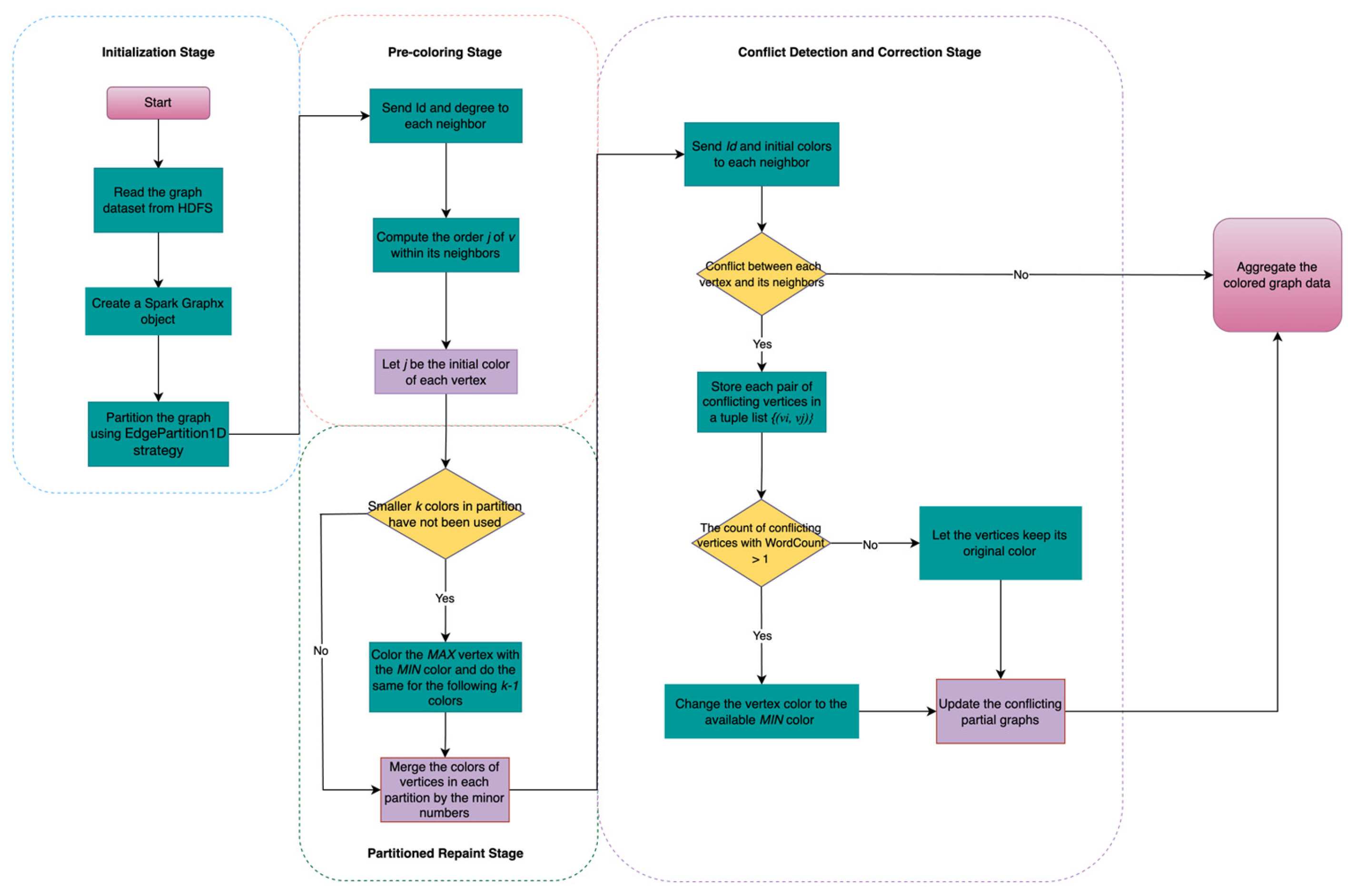
Symmetry-aware EdgePartition1D initialization: The input graph is loaded into GraphX and partitioned using the EdgePartition1D strategy. Within each partition, vertices are pre-colored according to local degree ranking. This produces a high-quality initial configuration that accounts for inherent structural symmetries and effectively manages regions of high structural density arising from asymmetry.

(2)

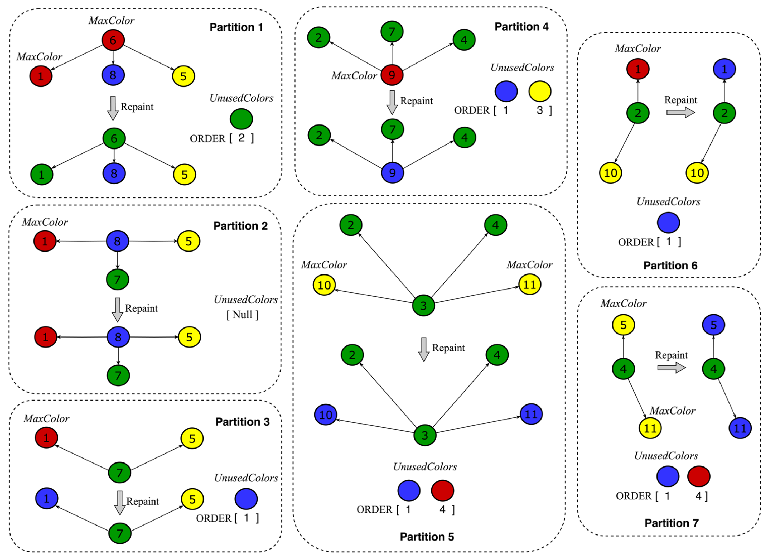
Partitioned repaint stage: Each partition independently reassigns its vertices to the smallest available colors in parallel, obviating costly global iterations and substantially curtailing inter-partition messaging.

(3)

Minimum-based merge for boundary resolution: Vertices spanning multiple partitions exchange only the minimal valid color in localized merge operations, thereby avoiding full-graph synchronization.

(4)

Two-stage MapReduce conflict detection and correction pipeline: A concluding Spark MapReduce job enumerates residual conflicts and applies targeted corrections in a single pass over the conflict set, ensuring convergence without traversing the entire graph.

The rest of this study is organized as follows: Section 2 explores the parallelism limitations of existing graph coloring algorithms and outlines the motivation for this research. Section 3 presents the design of the algorithm. Section 4 discusses the optimization strategies for memory management and computational efficiency. Section 5 evaluates the overall performance of Spardex. Finally, Section 6 concludes the study and outlines future research opportunities.

2. Motivation

This section reveals the principal limitations of existing methods based on Pregel-like frameworks in large-graph coloring, which motivated us to develop Spardex.

According to previous studies [1,7,10,13], the coloring process of graph coloring algorithms on Pregel-like frameworks can be divided into two stages: the pre-coloring stage and the conflict detection and correction stage. Each of these stages serves a distinct purpose: the former specifies a method to assign an initial color to each vertex, while the latter detects and corrects color conflicts between neighboring vertices.

As the calculation methods used in the pre-coloring stages of different works vary significantly, we used the comprehensive DistG [7] algorithm as an example. We chose DistG as our primary case study for two reasons. First, DistG exemplifies a comprehensive integration of degree-based pre-coloring and iterative local refinement within a single framework, making it representative of state-of-the-art Pregel implementations. Its design has been evaluated on both directed citation networks and undirected social graphs, demonstrating robust performance across network types and degree distributions. Second, the powerful underlying computing framework used for data storage and graph computing in DistG, Hadoop, is widely used in social platforms. This serves as a valuable reference for our development of a new algorithm based on Spark GraphX on top of Hadoop.

The core concept of the pre-coloring stage in DistG is to define the order of each vertex among its neighbors, calculated based on its degree and the degrees of its neighbors—vertices with larger degrees receive smaller initial colors. As highlighted by Gebremedhin et al. [16], this approach prioritizes high-degree vertices, aiming to reduce conflicts and minimize the overall number of colors used. However, pre-coloring methods vary significantly across algorithms, making it difficult to standardize or optimize this phase across frameworks.

We now walk through the DistG pre-coloring stage by applying it to the graph in Figure 1a; we discuss the method’s shortcomings later. The process is as follows:

Step 1: Determine the degree and identifier ($Id$) of each vertex, $v$, and spread to all its neighbors.

Step 2: Calculate the order, $j$, of each $v$ according to its degree within all its neighbors; as noted, the larger the degree, the smaller the order. When the degrees are equal between several vertices, the comparison is defined based on their $Id$s—the larger the $Id$, the smaller the order. Thus, vertex 8 has order 1; vertices 2, 3, 4, and 7 have order 2; vertices 5, 10, and 11 have order 3; and the rest have order 4.

Step 3: Define the initial color of each $v$ corresponding to its $j$. As shown in Figure 1b, each vertex takes its initial color, which is sorted as color 1 (blue), color 2 (green), color 3 (yellow), or color 4 (red).

Figure 1. A graph example. (a) Uncolored original graph; (b) running example of the pre-coloring stage of the DistG algorithm.

Figure 1. A graph example. (a) Uncolored original graph; (b) running example of the pre-coloring stage of the DistG algorithm.

The pre-coloring stage of DistG is an efficient approach, attempting to color all vertices in one stage and resolving conflicts only in subsequent steps, significantly reducing execution time. This degree-based sorting method reduces the number of color conflicts by assigning colors to high-degree vertices first, allowing low-degree vertices to be colored with minimal conflict afterward. Since high-degree vertices have more neighbors, assigning colors to them first reduces color conflicts more effectively, thus improving the overall efficiency of the algorithm. We now examine a potentially better solution, as illustrated in Figure 2.

Figure 2 illustrates a superior coloring solution that utilizes three colors for the entire graph, requiring fewer in the pre-coloring stage. This observation motivates the development of a new pre-coloring method with a smaller chromatic number, enabling the entire graph coloring algorithm to use fewer colors, thus improving efficiency and reducing computational complexity.

The conflict correction stage is another critical phase in parallel graph coloring algorithms. As noted by Gandhi and Misra [13], conflict correction accounts for most of the execution time in these algorithms, making parallelization in this stage crucial for overall performance. To quantify the parallelism of the conflict correction stage, we define the metric $P$ as the number of vertices processed per second in a distributed environment. Let $v.num$ denote the total number of vertices requiring conflict correction and $T_c$ represent the execution time (in seconds) of the conflict correction phase. Parallelism, $P$, is calculated as $P= {\displaystyle \frac{v.num}{T_c}}$. This metric reflects the algorithm’s ability to process vertices concurrently across distributed nodes. A higher $P$ indicates stronger parallel scalability, as more vertices are resolved per unit time.

We conducted this experiment on a cluster comprising 1 master node and 10 slave nodes. Each node was equipped with an Intel(R) Core i7 processor (16 cores, 5.2 GHz) and 32 GB of RAM, running Ubuntu 16.04.7 LTS with Hadoop version 3.2.4. We compared the parallelism of the conflict correction stage of the DistG algorithm against a baseline that represents the maximum theoretically achievable parallelism on this Hadoop cluster. The experimental results are illustrated in Figure 3.

The experimental results show a significant parallelism gap between DistG’s color correction stage and the baseline, especially for large, complex graphs. Zheng et al. and Che et al. [10,11] found that purely sequential conflict correction limits parallelism. To address this, we propose a hybrid approach that dynamically adjusts parallelism based on conflict complexity for optimal performance.

3. Algorithm Design

This section presents our design philosophy and describes the Spardex algorithm.

3.1. Design Philosophy

We have clarified the main problems with existing algorithms: (a) the vertex coloring method in the pre-coloring stage does not effectively minimize the chromatic number, and (b) the conflict detection and correction stage fails to fully leverage the parallel and distributed computing capabilities of Pregel-like frameworks.

These limitations suggest that previous methods fail to fully leverage local symmetries in graph structure while lacking mechanisms to cope with topological asymmetries across partitions. This study addresses these two challenges by proposing a highly parallel algorithm within the Spark GraphX framework. The core approach involves partitioning the uncolored graph into subgraphs at the physical level and then applying a novel strategy to repaint vertices within different partitions after computing their initial colors. The subgraph merging process follows a “minor-number-first” strategy, modifying the graph’s topology to resolve conflicts efficiently. Rather than traversing the entire graph as in previous methods, our algorithm focuses exclusively on repeated key conflicts, significantly improving conflict resolution efficiency and overall performance [7,12,13].

Spardex begins by creating a GraphX object and partitions the graph into subgraphs using the EdgePartition1D strategy, a design choice closely aligned with GraphX’s edge-centric execution semantics and memory layout. Specifically, EdgePartition1D introduces a topological asymmetry by assigning edges solely based on their source vertices, leading to partitions that are non-overlapping on edges but partially overlapping on vertices [13]. Instead of attempting to mitigate this asymmetry, Spardex strategically exploits it. The repaint-and-merge scheme is inherently designed for non-uniform vertex distributions, facilitating localized conflict resolution and thereby enhancing both efficiency and scalability in distributed execution [17].

3.2. Spark-Based Graph Coloring Algorithm

The coloring process begins with a Spark application that operates on the Hadoop YARN resource scheduler and HDFS file system. The graph topology datasets are stored in HDFS and subsequently loaded into a GraphX object for coloring. The Spark-based graph coloring algorithm is outlined in Algorithm 1.

Algorithm 1. Spardex: a high-parallelism graph coloring algorithm

Require: Graph, $G$; $PartitionNum$ Ensure: Graph coloring plan, $COLORS$; and the colors $chromatic\_num$ used for coloring graph $G$; 1: function $ComputeOrder$(Vertex, $v$; message, $m$) 2:   $max$ ← the_biggest_vertexId($G$) 3:   for ($v.Id$ = 1; $v.Id$ < $max$; $v.Id$ ++) 4:    for (message: $m$) do 5:        $j_v$ ← 1; 6:     if ($d_v$ < $d_u$) $\vee$ (($d_v$ = $d_u$) $\wedge$ ($v.Id$ < $u.Id$)) $j_v$ ++; 7: end function 8: function $PartitionedRepaint$($Unusedcolor\_num$, $k$) 9:   k ← 0; $v_{max}$ ← $patition.vertices\_num$; 10:    for (partition = 0; partition < $Partition\_num$; partition++) 11:      for ($color$ = $MaxColor-1$; $color$ > 0; $color$ - -) 12:        if ($color$ $\notin$ $partition.colors$) 13:         stack $Unusedcolors$ ← $color$; 14:         $k$ ++; 15:     if ($Unusedcolors$ == $\varnothing$) return 0; 16:     else for ($color$ = $Unusedcolors.top$; $color$ > $Unusedcolors.bottom$; $color$ - -) 17:        pull ($Unusedcolors.top$); 18:        $MaxColor$ ← $Unusedcolors.top$; 19:      for ($v$ = 1; $v$ < $v_{max}$; $v$ ++) 20:        while ($partition.color\left(v\right)$) $color\left(v\right)$ ← $partition.color\left(v\right).\mathrm{m}\mathrm{i}\mathrm{n}( )$; 21: end function 22: function $ConflictCountAndCorrection$(Tuple, $T$) 23:  for ($v.Id$ = 1; $v.Id$ < $max$; $v.Id$ ++) 24:    if ($color\left(v\right)$ == $color(v.neighbor)$) 25:      $T$ ← Tuple ($v$, $v.neighbor$); 26:  $DuplicateRemoval$($T$); 27:  $count$ ← $ConflictCount$($T$);  $keyconflicts$ ← $count$.filter (. _ > 1) 28:  while ($keyconflicts$) do in parallel: $ConflictCorrection$($v$) 29: end function

In Spardex, we maintain a read-only color array accessible to all Spark executors, denoted by $COLORS$. The vertex ordering follows the same mathematical method as DistG [7], prioritizing degree-based ordering [16,18] (for details, see [7]). The partitioned repaint stage begins after assigning initial colors to vertices in parallel. Each partition identifies the smallest $k$ unused colors from $MaxColor-1$ to $Color 1$, storing them in a read–write stack, $Unusedcolors$. If $Unusedcolors$ is empty, no repainting occurs; otherwise, vertices with $MaxColor$ are reassigned to the smallest available color, and the remaining $k-1$ colors are similarly distributed [12].

Since vertices may receive different colors across partitions, we resolve inconsistencies using a minor-number-first strategy. This alters the graph’s topology, enabling conflict resolution by correcting only repeated key conflicts rather than traversing the entire graph [6], which we will prove it.

• Initial Conditions and Repainting Strategy

Assume that the graph, $G$, is divided into $k$ subgraphs, and the vertices in each subgraph are independently recolored. For each subgraph, we recolor the vertex with the maximum color to the smallest unused color. This strategy aligns with heuristic methods commonly used in parallel graph coloring algorithms [1,3,7,13,19,20]. Additionally, Vizing’s theorem [21] provides theoretical support for estimating the chromatic number of a graph.

$$\forall v_i \in P_j, c\left(v_i\right)=\min \left\{c\left(v\right) \right| v \in P_j, c\left(v\right) is unused\}$$

(1)

where $P_j$ denotes the $j$th subgraph, and $c\left(v_i\right)$ represents the color of vertex $v_i$. This process ensures that the color allocation within each subgraph is locally optimal.

2.

Definition of Conflict Vertices

Two vertices, $u$ and $v$, conflict if $c\left(u\right)=c\left(v\right)$ and $u$ and $v$ are adjacent. This definition can be supported by relevant theories in graph theory [6,22,23]. In this case, an edge $(u, v)$ is added to the conflict graph, $G_c$:

$$G_c=\left\{\left(u, v\right) \right| c\left(u\right)=c\left(v\right), \left(u, v\right) \in E\left(G\right)\}$$

(2)

where $E\left(G\right)$ represents the edge set of graph $G$.

3.

Critical Conflict Vertices

The conflict counting, $w_c\left(v\right)$, of a vertex, $v$, is defined as the number of times it appears in a conflict. If $w_c\left(v\right) >1$, then $v$ is a critical conflict vertex. This definition is closely related to the complexity of handling conflicts during graph partitioning [3,14,24]:

$$w_c\left(v\right)= {\sum }_{u \in N\left(v\right)}1\{c\left(u\right)=c(v\left)\right\}$$

(3)

where $N\left(v\right)$ is the neighborhood set of vertex $v$, and $1\{·\}$ is the indicator function.

4.

Assumption of No Critical Conflict Vertices

Assume there is a pair of conflicting vertices, $u$ and $v$, such that $w_c\left(u\right)=1$ and $w_c\left(v\right)=1$. In other words, there is a conflict between $u$ and $v$, but each vertex is in conflict only with the other. This assumption can be supported by strategies for conflict handling in distributed graph coloring [23,24,25].

5.

Analysis After Repainting Within the Partition

After repainting within the partition, assume that vertices $u$ and $v$ are in the same partition and have the same initial color. According to the intra-partition repainting strategy, the vertex with the maximum color is recolored to the smallest unused color, and all vertices are processed sequentially. Similar strategies [2,26] have been applied in solving the independent set problem, and parallel graph processing methods [14,25] in selective scheduling also support this process.

Case of a Single Conflict Vertex: If there is a conflict between $u$ and $v$, but each vertex is in conflict only with the other, they must be assigned different colors during the repainting process: $c^{\prime }\left(u\right) \ne c\prime \left(v\right)$.

No Other Conflicts Within the Partition: If $u$ and $v$ are the only pair of conflicting vertices within the partition, they are bound to be assigned different colors according to the repainting strategy, thereby eliminating the conflict.

6.

Conflicts After Merging

In the merging phase, a “minimum-number-first” strategy is used to merge vertex colors. If a conflict still exists between $u$ and $v$, and $w_c\left(v\right)=1$, their colors will not be changed. This strategy is commonly used in depth-first search and graph operations [27].

7.

Emergence of Contradictions

Based on the above assumption, $u$ and $v$ conflict only with each other, meaning that they must be assigned different colors during the intra-partition repainting phase. Therefore, they cannot still have the same color during the merging phase, leading to a contradiction. Efficient graph manipulation algorithms [28,29,30] further support this conclusion.

Now that we have proved that one of the vertices in any pair of conflict vertices must conflict with multiple vertices at the same time after initial color assignment and merging after repainting in the partition, it is impossible that any vertices in a pair of conflict vertices conflict only with each other. Thus, we can conclude that the topological properties of the graph are changed so that only the key conflict vertices need to be corrected to complete the color correction of all conflicts in the graph.

In the conflict detection and correction stage, a MapReduce-based program [14] identifies repeated conflict vertices, storing them in set $T$, and they are then evenly distributed across Spark executors for parallel correction. Sequential dependencies arise when neighboring vertices must complete corrections first, but this affects only a small fraction of tasks, minimally impacting performance [3,13]. The process is visualized in Figure 4.

A schematic diagram of the key conflict detection program in the conflict detection and correction stage based on Spark MapReduce is shown in Figure 5. The MapReduce-based program in Spark efficiently identifies conflicts by performing two key operations:

• Map Phase: Each executor processes its assigned vertices and flags repeated colors in local partitions.
• Reduce Phase: The results from each executor are combined to generate a final list of conflict vertices across all partitions.

By employing MapReduce, Spardex avoids a full graph traversal and minimizes computation, enabling the fast identification of conflict vertices and efficient color correction allocation across Spark executors. This scalable approach makes Spardex suitable for large-scale parallel graph coloring tasks.

Figure 5. The schematic diagram of the conflict vertex detection program.

Figure 5. The schematic diagram of the conflict vertex detection program.

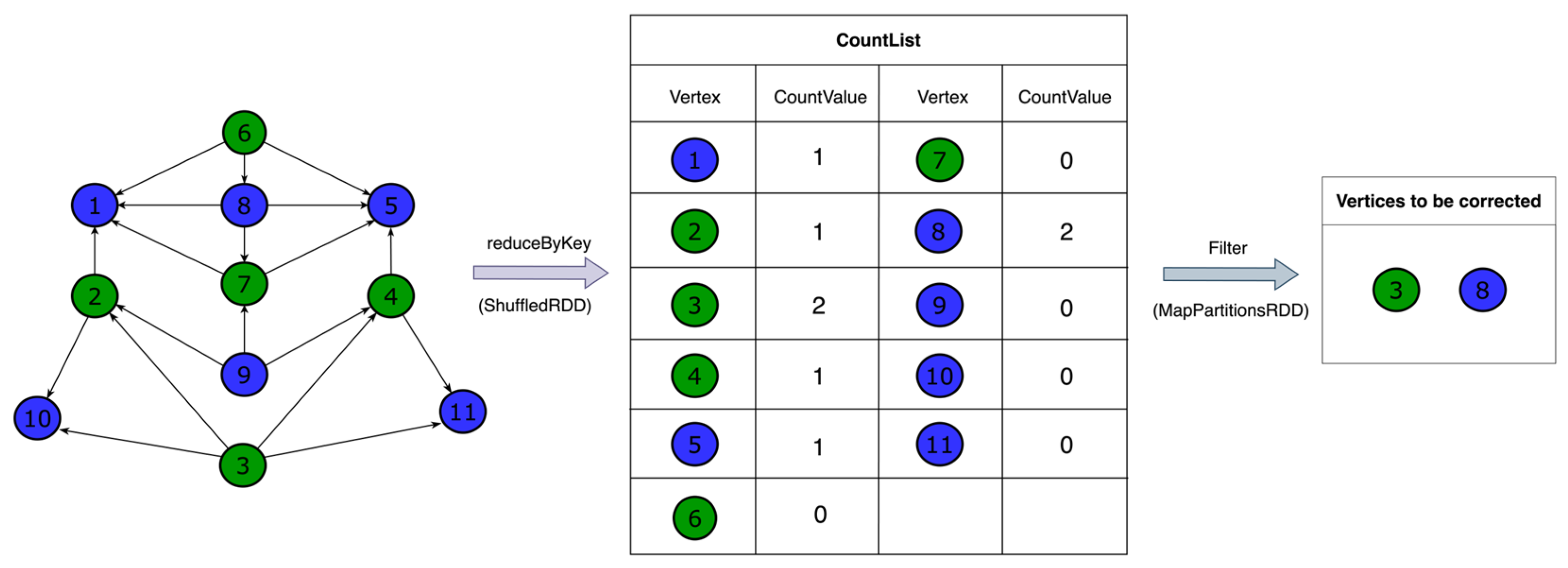
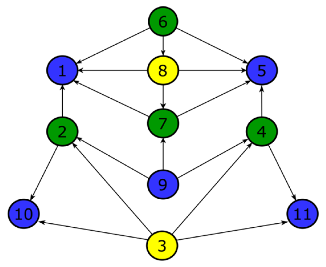
3.3. Illustrated Example

Spardex is applied to the graph in Figure 1a through four stages.

Initialization stage: The graph data is loaded from HDFS into a GraphX object and partitioned using the EdgePartition1D strategy, which distributes vertices and edges based on source vertices.

Pre-coloring stage: Each vertex broadcasts its $Id$ and degree to neighbors. The order, $j$, of each vertex is determined by degree ranking, with ties resolved by $Id$, where larger $Id$s receive smaller orders. In this case, vertex 8 has order 1; vertices 2, 3, 4, and 7 have order 2; vertices 5, 10, and 11 have order 3; and vertices 1, 6, and 9 have order 4. This order serves as the initial color, with blue (color 1) being assigned the highest priority, followed by green (color 2), yellow (color 3), and red (color 4) in descending order. The visual outputs for ComputeOrder and InitialColor are illustrated in Figure 6. The example graph is partitioned using the EdgePartition1D strategy into seven subgraphs, as shown in Figure 7.

Partitioned repaint stage: Each partition identifies the smallest $k$ unused colors and stores them in $UnusedColors$. If available, the largest-colored vertices ($MaxColor$) are reassigned to the smallest available color, with the remaining $k-1$ colors assigned accordingly. For example, in Partition 1, vertices 6 and 1 are repainted from red (color 4) to green (color 2). This process is repeated for all partitions, as shown in Figure 7. Since a vertex may receive different colors across partitions, a minor-color-first strategy ensures that each vertex retains the smallest assigned color. As illustrated in Figure 8, the entire graph is reduced to two colors (blue and green), compared with the four colors required by DistG.

Conflict Detection and Correction Stage: We can identify vertices sharing the same color with neighbors. A MapReduce-based conflict detection program locates conflicting vertices in parallel, as shown in Figure 5. The results show that vertices 8 and 3 require correction. Each is reassigned to the smallest available color, avoiding conflicts in neighbor vertices—yellow (color 3). The final graph, shown in Figure 8, demonstrates that Spardex achieves optimal coloring with only three colors, while DistG requires four, confirming its efficiency in reducing the chromatic number through parallel processing.

4. Optimization Technique

In this section, we systematically present the optimization techniques to improve the algorithm’s efficiency. We state the motivation, implementation details, and experimental comparisons between the baseline (without optimization) and the tuned version.

4.1. Data Locality Optimization in Spardex

Effective data locality optimization in Spardex requires strategic tuning of Spark’s locality wait parameters to minimize data transfer costs. The EdgePartition1D strategy inherently generates numerous small partitions [31,32], increasing network overhead if tasks are not co-located with the data. Spark defines four locality levels (PROCESS_LOCAL, NODE_LOCAL, RACK_LOCAL, ANY), prioritizing task scheduling based on data proximity [14]. By default, Spark delays task execution at each locality level before degrading to lower levels. Adjusting locality wait times ensures tasks execute closer to the data, reducing latency. Following Geng et al.’s recommendations [33], Spardex configures:

spark.locality.wait = 3 s, spark.locality.wait.node = 3 s, spark.locality.wait.rack = 3 s: Allow 3 s waits for node/rack-level locality;

spark.locality.wait.process = 1 s: Prioritizes PROCESS_LOCAL tasks with shorter wait times.

4.2. Memory Management in Spardex

Efficient memory management is crucial for preventing out-of-memory errors and optimizing Spark jobs. A key strategy involves tuning spark.memory.fraction to balance execution and storage memory, enhancing efficiency in memory-intensive tasks [33,34]. Caching frequently accessed RDDs and DataFrames can reduce computation time but must be carefully managed to prevent memory overload [34,35]. Using the MEMORY_AND_DISK storage level helps mitigate overflow while maintaining in-memory processing benefits [34]. Broadcasting large datasets minimizes memory usage by preventing redundant serialization across executors [35,36,37]. Additionally, configuring garbage collection (GC) settings, such as selecting G1GC and adjusting heap size, spark.executor.memory, and spark.executor.extraJavaOptions, can significantly improve Spark performance by reducing memory overhead [38].

Accordingly, several settings are implemented in Spardex: (1) Tune the memory fraction to ensure a balance between storage and execution memory. For Spardex, set the following parameters: (i) spark.memory.fraction = 0.6 allocates 60% of the heap space for execution and storage; (ii) spark.memory.storageFraction = 0.3 ensures 30% of the memory is reserved for caching data. (2) Cache frequently accessed RDDs or DataFrames to help reducing recomputation. (3) Use broadcast variables for distributing large read-only data across the cluster to minimize memory usage. (4) Garbage collection (GC) settings: Proper GC settings can reduce memory overhead. Use the configuration spark.executor.extraJavaOptions = −XX:+UseG1GC, which uses the G1GC garbage collector.

To quantify the impact of these settings, we applied Spardex to different optimization strategies. As shown in Figure 9, the unoptimized algorithm exhibits the highest execution time (up to 39 s in web-Google—the largest graph has 5,105,039 edges) and the lowest memory footprints (around 2.2 GB–16.1 GB) among all datasets. Introducing data-locality and memory-management tweaks shifts all points upward, reducing execution times by roughly 9–34% while slightly increasing average RAM to 4.3 GB–19.4 GB, owing to the higher spark.memory.fraction. These results demonstrate that carefully balancing execution and storage memory, combined with controlled persistence and GC tuning, materially improves both throughput and resource efficiency without altering Spardex’s core algorithmic flow.

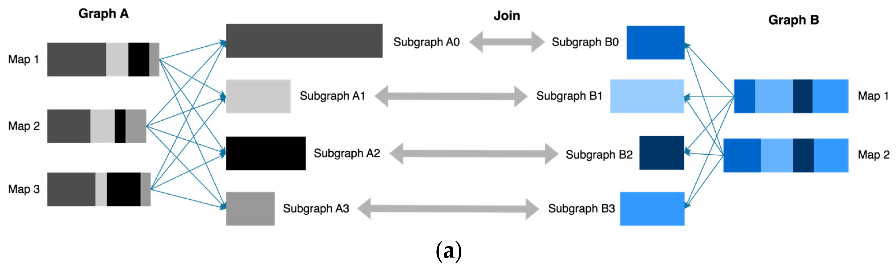
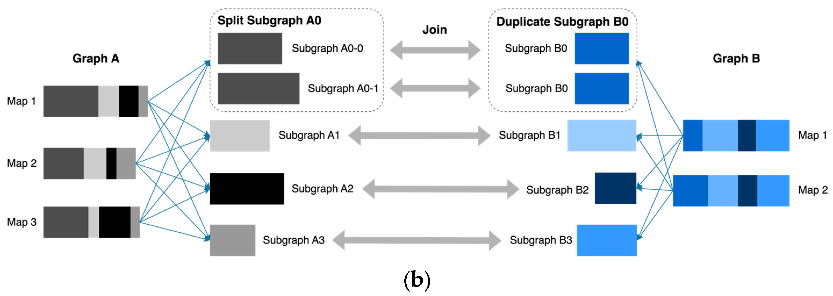
4.3. Dynamical Optimization for the Data Skew Caused by Join in Spardex

Data skew arises when partitions are unevenly distributed, leading to performance degradation during join operations. Yang et al. [39] showed that this imbalance causes certain executors to handle excessive data, resulting in idle resources and inefficient query processing. Adaptive Query Execution (AQE) mitigates this by detecting skewed partitions via shuffle file statistics and splitting them into smaller sub-partitions, ensuring a more balanced workload [40,41].

For instance, when Graph A joins Graph B (Figure 10a), Subgraph A0 is significantly larger, causing execution bottlenecks as other executors remain idle. AQE’s skew join optimization splits Subgraph A0 into smaller subgraphs, which then join their corresponding subgraphs in Graph B (Figure 10b), thus improving load balancing. Perez et al. [37] and Xu et al. [41] emphasized the importance of dynamic partitioning to prevent such bottlenecks. In our implementation, AQE is activated by setting spark.sql.adaptive.enabled = true and spark.sql.adaptive.skewJoin.enabled = true, with spark.sql.adaptive.skewJoin.skewedPartitionThresholdInBytes set to 64 MB. During execution, if a shuffle partition exceeds this size, Spark dynamically splits it into smaller units, allowing each to be joined independently and redistributed across executors to improve workload balance [39].

The experimental measurements are shown in Figure 9. Compared with the unoptimized baseline, the fully optimized algorithm achieves the best balance of speed and resource consumption: execution times decrease by 35–46%, and the average RAM per node generally settles between 3.2 GB and 18.3 GB.

5. Evaluation

In this section, we present the results of our experimental evaluation of Spardex and compare it with state-of-the-art graph coloring techniques using several frequently used graphs.

5.1. Experimental Setup

We tested our algorithm using both directed and undirected graphs. In our algorithm, undirected graphs are transformed into directed graphs in the direction from the source vertex to the destination vertex, and only one edge is preserved between the same two vertices.

We carried out the experiments on seven graphs, all obtained from the Stanford Network Analysis Project (SNAP) [42]. The maximum degree of vertices among all graphs ranged from ${10}^2$ to ${10}^5$, and the complete information for the graph datasets is shown in

Table 1. Datasets used in the experiments.

Dataset	Vertices	Edges	Max_degree	Partitions	Direction
amazon0302	262,111	1,234,877	420	257,570	Directed
Cit-HepPh	27,770	352,807	2468	25,059	Directed
com-Youtube	1,134,890	2,987,624	28,754	374,785	Undirected
email-Enron	36,692	183,831	1383	36,692	Undirected
wiki-Vote	7115	103,689	1065	6110	Directed
web-Stanford	281,903	2,312,497	38,625	281,731	Directed
web-Google	875,713	5,105,039	6332	739,454	Directed

.

We conducted the experiments using Aliyun (https://www.aliyun.com), a cloud computing service provider under the Alibaba Group providing cloud computing services such as servers, databases, and storage. To achieve our experiments, we created a Hadoop cluster with 1 master node and 10 slave nodes. Each node uses the following parameters: an Intel Core i7 processor (16 cores @ 5.2 GHz), 32 GB of RAM, running the Ubuntu 16.04.7 LTS operation system, with Hadoop version 3.2.4 and Spark version 3.2.2. We set one Spark driver and four Spark executors in each node, and the system configuration parameters selected for each Spark GraphX node are shown in

Table 2. Spark configuration parameters used in the experiments.

System Parameter	Description	Value
Spark.master	The cluster manager to connect to: “yarn” indicates that Spark runs on the Hadoop YARN resource scheduler.	yarn
Spark.executor.cores	The number of cores used on each executor to run tasks.	3
Spark.driver.cores	Number of cores used for the driver process.	3
Spark.executor.memory	Total amount of memory used per executor process.	7 g
Spark.driver.memory	Amount of memory used for the driver process.	2 g
Spark.dynamicAllocation.enabled	Whether Spark automatically adjusts the number of executors and the number of resources allocated to each executor based on the workload of the application.	true
Spark.shuffle.service.enabled	Whether the external shuffle service is set as a standalone component that manages shuffle data (intermediate data exchanged between tasks) for each node in a Spark cluster	true
Spark.serializer	“Spark.serializer” specifies the serialization mechanism Spark uses when transmitting data over the network or when storing it in memory.	org.apache.spark.serializer.KryoSerializer

.

These settings fully leverage cluster resources to jointly enhance the performance, resource utilization, and stability of Spark GraphX computations using the Hadoop cluster, thereby improving the efficiency of processing large-scale graph data.

5.2. The Algorithms for Comparison

We compared Spardex with three state-of-the-art methods: LLDF, LSLDF, and DistG.

Local Largest Degree First (LLDF) [6]: This algorithm colors vertices with the highest degrees first to reduce conflicts and potentially lower the chromatic number. While effective at minimizing conflicts, LLDF may not always yield the optimal chromatic number, particularly in irregular graphs, due to its greedy approach.

Local Smallest Largest Degree First (LSLDF) [6]: An enhancement over LLDF, LSLDF colors both the highest- and lowest-degree vertices simultaneously. This approach improves execution time and reduces the chromatic number more effectively than LLDF. However, like LLDF, it may still not achieve the optimal solution in dense graphs.

DistG [7]: A distributed graph coloring algorithm executed within the Hadoop Giraph framework. It consists of three stages: initialization, initial coloration, and conflict correction. DistG ensures efficient parallel processing, reducing execution time by minimizing supersteps and message complexity. While scalable and efficient, it may suffer from suboptimal pre-coloring and the underutilization of Pregel-like parallelism.

5.3. Experimental Results and Discussion

We evaluated the Spardex algorithm against LLDF, LSLDF, and DistG using various datasets, comparing them based on the chromatic number, execution time, and program parallelism. The comparisons were conducted under the same experimental conditions stated in Section 5.1 and Table 2.

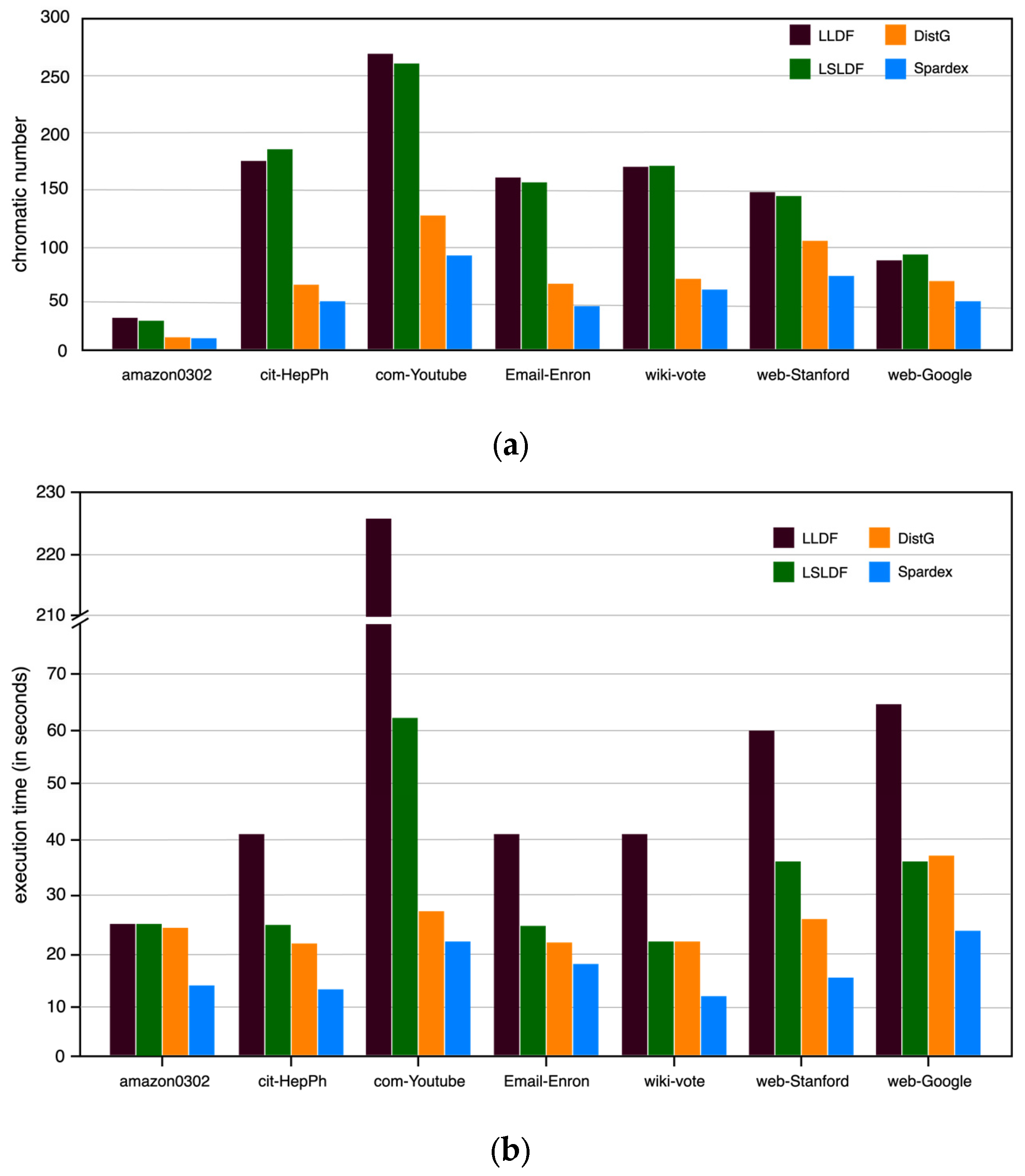
5.3.1. Performance Comparison

The comparison was based on two metrics: the number of colors used and execution time. We define the speedup of the proposed algorithm compared with the baseline algorithm as follows: $Speedup={\displaystyle \frac{T_b-T_p}{T_b}}$, where $T_b$ represents the execution time of the baseline algorithm, and $T_p$ represents the execution time of the proposed algorithm.

Table 3. Experimental results for different coloring algorithms.

Algorithm		amazon0302	cit-HepPh	com-Youtube	email-Enron	wiki-Vote	web-Stanford	web-Google	Speedup/Decrease
Spardex	time(s)	14	13	22	18	12	16	24	\
	colors	11	51	88	49	64	77	54
LLDF [6]	time(s)	26	41	226	41	41	60	65	1.86–10.27
	colors	32	177	267	160	172	149	84	36–71%
LSLDF [6]	time(s)	26	25	62	25	22	36	36	1.39–2.82
	colors	29	183	262	157	173	145	87	38–72%
DistG [7]	time(s)	25	22	27	22	22	26	27	1.13–1.83
	colors	12	65	128	69	74	104	74	8–31%

presents the experimental results, showing that Spardex achieves speedups of up to 10.27, 2.82, and 1.83 times over LLDF, LSLDF, and DistG, respectively. Spardex consistently outperforms all competitors in the chromatic number, achieving reductions of up to 71%, 72%, and 31% compared with the other three algorithms. These results are further illustrated in Figure 11a,b.

The control algorithms pre-color the graphs’ vertices and resolve conflicts in subsequent stages, aiming to minimize conflicts but not considering local optimal solutions for color reduction, as discussed in Section 3.1. For example, DistG initially assigns 81 colors to the wiki-Vote dataset’s vertices and reduces them to 74 in the conflict correction stage.

Spardex, by contrast, explicitly leverages local symmetry within each partition to drive color reduction toward locally optimal solutions rather than focusing on minimizing global conflicts. In addition, it accommodates the topological asymmetry that emerges when the graph is partitioned into subgraphs. While this strategy may increase the total partitions, the optimization techniques outlined in Section 4 allow Spardex to perform with less execution time and fewer colors than competing methods.

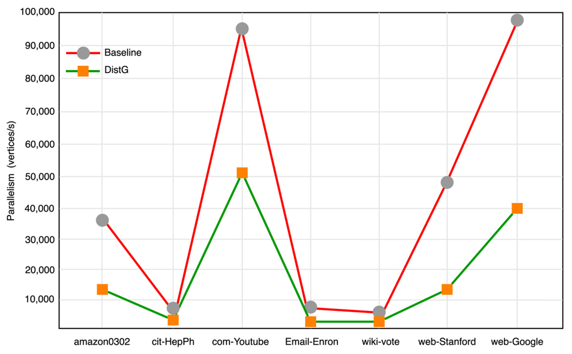
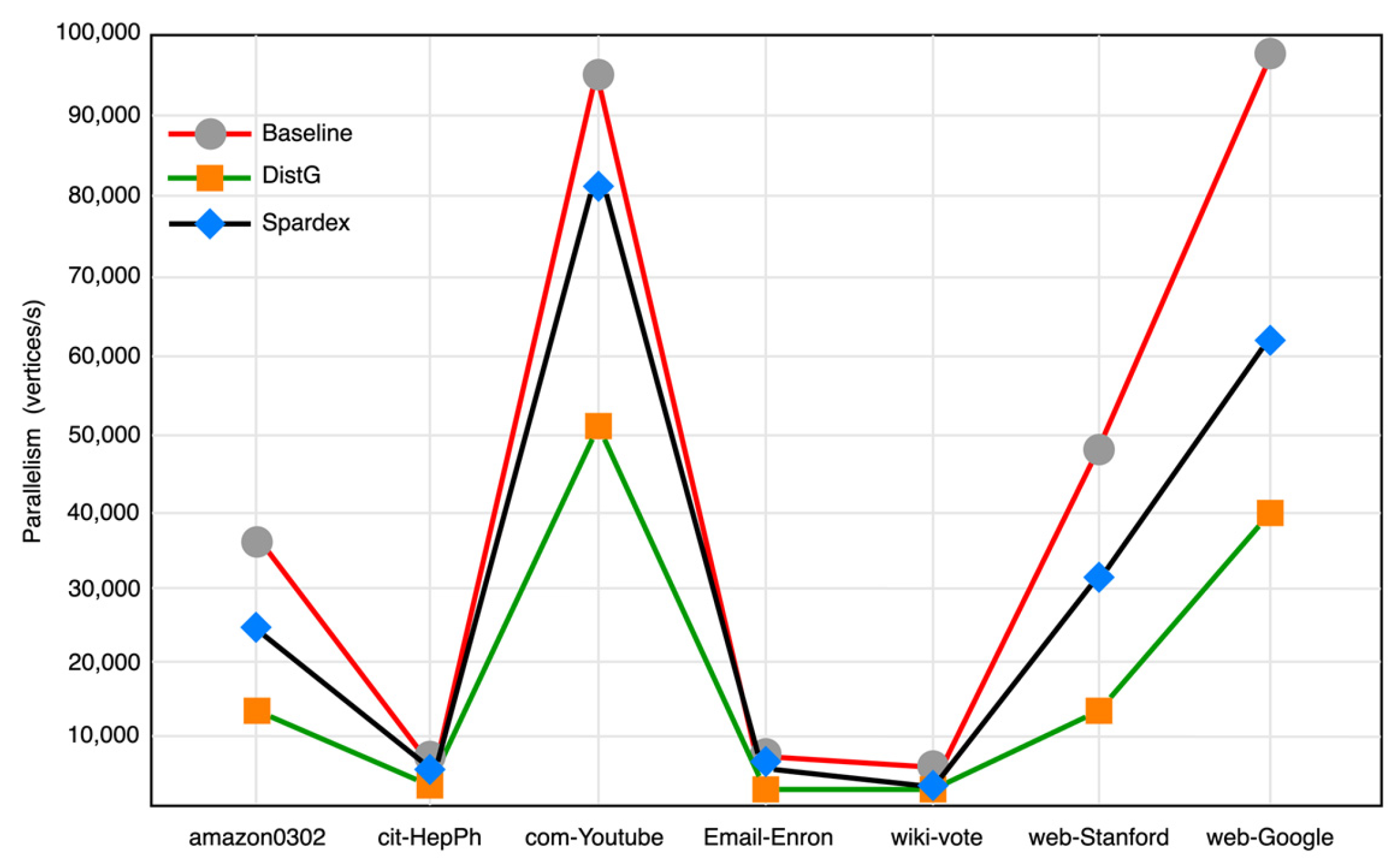
5.3.2. Parallelism Evaluation

We evaluated the parallelism of Spardex during the conflict correction stage using the same method described in Section 2: $P= {\displaystyle \frac{v.num}{T_c}}$. We conducted comparative experiments on Spardex and DistG with the baseline in the same hardware environment and Hadoop cluster. The resulting experimental data is illustrated in Figure 12.

The experimental results indicate that while Spardex still exhibits a gap compared with the baseline in the conflict correction stage, it shows significant improvement compared with the DistG algorithm [7]. This is due to the robust Spark GraphX distributed graph computing framework utilized by Spardex, along with our newly developed partitioned repaint stage and MapReduce-based conflict detection and correction algorithm.

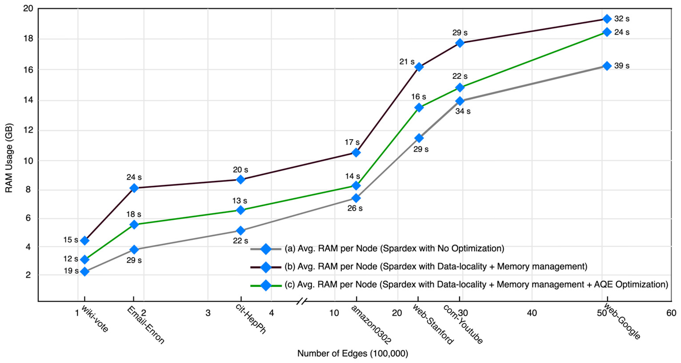
5.3.3. Complexity Analysis and Resource Usage

The performance of the Spardex algorithm is governed primarily by repeated passes over the edge set and the cost of distributed aggregation. Computing vertex degrees and propagating neighbor-degree messages with two calls to aggregateMessages, detecting conflicts, and gathering neighbor colors requires traversals of all $\left|E\right|$ edges. In addition, the conflict resolution shuffle introduces a worst-case sorting cost of $O(\left|E\right| \mathrm{l}\mathrm{o}\mathrm{g}|V\left|\right)$ during key-based grouping, where $\left|V\right|$ denotes the number of vertices. As a result, the end-to-end time complexity of a single Spardex iteration can be expressed as $O(\left|E\right| \mathrm{l}\mathrm{o}\mathrm{g}\left|V\right| +|V\left|\right)$, where, for most practical graphs, $\left|E\right|\gg \left|V\right|$ behaves nearly linearly in the number of edges. Thus, the time complexity of Spardex can be simplified as $O(\left|E\right| \mathrm{l}\mathrm{o}\mathrm{g}|V\left|\right)$.

Memory requirements arise from storing both the original GraphX edge RDD and the various vertex RDDs (degrees, colors, and conflict detections) together with intermediate message buffers used during shuffle operations. Since each edge may emit, at most, a constant number of messages, and each vertex maintains a small color or degree record, the total resident data scales as $O(\left|E\right|+|V\left|\right)$.

Figure 9 presents measurements of the average RAM per node and execution time under three different optimization settings: (a) Spardex with no optimizations, (b) Spardex with data locality and memory management tuning, and (c) Spardex with data locality, memory management, and AQE optimization. Each point in the scatter plot denotes one of the experiment results conducted using the same seven test graphs listed in Table 1. The horizontal axis reports the number of edges in different graphs, the vertical axis reports average per-node RAM usage, and the $k \mathrm{s}$ numbers beside each point show the total execution time. The Spardex algorithm is fully optimized by the optimization strategies introduced in Section 4 and achieves the best balance of speed and resource consumption: execution times decrease by an additional 17–35% relative to the two-stage tuning, and average RAM per node falls by 5–17%.

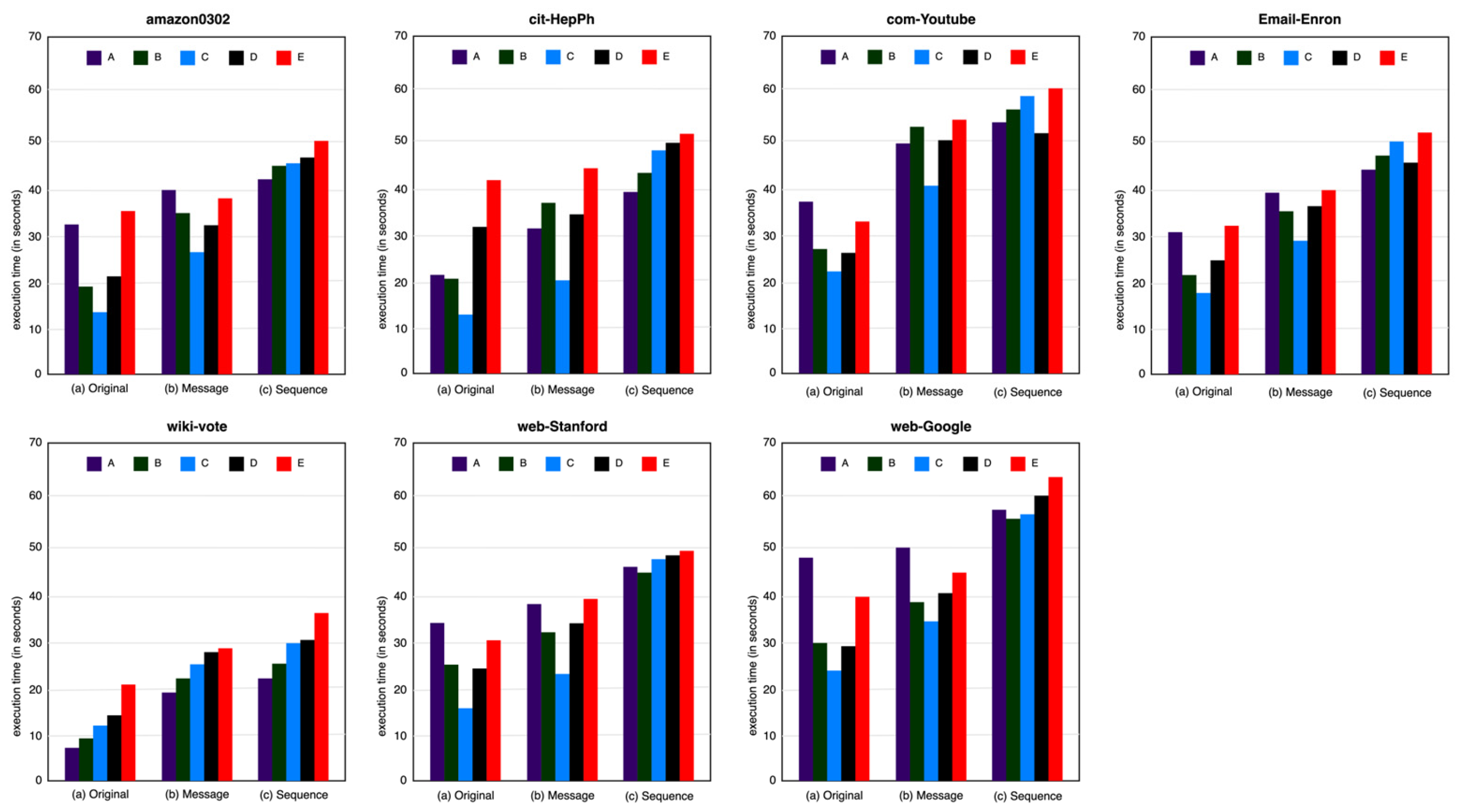
5.4. Running Spardex on Different Cluster Configurations

To demonstrate the performance of Spardex with different cluster configurations, we compare five system configuration parameters listed in

Table 4. Different system configuration parameters for comparison.

	System Parameter	Spark.executor.cores	Spark.executor.memory	Spark.driver.cores	Spark.driver.memory	Executors in Each Node
Configuration Types
A		6	14 GB	3	2 GB	2
B		4	9 GB	3	2 GB	3
C		3	7 GB	3	2 GB	4
D		2	4.5 GB	3	2 GB	6
E		1	2.5 GB	3	2 GB	12

within the same hardware environment as that introduced in Section 5.1.

In Spardex, tasks are evenly distributed among executors, with larger, more complex datasets benefiting from its high parallelism. Figure 13 shows that configuration C achieves the shortest execution time across most datasets under the original Spardex algorithm. The wiki-vote dataset, with fewer vertices and partitions, demonstrates less distribution due to fewer executors per node. Overall, configuration C provides the highest execution efficiency.

We also carried out experiments under Message-version Spardex and Sequence-version Spardex. Message-version Spardex is the pruned Spardex algorithm after removing the conflict detection and correction stage; thus, conflict correction completely depends on the message communication between vertices. As shown in Figure 13, configuration C still achieves the best execution performance across most graphs. Sequence-version Spardex is the pruned Spardex algorithm after removing the partitioned repaint stage and conflict detection and correction stage, which means conflict correction depends entirely on vertex-by-vertex sequential correction. In this case, configuration A performs better than the other configurations because fewer executors create fewer communication costs in sequential execution.

The results indicate that as the complexity and size of the dataset increase, the efficiency gains from high parallelism become more pronounced. This suggests that the Spardex algorithm is particularly well suited for large-scale graph processing tasks.

6. Conclusions and Future Opportunities

In this study, we presented Spardex, a highly efficient parallel and distributed graph coloring algorithm based on Spark GraphX. Spardex leverages the power of distributed computing to manage and color large-scale graphs effectively, significantly enhancing overall performance. Combining partitioned graph repaint with MapReduce-based conflict detection and correction, Spardex maximizes parallelism and minimizes execution time, achieving chromatic number reduction of up to 72% and a time speedup of up to 10.27 times over the previous methods.

Extensive experiments demonstrated the high effectiveness of Spardex, particularly in configurations optimized for execution efficiency. The algorithm’s adaptability to larger and more complex datasets further underscores its robustness. However, several limitations remain. First, Spardex targets static graphs and requires full re-computation when the graph structure changes, limiting its suitability for dynamic or streaming graphs. Second, the algorithm assumes unweighted and unlabeled graphs, reducing its applicability in scenarios where vertex or edge attributes are essential, such as priorities or capacities.

In future work, we will explore additional aspects of graph coloring, such as optimizing communication between executors [8,43], dynamically adjusting parallelism during runtime [25,44], and extending the algorithm to support other graph-processing tasks [45,46]. We also aim to test Spardex on a wider variety of datasets from different domains [17,47] in order to enhance its applicability and performance.

References

1. Jones, M.T.; Plassmann, P.E. A parallel graph coloring heuristic. SIAM J. Sci. Comput. 1993, 14, 654–669. [Google Scholar] [CrossRef]
2. Luby, M. A simple parallel algorithm for the maximal independent set problem. SIAM J. Comput. 1986, 15, 1036–1053. [Google Scholar] [CrossRef]
3. Bui, T.N.; Jones, C. Finding good approximate vertex and edge partitions is NP-hard. Inf. Process. Lett. 1993, 42, 153–159. [Google Scholar] [CrossRef]
4. Berman, P.; Karpinski, M. On some tighter inapproximability results. In Proceedings of the Twenty-Sixth Annual ACM Symposium on Theory of Computing, Prague, Czech Republic, 11–15 July 1999; Springer: Berlin/Heidelberg, Germany, 1999; pp. 301–309. [Google Scholar]
5. Naumov, M.; Castonguay, P.; Cohen, J. Parallel Graph Coloring with Applications to the Incomplete-LU Factorization on the GPU; Nvidia White Paper; May 2015. Available online: https://research.nvidia.com/sites/default/files/pubs/2015-05_Parallel-Graph-Coloring/nvr-2015-001.pdf (accessed on 26 May 2024).
6. Misra, J.; Gries, D. A constructive proof of Vizing’s theorem. Inf. Process. Lett. 1992, 41, 131–133. [Google Scholar] [CrossRef]
7. Brighen, A.; Slimani, H.; Rezgui, A.; Kheddouci, H. A new distributed graph coloring algorithm for large graphs. Clust. Comput. 2024, 27, 875–891. [Google Scholar] [CrossRef]
8. Schuetz, M.J.A.; Brubaker, J.K.; Zhu, Z.; Katzgraber, H.G. Graph coloring with physics-inspired graph neural networks. Phys. Rev. Res. 2022, 4, 043131. [Google Scholar] [CrossRef]
9. Grosset, A.V.P.; Zhuand, P.; Venkatasubramanian, S.; Hall, M. Evaluating graph coloring on GPUs. In Proceedings of the PPoPP’11 Proceedings of the 16th ACM Symposium on Principles and Practice of Parallel Programming, San Antonio, TX, USA, 12–16 February 2011; ACM SIGPLAN Notices-PPoPP’11. Volume 46, pp. 297–298. [Google Scholar] [CrossRef]
10. Zheng, Z.; Shi, X.; He, L.; Jin, H.; Wei, S.; Dai, H.; Peng, X. Feluca: A two-stage graph coloring algorithm with color-centric paradigm on GPU. IEEE Trans. Parallel Distrib. Syst. 2020, 32, 160–173. [Google Scholar] [CrossRef]
11. Che, S.; Rodgers, G.; Beckmann, B.; Reinhardt, S. Graph coloring on the GPU and some techniques to improve load imbalance. In Proceedings of the 2015 IEEE International Parallel and Distributed Processing Symposium Workshop, Hyderabad, India, 25–29 May 2015; pp. 610–617. [Google Scholar]
12. Boman, E.G.; Devine, K.D.; Rajamanickam, S. Scalable matrix computations on large scale-free graphs using 2D graph partitioning. In Proceedings of the International Conference for High Performance Computing, Networking, Storage and Analysis, Denver, CO, USA, 17–22 November 2013; pp. 1–12. [Google Scholar] [CrossRef]
13. Gandhi, N.M.; Misra, R. Performance comparison of parallel graph coloring algorithms on bsp model using hadoop. In Proceedings of the 2015 International Conference on Computing, Networking and Communications (ICNC), Garden Grove, CA, USA, 25–29 May 2015; pp. 110–116. [Google Scholar] [CrossRef]
14. Sharafeldeen, A.; Alrahmawy, M.; Elmougy, S. Graph partitioning MapReduce-based algorithms for counting triangles in large-scale graphs. Sci. Rep. 2023, 13, 166. [Google Scholar] [CrossRef]
15. Leighton, F.T. Introduction to Parallel Algorithms and Architectures: Arrays, Trees, Hypercubes; Elsevier: Amsterdam, The Netherlands, 1985. [Google Scholar]
16. Gebremedhin, A.H.; Manne, F.; Pothen, A. What color is your Jacobian? Graph coloring for computing derivatives. SIAM Rev. 2002, 44, 347–355. [Google Scholar] [CrossRef]
17. Alon, N.; Kahale, N. A spectral technique for coloring random 3-colorable graphs. SIAM J. Comput. 1997, 26, 1733–1748. [Google Scholar] [CrossRef]
18. Gavril, F. Algorithms for a maximum clique and a maximum independent set of a circle graph. Networks 1972, 2, 211–221. [Google Scholar] [CrossRef]
19. Galinier, P.; Hao, J.K. Hybrid Evolutionary Algorithms for Graph Coloring. J. Comb. Optim. 1999, 3, 379–397. [Google Scholar] [CrossRef]
20. Eiben, A.E.; Van Der Hauw, J.K.; van Hemert, J.I. Graph coloring with adaptive evolutionary algorithms. J. Heuristics 1998, 4, 25–46. [Google Scholar] [CrossRef]
21. Vizing, V.G. On an estimate of the chromatic class of a p-graph. Diskret. Analiz 1964, 3, 25–30. [Google Scholar]
22. Chung, F.R.K.; Lu, L. The average distances in random graphs with given expected degrees. Proc. Natl. Acad. Sci. USA 2002, 99, 15879–15882. [Google Scholar] [CrossRef]
23. Edmonds, J. Paths, Trees, and Flowers. Can. J. Math. 1965, 17, 449–467. [Google Scholar] [CrossRef]
24. Karypis, G.; Kumar, V. A fast and high quality multilevel scheme for partitioning irregular graphs. SIAM J. Sci. Comput. 1998, 20, 359–392. [Google Scholar] [CrossRef]
25. Gibbons, P.B. A more practical PRAM model. In Proceedings of the First Annual ACM Symposium on Parallel Algorithms and Architectures, Santa Fe, NM, USA, 18–21 June 1989; pp. 158–168. [Google Scholar]
26. Kawarabayashi, K.; Khoury, S.; Schild, A.; Schwartzman, G. Improved distributed approximations for maximum independent set. arXiv 2019, arXiv:1906.11524. [Google Scholar] [CrossRef]
27. Tarjan, R.E. Depth-first search and linear graph algorithms. SIAM J. Comput. 1972, 1, 146–160. [Google Scholar] [CrossRef]
28. Hopcroft, J.E.; Tarjan, R.E. Algorithm 447: Efficient algorithms for graph manipulation. Commun. ACM 1973, 16, 372–378. [Google Scholar] [CrossRef]
29. Karger, D.R.; Stein, C. A new approach to the minimum cut problem. J. ACM 1996, 43, 601–640. [Google Scholar] [CrossRef]
30. Tarjan, R.E. Efficiency of a good but not linear set union algorithm. J. ACM 1975, 22, 215–225. [Google Scholar] [CrossRef]
31. Geng, Y.; Shi, X.; Pei, C.; Jin, H.; Jiang, W. LCS: An Efficient Data Eviction Strategy for Spark. Int. J. Parallel Prog. 2017, 45, 1285–1297. [Google Scholar] [CrossRef]
32. Yao, Y. A Partition Model of Granular Computing. In Transactions on Rough Sets I. Lecture Notes in Computer Science; Peters, J.F., Skowron, A., Grzymała-Busse, J.W., Kostek, B., Świniarski, R.W., Szczuka, M.S., Eds.; Springer: Berlin/Heidelberg, Germany, 2004; Volume 3100. [Google Scholar] [CrossRef]
33. Adinew, D.M.; Zhou, S.; Liao, Y. Spark performance optimization analysis in memory management with deploy mode in standalone cluster computing. In Proceedings of the 2020 IEEE 36th International Conference on Data Engineering (ICDE), Dallas, TX, USA, 20–24 April 2020; pp. 2049–2053. [Google Scholar] [CrossRef]
34. Wang, S.; Zhang, Y.; Zhang, L.; Cao, N.; Pang, C. An Improved Memory Cache Management Study Based on Spark. Comput. Mater. Contin. 2018, 56, 415–431. [Google Scholar]
35. Gannon, D.; Jalby, W.; Gallivan, K. Strategies for cache and local memory management by global program transformation. In International Conference on Supercomputing; Springer: Berlin/Heidelberg, Germany, 1987; pp. 229–254. [Google Scholar]
36. Tang, Z.; Zeng, A.; Zhang, X.; Yang, L.; Li, K. Dynamic memory-aware scheduling in spark computing environment. J. Parallel Distrib. Comput. 2020, 141, 10–22. [Google Scholar] [CrossRef]
37. Perez, T.B.; Zhou, X.; Cheng, D. Reference-distance eviction and prefetching for cache management in spark. In Proceedings of the 47th International Conference on Parallel Processing, Eugene, OR, USA, 13–16 August 2018; pp. 1–10. [Google Scholar] [CrossRef]
38. Zhou, P.; Ruan, Z.; Fang, Z.; Shand, M.; Roazen, D.; Cong, J. Doppio: I/o-aware performance analysis, modeling and optimization for in-memory computing framework. In Proceedings of the 2018 IEEE International Symposium on Performance Analysis of Systems and Software (ISPASS), Belfast, UK, 2–4 April 2018; pp. 22–32. [Google Scholar] [CrossRef]
39. Yang, Z.; Jia, D.; Ioannidis, S.; Mi, N.; Sheng, B. Intermediate data caching optimization for multi-stage and parallel big data frameworks. In Proceedings of the 2018 IEEE 11th International Conference on Cloud Computing (CLOUD), San Francisco, CA, USA, 2–7 July 2018; pp. 277–284. [Google Scholar] [CrossRef]
40. Huang, S.; Huang, J.; Dai, J.; Xie, T.; Huang, B. The HiBench benchmark suite: Characterization of the MapReduce-based data analysis. In Proceedings of the 2010 IEEE 26th International Conference on Data Engineering Workshops (ICDEW 2010), Long Beach, CA, USA, 1–6 March 2010; pp. 41–51. [Google Scholar] [CrossRef]
41. Bhattacharjee, A. Large-reach memory management unit caches. In Proceedings of the 46th Annual IEEE/ACM International Symposium on Microarchitecture (MICRO-46), Davis, CA, USA, 7–11 December 2013; Association for Computing Machinery: New York, NY, USA, 2013; pp. 383–394. [Google Scholar] [CrossRef]
42. Leskovec, J.; Krevl, A. Snap Datasets: Stanford Large Network Dataset Collection. 2014. Available online: http://snap.stanford.edu/data (accessed on 26 May 2024).
43. Blelloch, G.E.; Maggs, B.M. Parallel algorithms. Commun. ACM 1996, 39, 85–97. [Google Scholar] [CrossRef]
44. Alon, N.; Spencer, J.H. The Probabilistic Method; John Wiley & Sons: Hoboken, NJ, USA, 2016. [Google Scholar]
45. Papadimitriou, C.H. Computational complexity. In Encyclopedia of Computer Science; John Wiley and Sons Ltd.: Hoboken, NJ, USA, 2003; pp. 260–265. [Google Scholar]
46. Matula, D.W.; Beck, L.L. Smallest-last ordering and clustering and graph coloring algorithms. J. ACM 1983, 30, 417–427. [Google Scholar] [CrossRef]
47. Arora, S.; Safra, S. Probabilistic checking of proofs: A new characterization of NP. J. ACM 1998, 45, 70–122. [Google Scholar] [CrossRef]
Figure 2. A possible better solution using the graph in Figure 1a.
Symmetry 17 01177 g002
Figure 3. Comparison of parallelism between DistG and the baseline in the conflict correction stage.
Symmetry 17 01177 g003
Figure 4. Flowchart of Spardex algorithm.
Symmetry 17 01177 g004
Figure 6. Visual pipeline of the ComputeOrder and InitialColor operating on Figure 1a. The “ k d ” labels beside the vertices in the uncolored graph are the degrees of each vertex.
Symmetry 17 01177 g006
Figure 7. The partitioned repaint stage in Spardex. “ M a x C o l o r ” and “ U n u s e d C o l o r s ” are the maximum used colors in each partition and the unused color set for each partition used to decide the vertices to be repainted.
Symmetry 17 01177 g007
Figure 8. The conflict detection and correction stage in Spardex. Vertex 3 has two neighbor colors (blue and green), and the minimum available color is yellow (color 3), like vertex 8. Thus, vertices 3 and 8 are both corrected with yellow. The final corrected graph contains only three colors.
Symmetry 17 01177 g008
Figure 9. Average RAM per node and total execution time using (a) Spardex with no optimization; (b) Spardex with data locality and memory management; and (c) Spardex with data locality, memory management, and AQE optimization.
Symmetry 17 01177 g009
Figure 10. Schematic of AQE skew join optimization. (a) Illustration of subgraph merging without AQE skew join optimization enabled; (b) illustration of subgraph merging with AQE skew join optimization enabled.
Symmetry 17 01177 g010aSymmetry 17 01177 g010b
Figure 11. Performance comparison between Spardex and three competitive algorithms in terms of (a) chromatic number and (b) execution time.
Symmetry 17 01177 g011
Figure 12. Comparison of parallelism between DistG, Spardex, and the baseline in the conflict correction stage.
Symmetry 17 01177 g012
Figure 13. Execution time resulting from different system configuration parameters under three pruned version algorithms. (a) Original: The Spardex algorithm proposed in this study. (b) Message: The pruned Spardex algorithm after removing the conflict detection and correction stage. (c) Sequence: The pruned Spardex algorithm after removing the partitioned repaint stage and conflict detection and correction stage.
Symmetry 17 01177 g013