Gregory Polynomials Within Sakaguchi-Type Function Classes: Analytical Estimates and Geometric Behavior

Abstract

This work introduces a novel family of analytic and univalent functions formulated through the integration of Gregory coefficients and Sakaguchi-type functions. Employing subordination techniques, we obtain sharp bounds for the initial coefficients in their Taylor expansions. The influence of parameter variations is examined through comprehensive geometric visualizations, which confirm the non-emptiness of the class and provide insights into its structural properties. Furthermore, Fekete–Szegö inequalities are established, enriching the theory of bi-univalent functions. The combination of analytical methods and geometric representations offers a versatile framework for future research in geometric function theory.

1. Introduction, Definitions and Motivation

The study of special sequences, such as the Fibonacci, Pell, and Lucas numbers, has long been a cornerstone of Geometric Function Theory. These sequences provide essential tools for defining and analyzing subclasses of analytic and univalent functions. In recent years, considerable attention has been devoted to exploring the coefficients arising in the Taylor–Maclaurin expansions of analytic functions defined on the open unit disk, motivated by classical results from the Riemann mapping theorem and the foundational contributions of Koebe and Bieberbach.

Among these special sequences, the Gregory coefficients—first introduced by James Gregory in 1670—stand out due to their appearance in numerical integration, interpolation formulas, and series expansions. They have been rediscovered in various contexts by prominent mathematicians such as Laplace, Mascheroni, Fontana, Bessel, Clausen, Hermite, Pearson, and Fisher. As a result, they are known by various names in the literature, including reciprocal logarithmic numbers, Bernoulli numbers of the second kind, normalized generalized Bernoulli numbers, and normalized Cauchy numbers of the first kind.

We start this section by defining the Gregory coefficients, which will be used in constructing our new class of analytic functions.

Gregory coefficients naturally arise in diverse areas of mathematics, particularly in numerical analysis, approximation theory, and number theory. They serve as rational constants in the Maclaurin series expansion of the reciprocal logarithm and are given by:

$${\displaystyle \frac{1}{2}},-{\displaystyle \frac{1}{12}},{\displaystyle \frac{1}{24}},-{\displaystyle \frac{19}{720}},{\displaystyle \frac{3}{160}},-{\displaystyle \frac{863}{60480}},\dots$$

To better understand the structure, we consider their generating function (see [1,2,3,4,5,6]):

$$\begin{array}{cc}\hfill \mathfrak{G}\left(z\right)& ={\displaystyle \frac{z}{log(1+z)}}\hfill \\ \hfill & =\sum _{n=0}^{\infty }{\Lambda }_n{z}^n\hfill \\ \hfill & =1+{\displaystyle \frac{1}{2}}z-{\displaystyle \frac{1}{12}}{z}^2+{\displaystyle \frac{1}{24}}{z}^3-{\displaystyle \frac{19}{720}}{z}^4+{\displaystyle \frac{3}{160}}{z}^5+\dots ,\hfill \end{array}$$

(1)

where $z\in \mathfrak{U}=\{z\in \mathbb{C}:|z|<1\}$, and log is considered on the principal branch. The coefficients ${\Lambda }_n$ are called the Gregory coefficients, with ${\Lambda }_0=1$. They can also be defined via the recurrence relation [7,8]:

$$\begin{array}{c}\hfill {\Lambda }_n={\displaystyle \frac{{(-1)}^{n-1}}{n+1}}+\sum _{k=1}^{n-1}{\displaystyle \frac{{(-1)}^{n+1-k}{\Lambda }_k}{n+1-k}},n\ge 2,\end{array}$$

(2)

or by means of the Stirling numbers of the first kind $S_1(n,l)$:

$${\Lambda }_n={\displaystyle \frac{1}{n!}}\sum _{l=1}^n{\displaystyle \frac{S_1(n,l)}{l+1}},$$

(3)

where Stirling numbers $S_1(n,l)$ are given by:

$$S_1(n,l)=\left\{\begin{array}{ll}{\displaystyle \frac{(2n-l)!}{(l-1)!}\sum _{k=0}^{n-l}\frac{1}{(n+k)(n-l-k)!(n-l+k)!}\sum _{r=0}^k\frac{{(-1)}^r{r}^{n-l+k}}{r!(k-r)!},}& l\in [1,n],\hfill \\ 1,& n=0,l=0,\\ 0,& \mathrm{otherwise}.\end{array}\right.$$

For example, the values of $S_1(n,l)$ for small n and l are:

$$\begin{array}{ccc}{S}_1(1,1)=1,& S_1(2,1)=-1,& S_1(2,2)=1,\\ S_1(3,1)=2,& S_1(3,2)=-3,& S_1(3,3)=1.\end{array}$$

Thus, the first few Gregory coefficients are given by:

$${\Lambda }_1={\displaystyle \frac{1}{2}},{\Lambda }_2=-{\displaystyle \frac{1}{12}},{\Lambda }_3={\displaystyle \frac{1}{24}},{\Lambda }_4=-{\displaystyle \frac{19}{720}},\dots .$$

The sequence exhibits deep connections with Bernoulli numbers of the second kind and Cauchy numbers, forming a link between combinatorial structures and analytic functions. This relationship has been rigorously established in the literature, where Gregory coefficients are shown to coincide with the Cauchy numbers of the first kind and the Bernoulli numbers of the second kind. In addition to their generating function representation in (1), the recurrence relation in (2), and the Stirling-based expression in (3), the Gregory coefficients ${\Lambda }_n$ can also be written as

$${\Lambda }_n={\displaystyle \frac{C_{1,n}}{n!}}={\displaystyle \frac{B_n^{\left(n\right)}}{n!}}={\displaystyle \frac{1}{n!}}\sum _{l=1}^n{\displaystyle \frac{S_1(n,l)}{l+1}},$$

where $C_{1,n}$ are the Cauchy numbers of the first kind, $B_n^{\left(n\right)}$ denote the Bernoulli numbers of the second kind, and $S_1(n,l)$ are the Stirling numbers of the first kind. These representations illustrate how Gregory coefficients serve as a unifying structure connecting classical number sequences with both analytical and combinatorial frameworks. Such identities play a central role in summation techniques and approximation formulas, as emphasized by Merlini et al. [9] and also Blagouchine and Qi and Zhao [6,8,10], who collectively confirm the equivalence and recurrence of Gregory coefficients under various names and contexts. For further details and related developments, see also [2,11,12,13,14,15,16], and the references therein.

Now, we present the foundational definitions and concepts concerning analytic functions and related subclasses, which will be employed in the subsequent formulation and analysis of our proposed function class.

Let $\mathcal{A}$ be the set of all functions that are analytic in the open unit disk $\mathfrak{U}$ and satisfy the normalization conditions:

$$\mathfrak{F}\left(0\right)=0\mathrm{and}{\mathfrak{F}}^{\prime }\left(0\right)=1.$$

Any function $\mathfrak{F}\in \mathcal{A}$ meeting these criteria can be expressed using its Taylor–Maclaurin series as follows:

$$\mathfrak{F}\left(z\right)=z+\sum _{n=2}^{\infty }{a}_n{z}^n.$$

(4)

Consider the subclass:

$$\mathcal{S}=\left\{\mathfrak{F}\in \mathcal{A}:\mathfrak{F}\mathrm{is}\mathrm{univalent}\mathrm{in}\mathfrak{U}\right\},$$

which consists of those functions in $\mathcal{A}$ that are one-to-one (univalent) within $\mathfrak{U}$.

The Koebe One-Quarter Theorem [17] states that every function in $\mathcal{S}$ maps the open unit disk $\mathfrak{U}$ onto a region that includes a disk of radius ${\displaystyle \frac{1}{4}}$. As a consequence, any $\mathfrak{F}\in \mathcal{S}$ has an inverse function ${\mathfrak{F}}^{-1}$ that satisfies:

$${\mathfrak{F}}^{-1}\left(\mathfrak{F}\left(z\right)\right)=z\mathrm{and}\mathfrak{F}\left({\mathfrak{F}}^{-1}\left(w\right)\right)=w\mathrm{for}\left|w\right|<R_0\left(\mathfrak{F}\right),$$

where $R_0\left(\mathfrak{F}\right)\ge {\displaystyle \frac{1}{4}}.$ The inverse function

$$\mathfrak{g}\left(w\right)={\mathfrak{F}}^{-1}\left(w\right)$$

can be expressed by the following series expansion:

$$\mathfrak{g}\left(w\right)={\mathfrak{F}}^{-1}\left(w\right)=w-a_2{w}^2+\left(2a_2^2-a_3\right)w^3-\left(5a_2^3-5a_2{a}_3+a_4\right)w^4+\dots .$$

(5)

Denote by $\Sigma$ the set containing all functions that are bi-univalent within the open unit disk $\mathfrak{U}$. Several notable functions in this category, which have been extensively studied in bi-univalent function theory, include:

$${\mathfrak{F}}_1\left(z\right)={\displaystyle \frac{z}{1-z}},{\mathfrak{F}}_2\left(z\right)=log\left({\displaystyle \frac{1}{1-z}}\right),{\mathfrak{F}}_3\left(z\right)=log\sqrt{{\displaystyle \frac{1+z}{1-z}}}.$$

These functions have the following inverse representations:

$${\mathfrak{F}}_1^{-1}\left(w\right)={\displaystyle \frac{w}{1+w}},{\mathfrak{F}}_2^{-1}\left(w\right)={\displaystyle \frac{e^w-1}{e^w}},{\mathfrak{F}}_3^{-1}\left(w\right)={\displaystyle \frac{e^{2w}-1}{e^{2w}+1}}.$$

The investigation into the coefficient bounds of these functions was initially introduced by Lewin (1967) [18], who provided an estimate for the second coefficient, stating that $|a_2|<1.51$. Subsequently, this estimate was refined by Brannan and Taha [19], who established an improved bound of $|a_2|\le \sqrt{2}$. Over the years, the study of initial coefficients has garnered substantial attention, leading to an extensive body of literature. Despite these advances, the determination of general coefficient bounds, particularly for $|a_n|$ for $n\ge 4$, remains relatively under explored. Although some progress has been made, obtaining precise estimates for higher-order coefficients continues to pose a challenging open problem. The historical estimates of the initial coefficients $a_n$ for bi-univalent functions in $\Sigma$ are summarized in

Table 1. Literature summary on the coefficients $a_n$ for functions in $\Sigma$.

Researchers	Estimates
Lewin 1967 [18]	$|a_2|\le 1.51$
Brannan and Clunie 1980 [19]	$|a_2|\le \sqrt{2}$
Netanyahu 1969 [20]	${max}_{f\in \Sigma }\left|a_2\right|={\displaystyle \frac{4}{3}}.$
Tan 1984 [21]	$|a_2|\le 1.485$
Different researchers [22,23,24,25,26]	$|a_2|$ and $|a_3|$
Open Problem [27,28]	$|a_n|$ unresolved

.

Let $\mathcal{P}$ represent the class of functions that are analytic within the unit disk $\mathfrak{U}$, normalized such that $p\left(0\right)=1$, and satisfy the positivity condition:

$$\Re \left(p\left(z\right)\right)>0,z\in \mathfrak{U}.$$

with the series expansion

$$p\left(z\right)=1+p_{1}z+p_2{z}^2+\cdots ,$$

(6)

This family is widely recognized as the Carathéodory class of functions.

The concept of subordination plays a pivotal role in analyzing the geometric and analytic properties of certain subclasses of univalent functions. The foundational framework for this notion was introduced by Lindelöf [29], while further significant contributions were made through comprehensive studies by Rogosinski [30,31] and Littlewood [32].

A function w is called a Schwarz function if it is analytic in the open unit disk $\mathfrak{U}$, satisfies $w\left(0\right)=0$, and remains bounded in modulus by 1 throughout $\mathfrak{U}$; that is,

$$w\left(0\right)=0\mathrm{and}\left|w\right(z\left)\right|<1\mathrm{for}\mathrm{all}z\in \mathfrak{U}.$$

Using this notion, let $\mathfrak{F},\mathfrak{H}$ be analytic functions in $\mathfrak{U}$. We say that $\mathfrak{F}$ is subordinate to $\mathfrak{H}$ in $\mathfrak{U}$, written as

$$\mathfrak{F}\prec \mathfrak{H}\mathrm{or}\mathfrak{F}\left(z\right)\prec \mathfrak{H}\left(z\right),$$

if there exists a Schwarz function w such that

$$\mathfrak{F}\left(z\right)=\mathfrak{H}\left(w\right(z\left)\right),z\in \mathfrak{U}.$$

Notably, if $\mathfrak{H}$ is univalent in $\mathfrak{U}$, then

$$\mathfrak{F}\prec \mathfrak{H}⟺\mathfrak{F}\left(0\right)=\mathfrak{H}\left(0\right)\mathrm{and}\mathfrak{F}\left(\mathfrak{U}\right)\subset \mathfrak{H}\left(\mathfrak{U}\right).$$

The notion of quasi-subordination was first introduced by Robertson [33]: Let $\mathfrak{F}$ and $\mathfrak{H}$ be analytic in the open unit disk $\mathfrak{U}$. $\mathfrak{F}$ is said to be quasi-subordinate to the function $\mathfrak{H}$, written as

$$\mathfrak{F}\left(z\right){\prec }_q\mathfrak{H}\left(z\right)(z\in \mathfrak{U}),$$

if there exist analytic functions $\varphi$, with $\left|\varphi \right(z\left)\right|\le 1$ such that the function ${\displaystyle \frac{\mathfrak{F}\left(z\right)}{\varphi \left(z\right)}}$ is analytic in $\mathfrak{U}$ and ${\displaystyle \frac{\mathfrak{F}\left(z\right)}{\varphi \left(z\right)}}\prec \mathfrak{H}\left(z\right)$, if there exists the above-mentioned Schwarz function w such that

$$\mathfrak{F}\left(z\right)=\varphi \left(z\right)\mathfrak{H}\left(w\right(z\left)\right),$$

for all $z\in \mathfrak{U}$. Some particular cases are also of interest. When $\varphi \left(z\right)=1$, the quasi-subordination reduces to classical subordination ≺. Alternatively, when the Schwarz function

$$w\left(z\right)=z,$$

then the quasi-subordination ${\prec }_q$ coincides with the majorization ≪ and we obtain the following relation:

$$\mathfrak{F}\left(z\right){\prec }_q\mathfrak{H}\left(z\right)\Rightarrow \mathfrak{F}\left(z\right)=\varphi \left(z\right)\mathfrak{H}\left(z\right)\Rightarrow \mathfrak{F}\left(z\right)\ll \mathfrak{H}\left(z\right),$$

for $z\in \mathfrak{U}$.

In the context of geometric function theory, the notion of starlike functions plays a fundamental role. A function $\mathfrak{F}\in \mathcal{A}$ is said to be starlike of order $\beta$$(0\le \beta <1)$ if

$$\Re \left({\displaystyle \frac{z{\mathfrak{F}}^{\prime }\left(z\right)}{\mathfrak{F}\left(z\right)}}\right)>\beta ,\mathrm{for}\mathrm{all}z\in \mathfrak{U}.$$

This class is denoted by ${\mathcal{S}}^{*}\left(\beta \right)$, and in the special case $\beta =0$, we write ${\mathcal{S}}^{*}:={\mathcal{S}}^{*}\left(0\right)$, which represents the class of starlike functions. It is well known that ${\mathcal{S}}^{*}\subset \mathcal{S}$ and that these functions are univalent in $\mathfrak{U}$ (see [17,34,35]). In terms of subordination, the class ${\mathcal{S}}^{*}$ can be equivalently expressed as

$${\mathcal{S}}^{*}=\left\{\mathfrak{F}\in \mathcal{A}:{\displaystyle \frac{z{\mathfrak{F}}^{\prime }\left(z\right)}{\mathfrak{F}\left(z\right)}}\prec {\displaystyle \frac{1+z}{1-z}},z\in \mathfrak{U}\right\}.$$

A significant generalization of this framework was proposed by Ma and Minda [36], in which the classical Koebe function is replaced with a more general univalent function $\phi$ satisfying $\phi \left(0\right)=1$, ${\phi }^{\prime }\left(0\right)>0$, and $\phi \left(\mathfrak{U}\right)$ being starlike with respect to 1 and symmetric with respect to the real axis. The Ma–Minda starlike function class is then defined by:

$${\mathcal{S}}_{\phi }^{*}=\left\{\mathfrak{F}\in \mathcal{S}:{\displaystyle \frac{z{\mathfrak{F}}^{\prime }\left(z\right)}{\mathfrak{F}\left(z\right)}}\prec \phi \left(z\right),z\in \mathfrak{U}\right\}.$$

Geometrically, a function $\mathfrak{F}$ is said to be starlike with respect to a point $w_0=\mathfrak{F}\left(0\right)$ if $\mathfrak{F}$ is univalent in $\mathfrak{U}$ and the image $\mathfrak{F}\left(\mathfrak{U}\right)$ is a domain starlike with respect to $w_0$, meaning:

$$\left\{\lambda \mathfrak{F}\left(0\right)+(1-\lambda )\mathfrak{F}\left(z\right):\lambda \in [0,1],z\in \mathfrak{U}\right\}\subset \mathfrak{F}\left(\mathfrak{U}\right).$$

Equivalently, this holds if and only if ${\mathfrak{F}}^{\prime }\left(0\right)\ne 0$ and

$$\Re \left({\displaystyle \frac{z{\mathfrak{F}}^{\prime }\left(z\right)}{\mathfrak{F}\left(z\right)-\mathfrak{F}\left(0\right)}}\right)>0,\mathrm{for}\mathrm{all}z\in \mathfrak{U}$$

(see, for instance, [35] (p. 42), [37,38] (pp. 167, 202)).

Previously, Sakaguchi [39] defined the class $S_S$ of starlike functions with respect to symmetric points, without employing subordination techniques. Subsequently, for $d\ne 1$, $\left|d\right|\le 1$, and $0\le \alpha <1$, the class $\mathcal{S}(d;\alpha )$ was studied by Owa et al. [40] using geometric considerations. Later, Obradović [41] introduced a subclass of non-Bazilević functions, defined via the inequality

$$\Re \left({\mathfrak{F}}^{\prime }\left(z\right){\left({\displaystyle \frac{z}{\mathfrak{F}\left(z\right)}}\right)}^{1+\mu }\right)>0,\mathrm{for}z\in \mathfrak{U},0<\mu <1,$$

which also does not involve subordination. Following this, Sharma and Raina [42] proposed a new approach by incorporating the notion of quasi-subordination. Let $\varphi \in \mathcal{P}$ be a univalent function in $\mathfrak{U}$ such that $\varphi \left(\mathfrak{U}\right)$ is symmetric with respect to the real axis and satisfies ${\varphi }^{\prime }\left(z\right)>0$. A function $\mathfrak{F}\in \mathcal{A}$ is said to belong to the class $\mathfrak{g}q(\varphi ;d)$ if the following quasi-subordination condition holds:

$${\mathfrak{F}}^{\prime }\left(z\right){\left({\displaystyle \frac{(1-d)z}{\mathfrak{F}\left(z\right)-\mathfrak{F}\left(dz\right)}}\right)}^{\mu -1}-1{\prec }_q\left[\varphi \left(z\right)-1\right].$$

More recently, Srivastava et al. [43] extended this framework by defining the class ${\Im }_q^{\mu }(\varphi ,d,\alpha )$, a quasi-subordinate subclass of normalized analytic functions in $\mathfrak{U}$. Let $\varphi \in \mathcal{P}$ be univalent in $\mathfrak{U}$, symmetric with respect to the real axis, and satisfy ${\varphi }^{\prime }\left(0\right)>0$. Then a function $\mathfrak{F}\in \mathcal{A}$ belongs to the class ${\Im }_q^{\mu }(\varphi ,d,\alpha )$ if the following quasi-subordination condition is fulfilled:

$$(1-\alpha ){\displaystyle \frac{\mathfrak{F}\left(z\right)}{z}}+\alpha {\mathfrak{F}}^{\prime }\left(z\right){\left({\displaystyle \frac{(1-d)z}{\mathfrak{F}\left(z\right)-\mathfrak{F}\left(dz\right)}}\right)}^{\mu }-1{\prec }_q\left[\varphi \left(z\right)-1\right],$$

where $d\ne 1$, $\left|d\right|\le 1$, and $0\le \alpha \le 1$.

In 2025, Akgul [22], utilizing the class given by [43], introduced a new univalent function class ${\Im }_{\Psi ,t}^{b,\alpha ,\rho }$ Sakaguchi-type functions and their association with principle of subordination via generalized telephone numbers as:

$$\begin{array}{cc}\hfill H\left(z\right)& =H(z,\alpha ,b,\rho )=(1-\alpha ){\displaystyle \frac{\mathfrak{F}\left(z\right)}{z}}+\alpha {\mathfrak{F}}^{\prime }\left(z\right){\left({\displaystyle \frac{(1-b)z}{\mathfrak{F}\left(z\right)-\mathfrak{F}\left(bz\right)}}\right)}^{\rho }\hfill \\ \hfill & \prec e^{z+t{\displaystyle \frac{z^2}{2}}}=:\Psi \left(z\right),z=r{e}^{i\theta },r\in \mathfrak{U}.\hfill \end{array}$$

(7)

Here, the generating function $\Psi \left(z\right)=e^{z+t{\displaystyle \frac{z^2}{2}}}$ corresponds to the generalized telephone numbers ${\pounds }_t\left(n\right)$, which were introduced by Kılar and Şimşek also Kılar et al. [44,45] via the following expansion:

$$e^{x+t{\displaystyle \frac{x^2}{2}}}=\sum _{n=0}^{\infty }{\pounds }_t\left(n\right){\displaystyle \frac{x^n}{n!}},t\ge 1.$$

In this study, building upon the techniques and number sequences employed in previous works, we adapt the class ${\Im }_{\Psi ,t}^{b,\alpha ,\rho }$ to the bi-univalent function framework (see Definition 1).

A fundamental problem in geometric function theory is the Fekete–Szegö problem, which focuses on determining bounds for certain coefficient functionals. The functional $a_3-a_2^2$, commonly known as the Fekete–Szegö functional, is generalized to the form $a_3-\varrho a_2^2$ where $\varrho$ is a real number. For normalized analytic functions $\mathfrak{F}$ defined on the unit disk $\mathfrak{U}$, the coefficient functional ${\Psi }_{\varrho }\left(\mathfrak{F}\right)$ is given by:

$${\Psi }_{\varrho }\left(\mathfrak{F}\right)=\left|a_3-\varrho a_2^2\right|.$$

The Fekete–Szegö problem focuses on determining the exact upper bound of the expression:

$$\left|a_3-\varrho a_2^2\right|.$$

In 1969, Keogh and Merkes [46] provided a complete solution to this problem for the class $S^{*}$ (see also [47,48]). Building on this work, recent research has extended the scope of the Fekete–Szegö problem to various subclasses of analytic functions, particularly focusing on those defined through polynomial coefficients. Many mathematicians have contributed to this field, investigating sharp coefficient estimates and related functional inequalities to deepen the understanding of these function classes [22,28,43,49,50,51,52,53,54,55,56,57,58,59,60,61,62].

Several recent studies have explored the applications of Gregory coefficients in geometric function theory, particularly through subordination-based approaches. The function $\mathfrak{G}\left(z\right)$, which appears as a dominant function in many such formulations, is defined by the generating function of Gregory coefficients given by (1).

Murugusundaramoorthy et al. [63] introduced a class of bi-univalent functions by subordinating both ${\mathfrak{F}}^{\prime }\left(z\right)$ and ${\mathfrak{g}}^{\prime }\left(w\right)$ to $\mathfrak{G}\left(z\right)$, and obtained bounds for the initial coefficients. The class was defined as

$${\mathfrak{HS}}_{\Sigma }=\left\{\mathfrak{F}\in \Sigma :{\mathfrak{F}}^{\prime }\left(z\right)\prec \mathfrak{G}\left(z\right)\mathrm{and}{\mathfrak{g}}^{\prime }\left(w\right)\prec \mathfrak{G}\left(w\right)\right\}.$$

Kazımoğlu et al. [64] considered a univalent function class involving the logarithmic derivative subordinated to $\mathfrak{G}\left(z\right)$, defined by

$$S_T^{*}\left(\lambda \right)=\left\{\mathfrak{F}\in \mathcal{S}:{\displaystyle \frac{z{\mathfrak{F}}^{\prime }\left(z\right)}{\mathfrak{F}\left(z\right)}}\prec \mathfrak{G}\left(z\right)\right\}.$$

(8)

They derived sharp coefficient bounds, as well as estimates for logarithmic, inverse, and Hankel determinants.

Panigrahi et al. [65] proposed the class $\mathfrak{G}\left(\lambda \right)$, defined by

$$F\left[{\mathfrak{F}}^{*}\right]=\left\{\mathfrak{F}\in \mathcal{S}:{\left({\displaystyle \frac{\mathfrak{F}\left(z\right)}{z}}\right)}^{\lambda -1}{\mathfrak{F}}^{\prime }\left(z\right)\prec \mathfrak{G}\left(z\right)\right\},$$

and obtained coefficient estimates and Fekete–Szegö inequalities (see Theorems 3.8 and 3.9 in [65]).

Tang et al. [66] introduced the class ${\mathcal{R}}_G$, involving a second-order differential operator subordinated to $\mathfrak{G}\left(z\right)$, and provided sharp coefficient estimates, Hankel bounds, and related results. The class ${\mathcal{R}}_G$ defined as

$${\mathcal{R}}_G=\left\{\mathfrak{F}\in \mathcal{S}:{\mathfrak{F}}^{\prime }\left(z\right)+z{\mathfrak{F}}^{\prime \prime }\left(z\right)\prec \mathfrak{G}\left(z\right)\right\}$$

Bulut [67] defined a bi-univalent class ${\mathcal{G}}_{\Sigma }^{\lambda ,\mu }(\Psi )$, where both $\mathfrak{F}\left(z\right)$ and its inverse are controlled through weighted combinations of the function and its derivative, subordinated to $\mathfrak{G}\left(z\right)$, as following

$${\Im }_{{\mathcal{G}}_{\Sigma }^{\lambda ,\mu }(\Psi )}=\left\{\begin{array}{r}(1-\lambda ){\left({\displaystyle \frac{\mathfrak{F}\left(z\right)}{z}}\right)}^{\mu }+\lambda {\mathfrak{F}}^{\prime }\left(z\right){\left({\displaystyle \frac{\mathfrak{F}\left(z\right)}{z}}\right)}^{\mu -1}\prec \mathfrak{G}\left(z\right),\hfill \\ (1-\lambda ){\left({\displaystyle \frac{\mathfrak{g}\left(w\right)}{w}}\right)}^{\mu }+\lambda {\mathfrak{g}}^{\prime }\left(w\right){\left({\displaystyle \frac{\mathfrak{g}\left(w\right)}{w}}\right)}^{\mu -1}\prec \mathfrak{G}\left(w\right)\hfill \end{array}\right\}.$$

where $\mathfrak{F}\in \Sigma$ given by (4)) and $\mathfrak{g}={\mathfrak{F}}^{-1}$ as in (5). Bulut [67] used Faber polynomials to derive coefficient bounds and determinant estimates, improving upon previous results in several cases.

Finally, Srivastava et al. [68] studied the class ${\mathcal{C}}_{\mathcal{G}}$, defined via

$${\mathcal{C}}_{\mathcal{G}}=\left\{{\displaystyle \frac{{\left(z\mathcal{F}\left(z\right)\right)}^{\prime }}{{\mathcal{F}}^{\prime }\left(z\right)}}=1+{\displaystyle \frac{z{\mathcal{F}}^{″}\left(z\right)}{{\mathcal{F}}^{\prime }\left(z\right)}}\prec \mathfrak{G}\left(z\right)\right\}.$$

They established sharp estimates for the first five coefficients of these functions. Additionally, they derived bounds for the second and third Hankel determinants of functions in, providing further insight into the class’s properties.

The primary motivation behind this study stems from the growing interest in analyzing subclasses of analytic and univalent functions through well-known polynomial sequences. In particular, Gregory coefficients, despite their historical significance in numerical analysis and approximation theory, have remained underexplored in the context of geometric function theory and subordination principles.

This work aims to bridge that gap by developing explicit formulas and establishing novel relationships involving Sakaguchi-type functions associated with Gregory coefficients. By introducing the class ${\Im }_{\mathfrak{G}}^{\Sigma }(d,\alpha ,\mu )$, the study not only generalizes existing function classes but also reveals intricate connections between parameter variations and geometric behavior.

The study is designed as follows:

• Section 1 and Section 2 lay the foundational concepts and define the proposed class, providing a comprehensive framework for further analysis.
• Section 3 focuses on deriving sharp upper bounds for the initial Taylor coefficients, highlighting how particular parameter choices influence these bounds.
• Section 4 establishes new Fekete–Szegö inequalities within the defined class, emphasizing their significance in extending classical results and exploring the analytic properties of the related functions.

What distinguishes this work is its dual emphasis on theoretical rigor and geometric visualization, offering vivid graphical representations that confirm the non-emptiness of the proposed class. This visual approach addresses a notable gap in the literature, where geometric insights are often overlooked despite their importance in understanding function behavior.

The study concludes by summarizing the key findings and proposing future research directions, particularly in extending coefficient estimates to higher-order terms and exploring broader applications of the subordination framework.

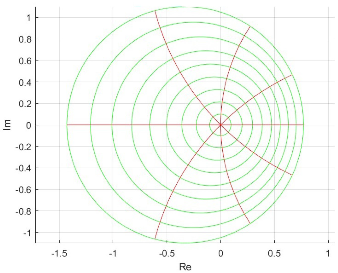
2. Definition and Visualization of the Class ${\Im }_{\mathfrak{G}}^{\Sigma }(\mathit{d},\mathit{\alpha },\mathit{\mu })$

Motivated by the previous constructions, we now introduce a new subclass of $\Sigma$ by employing subordination techniques involving Gregory coefficients, given by the series expansion in (1).

Definition 1. 

Let $\mathfrak{F}\in \Sigma$ have the form (4). The function $\mathfrak{F}$ is said to belong to the class ${\Im }_{\mathfrak{G}}^{\Sigma }(d,\alpha ,\mu )$ if it satisfies the following subordination conditions:

$$\begin{array}{cc}\hfill K\left(z\right)& :=(1-\alpha ){\displaystyle \frac{\mathfrak{F}\left(z\right)}{z}}+\alpha {\mathfrak{F}}^{\prime }\left(z\right){\left({\displaystyle \frac{(1-d)z}{\mathfrak{F}\left(z\right)-\mathfrak{F}\left(dz\right)}}\right)}^{\mu }\prec \mathfrak{G}\left(z\right),\hfill \end{array}$$

(9)

$$\begin{array}{cc}\hfill L\left(w\right)& :=(1-\alpha ){\displaystyle \frac{\mathfrak{g}\left(w\right)}{w}}+\alpha {\mathfrak{g}}^{\prime }\left(w\right){\left({\displaystyle \frac{(1-d)w}{\mathfrak{g}\left(w\right)-\mathfrak{g}\left(dw\right)}}\right)}^{\mu }\prec \mathfrak{G}\left(w\right),\hfill \end{array}$$

(10)

where $z,w\in \mathfrak{U}$, $d\in \mathbb{C}\setminus \left\{1\right\}$ with $\left|d\right|\le 1$, and parameters $\alpha \in [0,1]$ and $\mu \ge 0$. The inverse function $\mathfrak{g}\left(w\right)$ is understood to be ${\mathfrak{F}}^{-1}\left(w\right)$, consistent with the expansion given in (5).

Remark 1. 

The function $\mathfrak{G}$ is analytic in $\mathfrak{U}$ and satisfies the conditions $\Re \left(\mathfrak{G}\left(z\right)\right)>0$, $\mathfrak{G}\left(0\right)=1$, and ${\mathfrak{G}}^{\prime }\left(0\right)>0$. Furthermore, $\mathfrak{G}\left(z\right)$ maps the unit disk $\mathfrak{U}$ onto a region that is starlike with respect to 1 and symmetric with respect to the real axis [63]. This behavior is illustrated in Figure 1, generated with MATLAB R2024a software.

To better understand the domain $\mathfrak{U}$ in which the functions are defined, we include Figure 2 below, representing the unit disk. The plot was generated using MATLAB R2024a with a 2D grid representation.

It is important to note that the class ${\Im }_{\mathfrak{G}}^{\Sigma }(d,\alpha ,\mu )$ is non-empty. As a specific example, consider the function

$${\mathfrak{F}}_0\left(z\right)={\displaystyle \frac{z}{1-az}},\left|a\right|\le 1,$$

which clearly belongs to the class $\mathcal{S}$ and thus also to $\Sigma$. Its inverse is given by

$${\mathfrak{F}}_0^{-1}\left(w\right)={\mathfrak{g}}_0\left(w\right)={\displaystyle \frac{w}{1+aw}},\left|a\right|\le 1.$$

For instance, by choosing $a=0.3$, the images of the unit disk $\mathfrak{U}$ under the mappings ${\mathfrak{F}}_0$ and ${\mathfrak{g}}_0$ are shown in Figure 3 and Figure 4, respectively. These visualizations were generated using MATLAB R2024a grid plots.

Moreover, evaluating the functions defined in (9) and (10) for this particular choice of ${\mathfrak{F}}_0$ and ${\mathfrak{g}}_0$, yields the identity

$$K(-az)=L\left(az\right),\mathrm{for}\mathrm{all}z\in \mathfrak{U},$$

which confirms that the images of the mappings coincide, that is, $K\left(\mathfrak{U}\right)=L\left(\mathfrak{U}\right)$.

To further illustrate the behavior of the class ${\Im }_{\mathfrak{G}}^{\Sigma }(d,\alpha ,\mu )$, we set $\alpha =0.1$, $a=0.3$, and $\mu =1.001$. Using MATLAB R2024a, we generate 2D plots of the mappings K, L, and $\mathfrak{G}$ over the open unit disk $\mathfrak{U}$. The resulting images, shown in Figure 5 and Figure 6, clearly delineate the boundaries of the transformed regions.

Given that $\mathfrak{G}$ is univalent in $\mathfrak{U}$ and that $K\left(0\right)=L\left(0\right)=\mathfrak{G}\left(0\right)$, we observe that the subordinations

$$K\left(z\right)\prec \mathfrak{G}\left(z\right)\mathrm{and}L\left(w\right)\prec \mathfrak{G}\left(w\right)$$

are satisfied. Furthermore, as shown in Figure 7, the inclusion

$$K\left(\mathfrak{U}\right)=L\left(\mathfrak{U}\right)\subset \mathfrak{G}\left(\mathfrak{U}\right)$$

is visually confirmed.

Remark 2. 

For $\alpha =1$ and $\mu =0$, we obtain the class

$${\Im }_{\mathfrak{G}}^{\Sigma }(0,1,1)={\mathfrak{HS}}_{\Sigma },$$

defined as

The class ${\mathfrak{HS}}_{\Sigma }$, defined by

$${\mathfrak{HS}}_{\Sigma }=\left\{\mathfrak{F}\in \Sigma :{\mathfrak{F}}^{\prime }\left(z\right)\prec \mathfrak{G}\left(z\right)\mathrm{and}{\mathfrak{g}}^{\prime }\left(w\right)\prec \mathfrak{G}\left(w\right)\right\},$$

 was first introduced by Murugusundaramoorthy et al. in Definition 1 on page 3 of [63].

Remark 3. 

Similarly, setting $\alpha =1$, $d=0$, and $\mu =0$, we obtain

$${\Im }_{\mathfrak{G}}^{\Sigma }(0,1,0)=S_T^{*}\left(\lambda \right),$$

 where the class $S_T^{*}\left(\lambda \right)$ is given by

$$S_T^{*}\left(\lambda \right)=\left\{\mathfrak{F}\in \mathcal{S}:{\displaystyle \frac{z{\mathfrak{F}}^{\prime }\left(z\right)}{\mathfrak{F}\left(z\right)}}\prec \mathfrak{G}\left(z\right)\right\},$$

(11)

 as defined in [64] (p. 3).

For specific values of the parameters, we obtain the following new classes that have not been studied previously:

• For $\alpha =1$, the subclass ${\Im }_{\mathfrak{G}}^{\Sigma }(d,1,\mu )$ is defined by:

  $${\Im }_{\mathfrak{G}}^{\Sigma }(d,1,\mu )=\left\{\begin{array}{c}{\mathfrak{F}}^{\prime }\left(z\right){\left({\displaystyle \frac{(1-d)z}{\mathfrak{F}\left(z\right)-\mathfrak{F}\left(dz\right)}}\right)}^{\mu }\prec \mathfrak{G}\left(z\right),\hfill \\ {\mathfrak{g}}^{\prime }\left(w\right){\left({\displaystyle \frac{(1-d)w}{\mathfrak{g}\left(w\right)-\mathfrak{g}\left(dw\right)}}\right)}^{\mu }\prec \mathfrak{G}\left(w\right)\hfill \end{array}\right\}.$$
• For $\alpha =0$, the subclass ${\Im }_{\mathfrak{G}}^{\Sigma }(d,0,\mu )$ simplifies to:

  $${\Im }_{\mathfrak{G}}^{\Sigma }(d,0,\mu )=\left\{\begin{array}{c}{\displaystyle \frac{\mathfrak{F}\left(z\right)}{z}}\prec \mathfrak{G}\left(z\right),\hfill \\ {\displaystyle \frac{\mathfrak{g}\left(w\right)}{w}}\prec \mathfrak{G}\left(w\right)\hfill \end{array}\right\}.$$
• For $\alpha =\mu =1$, the subclass ${\Im }_{\mathfrak{G}}^{\Sigma }(d,1,1)$ takes the form:

  $${\Im }_{\mathfrak{G}}^{\Sigma }(d,1,1)=\left\{\begin{array}{c}{\displaystyle \frac{(1-d)z{\mathfrak{F}}^{\prime }\left(z\right)}{\mathfrak{F}\left(z\right)-\mathfrak{F}\left(dz\right)}}\prec \mathfrak{G}\left(z\right),\hfill \\ {\displaystyle \frac{(1-d)w{\mathfrak{g}}^{\prime }\left(w\right)}{\mathfrak{g}\left(w\right)-\mathfrak{g}\left(dw\right)}}\prec \mathfrak{G}\left(w\right)\hfill \end{array}\right\}.$$
• For $d=0$, the subclass ${\Im }_{\mathfrak{G}}^{\Sigma }(0,\alpha ,\mu )$ takes the form:

  $${\Im }_{\mathfrak{G}}^{\Sigma }(0,\alpha ,\mu )=\left\{\begin{array}{c}(1-\alpha ){\displaystyle \frac{\mathfrak{F}\left(z\right)}{z}}+\alpha {\mathfrak{F}}^{\prime }\left(z\right){\left({\displaystyle \frac{z}{\mathfrak{F}\left(z\right)}}\right)}^{\mu }\prec \mathfrak{G}\left(z\right),\hfill \\ (1-\alpha ){\displaystyle \frac{\mathfrak{g}\left(w\right)}{w}}+\alpha {\mathfrak{g}}^{\prime }\left(w\right){\left({\displaystyle \frac{w}{\mathfrak{g}\left(w\right)}}\right)}^{\mu }\prec \mathfrak{G}\left(w\right)\hfill \end{array}\right\}.$$
• For $d=0$ and $\alpha =1$, the subclass ${\Im }_{\mathfrak{G}}^{\Sigma }(0,1,\mu )$ reduces to:

  $${\Im }_{\mathfrak{G}}^{\Sigma }(0,1,\mu )=\left\{\begin{array}{c}{\mathfrak{F}}^{\prime }\left(z\right){\left({\displaystyle \frac{z}{\mathfrak{F}\left(z\right)}}\right)}^{\mu }\prec \mathfrak{G}\left(z\right),\hfill \\ {\mathfrak{g}}^{\prime }\left(w\right){\left({\displaystyle \frac{w}{\mathfrak{g}\left(w\right)}}\right)}^{\mu }\prec \mathfrak{G}\left(w\right)\hfill \end{array}\right\}.$$
• For $d=-1$, the subclass ${\Im }_{\mathfrak{G}}^{\Sigma }(-1,\alpha ,\mu )$ takes the form:

  $${\Im }_{\mathfrak{G}}^{\Sigma }(-1,\alpha ,\mu )=\left\{\begin{array}{c}(1-\alpha ){\displaystyle \frac{\mathfrak{F}\left(z\right)}{z}}+\alpha {\mathfrak{F}}^{\prime }\left(z\right){\left({\displaystyle \frac{-2z}{\mathfrak{F}\left(z\right)-\mathfrak{F}(-z)}}\right)}^{\mu }\prec \mathfrak{G}\left(z\right),\hfill \\ (1-\alpha ){\displaystyle \frac{\mathfrak{g}\left(w\right)}{w}}+\alpha {\mathfrak{g}}^{\prime }\left(w\right){\left({\displaystyle \frac{-2w}{\mathfrak{g}\left(w\right)-\mathfrak{g}(-w)}}\right)}^{\mu }\prec \mathfrak{G}\left(w\right)\hfill \end{array}\right\}.$$
• For $d=-1$ and $\alpha =1$, the subclass ${\Im }_{\mathfrak{G}}^{\Sigma }(-1,1,\mu )$ reduces to

  $${\Im }_{\mathfrak{G}}^{\Sigma }(-1,1,\mu )=\left\{\begin{array}{c}\mathfrak{F}\in \Sigma :{\mathfrak{F}}^{\prime }\left(z\right){\left({\displaystyle \frac{-2z}{\mathfrak{F}\left(z\right)-\mathfrak{F}(-z)}}\right)}^{\mu }\prec \mathfrak{G}\left(z\right),\hfill \\ {\mathfrak{g}}^{\prime }\left(w\right){\left({\displaystyle \frac{-2w}{\mathfrak{g}\left(w\right)-\mathfrak{g}(-w)}}\right)}^{\mu }\prec \mathfrak{G}\left(w\right)\hfill \end{array}\right\}.$$
• For $d=-1$ and $\alpha =1$, the subclass ${\Im }_{\mathfrak{G}}^{\Sigma }(-1,1,\mu )$ reduces to:

  $${\Im }_{\mathfrak{G}}^{\Sigma }(-1,1,\mu )=\left\{\begin{array}{c}{\mathfrak{F}}^{\prime }\left(z\right){\left({\displaystyle \frac{-2z}{\mathfrak{F}\left(z\right)-\mathfrak{F}(-z)}}\right)}^{\mu }\prec \mathfrak{G}\left(z\right),\hfill \\ {\mathfrak{g}}^{\prime }\left(w\right){\left({\displaystyle \frac{-2w}{\mathfrak{g}\left(w\right)-\mathfrak{g}(-w)}}\right)}^{\mu }\prec \mathfrak{G}\left(w\right)\hfill \end{array}\right\}.$$
• For $d=-1$ and $\mu =0$, the subclass ${\Im }_{\mathfrak{G}}^{\Sigma }(-1,\alpha ,0)$ reduces to:

  $${\Im }_{\mathfrak{G}}^{\Sigma }(-1,\alpha ,0)=\left\{\begin{array}{c}{\displaystyle \frac{\mathfrak{F}\left(z\right)}{z}}\prec \mathfrak{G}\left(z\right),\hfill \\ {\displaystyle \frac{\mathfrak{g}\left(w\right)}{w}}\prec \mathfrak{G}\left(w\right)\hfill \end{array}\right\}.$$
• For $d=-1$, $\mu =0$, and general $\alpha$, the subclass ${\Im }_{\mathfrak{G}}^{\Sigma }(-1,\alpha ,0)$ also takes the same form:

  $${\Im }_{\mathfrak{G}}^{\Sigma }(-1,\alpha ,0)=\left\{\begin{array}{c}{\displaystyle \frac{\mathfrak{F}\left(z\right)}{z}}\prec \mathfrak{G}\left(z\right),\hfill \\ {\displaystyle \frac{\mathfrak{g}\left(w\right)}{w}}\prec \mathfrak{G}\left(w\right)\hfill \end{array}\right\}.$$

Lemma 1 

([69,70]). Assume that $p\in \mathcal{P}$ and $p\left(z\right)$ is given by the expansion (6). Then, for all $n\in \mathbb{N}$, the following inequality holds:

$$|p_n|\le 2.$$

(12)

Sharpness holds true for the function

$$\mathfrak{F}\left(z\right)={\displaystyle \frac{1+z}{1-z}}.$$

The inequality (12) corresponds to the classical Carathéodory result (see [69,70]).

The following lemma builds upon the estimate derived in Lemma 6 and stated explicitly as Lemma 7 in [71], providing a useful tool for bounding complex expressions in our context:

Lemma 2 

([71], Lemma 7, p. 2). Assume that $r,s\in \mathbb{R}$ and $z_1,z_2\in \mathbb{C}$. If $\left|z_1\right|<T$ and $\left|z_2\right|<T$, then

$$\left|(r+s)z_1+(r-s)z_2\right|\le \left\{\begin{array}{ccc}2\left|r\right|T,& \mathit{for}& \left|r\right|\ge \left|s\right|,\\ 2\left|s\right|T,& \mathit{for}& \left|r\right|\le \left|s\right|.\end{array}\right.$$

(13)

Next, we establish upper bound estimates for the initial coefficients $|a_2|$ and $|a_3|$ of functions belonging to the class ${\Im }_{\mathfrak{G}}^{\Sigma }(d,\alpha ,\mu )$. These results are derived by employing the previously stated lemmas, together with the subordination conditions that define the class.

3. Main Results

Let the function $\mathfrak{F}\in \mathcal{A}$ be of the form (4). It is straightforward to verify that

$${\displaystyle \frac{\mathfrak{F}\left(z\right)-\mathfrak{F}\left(dz\right)}{1-d}}=z+\sum _{n=2}^{\infty }{\delta }_n{a}_n{z}^n,z\in \mathfrak{U},$$

where

$${\delta }_n={\displaystyle \frac{1-d^n}{1-d}}=\sum _{k=0}^{n-1}{d}^k,n\in \mathbb{N}.$$

(14)

Consequently, for any $\mu \ge 0$, we obtain the following expansion:

$${\left({\displaystyle \frac{(1-d)z}{\mathfrak{F}\left(z\right)-\mathfrak{F}\left(dz\right)}}\right)}^{\mu }=1-\mu {\delta }_2{a}_{2}z+\mu \left({\displaystyle \frac{1+\mu }{2}}{\delta }_2^2{a}_2^2-{\delta }_3{a}_3\right)z^2+\cdots .$$

Throughout this work, the parameters $\mu$ and d are assumed to satisfy the following conditions:

$$\mu {\delta }_n\ne n,\mu {\delta }_n<n\mathrm{for}\mathrm{all}n\ge 2,\mathrm{and}d\ne 1,\left|d\right|\le 1.$$

We now proceed to derive upper bound estimates for the initial coefficients $|a_2|$ and $|a_3|$ for functions belonging to the class ${\Im }_{\mathfrak{G}}^{\Sigma }(d,\alpha ,\mu )$.

Theorem 1. 

Let $\mathfrak{F}$, defined by (4), belong to the class ${\Im }_{\mathfrak{G}}^{\Sigma }(d,\alpha ,\mu )$. Then, the following coefficient bounds hold:

$$|a_2|\le min\left\{\mathcal{A}(\alpha ,\mu ,{\delta }_2,{\delta }_3),\mathcal{B}(\alpha ,\mu ,{\delta }_2)\right\},\left|a_3\right|\le min\left\{\mathcal{C}(\alpha ,\mu ,{\delta }_2,{\delta }_3),\mathcal{D}(\alpha ,\mu ,{\delta }_2,{\delta }_3)\right\},$$

 where

$$\begin{array}{cc}\hfill \mathcal{A}(\alpha ,\mu ,{\delta }_2,{\delta }_3)& =\sqrt{{\displaystyle \frac{3}{\left|6(1+2\alpha -\alpha \mu {\delta }_3)-3\alpha \mu (4-(1+\mu ){\delta }_2){\delta }_2+14{(1+\alpha -\alpha \mu {\delta }_2)}^2\right|}}},\hfill \\ \hfill \mathcal{B}(\alpha ,\mu ,{\delta }_2)& ={\displaystyle \frac{1}{2\left|1+\alpha -\alpha \mu {\delta }_2\right|}},\hfill \\ \hfill \mathcal{C}(\alpha ,\mu ,{\delta }_2,{\delta }_3)& ={\displaystyle \frac{1}{4{\left|1+\alpha -\alpha \mu {\delta }_2\right|}^2}}+{\displaystyle \frac{1}{2\left|1+2\alpha -\alpha \mu {\delta }_3\right|}},\hfill \\ \hfill \mathcal{D}(\alpha ,\mu ,{\delta }_2,{\delta }_3)& ={\left[min\left\{\mathcal{A},\mathcal{B}\right\}\right]}^2+{\displaystyle \frac{1}{2\left|1+2\alpha -\alpha \mu {\delta }_3\right|}}.\hfill \end{array}$$

These bounds are valid for $0\le \alpha \le 1$, $\mu \ge 0$, and $d\in \mathbb{C}\setminus \left\{1\right\}$ with $\left|d\right|\le 1$.

Proof.  

Since $\mathfrak{F}\in {\Im }_{\mathfrak{G}}^{\Sigma }(d,\alpha ,\mu )$, by Definition 1 and the subordination condition (9), there exists a Schwarz function $\mathcal{X}$ analytic in $\mathfrak{U}$ such that

$$\mathcal{X}\left(0\right)=0\mathrm{and}\left|\mathcal{X}\right(z\left)\right|<1,z\in \mathfrak{U}.$$

Under these conditions, we have

$$(1-\alpha ){\displaystyle \frac{\mathfrak{F}\left(z\right)}{z}}+\alpha {\mathfrak{F}}^{\prime }\left(z\right){\left({\displaystyle \frac{(1-d)z}{\mathfrak{F}\left(z\right)-\mathfrak{F}\left(dz\right)}}\right)}^{\mu }=\mathfrak{G}\left(\mathcal{X}\left(z\right)\right)={\displaystyle \frac{\mathcal{X}\left(z\right)}{ln(1+\mathcal{X}(z\left)\right)}}.$$

(15)

Therefore, the function

$$p\left(z\right):={\displaystyle \frac{1+\mathcal{X}\left(z\right)}{1-\mathcal{X}\left(z\right)}}=1+p_{1}z+p_2{z}^2+\cdots ,z\in \mathfrak{U},$$

(16)

belongs to the Carathéodory class $\mathcal{P}$. Solving for $\mathcal{X}\left(z\right)$ from (16), we obtain the expansion

$$\mathcal{X}\left(z\right)={\displaystyle \frac{p_1}{2}}z+{\displaystyle \frac{1}{2}}\left(p_2-{\displaystyle \frac{p_1^2}{2}}\right)z^2+{\displaystyle \frac{1}{2}}\left(p_3-p_1{p}_2+{\displaystyle \frac{p_1^3}{4}}\right)z^3+\cdots ,z\in \mathfrak{U}.$$

(17)

Substituting (17) into the generating function $\mathfrak{G}\left(\mathcal{X}\left(z\right)\right)={\displaystyle \frac{\mathcal{X}\left(z\right)}{ln(1+\mathcal{X}(z\left)\right)}}$, we obtain the following expansion:

$$\begin{array}{cc}\hfill \mathfrak{G}\left(\mathcal{X}\right(z\left)\right)& =1+{\displaystyle \frac{p_1}{4}}z+{\displaystyle \frac{1}{48}}(-7p_1^2+12p_2)z^2\hfill \\ \hfill & +{\displaystyle \frac{1}{192}}(17p_1^3-56p_1{p}_2+48p_3)z^3+\cdots .\hfill \end{array}$$

Similarly, since $\mathfrak{F}\in {\Im }_{\mathfrak{G}}^{\Sigma }(d,\alpha ,\mu )$, there exists another Schwarz function $\mathcal{Y}$ analytic in $\mathfrak{U}$, satisfying

$$\mathcal{Y}\left(0\right)=0\mathrm{and}\left|\mathcal{Y}\right(w\left)\right|<1,w\in \mathfrak{U}.$$

Under these conditions, the following subordination relation holds:

$$(1-\alpha ){\displaystyle \frac{\mathfrak{g}\left(w\right)}{w}}+\alpha {\mathfrak{g}}^{\prime }\left(w\right){\left({\displaystyle \frac{(1-d)w}{\mathfrak{g}\left(w\right)-\mathfrak{g}\left(dw\right)}}\right)}^{\mu }=\mathfrak{G}\left(\mathcal{Y}\left(w\right)\right)={\displaystyle \frac{\mathcal{Y}\left(w\right)}{ln(1+\mathcal{Y}(w\left)\right)}}.$$

(18)

Thus, the function

$$q\left(w\right)={\displaystyle \frac{1+\mathcal{Y}\left(w\right)}{1-\mathcal{Y}\left(w\right)}}=1+q_{1}w+q_2{w}^2+\cdots ,w\in \mathfrak{U},$$

(19)

belongs to the class $\mathcal{P}$. Expressing $\mathcal{Y}\left(w\right)$ in terms of $q\left(w\right)$ from (19), we obtain

$$\mathcal{Y}\left(w\right)={\displaystyle \frac{q_1}{2}}w+{\displaystyle \frac{1}{2}}\left(q_2-{\displaystyle \frac{q_1^2}{2}}\right)w^2+{\displaystyle \frac{1}{2}}\left(q_3-q_1{q}_2+{\displaystyle \frac{q_1^3}{4}}\right)w^3+\cdots ,w\in \mathfrak{U}.$$

(20)

Substituting (20) into the expansion of $\mathfrak{G}\left(\mathcal{Y}\left(w\right)\right)={\displaystyle \frac{\mathcal{Y}\left(w\right)}{ln(1+\mathcal{Y}(w\left)\right)}}$, we obtain

$$\begin{array}{cc}\hfill \mathfrak{G}\left(\mathcal{Y}\right(w\left)\right)& =1+{\displaystyle \frac{q_1}{4}}w+{\displaystyle \frac{1}{48}}\left(-7q_1^2+12q_2\right)w^2\hfill \\ \hfill & +{\displaystyle \frac{1}{192}}\left(17q_1^3-56q_1{q}_2+48q_3\right)w^3+\cdots .\hfill \end{array}$$

Combining expansions from Equations (15) and (18), we obtain

$$\begin{array}{cc}\hfill (1-\alpha ){\displaystyle \frac{\mathfrak{F}\left(z\right)}{z}}+\alpha {\mathfrak{F}}^{\prime }\left(z\right){\left({\displaystyle \frac{(1-d)z}{\mathfrak{F}\left(z\right)-\mathfrak{F}\left(dz\right)}}\right)}^{\mu }& =1+{\displaystyle \frac{p_1}{4}}z+{\displaystyle \frac{1}{48}}\left(-7p_1^2+12p_2\right)z^2\hfill \\ \hfill & +{\displaystyle \frac{1}{192}}\left(17p_1^3-56p_1{p}_2+48p_3\right)z^3+\cdots .\hfill \end{array}$$

(21)

$$\begin{array}{cc}\hfill (1-\alpha ){\displaystyle \frac{\mathfrak{g}\left(w\right)}{w}}+\alpha {\mathfrak{g}}^{\prime }\left(w\right){\left({\displaystyle \frac{(1-d)w}{\mathfrak{g}\left(w\right)-\mathfrak{g}\left(dw\right)}}\right)}^{\mu }& =1+{\displaystyle \frac{q_1}{4}}w+{\displaystyle \frac{1}{48}}\left(-7q_1^2+12q_2\right)w^2\hfill \\ \hfill & +{\displaystyle \frac{1}{192}}\left(17q_1^3-56q_1{q}_2+48q_3\right)w^3+\cdots .\hfill \end{array}$$

(22)

Conversely, the following expansion holds:

$$\begin{array}{cc}\hfill (1-\alpha ){\displaystyle \frac{\mathfrak{F}\left(z\right)}{z}}+\alpha {\mathfrak{F}}^{\prime }\left(z\right){\left({\displaystyle \frac{(1-d)z}{\mathfrak{F}\left(z\right)-\mathfrak{F}\left(dz\right)}}\right)}^{\mu }& =1+\left(1+\alpha -\alpha \mu {\delta }_2\right)a_{2}z\hfill \\ \hfill & +[\left(1+2\alpha -\alpha \mu {\delta }_3\right)a_3\hfill \\ \hfill & -\alpha \mu \left(2-{\displaystyle \frac{1}{2}}(1+\mu ){\delta }_2\right){\delta }_2{a}_2^2]z^2+\cdots .\hfill \end{array}$$

(23)

Similarly, we have:

$$\begin{array}{cc}\hfill (1-\alpha ){\displaystyle \frac{\mathfrak{g}\left(w\right)}{w}}+\alpha {\mathfrak{g}}^{\prime }\left(w\right){\left({\displaystyle \frac{(1-d)w}{\mathfrak{g}\left(w\right)-\mathfrak{g}\left(dw\right)}}\right)}^{\mu }& =1-\left(1+\alpha -\alpha \mu {\delta }_2\right)a_{2}w\hfill \\ \hfill & +[\left(1+2\alpha -\alpha \mu {\delta }_3\right)(2a_2^2-a_3)\hfill \\ \hfill & -\alpha \mu \left(2-{\displaystyle \frac{1}{2}}(1+\mu ){\delta }_2\right){\delta }_2{a}_2^2]w^2+\cdots .\hfill \end{array}$$

(24)

Comparing the corresponding coefficients in expansions (21) and (23), and also in (22) and (24), we obtain the following relations:

$$\begin{array}{cc}\hfill \left(1+\alpha -\alpha \mu {\delta }_2\right)a_2& ={\displaystyle \frac{p_1}{4}},\hfill \end{array}$$

(25)

$$\begin{array}{cc}\hfill \left(1+2\alpha -\alpha \mu {\delta }_3\right)a_3-\alpha \mu \left(2-{\displaystyle \frac{1}{2}}(1+\mu ){\delta }_2\right){\delta }_2{a}_2^2& ={\displaystyle \frac{1}{4}}\left(p_2-{\displaystyle \frac{7}{12}}{p}_1^2\right),\hfill \end{array}$$

(26)

$$\begin{array}{cc}\hfill \left(1+\alpha -\alpha \mu {\delta }_2\right)a_2& =-{\displaystyle \frac{q_1}{4}},\hfill \end{array}$$

(27)

and

$$\left(1+2\alpha -\alpha \mu {\delta }_3\right)(2a_2^2-a_3)-\alpha \mu \left(2-{\displaystyle \frac{1+\mu }{2}}{\delta }_2\right){\delta }_2{a}_2^2={\displaystyle \frac{1}{4}}\left(q_2-{\displaystyle \frac{7}{12}}{q}_1^2\right).$$

(28)

From Equations (25) and (27), we deduce:

$$p_1=-q_1,$$

(29)

and consequently,

$$a_2^2={\displaystyle \frac{p_1^2+q_1^2}{32{\left(1+\alpha -\alpha \mu {\delta }_2\right)}^2}}.$$

(30)

Adding Equations (26) and (28), we obtain:

$$\left[2(1+2\alpha -\alpha \mu {\delta }_3)-\alpha \mu (4-(1+\mu ){\delta }_2){\delta }_2\right]a_2^2={\displaystyle \frac{1}{4}}(p_2+q_2)-{\displaystyle \frac{7}{48}}(p_1^2+q_1^2).$$

(31)

Substituting the expression from (30) into (31) gives:

$$a_2^2={\displaystyle \frac{3(p_2+q_2)}{4\left[6(1+2\alpha -\alpha \mu {\delta }_3)-3\alpha \mu (4-(1+\mu ){\delta }_2){\delta }_2+14{(1+\alpha -\alpha \mu {\delta }_2)}^2\right]}}.$$

(32)

Now, by applying the bound from (12) and using the triangle inequality in (32), we obtain:

$$|a_2|\le \sqrt{{\displaystyle \frac{3}{\left|6(1+2\alpha -\alpha \mu {\delta }_3)-3\alpha \mu (4-(1+\mu ){\delta }_2){\delta }_2+14{(1+\alpha -\alpha \mu {\delta }_2)}^2\right|}}}=:\mathcal{A}(\alpha ,\mu ,{\delta }_2,{\delta }_3).$$

In addition, applying the estimate from (12) to Equation (25) leads to the simpler bound:

$$\left|a_2\right|\le {\displaystyle \frac{1}{2\left|1+\alpha -\alpha \mu {\delta }_2\right|}}:=\mathcal{B}(\alpha ,\mu ,{\delta }_2).$$

Furthermore, by subtracting Equation (28) from (26), we obtain:

$$2\left(1+2\alpha -\alpha \mu {\delta }_3\right)(a_3-a_2^2)={\displaystyle \frac{p_2-q_2}{4}}-{\displaystyle \frac{7}{48}}(p_1^2-q_1^2).$$

(33)

$$a_3={\displaystyle \frac{p_1^2+q_1^2}{32{\left(1+\alpha -\alpha \mu {\delta }_2\right)}^2}}+{\displaystyle \frac{p_2-q_2}{8\left(1+2\alpha -\alpha \mu {\delta }_3\right)}}.$$

(34)

By applying the bound from (12) and using the triangle inequality in (34), we derive the estimate:

$$\left|a_3\right|\le {\displaystyle \frac{1}{4{\left|1+\alpha -\alpha \mu {\delta }_2\right|}^2}}+{\displaystyle \frac{1}{2\left|1+2\alpha -\alpha \mu {\delta }_3\right|}}:=\mathcal{C}(\alpha ,\mu ,{\delta }_2,{\delta }_3).$$

Alternatively, using Equation (30), relation (34) can be rewritten as:

$$a_3=a_2^2+{\displaystyle \frac{p_2-q_2}{8\left(1+2\alpha -\alpha \mu {\delta }_3\right)}}.$$

(35)

Applying the triangle inequality in conjunction with (12), and taking into account that

$$\left|a_2\right|\le min\left\{\mathcal{A}(\alpha ,\mu ,{\delta }_2,{\delta }_3),\mathcal{B}(\alpha ,\mu ,{\delta }_2)\right\},$$

we obtain the estimate

$$\left|a_3\right|\le {\left[min\left\{\mathcal{A}(\alpha ,\mu ,{\delta }_2,{\delta }_3),\mathcal{B}(\alpha ,\mu ,{\delta }_2)\right\}\right]}^2+{\displaystyle \frac{1}{2\left|1+2\alpha -\alpha \mu {\delta }_3\right|}}:=\mathcal{D}(\alpha ,\mu ,{\delta }_2,{\delta }_3).$$

(36)

This completes the proof. □

We now derive the Fekete–Szegö inequalities for functions belonging to the class ${\Im }_{\mathfrak{G}}^{\Sigma }(d,\alpha ,\mu )$ as introduced in Definition 1.

Theorem 2. 

Assume that $\mathfrak{F}\in {\Im }_{\mathfrak{G}}^{\Sigma }(d,\alpha ,\mu )$ and let $\varrho \in \mathbb{R}$. In this case, the following Fekete–Szegö inequality holds:

$$\left|a_3-\varrho a_2^2\right|\le \left\{\begin{array}{cc}{\displaystyle \frac{1}{2\left|1+2\alpha -\alpha \mu {\delta }_3\right|}},\hfill & \mathit{if}\left|\mathcal{T}\left(\varrho \right)\right|\le {\displaystyle \frac{1}{8\left(1+2\alpha -\alpha \mu {\delta }_3\right)}},\hfill \\ 4\left|\mathcal{T}\left(\varrho \right)\right|,\hfill & \mathit{if}\left|\mathcal{T}\left(\varrho \right)\right|\ge {\displaystyle \frac{1}{8\left(1+2\alpha -\alpha \mu {\delta }_3\right)}}.\hfill \end{array}\right.$$

Here, the function $\mathcal{T}\left(\varrho \right)$ is defined as:

$$\mathcal{T}\left(\varrho \right)={\displaystyle \frac{3(1-\varrho )}{4\left[6\left(1+2\alpha -\alpha \mu {\delta }_3\right)-3\alpha \mu \left(4-(1+\mu ){\delta }_2\right){\delta }_2+14{\left(1+\alpha -\alpha \mu {\delta }_2\right)}^2\right]}}.$$

Proof.  

Using (32) and (35), we obtain:

$$\begin{array}{cc}\hfill a_3-\varrho a_2^2& ={\displaystyle \frac{3(1-\varrho )(p_2+q_2)}{4\left[6(1+2\alpha -\alpha \mu {\delta }_3)-3\alpha \mu (4-(1+\mu ){\delta }_2){\delta }_2+14{(1+\alpha -\alpha \mu {\delta }_2)}^2\right]}}\hfill \\ \hfill & +{\displaystyle \frac{p_2-q_2}{8\left(1+2\alpha -\alpha \mu {\delta }_3\right)}}\hfill \\ \hfill & +\left[\mathcal{T}\left(\varrho \right)+{\displaystyle \frac{1}{8(1+2\alpha -\alpha \mu {\delta }_3)}}\right]p_2+\left[\mathcal{T}\left(\varrho \right)-{\displaystyle \frac{1}{8(1+2\alpha -\alpha \mu {\delta }_3)}}\right]q_2,\hfill \end{array}$$

For the definition of the function $\mathcal{T}\left(\varrho \right)$, see Theorem 2. Applying the triangle inequality and Lemma 2, we obtain the desired result. □

Obviously, by setting $d=0$ in (12), we observe that for $n\in \mathbb{N}$, the following holds:

$${\delta }_n=1.$$

Hence, by substituting $d=0$ into Theorems 1 and 2, we obtain the following remarks and example:

Remark 4. 

Choosing $\alpha =1$ and $\mu =0$, we have:

$$\left|a_2\right|\le \sqrt{{\displaystyle \frac{3}{74}}}\approx 0.0234\dots ,\left|a_3\right|\le {\displaystyle \frac{23}{111}}\approx 0.2072\dots ,$$

 and

$$\left|a_3-\varrho a_2^2\right|\le \left\{\begin{array}{cc}{\displaystyle \frac{1}{6}},\hfill & \mathit{if}\varrho \in \left[-\frac{28}{9},\frac{46}{9}\right],\hfill \\ {\displaystyle \frac{3\left|1-\varrho \right|}{74}},\hfill & \mathit{if}\varrho \in (-\infty ,-\frac{28}{9}]\cup [\frac{46}{9},\infty ).\hfill \end{array}\right.$$

This result coincides with Theorems 1 and 2 in [63].

Remark 5. 

Choosing $\alpha =\mu =1$, we have:

$$\left|a_2\right|\le 0.3872\dots ,\left|a_3\right|\le 0.4,$$

 and

$$\left|a_3-\varrho a_2^2\right|\le \left\{\begin{array}{cc}{\displaystyle \frac{1}{4}},\hfill & \mathit{if}\left|1-\varrho \right|\le \frac{5}{3},\hfill \\ {\displaystyle \frac{3\left|1-\varrho \right|}{20}},\hfill & \mathit{if}\left|1-\varrho \right|\ge \frac{5}{3}.\hfill \end{array}\right.$$

This result coincides with Example 1 in [63].

Example 1. 

Choosing $\alpha =\mu =0$ (or equivalently, $\alpha =0$ and $\mu =1$), we have:

$$\left|a_2\right|\le 0.3872\dots ,\left|a_3\right|\le 0.65,$$

 and

$$\left|a_3-\varrho a_2^2\right|\le \left\{\begin{array}{cc}{\displaystyle \frac{1}{2}},\hfill & \mathit{if}\left|1-\varrho \right|\le {\displaystyle \frac{10}{3}},\hfill \\ {\displaystyle \frac{3\left|1-\varrho \right|}{20}},\hfill & \mathit{if}\left|1-\varrho \right|\ge {\displaystyle \frac{10}{3}}.\hfill \end{array}\right.$$

Obviously, by setting $d=-1$ in Theorem 1 (see also the definition of ${\delta }_n$), we obtain:

$${\delta }_n=\left\{\begin{array}{cc}1,\hfill & \mathrm{if}n\mathrm{is}\mathrm{odd},\hfill \\ 0,\hfill & \mathrm{if}n\mathrm{is}\mathrm{even}.\hfill \end{array}\right.$$

Based on this, we consider two cases:

(i)

Applying $d=-1$ in Theorems 1 and 2 yields the following results for even values of n:

Example 2. 

For $\alpha =0$, we recover the same result as in Example 1.

Remark 6. 

For $\alpha =1$, the results coincide with those presented in Remark 5, which align with Theorems 1 and 2 in [63].

(ii)

Similarly, applying $d=-1$ in Theorems 1 and 2 yields the following results for odd values of n:

Example 3. 

For $\alpha =0$, we again obtain the same result as in Example 1.

Remark 7. 

For $\alpha =\mu =1$, the results coincide with those in Remark 6, matching Example 1 in [63].

Remark 8. 

For $\alpha =\mu =0$, the results are consistent with those presented in Remark 6, corresponding to Theorems 1 and 2 in [63].

4. Conclusions

In this study, we introduced and analyzed Gregory coefficients, examining their fundamental properties and demonstrating how specific parameter selections yield well-known mathematical sequences. We rigorously defined the class ${\Im }_{\mathfrak{G}}^{\Sigma }(d,\alpha ,\mu )$, providing illustrative examples and graphical representations to elucidate its structural characteristics.

A central focus of this work was the coefficient estimation problem within this class. By employing analytical methods, we derived bounds for the initial coefficients, thereby contributing to the broader study of bi-univalent functions and their coefficient constraints. Despite these advances, estimating higher-order coefficients remains an open challenge, offering a promising avenue for future research.

The application of subordination principles enabled the derivation of new results, underscoring the connection between Gregory coefficients and analytic function theory. These findings expand the applicability of Gregory coefficients in geometric function theory and establish a robust foundation for subsequent studies.

Future research directions include the following:

• Extending coefficient estimates to higher-order terms.
• Broadening the use of subordination techniques to other subclasses of analytic functions.
• Investigating additional subclasses within the bi-univalent function framework.
• Exploring the impact of graphical and geometric representations in establishing sharp inequalities.
• Applying the introduced class to convolution operators or integral transforms to study further analytic properties.

Moreover, incorporating numerical simulations and graphical visualizations could yield deeper insights into the geometric properties of these function classes. These findings not only enrich the theory of bi-univalent functions but also open new perspectives for their application in analytic approximation and geometric theory.

References

1. Jordan, C. The Calculus of Finite Differences; Chelsea Publishing Company: New York, NY, USA, 1947. [Google Scholar]
2. Comtet, L. Advanced Combinatorics, 2nd ed.; D. Reidel Publishing Company: Boston, MA, USA, 1974. [Google Scholar]
3. Davis, H.T. The approximation of logarithmic numbers. Amer. Math. Mon. 1957, 64, 11–18. [Google Scholar] [CrossRef]
4. Berezin, I.S.; Zhidkov, N.P. Computing Methods; Pergamon Press: Oxford, UK, 1965. [Google Scholar]
5. Phillips, G.M. Gregory’s Method for Numerical Integration. Am. Math. Mon. 1972, 79, 270–274. [Google Scholar] [CrossRef]
6. Qi, F.; Zhao, J.-L. Some Properties of the Bernoulli Numbers of the Second Kind and Their Generating Function. Bull. Korean Math. Soc. 2018, 55, 1909–1920. [Google Scholar] [CrossRef]
7. Blagouchine, I.V. Expansions of Generalized Euler’s Constants into the Series of Polynomials in π−2 and into the Formal Enveloping Series with Rational Coefficients Only. J. Number Theory 2016, 158, 365–396. [Google Scholar] [CrossRef]
8. Blagouchine, I.V. Three Notes on Ser’s and Hasse’s Representations for the Zeta-Functions. Integers 2018, 18, A4. Available online: https://math.colgate.edu/~integers/a4/a4.pdf (accessed on 9 May 2025).
9. Merlini, D.; Sprugnoli, R.; Verri, M.C. The Cauchy numbers. Discret. Math. 2006, 306, 1906–1920. [Google Scholar] [CrossRef]
10. Blagouchine, I.V. Two Series Expansions for the Logarithm of the Gamma Function Involving Stirling Numbers and Containing Only Rational Coefficients for Certain Arguments Related to π−1. J. Math. Anal. Appl. 2016, 442, 404–434. [Google Scholar] [CrossRef]
11. Liu, H.M.; Qi, S.H.; Ding, S.Y. Some recurrence relations for Cauchy numbers of the first kind. J. Integer Seq. 2010, 13, 10.2.3. [Google Scholar]
12. Nemes, G. An asymptotic expansion for the Bernoulli numbers of the second kind. J. Integer Seq. 2011, 14, 11.4.8. [Google Scholar]
13. Qi, F.; Zhang, X.-J. An integral representation, some inequalities, and complete monotonicity of Bernoulli numbers of the second kind. Bull. Korean Math. Soc. 2015, 52, 987–998. [Google Scholar] [CrossRef]
14. Young, P.T. A 2-adic formula for Bernoulli numbers of the second kind and for the Nörlund numbers. J. Number Theory 2008, 128, 2951–2962. [Google Scholar] [CrossRef]
15. Kowalenko, V. Properties and applications of the reciprocal logarithm numbers. Acta Appl. Math. 2010, 109, 413–437. [Google Scholar] [CrossRef]
16. Alabdulmohsin, I.M. Summability Calculus: A Comprehensive Theory of Fractional Finite Sums; Springer: Cham, Switzerland, 2018. [Google Scholar] [CrossRef]
17. Duren, P.L. Univalent Functions; Grundlehren der Mathematischen Wissenschaften; Springer: New York, NY, USA, 1983; Volume 259. [Google Scholar]
18. Lewin, M. On a Coefficient Problem for Bi-univalent Functions. Proc. Am. Math. Soc. 1967, 18, 63–68. [Google Scholar] [CrossRef]
19. Brannan, D.A.; Taha, T.S. On Some Classes of Bi-univalent Functions. Stud. Univ. Babeș-Bolyai Math. 1986, 31, 70–77. [Google Scholar]
20. Netanyahu, E. The Minimal Distance of the Image Boundary from the Origin and the Second Coefficient of a Univalent Function in |z|<1. Arch. Ration. Mech. Anal. 1969, 32, 100–112. [Google Scholar]
21. Tan, D.L. Coefficient Estimates for Bi-univalent Functions. Chin. Ann. Math. Ser. A 1984, 5, 559–568. [Google Scholar]
22. Akgül, A. Fekete–Szegö Variations for Some New Classes of Analytic Functions Explained over Poisson and Borel Distribution Series. Math. Methods Appl. Sci. 2025, 48, 9241–9252. [Google Scholar] [CrossRef]
23. Akgül, A. On a New Subclass of Bi-univalent Analytic Functions Characterized by (P, Q)-Lucas Polynomial Coefficients via Sălăgean Differential Operator. In Operators, Inequalities and Approximation: Theory and Applications; Tripathy, B.C., Paikray, S.K., Dutta, H., Jena, B.B., Eds.; Springer Nature: Singapore, 2024; pp. 159–182. [Google Scholar] [CrossRef]
24. Singh, G.; Singh, G.; Singh, G. Certain Subclasses of Sakaguchi-type Bi-univalent Functions. Ganita 2019, 69, 45–55. [Google Scholar]
25. Srivastava, H.M.; Mishra, A.K.; Gochhayat, P. Certain Subclasses of Analytic and Bi-univalent Functions. Appl. Math. Lett. 2010, 23, 1188–1192. [Google Scholar] [CrossRef]
26. Srivastava, H.M.; Wanas, A.K.; Güney, H.Ö. New Families of Bi-univalent Functions Associated with the Bazilevič Functions and the k-Pseudo-starlike Functions. Iran. J. Sci. Technol. Trans. A Sci. 2021, 45, 1799–1804. [Google Scholar] [CrossRef]
27. Altınkaya, Ş.; Yalçın, S. On the Chebyshev Polynomial Coefficient Problem of Some Subclasses of Bi-univalent Functions. Gulf J. Math. 2017, 5, 34–40. [Google Scholar] [CrossRef]
28. Srivastava, H.M.; Altınkaya, Ş.; Yalçın, S. Certain Subclasses of Bi-univalent Functions Associated with the Horadam Polynomials. Iran. J. Sci. Technol. Trans. A Sci. 2019, 43, 1873–1879. [Google Scholar] [CrossRef]
29. Lindelöf, E. Mémoire sur certaines inégalités dans la théorie des fonctions monogènes et sur quelques propriétés nouvelles de ces fonctions dans le voisinage d’un point singulier essentiel. Ann. Soc. Sci. Fenn. 1909, 35, 1–35. [Google Scholar]
30. Rogosinski, W.; Szegö, G. Über die Abschätzungen von Potenzreihen, die in einem Kreise beschränkt bleiben. Math. Z. 1928, 28, 73–94. [Google Scholar] [CrossRef]
31. Rogosinski, W. On the coefficients of subordinate functions. Proc. Lond. Math. Soc. 1943, 48, 48–82. [Google Scholar] [CrossRef]
32. Littlewood, J.E. Lectures on the Theory of Functions; Oxford University Press: Oxford, UK, 1944. [Google Scholar]
33. Robertson, M.S. Quasi-subordination and coefficient conjecture. Bull. Amer. Math. Soc. 1970, 76, 1–9. [Google Scholar] [CrossRef]
34. Goodman, A.W. Univalent Functions; Mariner Publishing Company Inc.: Tampa, FL, USA, 1983; Volume 1–2. [Google Scholar]
35. Pommerenke, C. Univalent Functions; Vandenhoeck & Ruprecht: Göttingen, Germany, 1975. [Google Scholar]
36. Ma, W.; Minda, D. A Unified Treatment of Some Special Classes of Univalent Functions. In Proceedings of the Conference on Complex Analysis; Li, Z., Ren, F., Yang, L., Zhang, S., Eds.; International Press: Vienna, Austria, 1994; pp. 157–169. [Google Scholar]
37. Nevanlinna, R.H. Über die konforme Abbildung von Sterngebieten. Översikt Vetenskaps-Soc. Förh./A 1921, 63, 1–21. [Google Scholar]
38. Goluzin, G.M. Geometric Theory of Functions of a Complex Variable; American Mathematical Society: Providence, RI, USA, 1969; Volume 26. (In Russian) [Google Scholar]
39. Sakaguchi, K. On a Certain Univalent Mapping. J. Math. Soc. Jpn. 1959, 11, 72–75. [Google Scholar] [CrossRef]
40. Owa, S.; Sekine, T.; Yamakawa, R. On Sakaguchi Type Functions. Appl. Math. Comput. 2007, 187, 356–361. [Google Scholar] [CrossRef]
41. Obradović, M. A Class of Univalent Functions. Hokkaido Math. J. 1998, 27, 329–335. [Google Scholar] [CrossRef]
42. Sharma, P.; Raina, R.K. On a Sakaguchi Type Class of Analytic Functions Associated with Quasi-subordination. Comment. Math. Univ. St. Pauli 2015, 64, 59–70. [Google Scholar]
43. Srivastava, H.M.; Hussain, S.; Raziq, A.; Raza, M. The Fekete–Szegö Functional for a Subclass of Analytic Functions Associated with Quasi-subordination. Carpathian J. Math. 2018, 34, 103–113. [Google Scholar] [CrossRef]
44. Kilar, N.; Şimşek, Y. Computational formulas and identities for new classes of Hermite-based Milne–Thomson type polynomials. Math. Meth. Appl. Sci. 2021, 44, 6731–6762. [Google Scholar] [CrossRef]
45. Kilar, N.; Kim, D.; Şimşek, Y. Formulae bringing to light from certain classes of numbers and polynomials. Rev. Real Acad. Cienc. Exactas Fís. Nat. Ser. A-Mat. 2023, 117, 27. [Google Scholar] [CrossRef]
46. Keogh, F.R.; Merkes, E.P. A Coefficient Inequality for Certain Classes of Analytic Functions. Proc. Am. Math. Soc. 1969, 20, 8–12. [Google Scholar] [CrossRef]
47. Szegő, G. Orthogonal Polynomials, 4th ed.; American Mathematical Society Colloquium Publications; American Mathematical Society: Providence, RI, USA, 1975; Volume 23. [Google Scholar]
48. Fekete, M.; Szegő, G. Eine Bemerkung über ungerade schlichte Funktionen. J. Lond. Math. Soc. 1933, 8, 85–89. [Google Scholar] [CrossRef]
49. Mohd, M.H.; Darus, M. Fekete–Szegö problems for quasi-subordination classes. Abstr. Appl. Anal. 2012, 2012, 192956. [Google Scholar] [CrossRef]
50. Kanas, S.; Darwish, H.E. Fekete–Szegö problem for starlike and convex functions of complex order. Appl. Math. Lett. 2010, 23, 777–782. [Google Scholar] [CrossRef]
51. Akgül, A.; Altınkaya, Ş. Coefficient Estimates Associated with a New Subclass of Bi-Univalent Functions. Acta Univ. Apulensis 2017, 52, 121–128. [Google Scholar] [CrossRef]
52. Akgül, A.; Sakar, F.M. A New Characterization of (P,Q)-Lucas Polynomial Coefficients of the Bi-Univalent Function Class Associated with the q-Analogue of Noor Integral Operator. Afr. Mat. 2022, 33, 87. [Google Scholar] [CrossRef]
53. Akgül, A.; Sakar, F.M. A Certain Subclass of Bi-univalent Analytic Functions Introduced by Means of the q-Analogue of Noor Integral Operator and Horadam Polynomials. Turk. J. Math. 2019, 43, 2275–2286. [Google Scholar] [CrossRef]
54. Abirami, C.; Magesh, N.; Yamini, J.; Kargar, R. Horadam Polynomial Coefficient Estimates for the Classes of α-Bi-Pseudo-Starlike and Bi-Bazilevič Functions. J. Anal. 2020, 28, 951–960. [Google Scholar] [CrossRef]
55. Patil, A.B.; Shaba, T.G. Sharp Initial Coefficient Bounds and the Fekete–Szegö Problem for Some Subclasses of Analytic and Bi-univalent Functions. Ukr. Math. J. 2023, 75, 225–234. [Google Scholar] [CrossRef]
56. Karthikeyan, K.R.; Mohankumar, D.; Breaz, D. A Comprehensive Class of Starlike Functions Involving Mittag–Leffler Function. Appl. Math. Sci. Eng. 2025, 33, 2487531. [Google Scholar] [CrossRef]
57. Abbas, M.; Alhefthi, R.K.; Breaz, D.; Arif, M. On Coefficient Inequalities for Functions of Symmetric Starlike Related to a Petal-Shaped Domain. Axioms 2025, 14, 165. [Google Scholar] [CrossRef]
58. Amourah, A.; Salleh, Z.; Frasin, B.A.; Khan, M.G.; Ahmad, B. Subclasses of Bi-univalent Functions Subordinate to Gegenbauer Polynomials. Afr. Mat. 2023, 34, 41. [Google Scholar] [CrossRef]
59. Cotîrlă, L.I.; Wanas, A.K. Coefficient-Related Studies and Fekete–Szegö Type Inequalities for New Classes of Bi-starlike and Bi-convex Functions. Symmetry 2022, 14, 2263. [Google Scholar] [CrossRef]
60. Murugusundaramoorthy, G.; Vijaya, K. Certain Subclasses of Analytic Functions Associated with Generalized Telephone Numbers. Symmetry 2022, 14, 1053. [Google Scholar] [CrossRef]
61. Orhan, H.; Masih, V.S.; Ebadian, A. Coefficient Estimates for Power Bi–univalent Ma–Minda Starlike and Derivative Functions. J. Anal. 2025. [Google Scholar] [CrossRef]
62. Oros, G.I.; Cotîrlă, L.I. Coefficient Estimates and the Fekete–Szegö Problem for New Classes of m-Fold Symmetric Bi-univalent Functions. Mathematics 2022, 10, 129. [Google Scholar] [CrossRef]
63. Murugusundaramoorthy, G.; Vijaya, K.; Bulboacă, T. Initial Coefficient Bounds for Bi-univalent Functions Related to Gregory Coefficients. Mathematics 2023, 11, 2857. [Google Scholar] [CrossRef]
64. Kazımoğlu, S.; Deniz, E.; Srivastava, H.M. Sharp Coefficient Bounds for Starlike Functions Associated with Gregory Coefficients. Complex Anal. Oper. Theory 2024, 18, 6. [Google Scholar] [CrossRef]
65. Panigrahi, T.; Jena, S.; El-Ashwah, R.M. Certain Properties of Bazilevič-Type Univalent Class Defined Through Subordination. Afr. Mat. 2024, 35, 75. [Google Scholar] [CrossRef]
66. Tang, H.; Mujahid, Z.; Khan, N.; Tchier, F.; Ghaffar Khan, M. Generalized Bounded Turning Functions Connected with Gregory Coefficients. Axioms 2024, 13, 359. [Google Scholar] [CrossRef]
67. Bulut, S. Faber polynomial coefficient estimates for analytic bi-univalent functions associated with Gregory coefficients. Korean J. Math. 2024, 32, 285–295. [Google Scholar] [CrossRef]
68. Srivastava, H.M.; Cho, N.E.; Alderremy, A.A.; Lupas, A.A.; Mahmoud, E.E.; Khan, S. Sharp inequalities for a class of novel convex functions associated with Gregory polynomials. J. Inequal. Appl. 2024, 2024, 140. [Google Scholar] [CrossRef]
69. Carathéodory, C. Über den Variabilitätsbereich der Koeffizienten von Potenzreihen, die Gegebene Werte Nicht Annehmen. Math. Ann. 1907, 64, 95–115. [Google Scholar] [CrossRef]
70. Carathéodory, C. Über den Variabilitätsbereich der Fourier’schen Konstanten von Positiven Harmonischen Funktionen. Rend. Circ. Mat. Palermo 1911, 32, 193–217. [Google Scholar] [CrossRef]
71. Zaprawa, P. Estimates of Initial Coefficients for Bi-univalent Functions. Abstr. Appl. Anal. 2014, 2014, 357480. [Google Scholar] [CrossRef]
Figure 1. 3D surface plot of the mapping under G ( z ) .
Symmetry 17 00884 g001
Figure 2. The unit disk U .
Symmetry 17 00884 g002
Figure 3. Image of U under F 0 ( z ) = z 1 a z , with a = 0.3 .
Symmetry 17 00884 g003
Figure 4. Image of U under g 0 ( w ) = w 1 + a w , with a = 0.3 .
Symmetry 17 00884 g004
Figure 5. Image of K ( U ) = L ( U ) .
Symmetry 17 00884 g005
Figure 6. Image of G ( U ) .
Symmetry 17 00884 g006
Figure 7. K ( U ) = L ( U ) G ( U ) .
Symmetry 17 00884 g007