Assessment of the Measured Mixing Time in a Water Model of Asymmetrical Gas-Stirred Ladle with a Low Gas Flowrate Part II: Effect of the Salt Solution Tracer Volume and Concentration

Abstract

Mixing time, as a key parameter for evaluating ladle refining efficiency, has long attracted extensive attention from researchers. In typical experimental studies, salt solution tracers are introduced into ladle water models to assess the degree of mixing within the ladle. Previous studies have demonstrated that the volume of tracer can significantly influence the measured mixing time. However, the gas flow rates employed in these studies are generally relatively high, whereas, in industrial operations, especially during final composition adjustments, lower gas flow rates are often applied. To systematically investigate the effect of the salt solution tracer volume on the mixing efficiency in a ladle water model under asymmetrical gas stirring with a low gas flow rate, a 1:3-scaled water model was developed based on a 130-ton industrial ladle. The mixing behaviors corresponding to different tracer volumes were comprehensively analyzed. The results indicate that the relationship between tracer volume and mixing time is non-monotonic. As the tracer volume increases, the mixing time first decreases and then increases, reaching a minimum at 185 mL. When the tracer volume was small, the dimensionless concentration curves at Monitoring Point 4 exhibited two distinct patterns: A parabolic profile, which was when the tracer initially moved through the left and central regions and then slowly crossed the gas plume to reach the monitoring point. A sinusoidal profile, which was when the tracer predominantly circulated along the right side of the ladle. When the tracer volume exceeded 277 mL, the concentration curves at Monitoring Point 4 consistently exhibited a sinusoidal pattern. Compared with moderate gas flow conditions (8.3 L/min), the peak concentration at Monitoring Point 3 was significantly lower under a low gas flow (2.3 L/min), and the overall mixing time was longer, indicating reduced mixing efficiency. Based on the findings, a recommended tracer volume range of 185–277 mL is proposed for low gas flow conditions (2.3 L/min) to achieve accurate and efficient mixing time measurements with minimal disturbance to the flow field. It was also observed that when the tracer concentration was relatively low, the mixing behavior throughout the ladle became more uniform.

1. Introduction

The ladle plays a crucial role in the secondary refining process of steelmaking [1,2,3,4,5]. Gas is injected into the molten pool through porous plugs installed at the ladle bottom, forming bubbles that rise through the melt. The circulating flow induced by bubble ascent provides several key metallurgical functions: (1) promoting homogenization of temperature and composition fields in the molten steel [6,7,8,9,10,11,12,13]; and (2) assisting in the removal of non-metallic inclusions through flotation and enhancing their removal efficiency [14,15,16]. Due to the difficulty of directly observing the internal flow characteristics of the ladle under industrial conditions, most scholars have employed physical modeling [17,18,19,20,21,22,23,24] and mathematical modeling [25,26,27,28,29,30,31,32,33,34] to investigate the flow homogenization [35,36,37,38] and inclusion behavior [39,40,41,42] inside the ladle. Due to the low stirring efficiency associated with central gas injection [43], asymmetric stirring is commonly employed in small-capacity ladles [44].

Among various performance indicators, the mixing time is a key parameter for evaluating ladle refining efficiency. Understanding the mixing time is essential for optimizing refining operations. It helps avoid insufficient stirring, which may lead to poor refining quality, and it also prevents over-stirring, which can accelerate refractory erosion. However, the measurement of mixing time is influenced by multiple factors. Classic studies have indicated that the injection location of the tracer and the position of the monitoring point significantly affect the measured mixing time [2,45,46]. Contrarily, Krishna et al. [47] demonstrated through optimized experimental design that, when properly measured, the mixing time is independent of tracer injection and sampling locations. Several researchers have examined the effects of the gas flow rate [48,49,50], slag layer properties [51,52,53,54], and the position and number of porous plugs [55,56,57,58,59,60] on the mixing and flow behavior in ladles. Notably, Renato et al. [61] found that lower gas flow rates can lead to shorter mixing times due to a more inclined primary recirculation loop, which enhances turbulent diffusion. In addition, the effect of slag on mixing time is dual in nature. Kim et al. [62] observed that the presence of a slag layer increases the mixing time, which becomes more pronounced with increasing slag thickness and viscosity. However, Han et al. [53] pointed out that, under extremely low gas flow rates, a low-density slag layer may actually reduce the mixing time.

Current methods for measuring the mixing time can be broadly categorized into two types: (1) invasive techniques, and (2) non-invasive techniques. Non-invasive methods include colorimetry [63,64] and the Planar Laser-Induced Fluorescence (PLIF) technique [65,66,67]. Although PLIF involves higher costs and greater operational complexity, it is increasingly favored by researchers due to its non-intrusive nature and its ability to capture instantaneous concentration fields without disturbing the flow. In contrast, invasive measurement techniques, such as conductivity probes [46] and pH probes [68], may introduce minor disturbances to the flow field. However, their lower cost and ability to provide high measurement accuracy at specific locations make them the most widely used tools in ladle water model experiments.

Existing studies show limitations in the selection of tracers. In most ladle water models, saturated NaCl or KCl solutions are used. These solutions have densities that are 16.6% and 19.9% higher than water, respectively, at room temperature. This density difference may influence the accuracy of mixing time measurements. Furthermore, the volume of tracer introduced could also impact the results.

Table 1. Ratio of the tracer-to-total-water water model.

Researchers	Tracer			Tracer to Water Volume Ratio	Flow Rate (L/min)	Year
	Kind	Concentration	Dosages (mL)
Pan et al. [69]	NaCl	-	15	0.038 × 10−3	5/10/20/30/40	1997
Wen et al. [70]	KCl	Saturated	200	0.56 × 10−3	2.67/7.33/8	2007
Ek et al. [71]	NaCl	-	400	4.42 × 10−3	2.5/5/7	2010
Liu et al. [72]	NaCl	Saturated	50	1.09 × 10−3	250	2019
Tan et al. [73]	NaCl	Saturated	150	0.96 × 10−3	0.7/2.26/3.01/3.76	2020
Aguilar et al. [74]	KCl	3.35 mol/L	20	0.41 × 10−3	4.9	2021
Conejo et al. [75]	KCl	Saturated	100/20/10	0.3 × 10−3	5.15/8.83/18.4	2021
Shi et al. [76]	NaCl	Saturated	500	0.96 × 10−3	500–700	2021
Ortega et al. [77]	KCl	Saturated	35	0.41 × 10−3	800	2021
Cheng et al. [78]	KCl	Saturated	500	1.17 × 10−3	5/10/20/30/40	2021
Wang et al. [79]	NaCl	Saturated	24	0.11 × 10−3	73	2021
Wu et al. [80]	KCl	Saturated	100	0.267 × 10−3	65/130/195	2022
Zhou et al. [32]	NaCl	Saturated	200	0.215 × 10−3	5	2022
Li et al. [81]	KCl	Saturated	200	0.52 × 10−3	0.6/1.1/1.5/2.5	2023
Shan et al. [82]	KCl	Saturated	100	0.27 × 10−3	4.2–21	2023

summarizes the ratio of the tracer-to-total-water volume used in various studies [69,70,71,72,73,74,75,76,77,78,79,80,81,82]. A wide variation has been observed in this ratio, ranging from 0.038 × 10⁻³ to 4.42 × 10⁻³, which has been shown to significantly affect experimental results [83,84,85,86,87,88]. Chen et al. [86] were among the first to identify that increasing the volume of salt solution tracer significantly reduces the measured mixing time. Gómez et al. [87] attributed this to the greater buoyancy of the salt solution tracer, noting that this effect becomes more pronounced under low gas flow conditions. Furthermore, Zhang et al. [88], using numerical simulations, confirmed that the mixing process of saturated KCl solution is faster than that of pure water tracers in water models. It is important to note that the gas flow rates used in the above experiments, when converted to industrial scale, correspond to high gas flow conditions. In practice, however, excessively high gas flow rates can lead to emulsification between slag and steel [89] and may erode refractory linings or increase operating costs. Therefore, lower gas flow rates are typically employed during the later stages of industrial ladle refining.

In previous research conducted by our group, it was found that, under moderate gas flow conditions (Q = 8.3 L/min), the tracer volume mainly influences the mixing behavior in the lower region of the ladle [90]. However, under low gas flow conditions (Q = 2.3 L/min), tracer transport exhibits multiple possible paths, resulting in diverse concentration–time curves [91]. Accordingly, a 1:3-scaled water model was established in this study based on a 130-ton industrial ladle from a steel plant. Multiple conductivity probes were installed at various positions within the ladle to monitor spatial variations in conductivity. The objective was to investigate the influence of the salt solution tracer volume on mixing time under low bottom-blowing gas flow conditions, as well as to analyze the transport paths of tracers within the ladle corresponding to different injection volumes.

2. Method of Experiment

2.1. Principle of Experiment

To ensure the reliability of physical simulation results, the experimental water model must satisfy both geometric and dynamic similarity criteria.

2.1.1. Geometric Similarity

Based on a 130-ton industrial ladle prototype, a water model was constructed with a geometric similarity ratio of λ = 1:3. The model strictly maintained dimensionless geometric characteristics of the prototype, including the height-to-diameter ratio (H/D) and bottom-blowing porous plug position (0.2 R offset from center). The comparative geometric parameters between the prototype and model are presented in

Table 2. Size parameters of the industrial prototype and water model.

Parameters	Prototype	Model
Diameter of Ladle Top (mm)	2925	975
Diameter of Ladle Bottom (mm)	2690	897
Ladle Height (mm)	3150	1050
Liquid Level (mm)	3000	1000
Gas Flow Rate (L/min)	200	2.3

.

2.1.2. Dynamic Similarity

Dynamic similarity was achieved through the dimensionless number G proposed by K. Krishnapisharody and G.A. Irons [92], which is expressed as follows:

$$G={\displaystyle \frac{{\rho }_{m1}^2{Q}_m^2}{{\rho }_{m2}^2{H}_m{d}_m^4}}={\displaystyle \frac{{\rho }_{p1}^2{Q}_p^2}{{\rho }_{p2}^2{H}_p{d}_p^4}}.$$

(1)

In the equation, ${\rho }_{m1}$ and ${\rho }_{m2}$ are the densities of gas and liquid used in the model, kg/m³; ${\rho }_{p1}$ and ${\rho }_{p2}$ are the densities of Ar and steel used in the plant, kg/m³; $Q_p$ is the Ar flow rate used in the plant, m³/h; and $Q_m$ is the air flow rate used in the model, m³/h.

During the actual steelmaking process, when gas enters the ladle, the gas flow rate will change due to variations in temperature and pressure. Therefore, it is necessary to correct $Q_p$ as follows:

$$Q_p^{\prime }={\displaystyle \frac{T_m}{T_P}}{\displaystyle \frac{P_p}{P_m}}{Q}_p.$$

(2)

In the equation, $T_p$ and $T_m$ are the temperatures of the steel and room temperature, K; $P_m$ and $P_p$ are the standard atmospheric pressure and the gas pressure at the ladle outlet, Pa; and $Q_p^{‘}$ is the Ar flow rate under standard conditions, m³/h.

Numerical calculation demonstrates that the prototype’s soft blowing process with 200 L/min argon flow corresponds to 2.3 L/min gas injection in the water model.

2.2. Experimental Facility and Scheme

The schematic diagram of the water model apparatus is shown in Figure 1. During experiments, the liquid level was maintained at 1000 mm with single-hole bottom gas injection through the right side of the ladle bottom (0.2 R offset from the center). To minimize the disturbance to the ladle flow field during tracer injection, a funnel was employed to buffer the addition of the tracer. Gas was continuously injected for 5 min to achieve stable flow field conditions. The stimulus-response method was employed to evaluate fluid mixing efficiency by measuring the mixing time at monitoring points. To minimize the disturbance of the flow field caused by the probes, the conductivity probes were installed along the sidewalls of the ladle model during the experiments [85]. Tracer was introduced vertically above the ladle center, with real-time monitoring of liquid conductivity variations using a DDSJ308A conductivity meter (±5% accuracy) and DJS—1D Platinum Black Electrodes. Electrical conductivity data were recorded and analyzed across multiple measurement points to determine the complete mixing status. Mixing time was defined as the duration required for dimensionless conductivity values to stabilize within ±5% of the equilibrium values. The experiment was repeated 10 times, and the final results were calculated as the average of repeated measurements.

To investigate the tracer dosage effects on mixing time under low gas flow conditions, six tracer volumes (92 mL, 185 mL, 277 mL, 370 mL, 463 mL, and 695 mL) were systematically tested. The volumetric ratios between tracer and water in the ladle are detailed in

Table 3. The tracer-to-water-volume ratio.

Tracer Volume (mm)	92	185	277	370	463	695
Tracer-to-Water-Volume Ratio	0.13 × 10−3	0.26 × 10−3	0.39 × 10−3	0.52 × 10−3	0.65 × 10−3	0.97 × 10−3

. Comparative analysis of the mixing time across different tracer dosages provides insights into their quantitative relationship with mixing efficiency.

3. Results and Discussion

3.1. Experimental Error Analysis

To ensure the reliability and repeatability of the experimental results, a preliminary error analysis was conducted prior to formal experimentation, focusing on three key factors that may affect measurement accuracy: (1) the impact of the probe volume on fluid flow behavior; (2) the influence of tracer addition on the overall fluid properties; and (3) the measurement errors associated with dimensionless concentration curves and mixing time.

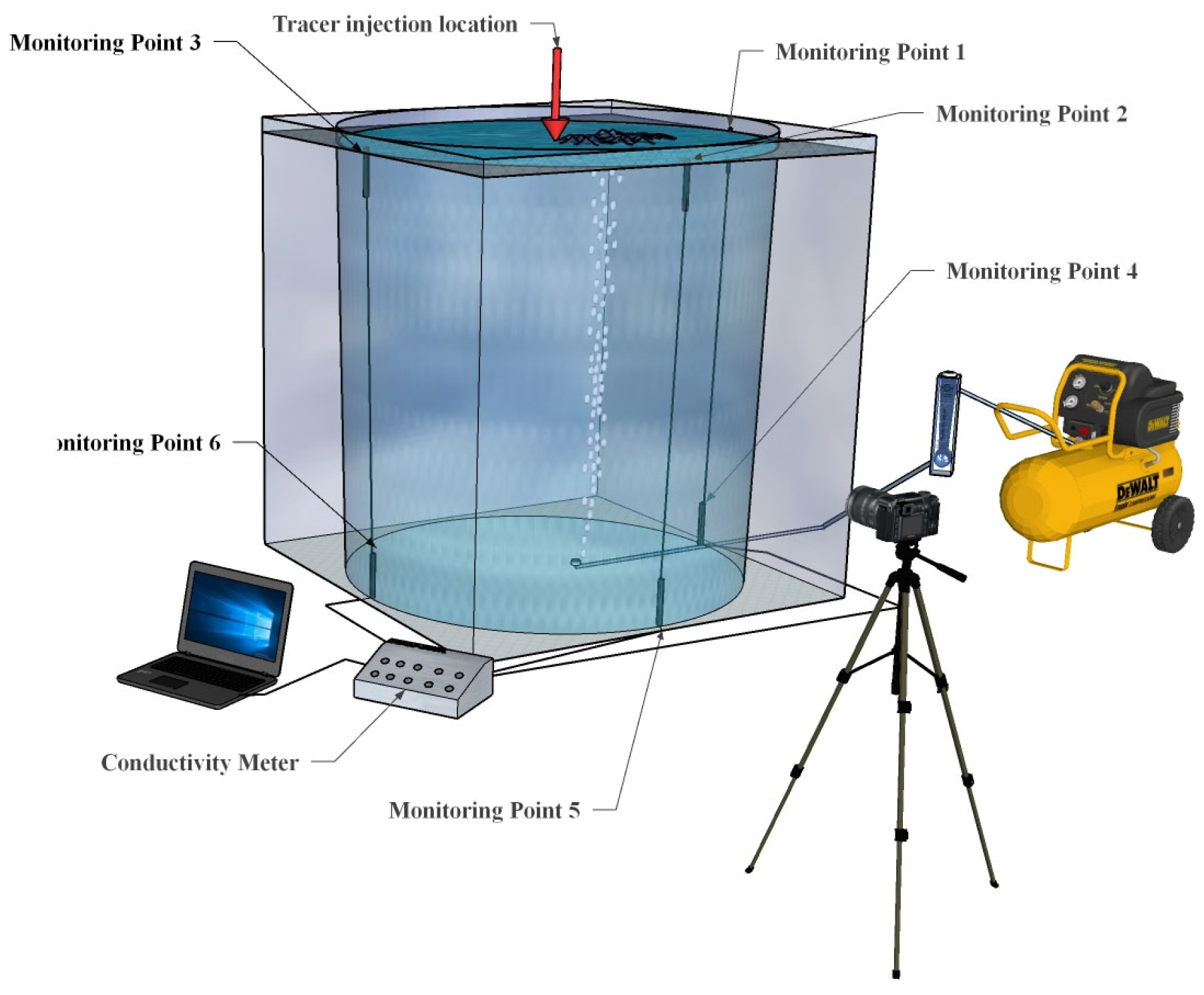
In the experiments, Platinum Black electrodes were employed as conductivity probes. Each probe had a volume of 0.118 cm³, and a total of six probes were installed, resulting in a combined volume of 0.708 cm³. Given that the total volume of the ladle model was 0.53 m³, the volume ratio of probes to the model was only 1.336 × 10⁻⁶. Therefore, the effect of probe volume on the flow behavior in the ladle water model can be considered negligible.

A saturated NaCl solution was used as the tracer, with a maximum injection volume of 695 mL, which accounted for 0.131% of the total water volume (530 L), corresponding to a mass fraction of 0.047%. At 20 °C, a 7% NaCl solution has a dynamic viscosity of 1.079 mPa·s compared to 1.005 mPa·s for pure water. Additionally, a 1% NaCl solution has a density of 1005 kg/m³, which is slightly higher than the density of water (998.2 kg/m³) [93]. Therefore, in the context of this study, the introduction of the tracer had a minimal effect on the viscosity and density of the fluid, and its impact on flow behavior was deemed insignificant. The water in the ladle was replaced after each experiment to maintain consistency.

To evaluate the repeatability of the experiment, a representative case involving the addition of 185 mL of saturated NaCl solution was selected for ten repeated trials. The resulting dimensionless concentration curves were compared and analyzed. As shown in Figure 2, the maximum and minimum concentration curves were used to generate a shaded region over time [90], visually representing the range of variation. These figures indicate that the variation range of the repeated experimental data at these monitoring points was relatively small compared to the average curve.

Table 4. Compare the mixing times of 10 trials and the average mixing time.

	1	2	3	4	5	6	7	8	9	10	AVG	S.D.
Monitoring Point 1	96.9	93.3	90.6	87.6	90.4	66.2	70.0	72.5	75.7	72.8	81.6	10.61
Monitoring Point 2	132.7	129.6	126.3	123.8	121.0	100.3	103.4	106.7	109.1	112.6	116.5	10.99
Monitoring Point 3	117.6	115.1	111.4	109.2	105.8	83.7	86.8	89.8	93.3	95.3	100.8	11.82
Monitoring Point 4	117.3	114.2	111.4	108.5	105.7	89.1	92.3	95.5	98.4	101.6	103.2	9.05
Monitoring Point 5	140.5	136.2	131.8	127.3	124.9	107.1	111.6	116.0	120.4	123.2	124	11.7
Monitoring Point 6	138.7	135.4	132.1	128.8	125.5	109.3	112.6	115.9	119.2	122.5	115.4	10.4

AVG: the average mixing time. S.D.: the standard deviation of the mixing time of ten trials.

summarizes the mixing times obtained from ten experimental repetitions. The average mixing time from the ten trials was adopted as the representative value for each monitoring point. The standard deviation between the individual mixing times and their average was also calculated. Results showed that the standard deviation at all monitoring points remained within 12%, indicating good repeatability and high reliability of the measured data.

In conclusion, the disturbance caused by the probe volume and tracer properties can be considered negligible. Furthermore, the dimensionless concentration curves and mixing time data demonstrated excellent repeatability. Thus, the experimental results were considered reliable and suitable for subsequent analysis.

3.2. Flow in Ladle Unit

The computational fluid dynamics (CFD) model results for the streamlines in the ladle are shown in Figure 3. In this study, the Euler–Euler multiphase flow model combined with the Realizable k-ε turbulence model was employed to solve the continuity and momentum equations, as well as to compute the steady-state flow field. The modeling strategy, mesh testing, simulation software (STAR-CCM+ 13.04), and validation followed the methodology used in our previous work [91]. Since these CFD results were not the primary focus of this study, a detailed simulation setup is not described here. From the simulation results, it can be observed that, after the gas entered through the bottom-blowing nozzle, a gas plume formed and rose toward the free surface. The flow field in the ladle can be divided into three regions: a large recirculating flow that forms on the left side of the ladle; a smaller recirculating flow that develops in the upper right region of the gas plume; and the left-side recirculating flow and the smaller right-side recirculating flow that meets in the lower-right region, merging into the gas plume, completing the circulation, and forming a fully developed flow field.

3.3. Transport Path of Tracer

Figure 4 illustrates the movement of a 100 mL ink–salt solution mixed tracer in the ladle under a bottom-blowing gas flow rate of 2.3 L/min after being injected at the center of the ladle’s liquid surface. At 1 s, the tracer penetrated the liquid surface and began convection transport downward. At 5 s, the tracer reached approximately one-third of the liquid depth (330 mm below the surface). By this time, the ink component had already spread across the surface, forming a black layer covering the entire top region. At 10 s, the ink started descending along the left-side wall, with significantly more ink observed on the left than on the right. At 15 s, the downward convection transport of the ink on both sides became nearly symmetrical. However, due to the gas injection port being located on the right side, the main recirculating flow occurred on the left, resulting in a higher ink concentration on the left side. Between 20 s and 30 s, the ink continued to convection transport downward at a synchronized and slow rate on both sides, indicating that, at 2.3 L/min, the gas flow had a significantly weaker influence on tracer movement compared to a higher gas flow rate of 8.3 L/min. At 35 s, the tracer began spreading from the bottom right toward the left, eventually dispersing throughout the ladle.

3.4. Tracer Transport Path and Analysis

Figure 5 presents the concentration–time curves at Monitoring Point 1 after adding tracer agents of different volumes into the water model of the ladle.

Table 5. The key points in the dimensionless concentration curves of Monitoring Point 1.

Tracer Volume (mL)	92	185	277	370	463	695
Response time (s)	8	8	5	8	8	9
Mixing time (s)	114	81.6	133.6	154.3	156.8	141.1

summarizes the key time points extracted from the dimensionless concentration curves. The tracer agent volumes were 92 mL, 185 mL, 277 mL, 370 mL, 463 mL, and 695 mL. All dimensionless concentration curves were obtained by averaging the results of ten experimental runs. After introducing 92 mL of saturated NaCl solution into the ladle, the dimensionless concentration at Monitoring Point 1 began to respond at 8 s, which was followed by a rapid increase. At 15 s, the concentration reached a peak value of 2.4, after which it rapidly decreased to 0.69 at 32 s, which represents the lowest concentration observed after the peak. Subsequently, the dimensionless concentration gradually rose and stabilized around 1. For the 185 mL tracer volume, the dimensionless concentration started to rise at 8 s and reached a maximum value of 3.37 at 18 s. Between 18 s and 36 s, the concentration decreased, reaching its lowest value of 0.75 at 36 s, after which it gradually increased and fluctuated around 1. When the tracer volume was 277 mL, the dimensionless concentration began to increase at 5 s, reaching its peak of 3.2 at 18 s. Subsequently, the concentration declined to 0.92, followed by a gradual rise after 35 s. A minor fluctuation was observed at 52 s, after which the curve stabilized around 1. For the 370 mL tracer volume, the dimensionless concentration started to rise after 8 s, reaching a peak value of 2.6 at 19 s. It then declined to 0.81, followed by a gradual increase after 43 s, and then eventually stabilizing within a ±5% standard range. After adding 463 mL of saturated NaCl solution, the concentration variation began at 8 s. The concentration continued to increase between 8 s and 19 s, reaching a peak of 2.76. From 19 s to 38 s, the concentration decreased to its lowest value of 0.75, then slowly rose and stabilized around 1. For the 695 mL tracer volume, the concentration started increasing at 9 s and reached a peak of 1.9 at 21 s. The concentration then declined to its lowest value of 0.64 at 39 s before gradually rising and stabilizing within the ±5% standard range. The initiation time of the concentration variation at Monitoring Point 1 remained around 8 s for all tracer volumes, indicating that changes in tracer volume do not significantly affect the response time at this location. However, the time required to reach the concentration peak varies with volume, recorded as 15 s, 18 s, 18 s, 19 s, 19 s, and 21 s for 92 mL, 185 mL, 277 mL, 370 mL, 463 mL, and 695 mL, respectively. This suggests that increasing the tracer volume delays the peak concentration occurrence. The peak concentration values for increasing tracer volumes were 2.4, 3.37, 3.2, 2.6, 2.76, and 1.9, respectively, indicating an initial increase followed by a decrease. The lower peak concentration at 92 mL was attributed to the small tracer volume, which, upon introduction, was largely carried by strong flow fields to the left side of the ladle, resulting in a lower tracer concentration on the right side. Consequently, the peak concentration at Monitoring Point 1 remained relatively low at 18 s. When the tracer volume exceeded 185 mL, a noticeable decline in peak concentration was observed. The duration from the concentration increase to peak occurrence for each tracer volume was recorded as 7 s, 10 s, 13 s, 11 s, 11 s, and 12 s, respectively, demonstrating that a larger tracer volume extended the time required to reach peak concentration. However, the duration of concentration declined following the peak, which was 17 s, 18 s, 17 s, 24 s, 19 s, and 18 s, respectively. Except for the 370 mL tracer volume, the time interval from peak-to-minimum concentration remained approximately 18 s for all cases, indicating that the tracer volume had minimal influence on the time span from peak-to-minimum concentration.

Figure 6 presents the concentration–time curves at Monitoring Point 2 after adding saturated NaCl solutions of different volumes into the ladle water model.

Table 6. The key points in the dimensionless concentration curves of Monitoring Point 2.

Tracer Volume (mL)	92	185	277	370	463	695
Response time (s)	8	8	9	10	9	9
Mixing time (s)	116.6	116.5	92.6	123	113	148.8

summarizes the key time points extracted from the dimensionless concentration curves. For a tracer volume of 92 mL, the dimensionless concentration began to change at 8 s and reached its peak value of 3.75 at 16 s. Between 16 s and 32 s, the concentration gradually decreased, reaching a minimum value of 0.67 at 32 s. Subsequently, a slight increase was observed, leading to a secondary peak at 51 s with a value of 1.4. When the tracer volume was 185 mL, the concentration started increasing at 8 s and reached a maximum of 2.2 at 18 s. Between 18 s and 33 s, the concentration rapidly decreased to its post-peak minimum of 0.44, after which it gradually stabilized around 1. For the 277 mL tracer volume, the dimensionless concentration began to rise at 9 s, reaching a peak of 2.2 at 19 s. The concentration then gradually decreased, reaching its lowest value of 0.56 at 34 s. After 34 s, the concentration gradually increased and stabilized within a ±5% standard range. When the tracer volume was 370 mL, the concentration response began at 10 s, reaching a peak value of 1.79 at 20 s. Subsequently, the concentration decreased, following a downward trend until reaching its minimum value of 0.45 at 37 s. Afterward, the concentration slowly rose and gradually stabilized around 1. For the 463 mL tracer volume, the conductivity sensor detected a response at 9 s, which was followed by a rapid increase in concentration between 9 s and 18 s. After reaching a maximum value of 2.1, the concentration began to decrease and reached its minimum of 0.51 at 36 s, subsequently stabilizing around 1. When the tracer volume reached 695 mL, the dimensionless concentration started rising at 9 s, reaching its peak of 1.35 at 20 s. It then underwent a sharp decline, reaching its minimum of 0.37 at 38 s, after which it gradually increased and stabilized around 1. For all six tracer volumes, the response time at Monitoring Point 2 was approximately 9 s, indicating that the tracer volume did not significantly affect the electrical conductivity response time at this location. As the tracer volume increased from 92 mL to 695 mL, the times required to reach peak concentration were 16 s, 18 s, 19 s, 20 s, 18 s, and 20 s, respectively. This suggests that a larger tracer volume delays the time to reach the maximum concentration, indicating an influence on the transport velocity of dissolved salts. The peak concentration values for increasing the tracer volumes were recorded as 3.75, 2.2, 2.2, 1.8, 2.1, and 1.35, respectively, demonstrating a general decreasing trend. This trend was attributed to the increased volume reducing the salt concentration at this point, as well as the excessive tracer volumes leading to salt settling at the bottom. By comparing the six dimensionless concentration curves under two different flow rates, it was observed that, at a flow rate of 2.3 L/min, secondary peaks were rarely present, and this phenomenon became even less frequent as the tracer volume increased. This was due to the lower flow rate limiting the movement of dissolved salts along the ladle’s flow field, preventing a substantial amount of salts from re-accumulating and reaching the upper monitoring point, which would otherwise result in a secondary peak. Additionally, the minimum concentration values at 2.3 L/min were consistently lower than those observed at 8.3 L/min. This is because the lower flow rate failed to keep salts suspended in the upper region, which caused them to settle due to buoyancy force, leading to lower minimum values at the upper monitoring point. Furthermore, the recovery from the minimum concentration to the ±5% standard level predominantly exhibited a slow growth trend.

Figure 7 presents the concentration–time curves at Monitoring Point 3 after adding tracer agents of six different volumes into the ladle water model.

Table 7. The key points in the dimensionless concentration curves of Monitoring Point 3.

Tracer Volume (mL)	92	185	277	370	463	695
Response time (s)	8	10	8	10	8	9
Mixing time (s)	129.6	100.8	102.9	125.5	126.1	143

summarizes the key time points extracted from the dimensionless concentration curves. For a tracer volume of 92 mL, the dimensionless concentration began to rise at 8 s and reached its maximum value of 8 at 15 s. The concentration increased rapidly, with a steep slope observed in the concentration curve between 8 s and 15 s. In the interval from 15 s to 40 s, the concentration exhibited a rapid downward trend, indicating that a large amount of dissolved salt quickly passed through this location. At 50 s, a secondary peak appeared with a value of 1.52, which was followed by a gradual decrease until the concentration stabilized at 1. When the tracer volume was 185 mL, the concentration started increasing at 10 s and reached a maximum value of 3.4 at 21 s. Subsequently, the concentration declined until it stabilized at 1. For the 277 mL tracer volume, the electrical conductivity response was still detected at 8 s, with the concentration reaching a peak value of 2.7 at 19 s. The concentration then continued to decrease until 50 s, reaching a value of 0.76, after which it gradually rose and stabilized at 1. When 370 mL of saturated NaCl solution was introduced, the concentration began to increase slowly at 10 s, which was followed by a rapid rise after 15 s, reaching a peak value of 1.6 at 23 s. Thereafter, the concentration followed a general downward trend, reaching its lowest value of 0.66 at 55 s. After 55 s, the concentration gradually increased until complete mixing was achieved. For the 463 mL tracer volume, the concentration started rising at 8 s, reaching a peak of 2.6 at 20 s. The overall trend of the concentration curve was similar to that observed for the 370 mL tracer volume. When the tracer volume was 695 mL, the concentration increased from 9 s, reaching its peak value of 1.9 at 20 s. From 20 s to 46 s, the concentration followed a decreasing trend, reaching a minimum value of 0.59 at 46 s, after which it slowly increased and eventually stabilized within a ±5% standard range. The response time at Monitoring Point 3 remained around 8 s, indicating that the upper monitoring point’s response time was not significantly affected by the tracer volume. However, at a flow rate of 8.3 L/min, the response time at the upper monitoring point varied noticeably with tracer volume, suggesting a clear relationship between the gas injection rate and the time required for the tracer to reach the upper monitoring point. Since the response times at the three upper monitoring points were similar (all around 8 s), it can be concluded that the gas injection nozzle had little effect on the liquid velocity near the free surface. By comparing the six dimensionless concentration curves in Figure 7, it was observed that the first peak value generally decreased with increasing tracer volume. This phenomenon occurred because, at smaller tracer volumes, nearly all of the tracer followed the strong recirculating flow to Monitoring Point 3. As the tracer volume increased, the added tracer initially moved downward, temporarily disrupting the flow field in the ladle water model, leading to partial salt deposition. Once the flow field stabilized, only a small amount of salt was transported to the upper Monitoring Point 3 by recirculating flow, resulting in a lower first peak as the tracer volume increased. Furthermore, at Monitoring Point 3, the first peak values under a lower flow rate (2.3 L/min) were consistently lower than those observed at a higher flow rate (8.3 L/min), further confirming that variations in gas flow rate significantly influence the transport behavior of the tracer within the ladle.

Figure 8 presents the concentration–time curves at Monitoring Point 4 after introducing tracer agents of different volumes into the ladle.

Table 8. The key points in the dimensionless concentration curves of Monitoring Point 4.

Tracer Volume (mL)	92	185	277	370	463	695
Response time (s)	24	23	18	13	14	13
Mixing time (s)	123.6	103.2	130.8	147.3	151.2	168.8

summarizes the key time points extracted from the dimensionless concentration curves. When 92 mL of saturated NaCl solution was added, two distinct concentration trends, Trend 1 and Trend 2, were observed in the dimensionless concentration curve at Monitoring Point 4. The black curve in the figure represents the average of both trends. The primary difference between these trends lay in their initial concentration behavior: Trend 1 exhibited a gradual increase from zero without pronounced peaks before reaching a dimensionless concentration of 1, whereas Trend 2 showed a rapid increase in concentration with noticeable but relatively small peaks immediately after the response began. A similar phenomenon was observed when the tracer volume increased to 185 mL, with the concentration curve displaying both trends similar to those observed for the 92 mL tracer. This behavior was mainly attributed to the small tracer volume being more significantly affected by the recirculating flow within the ladle, making it highly sensitive to minor variations in the flow field. Consequently, subtle changes in the ladle’s flow conditions altered the tracer transport direction, leading to the emergence of two distinct trends [90,91]. Trend 1 closely resembled the previously studied Path 2 curve, indicating that, after injection, the tracer was primarily transported through the left and central regions of the ladle before gradually crossing the gas plume and reaching Monitoring Point 4. In contrast, Trend 2 was similar to the Path 5 curve, suggesting that the tracer predominantly circulated on the right side, leading to the appearance of peak values in the concentration curve. When the tracer volume increased to 277 mL, the dimensionless concentration began to change at 18 s and reached its peak of 1.92 at 40 s. A minor trough appeared at 52 s, with the concentration dropping to 1.36. Between 52 s and 57 s, the concentration increased again, reaching 1.7, before gradually declining after 57 s, until then stabilizing within the range of 0.95–1.05. For a tracer volume of 370 mL, the concentration response began at 13 s, which was followed by a rapid increase, reaching a maximum of 5.4 at 32 s. Subsequently, the concentration declined sharply, reaching its lowest value of 1.39 at 86 s. A temporary increase was observed between 86 s and 103 s, leading to a second peak at 103 s with a value of 1.82. Afterward, the concentration continuously decreased until it stabilized around 1. When 463 mL of saturated NaCl solution was introduced, the concentration started increasing at 14 s, showing a rapid growth phase until 22 s, after which the growth rate slowed. The concentration reached a maximum of 2.27 at 47 s, which was followed by a continuous decline. By 72 s, the concentration decreased to 1.2. Between 72 s and 104 s, fluctuations were observed, with a secondary peak appearing at 104 s with a value of 1.5. Afterward, the concentration gradually decreased with minor oscillations until stabilizing within the required range. For the 695 mL tracer volume, the concentration began to respond at 13 s, which was followed by a rapid increase, reaching a peak of 3.7 at 37 s. After 37 s, the concentration continuously declined with significant fluctuations until complete mixing was achieved. The initial response time of the dimensionless concentration curve for tracer volumes of 92 mL and 185 mL was 24 s and 23 s. For tracer volumes of 277 mL, 370 mL, 463 mL, and 695 mL, the initial response times were 18 s, 13 s, 14 s, and 13 s, respectively. This suggests that, when the tracer volume was small, its transport path was significantly influenced by the flow field, leading to a delayed response at Monitoring Point 4. However, as the tracer volume increased, the influence of the flow field on transport pathways decreased, resulting in a more consistent response time at Monitoring Point 4. Furthermore, with increasing tracer volume, Trend 2 became dominant in the concentration curves at Monitoring Point 4.

Figure 9 presents the concentration–time curves at Monitoring Point 5 after adding tracer agents of different volumes into the ladle.

Table 9. The key points in the dimensionless concentration curves of Monitoring Point 5.

Tracer Volume (mL)	92	185	277	370	463	695
Response time (s)	25	20	20	15	22	15
Mixing time (s)	141	124	134.4	136.1	142.7	191.2

summarizes the key time points extracted from the dimensionless concentration curves. For a tracer volume of 92 mL, the concentration curve began to change at 25 s. Before complete mixing was achieved, the concentration remained below 1, indicating that the dimensionless concentration increased gradually from zero to 1 with minor fluctuations. A relatively faster increase was observed only between 15 s and 25 s. When the tracer volume was 185 mL, the dimensionless concentration started changing at 20 s. However, between 20 s and 27 s, the concentration increased very slowly, indicating that the tracer reached this location at approximately 27 s. Between 27 s and 39 s, the concentration increased rapidly. After 39 s, noticeable fluctuations appear in the concentration curve, which was followed by a gradual decrease until mixing was complete. For the 277 mL tracer volume, the concentration began to change at 20 s. Similar to the 185 mL case, the concentration exhibited minimal variation between 20 s and 28 s, suggesting that only a small amount of salt reached this location initially. Between 28 s and 43 s, the concentration increased rapidly, reaching a maximum value of 1.38 at 49 s. The concentration then declined from 49 s to 61 s, briefly reaching a local minimum of 1.1, which was followed by a slight increase to 1.3. After 69 s, the concentration decreased with minor fluctuations until stabilizing within the range of 0.95–1.05. When the tracer volume increased to 370 mL, the concentration response began at 15 s, which was followed by a rapid increase, reaching 4 at 30 s. Subsequently, the concentration gradually declined, exhibiting significant fluctuations that resulted in a jagged pattern of peaks. Eventually, the concentration stabilized around 1. For the 463 mL tracer volume, the concentration starts increasing at 22 s, with multiple peaks appearing in the curve. The highest peak, reaching 1.9, occurred at 59 s. However, due to significant fluctuations, a clear trend was not observed. When the tracer volume reached 695 mL, the concentration began changing at 15 s, followed by a rapid increase, reaching 3.2 at 26 s. After a brief fluctuation, the concentration continued to rise, reaching a maximum value of 3.7 at 39 s. Beyond 39 s, the concentration exhibited an overall decreasing trend but was accompanied by significant fluctuations, resulting in a jagged concentration curve. These oscillations persisted until approximately 150 s before stabilizing. The response times for different tracer volumes at Monitoring Point 5 were recorded as 25 s, 20–27 s, 20–28 s, 15 s, 22 s, and 15 s, respectively. Most of the response times fell within the 20–25 s range, with the remaining cases occurring at 15 s. This suggests that the first arrival time of the tracer at Monitoring Point 5 was not uniform, indicating the possibility of multiple transport pathways leading to that location. Additionally, the maximum concentrations recorded for different tracer volumes were 1, 1.13, 1.38, 4, 1.9, and 3.7, respectively. The significant variation in both peak concentration values and their occurrence times further confirmed that the tracer reached this point via multiple, possibly non-unique transport pathways.

Figure 10 presents the concentration–time curves at Monitoring Point 6 after introducing saturated NaCl solutions of different volumes (92 mL, 185 mL, 277 mL, 370 mL, 463 mL, and 695 mL) into the ladle water model.

Table 10. The key points in the dimensionless concentration curves of Monitoring Point 6.

Tracer Volume (mL)	92	185	277	370	463	695
Response time (s)	25	23	25	18	20	17
Mixing time (s)	141.5	115.4	144	162.5	170	198.3

summarizes the key time points extracted from the dimensionless concentration curves. For a 92 mL tracer volume, the dimensionless concentration curve began to change at 25 s. However, between 25 s and 35 s, the concentration remained relatively stable, showing no significant increase. After 35 s, a rapid rise was observed, reaching 1.0 at 58 s. From 58 s to 68 s, the concentration decreased to 0.83, which was followed by a gradual increase until it fluctuated around 1.0. When the 185 mL tracer was added, the concentration began to rise at 23 s, showing rapid growth and reaching a maximum of 1.35 at 53 s. After a slight decrease, the concentration increased again to 1.34 at 71 s, which was followed by a gradual decline until complete mixing was achieved. For the 277 mL tracer volume, the concentration started changing at 25 s. Between 25 s and 35 s, the concentration increased rapidly. After 35 s, the concentration curve exhibited a sawtooth pattern, which is characterized by fluctuations with relatively small variations in overall concentration. The peak concentration of 1.37 was recorded at 85 s. When the 370 mL tracer volume was introduced, the concentration began increasing at 18 s, showing a very rapid growth phase. At 35 s, the concentration momentarily stabilized before experiencing a slight decrease, reaching 3.3 at 46 s. The concentration then increased again to 4.5 at 50 s, which was followed by a general downward trend. Throughout the decline, significant fluctuations were observed until the concentration eventually stabilized near 1.0. For the 463 mL tracer volume, the conductivity sensor detected a response at 20 s, which was followed by a rapid increase between 20 s and 40 s. The concentration reached a peak value of 2.6 at 40 s, after which it gradually decreased until complete mixing was achieved. Minor fluctuations were observed throughout the decline. When the 695 mL tracer was added, the concentration started changing at 17 s and exhibited a very rapid increase, reaching 3.7 at 31 s. A short-lived decrease followed, with the concentration dropping to 2.5 at 55 s. After 55 s, the concentration increased slightly again, peaking at 2.9 at 61 s. Subsequently, the concentration followed a general downward trend, which was accompanied by fluctuations. The dimensionless concentration curve at Monitoring Point 6 showed significant fluctuations, with multiple secondary peaks and sawtooth-like oscillations during the concentration decline. This suggests that the tracer, after reaching this location, accumulated and settled before being gradually transported away in batches under the influence of the gas plume, rather than being immediately and entirely dispersed. This stepwise removal process resulted in the observed oscillatory behavior. The sensor response times for different tracer volumes were recorded as 25 s, 23 s, 25 s, 18 s, 20 s, and 17 s, respectively. As the tracer volume increased, the response time of the conductivity sensor gradually shortened, indicating that larger tracer volumes were transported to Monitoring Point 6 more quickly under the influence of the gas plume. Additionally, as the tracer volume increased, sedimentation at Monitoring Point 6 became more pronounced, leading to a prolonged mixing time at this location.

3.5. Analysis of Mixing Time

Figure 11 illustrates the mixing times at various monitoring points after introducing tracer agents of different volumes into the ladle water model. At Monitoring Point 1, the mixing times corresponding to tracer volumes of 92 mL, 185 mL, 277 mL, 370 mL, 463 mL, and 695 mL were 114 s, 81.6 s, 133.6 s, 154.3 s, 156.8 s, and 141.1 s, respectively. The mixing time initially decreased, which was followed by an increase and then another decrease. Two transition points were identified at 185 mL and 463 mL, where the mixing time significantly decreased when the tracer volume increased from 92 mL to 185 mL, which was followed by a continuous increase from 185 mL to 463 mL. However, when the volume increased to 695 mL, the mixing time shortened again. At Monitoring Point 2, the mixing times for increasing tracer volumes were 116.6 s, 116.5 s, 92.6 s, 123 s, 113 s, and 148.8 s, respectively. The mixing time exhibited two increasing phases, occurring between 277 mL to 370 mL and 463 mL to 695 mL. For Monitoring Point 3, the mixing times corresponding to 92 mL, 185 mL, 277 mL, 370 mL, 463 mL, and 695 mL were 129.6 s, 100.8 s, 102.9 s, 125.5 s, 126.1 s, and 143 s, respectively. The mixing time first decreased, then increased, and then remained in an upward trend when the tracer volume exceeded 185 mL. At Monitoring Point 4, the mixing times for increasing tracer volumes were 123.6 s, 103.2 s, 130.8 s, 147.3 s, 151.2 s, and 168.8 s. Notably, when the tracer volume was 185 mL, the mixing time was significantly shorter than for other tracer volumes. For Monitoring Point 5, the mixing times corresponding to different tracer volumes were 141 s, 124 s, 134.4 s, 136.1 s, 142.7 s, and 191.2 s, respectively. A trend of initial reduction followed by an increase was observed. At Monitoring Point 6, the mixing times for increasing tracer volumes were 141.5 s, 115.4 s, 144 s, 162.5 s, 170 s, and 198.3 s. Similar to other locations, the mixing time first decreased and then increased, with the longest mixing time observed at 695 mL, making it the longest among all six monitoring points. As the tracer volume changed, the mixing time at all six monitoring points also varied accordingly, generally exhibiting a trend of initial shortening followed by an increase. Figure 11 also shows that the mixing times at the bottom monitoring points were relatively concentrated, following similar trends, with a high degree of overlap among different tracer volumes. In contrast, the mixing time variations at the upper monitoring points were less consistent, suggesting that the upper regions were more susceptible to changes in tracer volume.

Figure 12 shows that the mixing times at the upper monitoring points were generally shorter than those at the lower monitoring points. This difference was particularly pronounced when larger tracer volumes were introduced as the mixing times at the lower monitoring points became significantly longer than those at the upper monitoring points. This observation suggests that the gas flow rate was insufficient to fully disperse larger volumes of tracer within the ladle. The three-dimensional visualization further confirmed that when the tracer volume was 185 mL, the mixing time was notably shorter compared to other tracer volumes. Additionally, the mixing time initially decreased and then increased as the tracer volume increased.

3.6. Analysis of Tracer Concentration Experiments

To further clarify the relative influence of the tracer volume and concentration on mixing behavior, a set of controlled experiments was designed in which the tracer volume was held constant at 185 mL, thereby keeping the total liquid volume in the system unchanged. The effect of different NaCl mass concentrations on the mixing process was evaluated by varying the NaCl concentration while maintaining a constant volume. The selected concentrations were 6.63%, 13.25%, 19.68%, and 26.5%.

As shown in Figure 13a–c, changes in NaCl concentration had a limited impact on the dimensionless concentration curves at the upper monitoring points. The tracer arrival time at the top was nearly identical across all concentrations, and the differences in the time to initial response were minimal. This indicates that the tracer response in the upper region was relatively stable. However, the peak concentration decreased progressively as the NaCl concentration decreased, suggesting that, although the diffusion rate was not significantly affected, the signal intensity detected by the probes was influenced by the tracer concentration. In contrast, as shown in Figure 13d–f, the effect of the NaCl concentration was more pronounced at the bottom monitoring points. Notably, when the NaCl concentration was 19.68%, the bottom monitoring points exhibited significantly higher peak values than those observed under the other three conditions. This indicates that, at this concentration, the transport and accumulation of the tracer in the lower region was more effective. Moreover, at higher concentrations (19.68% and 26.5%), larger differences between the concentration curves were observed, whereas, at lower concentrations (6.63% and 13.25%), the curves tended to converge, indicating reduced sensitivity to concentration changes. Further analysis from Figure 14 reveals that the influence of NaCl concentration on the mixing time varied among different monitoring points. The most significant effects were observed at Monitoring Points 3, 4, and 6. Nevertheless, the overall mixing trends remained consistent, indicating that, while concentration changes can affect local signal intensity and mixing time, they do not significantly alter the global mixing behavior. In summary, the results of the controlled concentration experiments suggest that, under a constant tracer volume, the effect of the NaCl concentration on mixing behavior is region-specific, with the bottom of the ladle being more sensitive to concentration variations.

4. Conclusions

A water model with a geometric similarity ratio of 1:3 based on the 130 t steel ladle of the steel plant was established to study the transmission path and mixing time of the tracer under low flow conditions, and the following conclusions were made:

• At a bottom-blowing gas flow rate of 2.3 L/min, two distinct trends appeared in the dimensionless concentration curve at Monitoring Point 4 when the tracer volume was 92 mL or 185 mL. This indicates that, at low tracer volumes, the tracer transport path to Monitoring Point 4 was unstable due to the significant influence of the gas plume. As the tracer volume increased, only one dominant transport path was observed. When the bottom-blowing gas flow rate was 8.3 L/min, only two trends were observed at a tracer volume of 92 mL.
• When the tracer volume was too small, the dimensionless concentration curve at Monitoring Point 4 exhibited either a sinusoidal or parabolic shape. If the tracer first moved through the left-side and central regions before slowly crossing the gas plume to reach Monitoring Point 4, the curve followed a parabolic shape. If the tracer predominantly circulated on the right side, the curve exhibited a sinusoidal pattern. When the tracer volume exceeded 277 mL, the concentration curve at Monitoring Point 4 was always sinusoidal.
• Regardless of the gas flow rate, Monitoring Point 3 exhibited the highest peak concentration among the six monitoring points. At a bottom-blowing gas flow rate of 8.3 L/min, the peak concentration at Monitoring Point 3 was significantly higher than that observed at 2.3 L/min.
• Different bottom-blowing gas flow rates led to distinct trends in the mixing time variation with increasing tracer volume. At 2.3 L/min, the mixing time at the bottom first decreased and then increased, reaching the shortest duration at 185 mL. At 8.3 L/min, the mixing time at the bottom monitoring points decreased continuously with increasing tracer volume, whereas, at the top monitoring points, the mixing time first decreased and then increased.
• At different bottom-blowing gas flow rates, the mixing time at the upper monitoring points was consistently shorter than at the lower monitoring points.
• At a bottom-blowing gas flow rate of 2.3 L/min, the optimal tracer volume range was 185 mL–277 mL. This ensured a stable transport path while minimizing the flow field disturbances caused by tracer injection.
• The tracer concentration experiments indicate that variations in concentration have a considerable impact on the mixing behavior at the bottom of the ladle, while their influence on the overall mixing trend remains limited. When the tracer concentration is relatively low, the mixing behavior throughout the ladle becomes more uniform.

References

1. Szekely, J.; Carlsson, G.; Helle, L. Ladle Metallurgy; Springer: Berlin/Heidelberg, Germany, 1989; pp. 27–71. [Google Scholar]
2. Mazumdar, D.; Guthrie, R.L. The Physical and mathematical modelling of gas stirred ladle systems. ISIJ Int. 1995, 35, 1–20. [Google Scholar] [CrossRef]
3. Jönsson, P.; Jonsson, L.I. The Use of Fundamental Process Models in Studying Ladle Refining Operations. ISIJ Int. 2001, 41, 1289–1302. [Google Scholar] [CrossRef]
4. Mazumdar, D.; Evans, J.W. Macroscopic Models for Gas Stirred Ladles. ISIJ Int. 2004, 44, 447–461. [Google Scholar] [CrossRef]
5. Xin, Z.; Zhang, J.; Peng, K.; Zhang, J.; Zhang, C.; Liu, Q. Modeling of LF refining process: A review. J. Iron Steel Res. Int. 2024, 31, 289–317. [Google Scholar] [CrossRef]
6. Niu, K.J.; Feng, W.H.; Conejo, A.N.; Ramírez-Argáez, M.A.; Yan, H. 3D CFD Model of Ladle Heat Transfer with Gas Injection. Metall. Mater. Trans. B 2023, 54, 2066–2079. [Google Scholar] [CrossRef]
7. Conejo, A.N. Physical and Mathematical Modelling of Mass Transfer in Ladles due to Bottom Gas Stirring: A Review. Processes 2020, 8, 750. [Google Scholar] [CrossRef]
8. Niu, K.J.; Feng, W.H.; Conejo, A.N. Effect of the Nozzle Radial Position and Gas Flow Rate on Mass Transfer during Bottom Gas Injection in Ladles with One Nozzle. Metall. Mater. Trans. B 2022, 53, 1344–1350. [Google Scholar] [CrossRef]
9. Yang, R.; Chen, C.; Lin, Y.; Zhao, Y.; Zhao, J.; Zhu, J.; Yang, S. Water model experiment on motion and melting of scarp in gas stirred reactors. Chin. J. Process Eng. 2022, 22, 954–962. [Google Scholar] [CrossRef]
10. Ji, S.; Niu, K.J.; Conejo, A.N. Multiphase modeling of steel-slag mass transfer through distorted interface in bottom-stirred ladle. ISIJ Int. 2024, 64, 52–58. [Google Scholar] [CrossRef]
11. Podder, A.; Coley, K.S.; Phillion, A.B. Modeling Study of Steel–Slag–Inclusion Reactions During the Refining of Si–Mn Killed Steel. Steel Res. Int. 2022, 93, 2100831. [Google Scholar] [CrossRef]
12. Podder, A.; Coley, K.S.; Phillion, A.B. Simulation of Ladle Refining Reactions in Si–Mn-Killed Steel. Steel Res. Int. 2024, 95, 2300330. [Google Scholar] [CrossRef]
13. Duan, H.J.; Zhang, L.F.; Thomas, B.G.; Conejo, A.N. Fluid Flow, Dissolution, and Mixing Phenomena in Argon-Stirred Steel Ladles. Metall. Mater. Trans. B 2018, 49, 2722–2743. [Google Scholar] [CrossRef]
14. Li, X.L.; Wang, H.H.; Tian, J.; Wang, D.Y.; Qu, T.P.; Hou, D.; Hu, S.Y.; Wu, G.J. Investigation on the Alloy Mixing and Inclusion Removement through Using a New Slot-Porous Matched Tuyeres. Metals 2023, 13, 667. [Google Scholar] [CrossRef]
15. Wen, X.; Ren, Y.; Zhang, L.F. Effect of CaF2 Contents in Slag on Inclusion Absorption in a Bearing Steel. Steel Res. Int. 2022, 94, 2200218. [Google Scholar] [CrossRef]
16. Kim, T.S.; Yang, J.; Park, J.H. Effect of Physicochemical Properties of Slag on the Removal Rate of Alumina Inclusions in the Ruhrstahl–Heraeus (RH) Refining Conditions. Metall. Mater. Trans. B 2022, 53, 2523–2533. [Google Scholar] [CrossRef]
17. Conejo, A.N.; Kitamura, S.; Maruoka, N.; Kim, S.J. Effects of Top Layer, Nozzle Arrangement, and Gas Flow Rate on Mixing Time in Agitated Ladles by Bottom Gas Injection. Metall. Mater. Trans. B 2013, 44, 914–923. [Google Scholar] [CrossRef]
18. Terrazas, M.S.C.; Conejo, A.N. Effect of Nozzle Diameter on Mixing Time During Bottom-Gas Injection in Metallurgical Ladles. Metall. Mater. Trans. B 2014, 45, 711–718. [Google Scholar] [CrossRef]
19. Feng, W.H.; Conejo, A.N. Physical and Numerical Simulation of the Optimum Nozzle Radial Position in Ladles with One Nozzle and Bottom Gas Injection. ISIJ Int. 2022, 62, 1211–1221. [Google Scholar] [CrossRef]
20. Conejo, A.N.; Feng, W.H. Ladle Eye Formation Due to Bottom Gas Injection: A Reassessment of Experimental Data. Metall. Mater. Trans. B 2022, 53, 999–1017. [Google Scholar] [CrossRef]
21. Wondrak, T.; Timmel, K.; Bruch, C.; Gardin, P.; Hackl, G.; Lachmund, H.; Lüngen, H.B.; Odenthal, H.J.; Eckert, S. Large-Scale Test Facility for Modeling Bubble Behavior and Liquid Metal Two-Phase Flows in a Steel Ladle. Metall. Mater. Trans. B 2022, 53, 1703–1720. [Google Scholar] [CrossRef]
22. Wang, R.D.; Jin, Y.; Cui, H. The Flow Behavior of Molten Steel in an RH Degasser Under Different Ladle Bottom Stirring Processes. Metall. Mater. Trans. B 2022, 53, 342–351. [Google Scholar] [CrossRef]
23. Jojo-Cunningham, Y.; Guo, X.P.; Zhou, C.; Liu, Y. Volumetric Flow Field inside a Gas Stirred Cylindrical Water Tank. Fluids 2024, 9, 11. [Google Scholar] [CrossRef]
24. Chen, C.; Cheng, G.G.; Yang, H.K.; Hou, Z.B. Physical Modeling of Fluid Flow Characteristics in a Delta Shaped, Four-Strand Continuous Casting Tundish with Different Flow Control Devices. Adv. Mater. Res. 2011, 284, 1071–1079. [Google Scholar] [CrossRef]
25. Schwarz, M.P.; Koh, P.T.L. Numerical Modelling of Bath Mixing by Swirled Gas Injection. In Proceedings of the SCANINJECT IV-4th International Conference on Injection Metallurgy, Luleå, Sweden, 11–13 July 1986. [Google Scholar]
26. Schwarz, M.P.; Turner, W.J. Applicability of the standard k-ϵ turbulence model to gas-stirred baths. Appl. Math. Model. 1988, 12, 273–279. [Google Scholar] [CrossRef]
27. Zhao, J.X.; Zhu, H.Y.; Chen, J.; Wang, L.Q.; Yan, X.B.; Sun, J. Numerical Simulation on the Motion Behavior of Micro-Inclusions at the Steel-Slag Interface. Metall. Mater. Trans. B 2024, 55, 1700–1711. [Google Scholar] [CrossRef]
28. Zhong, J.; Xu, J.; Luo, D.Q.; Liu, S.D.; Zhou, Z.Y.; Lai, C.B. Numerical Simulation on Dehydrogenation Behavior During Argon Blowing Enhanced Vacuum Refining Process of High-Quality Steel. J. Mater. Res. Technol. 2024, 33, 6481–6493. [Google Scholar] [CrossRef]
29. Nick, R.S.; Teng, L.; Yang, H.L.; Tilliander, A.; Glaser, B.; Sheng, D.Y.; Jönsson, P.G.; Björkvall, J. Mathematical modelling of novel combined stirring method during the final stage of ladle refining. Ironmak. Steelmak. 2023, 50, 721–733. [Google Scholar] [CrossRef]
30. Wang, J.H.; Ni, P.Y.; Chen, C.; Ersson, M.; Li, Y. Effect of gas blowing nozzle angle on multiphase flow and mass transfer during RH refining process. Int. J. Miner. Metall. Mater. 2023, 30, 844–856. [Google Scholar] [CrossRef]
31. Li, X.L.; Wang, D.Y.; Tian, J.; Wang, H.H.; Qu, T.P.; Hou, D.; Hu, S.Y.; Zhang, Z.X.; Zhou, X.Z.; Wu, G.J. Modeling of Bubble Transportation, Expansion, as Well as Adhesion of Inclusions in a Ladle with Different Tuyeres. Metall. Mater. Trans. B 2024, 55, 14–31. [Google Scholar] [CrossRef]
32. Zhou, X.B.; Zhang, Y.; He, Q.L.; Ni, P.Y.; Yue, Q.; Ersson, M. Novel Evaluation Method to Determine the Mixing Time in a Ladle Refining Process. Metall. Mater. Trans. B 2022, 53, 4114–4123. [Google Scholar] [CrossRef]
33. Hua, C.J.; Bao, Y.P.; Wang, M. Multiphysics numerical simulation model and hydraulic model experiments in the argon-stirred ladle. Processes 2022, 10, 1563. [Google Scholar] [CrossRef]
34. Tiwari, R.; Girard, B.; Labrecque, C.; Isac, M.M.; Guthrie, R.I.L. CFD Predictions for Mixing Times in an Elliptical Ladle Using Single- and Dual-Plug Configurations. Processes 2023, 11, 1665. [Google Scholar] [CrossRef]
35. Schwarz, M.P. Buoyancy and expansion power in gas-agitated baths. ISIJ Int. 1991, 31, 947–951. [Google Scholar] [CrossRef]
36. Schwarz, M.P.; Dang, P. Simulation of Blowthrough in Smelting Baths with Bottom Gas Injection. In Proceedings of the 13th Process Technology Conference Proceedings, Nashville, TN, USA, 2–5 April 1995; pp. 415–421. [Google Scholar]
37. Ramírez-López, A. Analysis of Mixing Efficiency in a Stirred Reactor Using Computational Fluid Dynamics. Symmetry 2024, 16, 237. [Google Scholar] [CrossRef]
38. Ramírez-López, A. Analysis of the Hydrodynamics Behavior Inside a Stirred Reactor for Lead Recycling. Fluids 2023, 8, 268. [Google Scholar] [CrossRef]
39. Li, X.L.; Hu, S.Y.; Wang, D.Y.; Qu, T.P.; Wu, G.J.; Zhang, P.; Quan, Q.; Zhou, X.Z.; Zhang, Z.X. Inclusion Removements in a Bottom-Stirring Ladle with Novel Slot-Porous Matched Dual Plugs. Metals 2022, 12, 162. [Google Scholar] [CrossRef]
40. Sun, Y.P.; Duan, H.J.; Zhang, L.F. A Boundary Layer Model for Capture of Inclusions by Steel-Slag Interface in a Turbulent Flow. J. Iron Steel Res. Int. 2023, 30, 1101–1108. [Google Scholar] [CrossRef]
41. Huang, C.; Duan, H.J.; Zhang, L.F. Modeling of Motion of Inclusions in Argon-Stirred Steel Ladles. Steel Res. Int. 2024, 95, 2300537. [Google Scholar] [CrossRef]
42. Cao, J.Q.; Li, Y.; Lin, W.M.; Che, J.L.; Zhou, F.; Tan, Y.F.; Li, D.L.; Dang, J.; Chen, C. Assessment of Inclusion Removal Ability in Refining Slags Containing Ce2O3. Crystals 2023, 13, 202. [Google Scholar] [CrossRef]
43. Wei, T.X.; Oeters, F. A model test for emulsion in gas-stirred ladles. Steel Res. 1992, 63, 60–68. [Google Scholar] [CrossRef]
44. Lou, W.; Zhu, M. Numerical simulations of inclusion behavior and mixing phenomena in gas-stirred ladles with different arrangment of tuyeres. ISIJ Int. 2014, 54, 9–18. [Google Scholar] [CrossRef]
45. Villarreal-Medina, R.; Jardón–pérez, L.E.; Amaro–Villeda, A.M.; Trápaga–Martínez, G.; Ramírez–Argáez, M.A. Effect of the Injection Position on Mixing Time in a Centric Gas-stirred Ladle Water Model Assisted by a Systematic CFD Study. ISIJ Int. 2024, 64, 2079–2083. [Google Scholar] [CrossRef]
46. Xue, L.Q.; Zhao, Y.S.; Wang, J.; Wang, H.; Miao, Z.; Xiong, R.X.; Xu, Z.B.; Lin, W.M.; Niu, X.F.; Chen, C. The Flow Performance of Combined Gas Blowing at the Vacuum Chamber and Up-Snorkel in the Ruhrstahl–Heraeus (RH) Degasser for Electrical Steel Production. Processes 2025, 13, 448. [Google Scholar] [CrossRef]
47. Krishna-Murthy, G.G.; Elliott, J.F. Definition and Determination of Mixing Time in Gas Agitated Liquid Baths. ISIJ Int. 1992, 32, 190–195. [Google Scholar] [CrossRef]
48. Joo, S.; Guthrie, R.I.L. Modeling flows and mixing in steelmaking ladles designed for single- and dual-plug bubbling operations. Metall. Mater. Trans. B 1992, 23, 765–778. [Google Scholar] [CrossRef]
49. Zhu, M.Y.; Inomoto, T.; Sawada, I.; Hsiao, T.C. Fluid flow and mixing phenomena in the ladle stirred by argon through multi-tuyere. ISIJ Int. 1995, 35, 472–479. [Google Scholar] [CrossRef]
50. Llanos, C.A.; Garcia, S.; Ramos-Banderas, J.A.; Barreto, J.D.J.; Solorio, G. Multiphase Modeling of the Fluidynamics of Bottom Argon Bubbling during Ladle Operations. ISIJ Int. 2010, 50, 396–402. [Google Scholar] [CrossRef]
51. Yamashita, S.; Miyamoto, K.I.; Iguchi, M.; Zeze, M. Model Experiments on the Mixing Time in a Bottom Blown Bath Covered with Top Slag. ISIJ Int. 2003, 43, 1858–1860. [Google Scholar] [CrossRef]
52. Patil, S.P.; Satish, D.; Peranandhanathan, M.; Mazumdar, D. Mixing Models for Slag Covered, Argon Stirred Ladles. ISIJ Int. 2010, 50, 1117–1124. [Google Scholar] [CrossRef]
53. Han, J.W.; Heo, S.H.; Kam, D.H.; You, B.D.; Park, J.J.; Song, H.S. Transient Fluid Flow Phenomena in a Gas Stirred Liquid Bath with Top Oil Layer-Approach by Numerical Simulation and Water Model Experiments. ISIJ Int. 2001, 41, 1165–1172. [Google Scholar] [CrossRef]
54. Liu, H.P.; Qi, Z.Y.; Xu, M.G. Numerical Simulation of Fluid Flow and Interfacial Behavior in Three-phase Argon-Stirred Ladles with One Plug and Dual Plugs. Steel Res. Int. 2011, 82, 440–458. [Google Scholar] [CrossRef]
55. Conejo, A.N. It is, either refining impurities or liquid steel mixing in the ladle furnace, but not both. In Proceedings of the 2023 International Conference on Secondary Refining and Inclusion Controlling (SRIC), Kunming, China, 23–25 August 2023; The Chinese Society for Metals: Kunming, China, 2023; Volume 25. [Google Scholar]
56. Xie, Y.K.; Oeters, F. Experimental studies on the flow velocity of molten metals in a ladle model at centric gas blowing. Steel Res. 1992, 63, 93–104. [Google Scholar] [CrossRef]
57. Xie, Y.K.; Oeters, F. Experimental studies on the bath oscillation during gas blowing into liquids part 1 measurements using a single nozzle. Steel Res. 1992, 63, 227–233. [Google Scholar] [CrossRef]
58. Xie, Y.K.; Oeters, F. Measurements of bubble plume behaviour and flow velocity in gas stirred liquid woods metal with an eccentric nozzle position. Steel Res. 1994, 65, 315–319. [Google Scholar] [CrossRef]
59. Jauhiainen, A.; Jonsson, L.; Sheng, D. Modelling of alloy mixing into steel: The influence of porous plug placement in the ladle bottom on the mixing of alloys into steel in a gas-stirred ladle. A comparison made by numerical simulation. Scand. J. Metall. 2001, 30, 242–253. [Google Scholar] [CrossRef]
60. Ganguly, S.; Chakraborty, S. Numerical modelling studies of flow and mixing phenomena in gas stirred steel ladles. Ironmak. Steelmak. 2008, 35, 524–530. [Google Scholar] [CrossRef]
61. González-Bernal, R.; Solorio-Diaz, G.; Ramos-Banderas, A.; Torres-Alonso, E.; Hernández-Bocanegra, C.A.; Zenit, R. Effect of the Fluid-Dynamic Structure on the Mixing Time of a Ladle Furnace. Steel Res. Int. 2018, 89, 1700281. [Google Scholar] [CrossRef]
62. Kim, S.H.; Fruehan, R.J. Physical modeling of liquid/liquid mass transfer in gas stirred ladles. Metall. Mater. Trans. B 1987, 18, 381–390. [Google Scholar] [CrossRef]
63. Nunes, R.P.; Pereira, J.A.M.; Vilela, A.C.F.; Derlaan, F.T.V. Visualisation and analysis of the fluid flow structure inside an elliptical steelmaking ladle through image processing techniques. J. Eng. Sci. Technol. 2007, 2, 139–150. [Google Scholar]
64. Michalek, K.; Gryc, K.; Morávka, J. Physical modelling of bath homogenisation in argon stirred ladle. Metalurgija 2009, 48, 215–218. [Google Scholar]
65. Jardón-Pérez, L.E.; Amacro-Villeda, A.M.; Conejo, A.N.; Gonzalez-Rivera, C. Optimizing Gas Stirred Ladles by Physical Modeling and PIV Measurements. Mater. Manuf. Process. 2018, 33, 882–890. [Google Scholar] [CrossRef]
66. Jardón-Pérez, L.E.; Amacro-Villeda, A.; González-Rivera, C.; González-Rivera, C.; Trápaga, G.; Conejo, C.A.; Ramírez-Argáez, M.A. Introducing the Planar Laser-Induced FluorescenceTechnique (PLIF) to Measure Mixing Time in Gas-Stirred Ladles. Metall. Mater. Trans. B 2019, 50, 2121–2133. [Google Scholar] [CrossRef]
67. Jardón-Pérez, L.E.; Amacro-Villeda, A.M.; Trápaga-Martínez, G.; González-Rivera, C.; Ramírez-Argáez, M.A. Utilization of the Planar Laser-Induced Fluorescence Technique (PLIF) to Measure Temperature Fields in a Gas-Stirred Ladle. Metall. Mater. Trans. B 2020, 51, 2510–2521. [Google Scholar] [CrossRef]
68. Xie, J.X.; Liu, L.; Lin, T.C.; Yang, L.B. Physical Simulation of 210 t RH Furnace. J. Iron Steel Res. 2020, 32, 780–787. [Google Scholar] [CrossRef]
69. Pan, S.; Chiang, J.D.; Hwang, W.S. Effects of gas injection condition on mixing efficiency in the ladle refining process. J. Mater. Eng. Perform. 1997, 6, 113–117. [Google Scholar] [CrossRef]
70. Wen, D.S.; Li, J.S.; Xie, C.H.; Tang, H.Y.; Zhang, L.; Wang, Z.X. Physical model of 150 t ladle refining process. J. Univ. Sci. Technol. Beijing 2007, 29, 101–104. [Google Scholar] [CrossRef]
71. Ek, M.; Wu, L.; Valentin, P.; Sichen, D. Effect of Inert Gas Flow Rate on Homogenization and Inclusion Removal in a Gas Stirred Ladle. ISIJ Int. 2010, 81, 1056–1063. [Google Scholar] [CrossRef]
72. Liu, Y.; Bai, H.T.; Liu, H.P.; Ersson, M.; Jönsson, P.G.; Gan, Y. Physical and Numerical Modelling on the Mixing Condition in a 50 t Ladle. Metals 2019, 9, 1136. [Google Scholar] [CrossRef]
73. Tan, F.G.; He, Z.; Jin, S.L.; Pan, L.P.; Li, Y.W.; Li, B.K. Physical Modeling Evaluation on Refining Effects of Ladle with Different Purging Plug Designs. Steel Res. Int. 2020, 91, 1900606. [Google Scholar] [CrossRef]
74. Aguilar, G.; Solorio-Diaz, G.; Aguilar-Corona, A.; Ramos-Banderas, J.A.; Hernández, C.A.; Saldaña, F. Study of the Effect of a Plug with Torsion Channels on the Mixing Time in a Continuous Casting Ladle Water Model. Metals 2021, 11, 1942. [Google Scholar] [CrossRef]
75. Conejo, A.N.; Zhao, G.; Zhang, L. On the Limits of the Geometric Scale Ratio Using Water Modeling in Ladles. Metall. Mater. Trans. B 2021, 52, 2263–2274. [Google Scholar] [CrossRef]
76. Shi, P.J.; Tian, Y.S.; Xu, L.J.; Guo, W.B.; Qiu, S.T. Physical simulation of 120 t ladle bottom blown argon gas. China Metall. 2021, 31, 30–36. [Google Scholar] [CrossRef]
77. Johansen, M.; Ramos-Banderas, J.Á.; Hernández-Bocanegra, C.A.; Montes-Rodríguez, J.J. Effect of the location of tracer addition in a ladle on the mixing time through physical and numerical modeling. ISIJ Int. 2021, 61, 2185–2192. [Google Scholar] [CrossRef]
78. Cheng, R.; Zhang, L.J.; Yin, Y.B.; Zhang, J.M. Effect of side blowing on fluid flow and mixing phenomenon in gas-stirred ladle. Metals 2021, 11, 369. [Google Scholar] [CrossRef]
79. Wang, X.; Zheng, S.G.; Zhu, M.Y. Optimization of the Structure and Injection Position of Top Submerged Lance in Hot Metal Ladle. ISIJ Int. 2021, 61, 792–801. [Google Scholar] [CrossRef]
80. Wu, W.Q.; Dong, J.F.; Wei, G.S. Physical Simulation of Bottom Blowing Argon in 150 t Ladle. Contin. Cast. 2022, 2, 45–48. [Google Scholar] [CrossRef]
81. Li, Z.W.; Ouyang, W.; Wang, Z.L.; Zheng, R.X.; Bao, Y.P.; Gu, C. Physical Simulation Study on Flow Field Characteristics of Molten Steel in 70t Ladle Bottom Argon Blowing Process. Metals 2023, 13, 639. [Google Scholar] [CrossRef]
82. Shan, Q.L.; Sun, Y.; Duan, H.J.; Li, Z.H.; Jia, N.; Chen, W. Water modeling on the transport phenomenon during bottom gas injection of a 210 t ladle. Steelmaking 2023, 39, 35–43. [Google Scholar]
83. Zhang, Y.X.; Chen, C.; Lin, W.M.; Yu, Y.C.; Dianyu, E.; Wang, S.B. Numerical Simulation of Tracers Transport Process in Water Model of a Vacuum Refining Unit: Single Snorkel Refining Furnace. Steel Res. Int. 2020, 91, 202000022. [Google Scholar] [CrossRef]
84. Ouyang, X.; Lin, W.M.; Luo, Y.Z.; Zhang, Y.X.; Fan, J.P.; Chen, C.; Cheng, G.G. Effect of Salt Tracer Dosages on the Mixing Process in the Water Model of a Single Snorkel Refining Furnace. Metals 2022, 12, 1948. [Google Scholar] [CrossRef]
85. Xu, Z.B.; Ouyang, X.; Chen, C.; Li, Y.H.; Wang, T.Y.; Ren, R.J.; Yang, M.M.; Zhao, Y.S.; Xue, L.Q.; Wang, J. Numerical Simulation of the Density Effect on the Macroscopic Transport Process of Tracer in the Ruhrstahl–Heraeus (RH) Vacuum Degasser. Sustainability 2024, 16, 3923. [Google Scholar] [CrossRef]
86. Chen, C.; Rui, Q.X.; Cheng, G.G. Effect of Salt Tracer Amount on the Mixing Time Measurement in a Hydrodynamic Model of Gas-Stirred Ladle System. Steel Res. Int. 2013, 84, 900–907. [Google Scholar] [CrossRef]
87. Gómez, A.S.; Conejo, A.N.; Zenit, V.R. Effect of Separation Angle and Nozzle Radial Position on Mixing Time in Ladles with Two Nozzles. J. Appl. Fluid Mec. 2018, 11, 11–20. [Google Scholar] [CrossRef]
88. Zhang, D.; Chen, C.; Zhang, Y.X.; Wang, S.B. Numerical Simulation of Tracer Transport Process in Water Model of Gas-stirred Ladle. J. Taiyuan Univ. Technol. 2020, 51, 50–58. [Google Scholar] [CrossRef]
89. Valentin, P.; Bruch, C.; Kyrylenko, Y.; Kochner, H.; Dannert, C. Influence of the Stirring Gas in a 170-t Ladle on Mixing Phenomena-Formation and On-line Control of Open-Eye at an Industrial LD Steel Plant. Steel Res. Int. 2010, 80, 552–558. [Google Scholar] [CrossRef]
90. Li, L.B.; Chen, C.; Tao, X.; Qi, H.Y.; Liu, T.; Yan, Q.J.; Deng, F.; Allayev, A.; Lin, W.M.; Wang, J. Effect of Salt Solution Tracer Dosage on the Transport and Mixing of Tracer in a Water Model of Asymmetrial Gas-Stirred Ladle with a Moderate Gas Flowrate. Symmetry 2024, 16, 619. [Google Scholar] [CrossRef]
91. Tao, X.; Qi, H.Y.; Guo, Z.J.; Wang, J.; Wang, X.G.; Yang, J.D.; Zhao, Q.; Lin, W.M.; Yang, K.; Chen, C. Assessment of Measured Mixing Time in a Water Model of Eccentric Gas-Stirred Ladle with a Low Gas Flow Rate: Tendency of Salt Solution Tracer Dispersions. Symmetry 2024, 16, 1241. [Google Scholar] [CrossRef]
92. Krishnapisharody, K.; Irons, G.A. A Critical Review of the Modified Froude Number in Ladle Metallurgy. Metall. Mater. Trans. B. 2013, 44, 1486–1498. [Google Scholar] [CrossRef]
93. Liu, G.Q.; Ma, L.X.; Xiang, S.G. Chlorides and Chlorates. In Chemical and Chemical Engineering Physical Properties Data Manual, 2nd ed.; Chemical Industry Press: Beijing, China, 2012; pp. 575–660. (In Chinese) [Google Scholar]
Figure 1. Schematic diagram of the experimental installation.
Symmetry 17 00802 g001
Figure 2. Dimensionless concentration curve summary chart: (a) Monitoring Point 1, (b) Monitoring Point 2, (c) Monitoring Point 3, (d) Monitoring Point 4, (e) Monitoring Point 5, and (f) Monitoring Point 6.
Symmetry 17 00802 g002
Figure 3. Prediction results of the streamline in a ladle water model.
Symmetry 17 00802 g003
Figure 4. The tracer transport pathway diagram under soft stirring with a flow rate of 2.3 L/min is shown.
Symmetry 17 00802 g004
Figure 5. Dimensionless concentration curves of different volume tracers at Monitoring Point 1: (a) 92 mL, (b) 185 mL, (c) 277 mL, (d) 370 mL, (e) 463 mL, and (f) 695 mL.
Symmetry 17 00802 g005
Figure 6. Dimensionless concentration curves of different volume tracers at Monitoring Point 2: (a) 92 mL, (b) 185 mL, (c) 277 mL, (d) 370 mL, (e) 463 mL, and (f) 695 mL.
Symmetry 17 00802 g006aSymmetry 17 00802 g006b
Figure 7. Dimensionless concentration curves of different volume tracers at Monitoring Point 3: (a) 92 mL, (b) 185 mL, (c) 277 mL, (d) 370 mL, (e) 463 mL, and (f) 695 mL.
Symmetry 17 00802 g007
Figure 8. Dimensionless concentration curves of different volume tracers at Monitoring Point 4: (a) 92 mL, (b) 185 mL, (c) 277 mL, (d) 370 mL, (e) 463 mL, and (f) 695 mL.
Symmetry 17 00802 g008
Figure 9. Dimensionless concentration curves of different volume tracers at Monitoring Point 5: (a) 92 mL, (b) 185 mL, (c) 277 mL, (d) 370 mL, (e) 463 mL, and (f) 695 mL.
Symmetry 17 00802 g009
Figure 10. Dimensionless concentration curves of different volume tracers at Monitoring Point 6: (a) 92 mL, (b) 185 mL, (c) 277 mL, (d) 370 mL, (e) 463 mL, and (f) 695 mL.
Symmetry 17 00802 g010
Figure 11. Mixing time at different monitoring points: the (a) top monitoring points and (b) bottom monitoring points.
Symmetry 17 00802 g011
Figure 12. The mixing time of different volume tracers at monitoring points.
Symmetry 17 00802 g012
Figure 13. Dimensionless concentration curves of different tracer concentrations: (a) Monitoring Point 1, (b) Monitoring Point 2, (c) Monitoring Point 3, (d) Monitoring Point 4, (e) Monitoring Point 5, and (f) Monitoring Point 6.
Symmetry 17 00802 g013aSymmetry 17 00802 g013b
Figure 14. Mixing time at different monitoring points.
Symmetry 17 00802 g014