Article

Dynamics of a Symmetric Seasonal Influenza Model with Variable Recovery, Treatment, and Fear Effects

by
Rubayyi T. Alqahtani
1,*,
Abdelhamid Ajbar
2 and
Manal Alqhtani
3
1
Department of Mathematics and Statistics, College of Science Imam Mohammad Ibn Saud Islamic University, Riyadh 11623, Saudi Arabia
2
Department of Chemical Engineering, King Saud University, Riyadh 11421, Saudi Arabia
3
Department of Mathematics, College of Sciences and Arts, Najran University, Najran P.O. Box 1988, Saudi Arabia
*
Author to whom correspondence should be addressed.
Symmetry 2025, 17(6), 803; https://doi.org/10.3390/sym17060803
Submission received: 24 April 2025 / Revised: 13 May 2025 / Accepted: 20 May 2025 / Published: 22 May 2025
(This article belongs to the Special Issue Three-Dimensional Dynamical Systems and Symmetry)

Abstract

:
This study proposes and examines the dynamics of a susceptible–exposed–infectious–recovered (SEIR) model for the spread of seasonal influenza. The population is categorized into four distinct groups: susceptible (S), exposed (E), infectious (I), and recovered (R) individuals. The symmetric model integrates a bilinear incidence rate alongside a nonlinear recovery rate that depends on the quality of healthcare services. Additionally, it accounts for the impact of fear related to the disease and includes a constant vaccination rate as well as a nonlinear treatment function. The model advances current epidemiological frameworks by simultaneously accounting for these interrelated mechanisms, which are typically studied in isolation. We derive the expression for the basic reproduction number and analyze the essential stability properties of the model. Key analytical results demonstrate that the system exhibits rich dynamic behavior, including backward bifurcation (where stable endemic equilibria persist even when the basic reproduction number is less than one) and Hopf bifurcation. These phenomena emerge from the interplay between fear-induced suppression of transmission, treatment saturation, and healthcare quality. Numerical simulations using Saudi Arabian demographic and epidemiological data quantify how increased fear perception shrinks the bistability region, facilitating eradication. Healthcare capacity improvements, on the other hand, reduce the critical reproduction number threshold while treatment accessibility suppresses infection loads. The model’s practical significance lies in its ability to identify intervention points where small parameter changes yield disproportionate control benefits and evaluate trade-offs between pharmaceutical (vaccination/treatment) and non-pharmaceutical (fear-driven distancing) strategies. This work establishes a versatile framework for public health decision making and the integrated approach offers policymakers a tool to simulate combined intervention scenarios and anticipate nonlinear system responses that simpler models cannot capture.

1. Introduction

Seasonal influenza, often referred to as the flu, is a contagious viral infection affecting the respiratory system, which presents a considerable economic and social challenge worldwide. According to the World Health Organization, approximately one billion cases of seasonal influenza occur each year, with 3 to 5 million classified as severe respiratory illnesses, resulting in an estimated 290,000 to 650,000 deaths annually, alongside fatalities from other complications associated with the virus [1,2].
Extensive ongoing research aims to discover new antiviral agents and enhance the efficacy of existing ones [3,4]. Concurrently, the incorporation of mathematical modeling into influenza studies plays an important role in the research process. Such modeling holds significant importance for public health authorities in various ways. It can help clarify the mechanisms underlying the disease’s spread [5], make both short-term and long-term projections [6], formulate comprehensive management approaches and preventive strategies [7], evaluate the effectiveness of outbreak control measures [8], and examine drug resistance [9].
In this regard, the literature presents a broad spectrum of mathematical models for seasonal influenza. These include compartmental epidemic frameworks [10,11,12], models that feature fractional-order derivatives [13,14], those that use data fitting and statistical methods [15], optimal control models [16], nonautonomous epidemic models with distributed time delays [17], and artificial neural networks [18].
Compartmental epidemic models, despite their inherent simplicity, are still prevalent in the representation of infectious diseases like influenza [10,11,12]. Their flexible design allows for the integration of multiple segments of the affected population, including those who are hospitalized, quarantined, vaccinated, or re-infected, and they can also illustrate various incidence rate patterns.
This study introduces and evaluates a relatively basic, yet practical, model designed to enhance our understanding of influenza transmission. The population is classified into four distinct categories: susceptible (S), exposed (E), infectious (I), and removed (R), which accounts for both recovered and deceased individuals. Furthermore, this model includes several features that have not been analyzed in conjunction within a single framework in the existing literature.
The first feature is the fear of infection. This element is vital in mitigating the severity of an outbreak and lowering the incidence rate, which greatly impacts the dynamics of disease propagation. Individuals are generally more willing to accept and implement preventive strategies when motivated by the fear of infection. Like other infectious diseases, a significant challenge in modeling influenza transmission is the requirement to integrate variations in human behavior, particularly the influence of fear. A limited number of studies have explored how fear impacts the spread of infectious diseases. Epstein et al. [19] were among the first to propose an epidemic model that incorporates the effects of fear. Their framework examined the interplay between the disease itself and the fear it generates. Conversely, Valle et al. [20] developed a model that established a connection between behavioral modifications and the spread of influenza, highlighting fear-induced home isolation as a significant behavioral change. Mpeshe and Nyerere [21] adopted a linear method to illustrate the impact of fear. Maji [22] introduced a model that represented the influence of fear by incorporating an inhibition factor into the bilinear incidence rate. In this study, we embrace the concept presented in [23], which posits that fear influences the recruitment of new individuals within the population. To reflect this fear effect, we modified the standard constant recruitment rate by incorporating a nonlinear term, 1 / ( 1 + α I ) , where α denotes the degree of fear. When awareness reaches a certain threshold, fear leads to a diminished recruitment rate.
The second aspect of the model involves the integration of a treatment function. The literature has reported several expressions with varying complexities [24,25]. These include both piecewise functions [26] and continuous functions [24]. For example, in the research presented in [24], the authors suggested a saturated treatment function, defined as c I / ( b + I ) . This function, which is adopted in this work, has a finite and continuous value and has the merit of generating a constant value when the number of infected individuals (I) is low, and it also tends toward a constant value as the infection level increases.
The third characteristic involves the recovery rate of those infected, which is essential for accurately modeling disease transmission. The conventional method often assumes a fixed recovery rate; however, this rate is actually shaped by the duration of the recovery process, which is influenced by the quality of healthcare services, including the number of available hospital beds and healthcare professionals. In this research, the recovery rate is inhibited by a nonlinear factor 1 / ( 1 + λ I ) , where λ indicates the quality of health services. In the initial formulation in [25], λ was described as the inverse of the ratio of hospital beds to the population. Our formulation expands the concept of λ to incorporate other health quality indicators such as the availability of medical personnel.
The last component of the model involves the addition of vaccination. The flu vaccine is deemed the most effective strategy for preventing infection and may help lessen symptoms, particularly among individuals in high-risk categories [27].
In summary, the review of the literature has demonstrated that multiple SEIR-based models have been proposed in the literature that incorporate either a variable recovery rate, a treatment function, a fear effect, or vaccination. However, the novelty of this work is to integrate all these four components into an SEIR model to study the dynamics of transmission of seasonal influenza.
The remainder of this paper is organized as follows. Section 2 presents the model, and Section 3 provides basic properties concerning the positivity and boundedness of the model solutions. The derivation of the reproduction number and the stability of the disease-free solution are discussed in Section 4. Section 5 focuses on endemic equilibria, while Section 6 delves into an analysis of backward bifurcation. Section 7 investigates the existence of a Hopf point. Numerical simulations based on data pertinent to Saudi Arabia are provided in Section 8, followed by a discussion and conclusions.

2. The Transmission Model

In this study, we propose the following four-compartment (susceptible–exposed–infectious–removal) mathematical model:
d S d t = Λ ( 1 + α I ) ( β 1 I + β 2 E ) S ( μ + v ) S
d E d t = ( β 1 I + β 2 E ) S ( μ + a ) E
d I d t = a E ( μ + μ 1 + γ ) I c I 1 + d I
d R d t = γ I μ R + c I 1 + d I + v S
γ = γ 0 + δ 1 + λ I .
The variable S ( t ) represents the susceptible population, which is recruited at a rate of Λ . This population can contract the disease through interactions with exposed individuals E ( t ) and infectious individuals I ( t ) at rates indicated by β 1 and β 2 , respectively. The model acknowledges the role of fear concerning the disease, suggesting that this fear impacts new recruits through the fear function, defined as 1 1 + α I , where α denotes the level of fear. Therefore, the modified recruitment rate is expressed as Λ 1 + α I . Additionally, the susceptible population is vaccinated at a rate of v and is subject to a natural mortality rate of μ .
Exposed individuals progress to the infectious category at a rate indicated by a. Throughout the incubation period, which lasts for 1 a , they reside in the exposed compartment E and remain non-infectious. The exposed individuals, represented as E ( t ) , are subject to a mortality rate of μ . Once the incubation period is over, an individual in the exposed group becomes infectious and transitions to compartment I. It is essential to remember that members of the E class do not show any symptoms of the disease, as they are still incubating it. Symptoms will only appear when they advance to class I.
Individuals within the infectious group, referred to as I, can either recover at a rate of γ , undergo treatment, or face mortality due to natural causes at a rate of μ , or from the disease at a rate of μ 1 . The treatment function c I 1 + d I shows a linear increase in c I when the count of infectious individuals is low, while it stabilizes at a constant value of c d as the number of infectious individuals grows. Furthermore, the inhibition term 1 1 + d I can be regarded as representing the consequences of delayed treatment for those who are infectious.
Ultimately, individuals in compartment I will either recover or succumb, after which they will be transferred to compartment R.
In this model, the per capita recovery rate γ for infectious individuals is considered to be variable, which contrasts with many existing models that treat γ as a constant. We argue that γ is affected by both the count of infectious individuals (I) and the standard of health services provided. Our analysis incorporates a modified form of the expression originally presented in [25]:
γ = γ 0 + δ 1 + λ I .
In this framework, λ signifies the general quality of health services. A higher standard of health services correlates with lower values of the inhibition coefficient λ . When the number of infected individuals (I) is exceedingly high and/or the quality of services is markedly deficient ( λ I ), the recovery rate tends to approach γ 0 . This parameter, γ 0 , can be seen as the lowest recovery rate γ that remains attainable even in scenarios with a high number of infections and/or inadequate service quality ( λ ). On the other hand, when health services are of high quality ( λ 0 ) and/or the number of infected individuals (I) is low, the recovery rate reaches γ 0 + δ , which represents the maximum recovery rate achievable.
This study introduces significant theoretical and practical innovations by unifying four previously disconnected aspects of influenza transmission into a single, cohesive framework. Unlike existing SEIR models that typically examine fear effects, variable recovery rates, treatment saturation, or vaccination in isolation, our work is the first to integrate all four components while accounting for their synergistic interactions. The nonlinear coupling between fear-driven behavioral changes (via α I ) and healthcare-dependent recovery rates introduces a novel feedback mechanism that captures real-world complexities—where public anxiety influences healthcare demand, which in turn alters recovery outcomes. Additionally, the incorporation of a saturated treatment function c I / ( 1 + d I ) provides a more realistic representation of resource limitations compared to classical linear treatments. Analytically, we advance bifurcation theory for epidemiological systems by deriving explicit conditions under which backward bifurcation occurs (Theorem 3) and demonstrating how Hopf bifurcation can destabilize endemic equilibria—a phenomenon not explored in influenza models with this combination of features. This work thus bridges critical gaps between theoretical epidemiology and applied public health, offering both a methodological template for complex disease modeling and actionable insights for outbreak control.
One also must acknowledge the established links between the various interpretations of symmetry concepts and the representation of epidemic models. If we define symmetry as the constancy of a specific quantity under transformations, a key feature of epidemic models is their constancy under certain variable transformations. In the following, it is clear that the equations governing our proposed model retain their constancy when the total population N for a specific year serves as a reference for the model variables.
The model is rendered dimensionless using the following variables:
S ¯ = S N , E ¯ = E N , I ¯ = I N , R ¯ = R N
α ¯ = α N , β ¯ 1 = β 1 N 2 Λ , β 2 = β 2 N 2 Λ , μ ¯ = μ N Λ , μ ¯ 1 = μ 1 N Λ , v ¯ = v N Λ
a ¯ = a N Λ , c ¯ = a N Λ , d ¯ = d N , t ¯ = t N Λ γ ¯ 0 = γ 0 N Λ , δ ¯ = δ N Λ , λ ¯ = λ N Λ .
The model in dimensionless form is as follows:
d S ¯ d t ¯ = 1 ( 1 + α ¯ I ¯ ) ( β ¯ 1 I ¯ + β ¯ 2 E ¯ ) S ¯ ( μ ¯ + v ¯ ) S ¯
d E ¯ d t ¯ = ( β ¯ 1 I ¯ + β ¯ 2 E ¯ ) S ¯ ( μ ¯ + a ¯ ) E ¯
d I ¯ d t ¯ = a ¯ E ¯ ( μ ¯ + μ ¯ 1 + γ ¯ ) I ¯ c ¯ I ¯ 1 + d ¯ I
d R ¯ d t ¯ = γ ¯ I ¯ μ ¯ R ¯ + c ¯ I ¯ 1 + d ¯ I + v ¯ S ¯
γ ¯ = γ ¯ 0 + δ ¯ 1 + λ ¯ I ¯ .
In the rest of the paper, we drop the ( . ¯ ) notation from all variables and parameters.

3. Uniqueness, Non-Negativeness, and Boundedness of Solutions

Owing to their biological characteristics, all values of the four state variables must remain non-negative. This section presents the findings related to the uniqueness, positivity, and boundedness of the model’s solutions.
Theorem 1.
Given initial conditions ( S ( 0 ) > 0 , E ( 0 ) > 0 , I ( 0 ) > 0 , R ( 0 ) > 0 ) :
  • The solutions S ( t ) , E ( t ) , I ( t ) , and R ( t ) are guaranteed to exist uniquely.
  • The solutions remain non-negative for all t > 0 .
  • The compact set Ψ, defined by
    Ψ = { ( S ( t ) , E ( t ) , I ( t ) , R ( t ) ) I R + 4 , S ( t ) + E ( t ) + I ( t ) + R ( t ) 1 μ } ,
    where ( S ( t ) , E ( t ) , I ( t ) , R ( t ) ) are the solutions of the model (Equations (9)–(13)) with initial conditions ( S 0 , E 0 , I 0 , R 0 ), forms a positively invariant domain.
The proof for the theorem is presented in Appendix A. In view of these results, we establish that the model is mathematically well posed.

4. Basic Reproduction Number

The derivation of the basic reproduction number is performed utilizing the well-known methodology established in [28]. We commence by identifying the infected compartments, which are E and I, and subsequently define the following matrices:
F = ( β 1 I + β 2 E ) S 0
V = ( μ + a ) E a E + ( μ + μ 1 + γ + c ) I + cI 1 + dI ,
where F denotes the rate of appearance of new infections and V denotes the rate of transfer of individuals between compartments.
Evaluating the derivatives of F and V with respect to x = ( E , I ) , respectively, yields
F = β 2 S β 1 S 0 0
V = a + μ 0 a γ 0 c d I ( 1 + d I ) 2 + c 1 + d I + μ + μ 1 δ λ I ( 1 + λ I ) 2 + δ 1 + λ I .
Substituting for initial values S 0 = ( 1 μ + v , E 0 = 0 , I 0 = 0 ) yields the expression of R 0 as the largest eigenvalue of matrix F V 1 :
R 0 = a β 1 + β 2 ( c + γ 0 + μ + μ 1 + δ ) ( a + μ ) ( μ + v ) ( c + γ 0 + μ + μ 1 + δ )
The reproduction ratio R 0 is commonly used as a threshold for disease transmission. If R 0 > 1 , the outbreak will certainly expand and will die out if R 0 < 1 unless backward bifurcation or other bifurcations (such as oscillations) occur. A look at the expression of R 0 < 1 (Equation (19)) shows that it depends on all the model parameters except the fear effect α ; the inhibition constant λ , associated with the recovery rate; and the term d, related to the inhibition effect of the treatment function. While these parameters do not affect the value of R 0 , it is shown in later sections that they play an important role in the dynamics of the system as they affect the existence and the range of backward and Hopf bifurcations.

5. The Existence and Classification of Equilibria

The following section examines the existence of real and positive equilibria in the model represented by Equations (9)–(13).

5.1. Model’s Equilibria

The disease-free equilibrium, denoted as E 0 ( S , E , I , R ) = ( 1 μ + v , 0 , 0 , v μ + v ) , consistently serves as an equilibrium point within the model.
For the non-trivial steady states, solving for E (Equation (10)) as a function of I yields
E = I ( g 0 + μ + μ 1 + c 1 + d I + δ 1 + λ I ) a .
Adding the first two model equations (Equations (9) and (10)) yields
1 1 + α I E ( a + μ ) S ( μ + v ) = 0 .
Solving (Equation (21)) for S yields
S = 1 E ( 1 + α I ) ( a + μ ) ( 1 + α I ) ( μ + v ) ,
while Equation (12) yields
R = I ( γ 0 μ + c μ ( 1 + d I ) + δ μ ( 1 + λ I ) ) + v S μ .
Inserting Equations (20) and (22) into the steady-state version of Equation (11) results in the following sixth-order polynomial in I:
F ( I ) : = a 6 I 6 + a 5 I 5 + a 4 I 4 + a 3 I 3 + a 2 I 2 + a 1 I + a 0 = 0 ,
where a i ( i = 1 , 6 ) are defined in Appendix B.
The term a 0 , in particular, can be written as function of R 0 as follows:
a 0 = a ( a + μ ) ( c + δ + γ 0 + μ + μ 1 ) ( μ + v ) ( R 0 1 ) .
It can be observed from the expressions in Appendix B that both a 6 and a 5 are always negative, while the coefficients a 4 , a 3 , a 2 , and a 1 can be either positive or negative. As to a 0 (Equation (25)), it is positive if R 0 > 1 and negative otherwise.
The maximum number of real and positive roots of Equation (24), using Descartes’ rule of signs, is shown in Table 1. There is a total of 32 cases.
Theorem 2.
From Table 1 we can conclude the following about the system (Equations (9)–(13)):
  • It can have a maximum of four non-trivial equilibria;
  • It has only the disease-free equilibrium if R 0 < 1 and whenever case 1 is satisfied;
  • It has a unique non-trivial equilibrium if R 0 > 1 and whenever cases 2, 4, 8, 16, and 32 are satisfied;
  • It can have more than one non-trivial equilibrium for the other cases.
The steady-state multiplicity observed for R 0 < 1 points to the possible emergence of a backward bifurcation, where a stable endemic equilibrium exists in conjunction with the disease-free solution. This issue is examined in a later section.

5.2. Local Stability of the Disease-Free Solution

The Jacobian matrix of Equations (9)–(13) is
J = μ v β 2 E β 1 I β 2 S β 1 S α 1 ( 1 + α I ) 2 0 β 2 E + β 1 I a μ + β 2 S β 1 S 0 0 a γ 0 μ μ 1 + c d I ( 1 + d I ) 2 c 1 + d I + δ λ I ( 1 + λ I ) 2 δ 1 + λ I 0 v 0 γ 0 c d I ( 1 + d I ) 2 + c 1 + d I δ λ I ( 1 + λ I ) 2 + δ 1 + λ I μ .
At the disease-free equilibrium E 0 ( S , E , I , R ) = ( 1 μ + v , 0 , 0 , v μ + v ) , the Jacobian matrix becomes
J = μ v β 2 μ + v α β 1 μ + v 0 0 a μ + β 2 μ + v β 1 μ + v 0 0 a c δ γ 0 μ μ 1 0 v 0 c + δ + γ 0 μ .
Two of its eigenvalues ϕ are
ϕ 1 = μ ϕ 2 = μ v .
The two other eigenvalues satisfy the following quadratic equation:
b 2 ϕ 2 + b 1 ϕ + b 0 = 0
with
b 2 = μ + v
b 1 = β 2 + ( a + c + δ + γ 0 + 2 μ + μ 1 ) ( μ + v )
b 0 = ( c + δ + γ 0 + μ + μ 1 ) ( β 2 + μ ( μ + v ) ) + a ( β 1 + ( c + δ + γ 0 + μ + μ 1 ) ( μ + v ) ) .
Algebraic manipulations can show that
b 0 = ( 1 R 0 ) ( a + μ ) ( c + δ + γ 0 + μ + μ 1 ) ( μ + v ) .
For the quadratic polynomial (Equation (28)) to have stable roots, the signs of the coefficients b i , ( i = 1 , 2 ) should be the same. Since b 2 is always positive and b 0 > 0 if R 0 < 1 , we have the following results for the stability of the disease free-equilibrium:
  • If R 0 > 1 , the disease-free equilibrium is always unstable.
  • If R 0 < 1 , the disease-free equilibrium is stable if β 2 < ( a + c + δ + γ 0 + 2 μ + μ 1 ) ( μ + v ) .

6. Backward Bifurcation

In this section, we investigate the potential occurrence of a backward bifurcation using the methodologies established in [29]. The authors of [29] proposed a central manifold-based technique to assess the local stability of non-hyperbolic equilibria in systems such as Equations (9)–(13). The primary result indicates that the local dynamics around the non-hyperbolic equilibrium point are determined by two stability parameters, identified as ( A ) and ( B ), which are discussed in the following section.
We first make the following changes to variables: x 1 = S , E = x 2 , I = x 3 , R = x 4 . The system (Equations (9)–(12)) is rewritten as
d x 1 d t = f 1 : = 1 1 + α x 3 ( β 1 x 3 + β 2 x 2 ) x 1 ( μ + v ) x 1
d x 2 d t = f 2 : = ( β 1 x 3 + β 2 x 2 ) x 1 ( μ + a ) x 2
d x 3 d t = f 3 = a x 2 ( μ + μ 1 + γ ) x 3 c x 3 1 + d x 3
d x 4 d t = f 4 = γ x 3 μ x 4 + c x 3 1 + d x 3 + v x 1 .
To utilize the results from [29] within our model, we select β 1 as the bifurcation parameter. We focus on the case where R 0 = 1 , and finding β 1 leads to the following critical value of β 1 :
β 1 = ( c + δ + γ 0 + μ + μ 1 ) ( β 2 + ( a + μ ) ( μ + v ) ) a .
For β 1 = β , the Jacobian matrix of the model (Equations (9)–(13)) at the disease-free solution ( S = 1 μ + v , E = 0 , I = 0 , R = v a μ ( μ + v ) ) has the following eigenvalues:
ϕ 1 = 0 , ϕ 2 = μ , ϕ 3 = μ v ,
and
ϕ 4 = β 2 ( a + c + δ + γ 0 + 2 μ + μ 1 ) ( μ + v ) μ + v .
The transformed system includes a zero eigenvalue ϕ 1 . As a result, the center manifold theory can be utilized to examine the bifurcation dynamics of Equations (9)–(13) near β 1 , provided that all eigenvalues are negative, particularly ϕ 4 < 0 , which is equivalent to
β 2 < ( a + c + δ + γ 0 + 2 μ + μ 1 ) ( μ + v ) .
At β 1 , the Jacobian corresponding to Equations (9)–(13) has a right eigenvector w = [ w 1 , w 2 , w 3 , w 4 ] T associated with the zero eigenvalue:
w 1 = μ ( μ ( c + δ + γ 0 + μ + μ 1 ) + a ( c + δ + α + γ 0 + μ + μ 1 ) ) ( a ( c + δ + γ 0 ) μ + a ( α + μ + μ 1 ) v + μ ( c + δ + γ 0 + μ + μ 1 ) v )
w 2 = μ ( c + δ + γ 0 + μ + μ 1 ) ( μ + v ) a ( c + δ + γ 0 ) μ + a ( α + μ + μ 1 ) v + μ ( c + δ + γ 0 + μ + μ 1 ) v
w 3 = a μ ( μ + v ) a ( c + δ + γ 0 ) μ + a ( α + μ + μ 1 ) v + μ ( c + δ + γ 0 + μ + μ 1 ) v
w 4 = 1 .
The left eigenvector of the Jacobian associated with the eigenvalue at β 1 = β 1 is given by v = [ v 1 , v 2 , v 3 , v 4 ] T , where
v 1 = 0
v 2 = a ( μ + v ) β 2 + ( a + μ ) ( μ + v )
v 3 = 1
v 4 = 0
The conditions necessary for a backward bifurcation to occur are defined by the parameters ( A ) and ( B ), which were established using the methods detailed in [29]. The parameter ( A ) is expressed as follows:
A = k , i , j = 1 4 v k w i w j 2 f k x i x j .
The parameter B is given by
B = k , i = 1 4 v k w i 2 f k x i β 1 .
Since v 1 = 0 and v 4 = 0 , and all the derivatives are zero except
2 f 2 x 1 x 2 = β 2 , 2 f 2 x 1 x 3 = β 1 , 2 f 3 x 3 2 = 2 ( c d + δ λ ) ,
the parameter A is reduced to
A = v 2 ( 2 w 1 w 2 2 f 2 x 1 x 2 + 2 w 1 w 3 2 f 2 x 1 x 3 ) + v 3 w 3 2 2 f 3 x 3 2 .
Substituting for the expressions of w 1 , w 2 , w 3 , and v 3 and rearranging yields
A = p 1 α + p 0 p 2 ( α α 1 ) 2 ,
where
p 0 = 2 a μ 2 ( μ + v ) 2 ( β 2 μ ( c + δ + γ 0 + μ + μ 1 ) 2 + a 2 ( β 1 ( c + δ + γ 0 + μ + μ 1 ) ( μ + v ) ( c d + δ λ ) ) + a ( β 2 ( c 2 + ( δ + γ 0 + μ + μ 1 ) 2 + c ( d + 2 ( δ + γ 0 + μ + μ 1 ) ) + δ λ ) + μ ( β 1 ( c + δ + γ 0 + μ + μ 1 ) ( μ + v ) ( c d + δ λ ) ) ) ) ;
p 1 = 2 a 2 μ 2 ( a + μ ) ( c + δ + γ 0 + μ + μ 1 ) ( μ + v ) 3 ,
p 2 = a 2 v 2 ( β 2 + ( a + μ ) ( μ + v ) ) ,
and
α 1 = a ( c + δ + γ 0 ) μ a ( μ + μ 1 ) + μ ( c + δ + γ 0 + μ + μ 1 ) ) v a v .
As for B (Equation (50)), we have v 1 = 0 and v 4 = 0 , and all the derivatives are zero except for
2 f 2 x 3 β 1 = 1 μ + v .
The term B is reduced to
B = v 2 w 3 2 f 2 x 3 β 1 ,
or equivalently
B = q 2 q 1 α + q 0 ,
with
q 2 = a 2 μ ( μ + v ) ,
q 1 = a v ( β 2 + ( a + μ ) ( μ + v ) ) ,
and
q 0 = ( a ( c + δ + γ 0 ) μ + a ( μ + μ 1 ) v + μ ( c + δ + γ 0 + μ + μ 1 ) v ) ( β 2 + ( a + μ ) ( μ + v ) )
Theorem [29] states that if A > 0 and B > 0 , then a backward bifurcation is expected around the equilibrium point. We therefore have the following result.
Theorem 3.
The system (Equations (9)–(13)) exhibits a backward bifurcation if
β 2 ( a + c + δ + γ 0 + 2 μ + μ 1 ) ( μ + v ) < 0
p 1 α + p 0 p 2 < 0
q 1 α + q 0 < 0
The first condition (Equation (64)) corresponds to the fourth eigenvalue (Equation (40)) being required to be negative. The second condition (Equation (65)) corresponds to A > 0 , while the third condition (Equation (66)) corresponds to B > 0 (since q 2 is always negative).

7. Existence of Hopf Points

The existence of two eigenvalues for the Jacobian matrix of the disease-free equilibrium may give rise to the occurrence of a Hopf point. However, we can show that this cannot be the case for any values of the model parameters. For the quadratic equation (Equation (28)) to exhibit a Hopf point (two purely imaginary eigenvalues) the following conditions have to be satisfied:
b 1 = 0 and b 0 b 2 > 0 .
The condition b 1 = 0 (Equation (30)) yields
β 2 = ( a + c + δ + γ 0 + 2 μ + μ 1 ) ( μ + v ) .
Since b 2 is always positive, substituting the expression for β 2 (Equation (68)) into the expression for b 0 (Equation (31)) yields
b 0 = a β 1 ( c + δ + γ 0 + μ + μ 1 ) 2 ( μ + v ) ,
which is always negative. Therefore, no Hopf points can occur for disease-free equilibrium.
On the other hand, the occurrence of Hopf points as non-trivial equilibria is not ruled out. However, given that the model steady state is a sixth-order polynomial with many model parameters, the Hopf conditions are not amenable to analytical manipulations and numerical investigation is preferred.

8. Numerical Simulation

In this section, we carry out numerical simulations to support and illustrate the aforementioned theoretical results found in the previous sections. We first present the rationale for selecting the values of the model parameters used in subsequent simulations.

8.1. Model Parameters’ Baseline Values

The reference value N was taken to be 30.05 × 10 6 . The average life span of the Saudi population is 74.87 years [30]. Therefore, an estimate of the natural death rate is μ = 1 74.86 × 365 = 3.66 × 10 5 per day. The recruitment rate is therefore Λ = N μ = 1100 persons per day.
For the incubation period 1 a of the influenza virus, we took a value of 5 days [31]; hence, a = 1 5 .
The length of time spent in the infectious phase is known to be from 5 to 7 days [31]. We took a value of 4 days; hence, γ 0 = 1 4 .
The death rate due to the disease is estimated through the knowledge of the infection fatality rate (IFR), which is based on all the population that has been infected. It is equal, in terms of the recovered (R) and deaths (D), to
I F R ( % ) = 100 D R + D ,
where the subscript refers to the end of the epidemic ( t ) . It can be shown [32] that
I F R ( % ) = 100 μ 1 μ 1 + γ 0 .
Based on the data available for Saudi Arabia in 2023 and reported in [31], the number of influenza-related deaths was 2235 while the number of those recovered was 13,982. We can therefore estimate the value of μ 1 from Equation (71) to be μ 1 = 0.04 persons per day.
The probability of disease transmission per contact (dimensionless) times the number of contacts per day is in the range of [ 0.2 , 0.9 ] [32]. Our model definition of β 1 and β 2 has absorbed these values into ( 1 / N ) , therefore the range (person.day) becomes [ 6 × 10 9 , 2.7 × 10 8 ] . We took a nominal value of β 2 = 1.5 × 10 8 per person per day. The nominal value of β 1 is, on the other hand, calculated using Equation (19) as a function of the reproduction number and other model parameters. As for the fear effect α , we know that the minimum value of α = 0 (no fear). The value of α selected for the numerical simulations is based on Equations (65) and (66) that set the conditions for the existence/absence of backward bifurcation.
For the rest of the parameters, their values are not known, since there are no available time-series data in the country that could be used to estimate/fit them. We therefore selected arbitrary baseline values and carried out a numerical sensitivity analysis for a wide range of these parameters. In this regard, we took the following nominal values: c = 0.15 and d = 1 (the parameters of the treatment function); and δ = 0.14 and λ = 1 (the parameters of the variable recovery rate). A nominal value of v = 0.0003 was taken for the vaccination rate.
The dimensionless values of the baseline model parameters are therefore as follows:
a = 6036.36 , c = 4527.27 , d = 3.32 × 10 7 , v = 9.05455 , β 2 = 15030.5 γ 0 = 7545.45 , μ = 1.10465 , μ 1 = 1207.27 , δ = 4225.45 , λ = 3.32 × 10 7

8.2. Simulation Results

For bifurcation studies, the reproduction number R 0 was chosen as the main bifurcation parameter. The disease transmission rate β 1 due to contact with the infectious population is derived from Equation (19).
The simulations were carried out using MACONT [33], a graphical MATLAB [34] package for the interactive bifurcation analysis of dynamical systems.
Using the nominal values of the model parameters (Equation (72)), the condition of Equation 64 is satisfied, while the other conditions (Equations (65) and (66)) for backward bifurcation to occur are reduced to α < 0.0000234 .
Figure 1 shows the bifurcation diagram for the case α = 0.00001 , a value smaller than the aforementioned critical value and that would yield a backward bifurcation. It can be seen from Figure 1 that a limit point (LP) occurs at R 0 = 0.6370 along with a Hopf point (HB) at R 0 = 0.6656 . The Hopf point is subcritical and unstable periodic branches emanate from it and terminate at the unstable static branch. Since the disease-free equilibrium (red-line) is always stable for R 0 < 1 and unstable for R 0 > 1 , we can identify the following regimes for the diagram in Figure 1. For any value of R 0 below the LP, the system has only the disease-free equilibrium as its solution, and since it is stable then the disease is always eradicated in this region. For R 0 between the LP and HB points, there is the coexistence of the stable disease-free equilibrium with two non-trivial equilibria: the lower branch and the upper branch. However, both these two branches are unstable, and therefore the outcome for the disease is also its eradication. For R 0 between the HB point and R 0 = 1 , there is again the coexistence of the trivial stable disease-free equilibrium with two non-trivial solutions, but the upper one is stable in this case. Therefore, in this region the system exhibits a bistability between the disease-free solution and the upper non-trivial solution. Small variations of model parameters/changes in initial conditions can lead to either outcome. Finally, for R 0 > 1 , and since the disease-free equilibrium is always unstable, the system settles on the stable endemic branch.
We conclude therefore, for the diagram in Figure 1, showing backward bifurcation, that while the existence of the Hopf point does not lead to the existence of any stable oscillations, it has profound effects on the dynamics of the disease. If the system were not to predict a Hopf point, and the limit point were to be stable, then the reproduction number would have to be reduced to values smaller than the LP point for the disease to be eradicated. However, the existence of the subcritical Hopf point implies that it is enough to reduce R 0 below the HB point to achieve an elimination of the disease. The value R 0 at the HB point is closer to unity than that of the limit point.
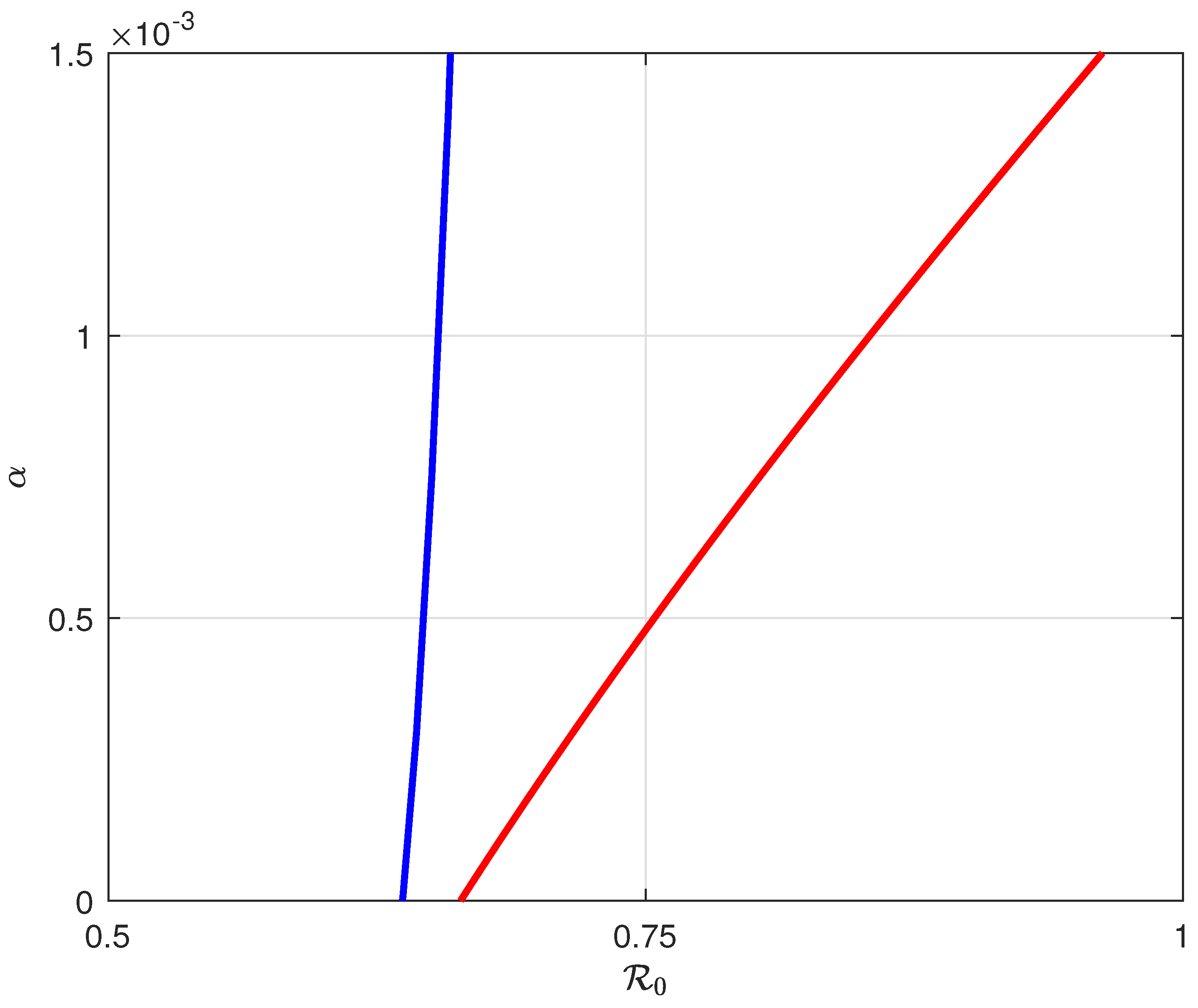
Next, we present the results of a sensitivity analysis for the effect of some model parameters on the range of the backward bifurcation. We limit our analysis to the model parameters for which baseline values are not known. We start with α , that represents the effect of individuals’ fear of the disease. We plotted in the same diagram the locus of the limit point and the Hopf point. It can be seen (Figure 2) that while the locus of the limit point is largely insensitive to changes in α , the locus of the Hopf point increases almost linearly and approaches R 0 = 1 . This implies, as expected, that as the fear effect increases, it is much easier to eradicate the disease since the region of bistability between the Hopf point and R 0 = 1 becomes narrower. Moreover, the diagram shows the existence of a backward bifurcation (with a limit and Hopf points) even when there is no fear of the disease, i.e., α = 0 .
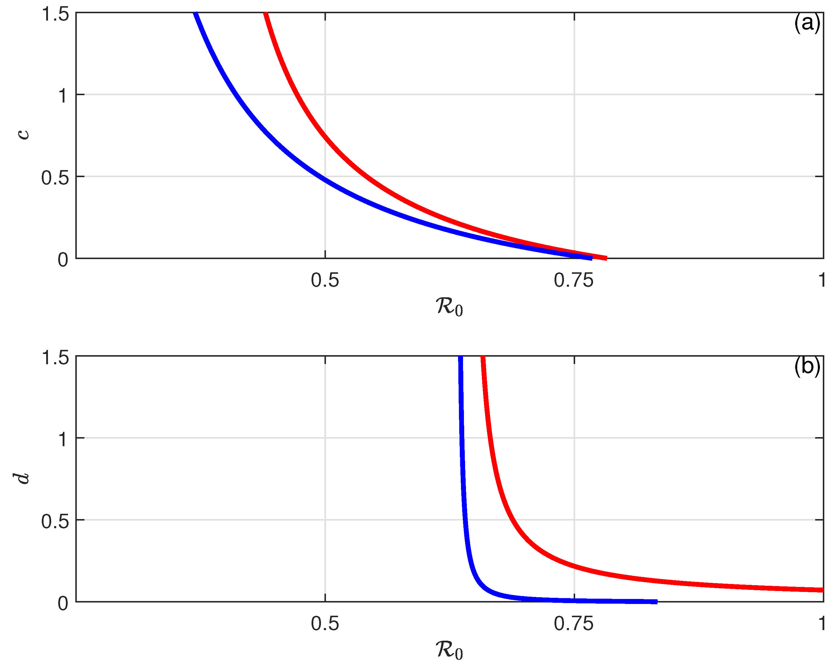
The effect of the first parameter c of the treatment function c I 1 + d I is shown in Figure 3a. It can be seen that as c increases, both the LP and the HB points move to smaller values of R 0 , and the range between them in terms of R 0 increases. But this is only one element of the picture. Figure 3b shows the effect of d, the second parameter of the treatment function. It can be seen that as d increases (and the inhibition 1 1 + d I is reduced), both the limit and Hopf points move closer to R 0 = 1 , making it easier to eradicate the disease.
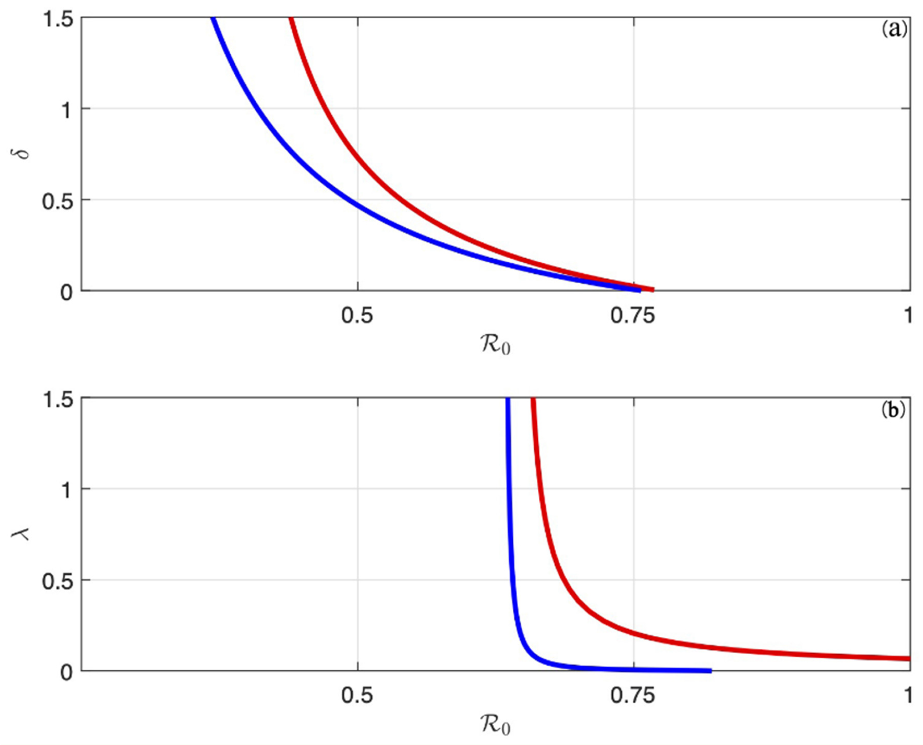
The effect of the maximum recovery rate is shown in Figure 4a. As δ increases, we can see that both the Hopf points and the limit points move to smaller values of R 0 . But again, there is also another element of the picture shown in Figure 4b. If the quality of health services λ increases, the Hopf points and the limit points reach values closer to unity and the bistability region is reduced substantially.
It is normal that the effect of λ is comparable to the effect of d in the treatment function c I 1 + d I and the effect of the difference δ between the maximum recovery rate γ 0 + δ and the minimum recovery rate γ 0 is also similar to that of c.
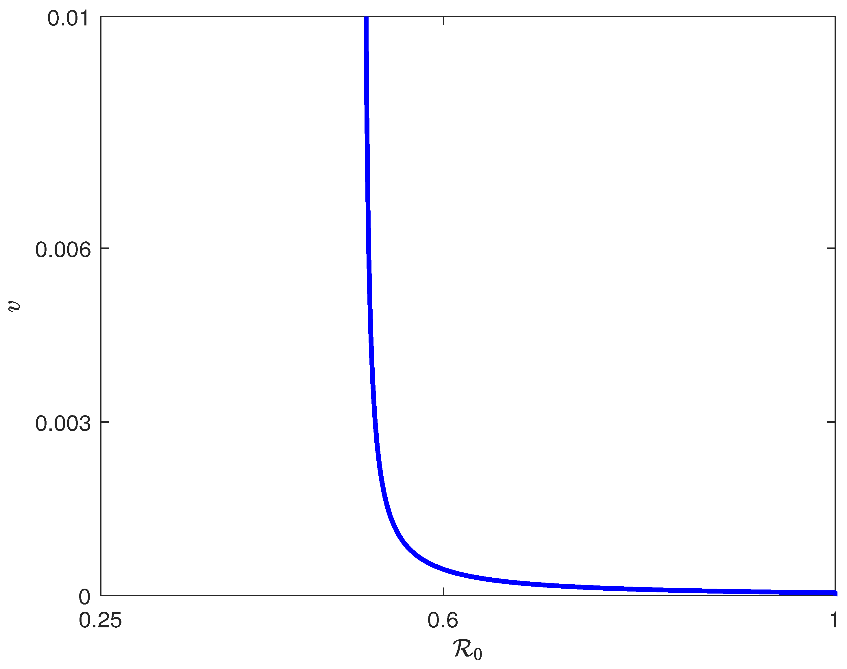
Finally, the effect of vaccination is shown in Figure 5. Our numerical analysis showed that the Hopf point occurs for a very small range of dimensional vaccination rate, i.e., between 0.000291 and 0.000301 (the nominal dimensional value being 0.00030). Its occurrence is therefore not significant and its locus is not shown in the figure. Figure 4 also shows that when the vaccination rate is very small, the locus of the limit point moves to R 0 = 1 ; however, when the vaccination rate increases, the location of the limit point decreases in term of R 0 . Past a critical value, the locus of the limit point becomes insensitive to changes in the vaccination rate.
It is worth comparing the results of our work to other similar SIER models. For instance, the investigation in [25] analyzed the impact of hospital bed availability on recovery rates. The results revealed that a variable recovery rate led to more sophisticated dynamics such as cusp-type Bogdanov–Takens bifurcation. While our model did not predict this specific behavior, it effectively anticipated other dynamics, including backward bifurcation and Hopf bifurcation.
In relation to the research on the effects of fear [23], our model successfully predicted the occurrence of a backward bifurcation at certain levels of fear. This indicates that the critical value of the reproduction number at the limit point can serve as a novel threshold for managing disease control.

9. Conclusions

This research introduced and evaluated the dynamics of an SEIR model focused on the transmission of seasonal influenza, featuring four key enhancements: (1) the integration of a fear factor, (2) a recovery rate that is nonlinear and contingent upon the quality of health services, (3) a nonlinear treatment function, and (4) a basic vaccination rate. Most parameters of the model were either extracted from scholarly sources or gathered from data specific to Saudi Arabia.
Our analysis of backward bifurcation revealed two noteworthy behaviors: (1) a static coexistence of the endemic equilibrium alongside the disease-free solution occurs when the reproduction number is between the Hopf point and unity, and (2) a lack of stable oscillatory behavior.
The research revealed that the range of backward bifurcation can be diminished by elevating the quality of health services, decreasing treatment delays, and enhancing the fear effect. The latter can be effectively achieved by promoting education and awareness through various media outlets.
Based on the current study, we recommend two potential areas for further investigation. The model’s accuracy could be enhanced by adjusting its parameters. For example, the virus’s death rate does not adequately consider important factors such as age, with older adults being more significantly impacted than younger individuals, as well as the existing health conditions of patients. Furthermore, the model could be refined by allowing certain parameters, such as the transmission rates β 1 , β 2 , and the fear level, to vary over time. The fear level, in particular, is unlikely to remain constant, as it is affected by the disease’s severity and the death toll.

Author Contributions

Conceptualization, A.A. and R.T.A.; methodology, A.A., R.T.A., and M.A.; software, A.A. and R.T.A.; validation, A.A. and R.T.A.; formal analysis, A.A. and R.T.A.; resources R.T.A. and M.A.; writing—original draft preparation, A.A., R.T.A., and M.A.; project administration, R.T.A.; funding acquisition, R.T.A. All authors have read and agreed to the published version of the manuscript.

Funding

This work was supported and funded by the Deanship of Scientific Research at Imam Mohammad Ibn Saud Islamic University (IMSIU) (grant number IMSIU-DDRSP2501).

Data Availability Statement

The original contributions presented in the study are included in the article. Further inquires can be directed to the corresponding author.

Conflicts of Interest

The authors declare no conflicts of interest. The funders had no role in the design of the study; in the collection, analyses, or interpretation of data; in the writing of the manuscript; or in the decision to publish the results.

Appendix A

  • Existence and uniqueness: The right-hand side of the system (Equations (9)–(12)) is continuous and differentiable on R + 4 = { ( S , E , I , R ) : S 0 , E 0 , I 0 , R 0 } and hence locally Lipschitzian. Therefore, the solution ( S ( t ) , E ( t ) , I ( t ) , R ( t ) ) of the model with initial conditions S ( 0 ) 0 , E ( 0 ) 0 , I ( 0 ) 0 , C ( 0 ) 0 exists and it is unique. We can write Equation (9) as follows:
    d S ( t ) d t = 1 1 + α I S ( t ) ξ ( t ) ,
    where
    ξ ( t ) = β 1 I + β 2 E + μ + v .
    Using the integrating factor method, integrating Equations (A1) and (A2) yields
    S t = 0 t Λ 1 + α I ( η ) e 0 η ξ ζ d ζ d η + S 0 0 t e 0 t ξ η d η d t > 0 .
    Thus, S ( t ) is positive for all t.
    For the proofs that E ( t ) and I ( t ) are positive, we divide this issue into four cases:
    • E 0 = I 0 = 0 . From Equations (10) and (11), we can see E ( t ) = I ( t ) = 0 for all t 0 .
    • E 0 > 0 and I 0 = 0 . Since E ( t ) is continuous at t = 0 and since d I d t ( t = 0 ) = a E 0 > 0 , we conclude that E ( t ) > 0 and I ( t ) > 0 for all t 0 . If this is not true, then we can choose
      t 1 = inf t : E ( t ) = 0 or I ( t ) = 0 ( 0 , ) .
      If E ( t 1 ) = 0 , then since d E d t ( μ + a ) E 0 for 0 t t 1 , we conclude that
      E ( t 1 ) E 0 e ( μ + a ) t 1 > 0 ,
      which contradicts the assumption that E ( t 1 ) = 0 .
      If, on the other hand, I ( t 1 ) = 0 , then there exists θ such that t 1 > θ and 0 < I ( t ) < ψ on [ t 1 θ , t 1 ) . Equation (11) implies, since c I 1 + d I < c I and γ 0 + δ 1 + λ I < γ 0 + δ , that
      d I d t μ + μ 1 + γ 0 + δ + c I .
      This gives
      I ( t 1 ) I ( t 1 θ ) e ( t 1 θ ) t 1 ( μ + μ 1 + γ 0 + δ + c ) d u > 0 ,
      which also contradicts the assumption that I ( t 1 ) = 0 . The same analysis can be carried out for the other cases: ( E 0 = 0 , I 0 > 0 ) and ( E 0 > 0 , I 0 > 0 ) . We conclude, therefore, that E ( t ) and I ( t ) are positive for all t 0 .
      Next, since we showed that S ( t ) > 0 and I ( t ) > 0 , we can deduce from Equation (12) that
      d R ( t ) d t μ R ( t ) .
      This yields
      R ( t ) R 0 e 0 t ( μ ) d τ < 0 .
      This proves that R ( t ) > 0 .
  • Boundedness The compact set Ψ , defined by
    Ψ = { ( S ( t ) , E ( t ) , I ( t ) , R ( t ) ) I R + 4 , S ( t ) + E ( t ) + I ( t ) + R ( t ) 1 μ } ,
    where ( S ( t ) , E ( t ) , I ( t ) , R ( t ) ) are the solutions of the model (Equations (9)–(13)) with initial conditions ( S 0 , E 0 , I 0 , R 0 ), is a positively invariant region. Let us denote that N ( t ) = S ( t ) + E ( t ) + I ( t ) + R ( t ) . We then have from Equations (9)–(13) that
    d N ( t ) d t = μ N ( t ) μ 1 I + 1 1 + α I .
    Therefore,
    d N ( t ) d t μ N ( t ) + 1 1 + α I μ N ( t ) + 1 ,
    Integrating Equation (A11) yields
    N ( t ) N ( 0 ) exp ( μ t ) + 1 μ ( 1 exp ( μ t ) ) ,
    where N ( 0 ) is the initial condition of N ( t ) . Therefore, 0 < N ( t ) < 1 μ as t goes to + and d N ( t ) d t < 0 for N > 1 μ . This shows that Ψ is positively invariant.

Appendix B

Coefficients of the polynomial equation F ( I ) : = a 6 I 6 + a 5 I 5 + a 4 I 4 + a 3 I 3 + a 2 I 2 + a 1 I + a 0 = 0 .
a 6 = α d 2 ( a + μ ) ( γ 0 + μ + μ 1 ) ( a β 1 + β 2 ( γ 0 + μ + μ 1 ) ) λ 2 . a 5 = d ( a + μ ) λ ( a α β 1 d ( δ + 2 ( γ 0 + μ + μ 1 ) ) + a ( β 1 d ( γ 0 + μ + μ 1 ) + α ( β 1 ( c + 2 ( γ 0 + μ + μ 1 ) ) + d ( γ 0 + μ + μ 1 ) ( μ + v ) ) ) λ + β 2 ( γ 0 + μ + μ 1 ) ( d ( γ 0 + μ + μ 1 ) λ + 2 α ( d ( δ + γ 0 + μ + μ 1 ) + ( c + γ 0 + μ + μ 1 ) λ ) ) ) .
a 4 = β 2 μ ( 2 d ( γ 0 + μ + m u 1 ) x l ( d ( δ + γ 0 + μ + μ 1 ) + ( c + γ 0 + μ + μ 1 ) λ ) + α ( d 2 ( δ + γ 0 + μ + μ 1 ) 2 + 2 d ( 2 ( γ 0 + μ + μ 1 ) ( δ + γ 0 + μ + μ 1 ) + c ( δ + 2 ( γ 0 + μ + μ 1 ) ) ) λ + ( c + γ 0 + μ + μ 1 ) 2 λ 2 ) ) a 2 ( d λ ( d ( γ 0 + μ + μ 1 ) ( μ + v ) λ + β 1 ( d ( δ + 2 ( γ 0 + μ + μ 1 ) λ ) + ( c + 2 ( γ 0 + μ + μ 1 ) ) λ ) ) + α ( d ( μ + v ) λ ( d ( δ + 2 ( γ 0 + μ + μ 1 ) ) + ( c + 2 ( γ 0 + μ + μ 1 ) ) λ ) + β 1 ( d 2 ( δ + γ 0 + μ + μ 1 ) + 2 d ( c + δ + 2 ( γ 0 + μ + μ 1 ) ) λ + ( c + γ 0 + μ + μ 1 ) λ 2 ) ) ) a ( d λ ( d μ ( γ 0 + μ + μ 1 ) ( μ + v ) λ + β 2 ( γ 0 + μ + μ 1 ) ( 2 d ( δ + γ 0 + μ + μ 1 ) d λ + 2 ( c + γ 0 + μ + μ 1 ) λ ) + β 1 μ ( d ( δ + 2 ( γ 0 + μ + μ 1 ) ) + ( c + 2 ( γ 0 + μ + μ 1 ) ) λ ) ) + α ( β 2 ( d 2 ( δ + γ 0 + μ + μ 1 ) 2 + 2 d ( 2 ( γ 0 + μ + μ 1 ) ( δ + γ 0 + μ + μ 1 ) + c ( δ + 2 ( γ 0 + μ + μ 1 ) ) ) λ + ( c + γ 0 + μ + μ 1 ) 2 λ 2 ) + μ ( d ( μ + v ) λ ( d ( δ + 2 ( γ 0 + μ + μ 1 ) ) + ( c + 2 ( γ 0 + μ + μ 1 ) ) λ ) + β 1 ( d 2 ( δ + γ 0 + μ + μ 1 ) + 2 d ( c + δ + 2 ( γ 0 + μ + μ 1 ) ) λ + ( c + γ 0 + μ + μ 1 ) λ 2 ) ) ) )
a 3 = β 2 μ ( d 2 ( δ + γ 0 + μ + μ 1 ) 2 + 2 d ( 2 ( γ 0 + μ + μ 1 ) ( δ + γ 0 + μ + μ 1 ) + c ( δ + 2 ( γ 0 + μ + μ 1 ) ) ) λ + ( c + γ 0 + μ + μ 1 ) 2 λ 2 + 2 α ( c + δ + γ 0 + μ + μ 1 ) ( d ( δ + γ 0 + μ + μ 1 ) + ( c + γ 0 + μ + μ 1 ) λ ) ) a 2 ( d ( μ + v ) λ ( d ( δ + 2 ( γ 0 + μ + μ 1 ) ) + ( c + 2 ( γ 0 + μ + μ 1 ) ) λ ) + β 1 ( d 2 ( δ + γ 0 + μ + μ 1 ) + 2 d ( c d + δ + 2 ( γ 0 + μ + μ 1 ) ) λ + ( c 2 d + γ 0 + μ + μ 1 ) λ 2 ) + α ( β 1 d ( c + 2 ( δ + γ 0 + μ + μ 1 ) ) + β 1 ( 2 c + δ + 2 ( γ 0 + μ + μ 1 ) ) λ + ( μ + v ) ( d 2 ( δ + γ 0 + μ + μ 1 ) + 2 d ( c + δ + 2 ( γ 0 + μ + μ 1 ) ) λ + ( c + γ 0 + μ + μ 1 ) λ 2 ) ) ) a ( β 2 ( d ( c ( 2 δ + 4 ( γ 0 + μ + μ 1 ) λ ) + 2 ( γ 0 + μ + μ 1 ) ( 2 ( δ + γ 0 + μ + μ 1 ) λ ) ) λ + ( c + γ 0 + μ + μ 1 ) 2 λ 2 + d 2 ( ( δ + γ 0 + μ + μ 1 ) 2 ( δ + 2 ( γ 0 + μ + μ 1 ) ) λ ) ) + μ ( d ( μ + v ) λ ( d ( δ + 2 ( γ 0 + μ + μ 1 ) ) + ( c + 2 ( γ 0 + μ + μ 1 ) ) λ ) + β 1 ( d 2 ( δ + γ 0 + μ + μ 1 ) + 2 d ( c + δ + 2 ( γ 0 + μ + μ 1 ) ) λ + ( c + γ 0 + μ + μ 1 ) λ 2 ) ) + α ( 2 β 2 ( c + δ + γ 0 + μ + μ 1 ) ( d ( δ + γ 0 + μ + μ 1 ) + ( c + γ 0 + μ + μ 1 ) λ ) + μ ( β 1 d ( c + 2 ( δ + γ 0 + μ + μ 1 ) ) + β 1 ( 2 c + δ + 2 ( γ 0 + μ + μ 1 ) ) λ + ( μ + v ) ( d 2 ( δ + γ 0 + μ + μ 1 ) + 2 d ( c + δ + 2 ( γ 0 + μ + μ 1 ) ) λ + ( c + γ 0 + μ + μ 1 ) λ 2 ) ) ) )
a 2 = β 2 μ ( c + δ + γ 0 + μ + μ 1 ) ( 2 d ( δ + γ 0 + μ + μ 1 ) + α ( c + δ + γ 0 + μ + μ 1 ) + 2 ( c + γ 0 + μ + μ 1 ) λ ) a 2 ( β 1 ( d ( c d + 2 ( δ + γ 0 + μ + μ 1 ) ) + ( 2 c 4 d + δ + 2 ( γ 0 + μ + μ 1 ) ) λ λ 2 ) + ( μ + v ) ( d 2 ( δ + γ 0 + μ + μ 1 ) + 2 d ( c + δ + 2 ( γ 0 + μ + μ 1 ) ) λ + ( c + γ 0 + μ + μ 1 ) λ 2 ) + α ( β 1 ( c + δ + γ 0 + μ + μ 1 ) + ( μ + v ) ( d ( c + 2 ( δ + γ 0 + μ + μ 1 ) ) + ( 2 c + δ + 2 ( γ 0 + μ + μ 1 ) ) λ ) ) ) a ( β 2 ( d 2 ( δ + γ 0 + μ + μ 1 ) + 2 c 2 λ + ( γ 0 + μ + μ 1 ) ( 2 ( δ + γ 0 + μ + μ 1 ) λ ) λ + 2 d ( ( δ + γ 0 + μ + μ 1 ) 2 ( δ + 2 ( γ 0 + μ + μ 1 ) ) λ ) + c ( 2 d ( δ + γ 0 + μ + μ 1 λ ) + ( 2 δ + 4 ( γ 0 + μ + μ 1 ) λ ) λ ) ) + μ ( β 1 d ( c + 2 ( δ + γ 0 + μ + μ 1 ) ) + β 1 ( 2 c + δ + 2 ( γ 0 + μ + μ 1 ) ) λ + ( μ + v ) ( d 2 ( δ + γ 0 + μ + μ 1 ) + 2 d ( c + δ + 2 ( γ 0 + μ + μ 1 ) ) λ + ( c + γ 0 + μ + μ 1 ) λ 2 ) ) + α ( β 2 ( c + δ + γ 0 + μ + μ 1 ) 2 + μ ( β 1 ( c + δ + γ 0 + μ + μ 1 ) + ( μ + v ) ( d ( c + 2 ( δ + γ 0 + μ + μ 1 ) ) + ( 2 c + δ + 2 ( γ 0 + μ + μ 1 ) ) λ ) ) ) )
a 1 = β 2 μ ( c + δ + γ 0 + μ + μ 1 ) 2 a 2 ( β 1 ( c 2 d + δ + γ 0 + μ + μ 1 2 λ ) + ( μ + v ) ( α ( c + δ + γ 0 + μ + μ 1 ) + d ( c + 2 ( δ + γ 0 + μ + μ 1 ) ) + ( 2 c + δ + 2 ( γ 0 + μ + μ 1 ) ) λ ) ) a ( β 2 ( c 2 2 d ( δ + γ 0 + μ + μ 1 ) + ( δ + γ 0 + μ + μ 1 ) 2 + c ( d + 2 ( δ + γ 0 + μ + μ 1 λ ) ) ( δ + 2 ( γ 0 + μ + μ 1 ) ) λ ) + μ ( β 1 ( c + δ + γ 0 + μ + μ 1 ) + ( μ + v ) ( α ( c + δ + γ 0 + μ + μ 1 ) + d ( c + 2 ( δ + γ 0 + μ + μ 1 ) ) + ( 2 c + δ + 2 ( γ 0 + μ + μ 1 ) ) λ ) ) )
a 0 = a ( ( c + δ + γ 0 + μ + μ 1 ) ( β 2 + μ ( μ + v ) ) + a ( β 1 ( c + δ + γ 0 + μ + μ 1 ) ( μ + v ) ) )

References

  1. World Health Organization. Available online: https://www.who.int/ (accessed on 10 April 2025).
  2. Iuliano, A.D.; Roguski, K.M.; Chang, H.H.; Muscatello, D.J.; Palekar, R.; Tempia, S.; Cohen, C.; Gran, J.M.; Schanzer, D.; Cowling, B.J.; et al. Estimates of global seasonal influenza-associated respiratory mortality: A modelling study. Lancet 2018, 391, 1285. [Google Scholar] [CrossRef] [PubMed]
  3. Chakraborty, S.; Chauhan, A. Fighting the flu: A brief review on anti-influenza agents. Biotechnol. Genet. Eng. Rev. 2023, 40, 858. [Google Scholar] [CrossRef]
  4. Gao, Y.; Guyatt, G.; Uyeki, T.M.; Liu, M.; Chen, Y.; Zhao, Y.; Shen, Y.; Xu, J.; Zheng, Q.; Li, Z.; et al. Antivirals for treatment of severe influenza: A systematic review and network meta-analysis of randomised controlled trials. Lancet 2024, 404, 753. [Google Scholar] [CrossRef]
  5. Quirouette, C.; Younis, N.P.; Reddy, M.B.; Beauchemin, C.A. A mathematical model describing the localization and spread of influenza A virus infection within the human respiratory tract. PLoS Comput. Biol. 2020, 16, e1007705. [Google Scholar]
  6. Zhao, Z.; Zhai, M.; Li, G.; Gao, X.; Song, W.; Wang, X.; Ren, H.; Cui, Y.; Qiao, Y.; Ren, J.; et al. Study on the prediction effect of a combined model of SARIMA and LSTM based on SSA for influenza in Shanxi Province, China. BMC Infect. Dis. 2023, 23, 71. [Google Scholar] [CrossRef]
  7. Modnak, C.; Wang, J. Optimal treatment strategy of an avian influenza model with latency. Int. J. Biomath. 2017, 10, 1750066. [Google Scholar] [CrossRef]
  8. Shi, W.W.; Tan, Y.S. Transmission dynamics and optimal control of an influenza model with quarantine and treatment. Int. J. Biomath. 2012, 5, 1260011. [Google Scholar] [CrossRef]
  9. Baba, I.A.; Ahmad, H.; Alsulami, M.D.; Abualnaja, K.M.; Altanji, M. A mathematical model to study resistance and non-resistance strains of influenza. Results Phys. 2021, 26, 104390. [Google Scholar] [CrossRef]
  10. Mathur, K.S.; Narayan, P. Dynamics of an SVEIRS epidemic model with vaccination and saturated incidence rate. Int. J. Appl. Comput. Math. 2018, 4, 118. [Google Scholar] [CrossRef]
  11. Mohammad, K.M.; Akhi, A.A.; Kamrujjaman, M. Bifurcation analysis of an influenza A (H1N1) model with treatment and vaccination. PLoS ONE 2025, 20, e0315280. [Google Scholar] [CrossRef]
  12. Osthus, D.; Hickmann, K.S.; Caragea, P.C.; Higdon, D.; Del Valle, S.Y. Forecasting seasonal influenza with a state-space SIR model. Forecasting seasonal influenza with a state-space SIR model. Ann. Appl. Stat. 2017, 11, 202. [Google Scholar] [CrossRef] [PubMed]
  13. Sabir, Z.; Said, S.B.; Al-Mdallal, Q. A fractional order numerical study for the influenza disease mathematical model. Alex. Eng. J. 2023, 65, 615. [Google Scholar] [CrossRef]
  14. Evirgen, F.; Uçar, E.; Uçar, S.; Özdemir, N. Modelling Influenza A disease dynamics under Caputo-Fabrizio fractional derivative with distinct contact rates. Math. Model. Numer. Simul. Appl. 2023, 3, 58. [Google Scholar] [CrossRef]
  15. Alzahrani, S.M.; Saadeh, R.; Abdoon, M.A.; Qazza, A.; EL Guma, F.; Berir, M. Numerical simulation of an influenza epidemic: Prediction with fractional SEIR and the ARIMA model. Appl. Math. Inf. Sci. 2024, 18, 1. [Google Scholar]
  16. Chen, Y.; Zhang, J.; Jin, Z. Optimal control of an influenza model with mixed cross-infection by age group. Math. Comput. Simul. 2023, 206, 410. [Google Scholar] [CrossRef]
  17. Samanta, G.P. Global dynamics of a nonautonomous SIRC model for influenza A with distributed time delay. Differ. Equ. Dyn. Syst. 2010, 18, 341. [Google Scholar] [CrossRef]
  18. Sabir, Z.; Botmart, T.; Raja, M.A.Z.; Sadat, R.; Ali, M.R.; Alsulami, A.A.; Alghamdi, A. Artificial neural network scheme to solve the nonlinear influenza disease model. Biomed. Signal Process. Control 2022, 75, 103594. [Google Scholar] [CrossRef]
  19. Epstein, J.M.; Parker, J.; Cummings, D.; Hammond, R.A. Coupled contagion dynamics of fear and disease: Mathematical and computational explorations. PLoS ONE 2008, 3, e3955. [Google Scholar] [CrossRef] [PubMed]
  20. Valle, S.; Mniszewski, S.; Hyman, J. Modeling the impact of behavior changes on the spread of pandemic influenza. In Modeling the Interplay Between Human Behavior and the Spread of Infectious Diseases; Manfredi, P., d’Onofrio, A., Eds.; Springer Science Business Media: New York, NY, USA, 2012; pp. 59–77. [Google Scholar]
  21. Mpeshe, S.C.; Nyerere, N. Modeling the dynamics of coronavirus disease pandemic coupled with fear epidemics. Comput. Math. Methods Med. 2021, 2021, 6647425. [Google Scholar] [CrossRef]
  22. Maji, C. Impact of media-induced fear on the control of COVID-19 outbreak: A mathematical study. Int. J. Differ. Equ. 2021, 2021, 2129490. [Google Scholar] [CrossRef]
  23. Thirthar, A.A.; Abboubakar, H.; Khan, A.; Abdeljawad, T. Mathematical modeling of the COVID-19 epidemic with fear impact. J. AIMS Math. 2023, 8, 6447. [Google Scholar] [CrossRef]
  24. Zhang, X.; Liu, X. Backward bifurcation of an epidemic model with saturated treatment. J. Math. Anal. Appl. 2008, 348, 433. [Google Scholar] [CrossRef]
  25. Chan, C.; Zhu, H. Bifurcations and complex dynamics of an SIR model with the impact of the number of hospital beds. J. Diff. Equ. 2014, 257, 1662. [Google Scholar]
  26. Wang, W. Backward bifurcation of an epidemic model with treatment. Math. Biosci. 2006, 201, 58. [Google Scholar] [CrossRef]
  27. Candelli, M.; Pignataro, G.; Torelli, E.; Gullì, A.; Nista, E.C.; Petrucci, M.; Saviano, A.; Marchesini, D.; Covino, M.; Ojetti, V.; et al. Effect of influenza vaccine on COVID-19 mortality: A retrospective study. Intern. Emerg. Med. 2021, 16, 1849. [Google Scholar]
  28. Van den Driessche, P.; Watmough, J. Reproduction numbers and subthreshold endemic equilibria for compartmental models of disease transmission. Math. Biosci. 2002, 180, 29. [Google Scholar] [CrossRef] [PubMed]
  29. Castillo-Chavez, C.; Song, B. Dynamical models of tuberculosis and their applications. Math. Biosci. Eng. 2004, 1, 361. [Google Scholar] [CrossRef]
  30. General Authority for Statistics in Saudi Arabia. Statistics Library. Available online: https://www.stats.gov.sa/en/statistics?index=119025 (accessed on 10 April 2025).
  31. Alshahrani, A.M.; Okmi, E.; Sullivan, S.G.; Tempia, S.; Barakat, A.; Naja, H.A.E.; Aman, A.; Hamedelneil, O.; Mohamed, M.; Basheer, S.F.; et al. Uncovering the burden of influenza-associated illness across levels of severity in the kingdom of Saudi Arabia across three seasons. J. Epidemiol. Glob. Health 2025, 15, 47. [Google Scholar] [CrossRef]
  32. Carcione, J.M.; Santos, J.E.; Bagaini, C.; Ba, J. A Simulation of a COVID-19 Epidemic Based on a Deterministic SEIR Model. Front. Public Health 2020, 8, 230. [Google Scholar] [CrossRef]
  33. Dhooge, A.; Govaerts, W.; Kuznetsov, Y.A.; Meijer, H.G.E.; Sautois, B. New features of the software MatCont for bifurcation analysis of dynamical systems. Math. Comput. Model. Dyn. Syst. 2008, 14, 147. [Google Scholar] [CrossRef]
  34. MATLAB. Version 9.4.0 (R2018a); The MathWorks Inc.: Natick, MA, USA, 2018. [Google Scholar]
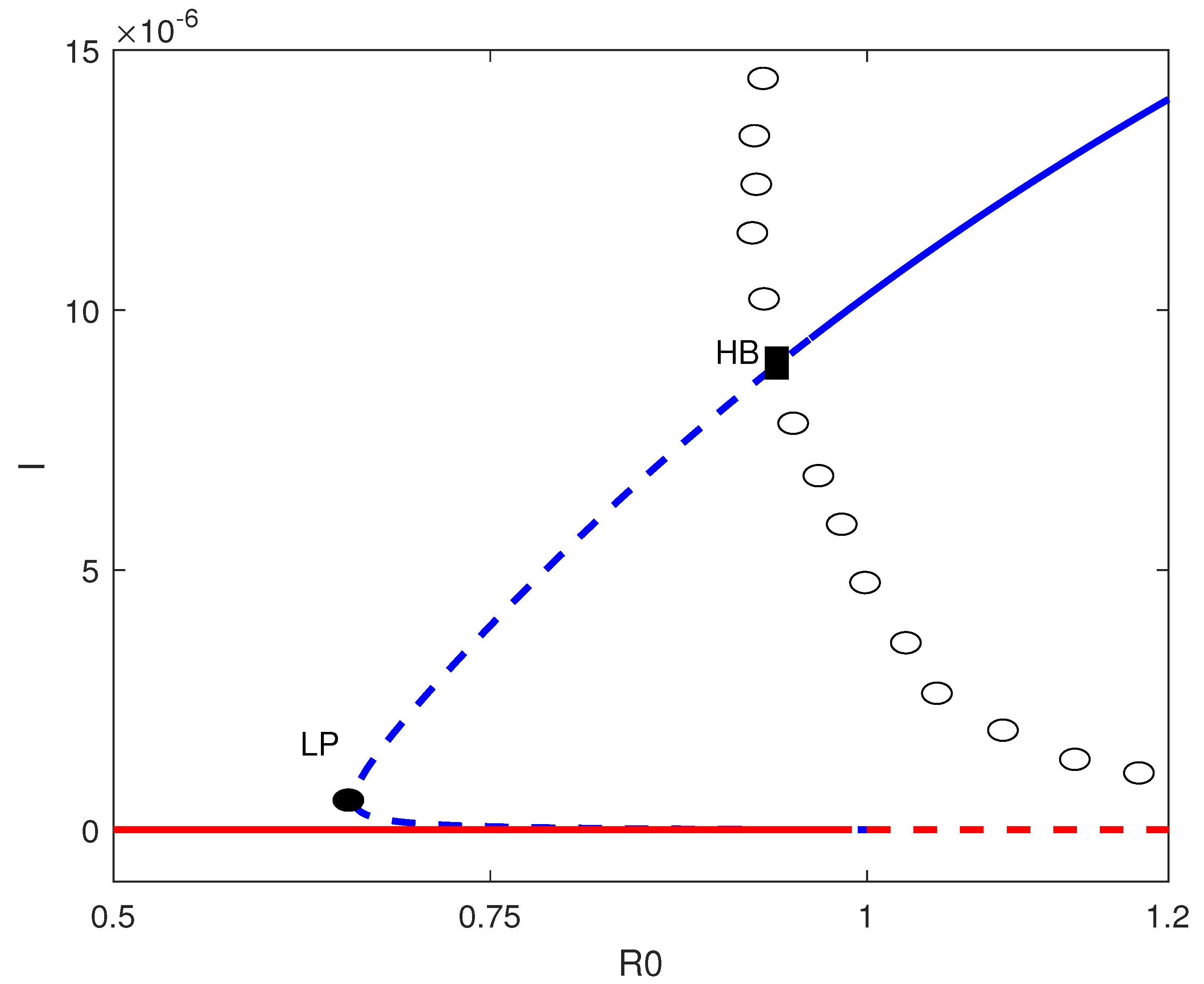
Figure 1. Bifurcation diagram for α = 0.0001 and the rest of the model parameters in Equation (72), showing backward bifurcation. Solid line (stable branch); dashed line (unstable branch); LP (static limit point); HB (Hopf point); blue line (endemic solution); red line (disease-free solution); circles (unstable periodic branches).
Symmetry 17 00803 g001
Figure 2. Two-parameter continuation diagrams showing the locus of the limit point (blue) and Hopf point (red) of Figure 1 in the parameter space ( R 0 , α ) .
Symmetry 17 00803 g002
Figure 3. Two-parameter continuation diagrams showing the locus of the limit point (blue) and Hopf point (red) of Figure 1 in the parameter spaces (a) ( R 0 , c ) and (b) ( R 0 , d ) .
Symmetry 17 00803 g003
Figure 4. Two-parameter continuation diagrams showing the locus of the limit point (blue) and Hopf point (red) of Figure 1 in the parameter spaces (a) ( R 0 , δ ) and (b) ( R 0 , λ ) .
Symmetry 17 00803 g004
Figure 5. Two-parameter continuation diagram showing the locus of the limit point of Figure 1 in the parameter space ( R 0 , v ) .
Symmetry 17 00803 g005
Table 1. Number of positive real roots of Equation (24).
Case a 6 a 5 a 4 a 3 a 2 a 1 a 0 R 0 Number of Sign ChangesNumber of Positive Roots
1−1−1−1−1−1−1−1 R 0 < 1 00
2−1−1−1−1−1−11 R 0 > 1 11
3−1−1−1−1−11−1 R 0 < 1 22, 0
4−1−1−1−1−111 R 0 > 1 11
5−1−1−1−11−1−1 R 0 < 1 22, 0
6−1−1−1−11−11 R 0 > 1 33, 1
7−1−1−1−111−1 R 0 < 1 22, 0
8−1−1−1−1111 R 0 > 1 11
9−1−1−11−1−1−1 R 0 < 1 22, 0
10−1−1−11−1−11 R 0 > 1 33, 1
11−1−1−11−11−1 R 0 < 1 44, 2, 0
12−1−1−11−111 R 0 > 1 33, 1
13−1−1−111−1−1 R 0 < 1 22, 0
14−1−1−111−11 R 0 > 1 33, 1
15−1−1−1111−1 R 0 < 1 22, 0
16−1−1−11111 R 0 > 1 11
17−1−11−1−1−1−1 R 0 < 1 22, 0
18−1−11−1−1−11 R 0 > 1 33, 1
19−1−11−1−11−1 R 0 < 1 44, 2, 0
20−1−11−1−111 R 0 > 1 33,1
21−1−11−11−1−1 R 0 < 1 44, 2, 0
22−1−11−11−11 R 0 > 1 44, 2, 0
23−1−11−111−1 R 0 < 1 44, 2, 0
24−1−11−1111 R 0 > 1 33, 1
25−1−111−1−1−1 R 0 < 1 22, 0
26−1−111−1−11 R 0 > 1 33, 1
27−1−111−11−1 R 0 < 1 44, 2, 0
28−1−111−111 R 0 > 1 22, 0
29−1−1111−1−1 R 0 < 1 22, 0
30−1−1111−11 R 0 > 1 33, 1
31−1−11111−1 R 0 < 1 22, 0
32−1−111111 R 0 > 1 11
Disclaimer/Publisher’s Note: The statements, opinions and data contained in all publications are solely those of the individual author(s) and contributor(s) and not of MDPI and/or the editor(s). MDPI and/or the editor(s) disclaim responsibility for any injury to people or property resulting from any ideas, methods, instructions or products referred to in the content.