Adaptive Network-Based Fuzzy Inference System Training Using Nine Different Metaheuristic Optimization Algorithms for Time-Series Analysis of Brent Oil Price and Detailed Performance Analysis

Abstract

Brent oil holds a significant position in the global energy market, as oil prices in many regions are indexed to it. Therefore, forecasting the future price of Brent oil is of great importance. In recent years, artificial intelligence techniques have been widely applied in modeling and prediction tasks. In this study, an Adaptive Neuro-Fuzzy Inference System (ANFIS), a well-established AI approach, was employed for the time-series forecasting of Brent oil prices. To ensure effective learning and improve prediction accuracy, ANFIS was trained using nine different metaheuristic algorithms: Artificial Bee Colony (ABC), Selfish Herd Optimizer (SHO), Biogeography-Based Optimization (BBO), Multi-Verse Optimizer (MVO), Teaching–Learning-Based Optimization (TLBO), Cuckoo Search (CS), Moth Flame Optimization (MFO), Marine Predator Algorithm (MPA), and Flower Pollination Algorithm (FPA). Symmetric training procedures were applied across all algorithms to ensure fair and consistent evaluation. The analyses were conducted on the lowest and highest daily, weekly, and monthly Brent oil prices. Mean squared error (MSE) was used as the primary performance metric. The results showed that all algorithms achieved effective prediction performance. Among them, BBO and TLBO demonstrated superior accuracy and stability, particularly in handling the complexities of Brent oil forecasting. This study contributes to the literature by combining ANFIS and metaheuristics within a symmetric framework of experimentation and evaluation.

1. Introduction

For many years, crude oil has been one of the most significant energy and financial assets in the world and continues to be so. Roughly one-third of the world’s energy is derived from crude oil, which may be refined into a variety of fuels to satisfy varied consumer needs [1]. It is also a common raw material for petroleum-based items in daily life. Since fluctuations in the price of crude oil have a domino effect on the global economy, forecasting its price is crucial for planning long-term strategies. Because of its very volatile and turbulent structure—which is especially influenced by politics—accurate prediction-making is crucial [1,2]. In order to make our predictions, we must first discuss artificial intelligence, an area of study that has seen significant growth in popularity recently and has been employed widely. The primary methods of artificial intelligence include heuristic optimization algorithms, fuzzy logic, artificial neural networks, and neuro-fuzzy systems. Numerous issues in the actual world have been resolved with them [3,4,5]. Fuzzy sets and inference systems are the most preferred approach for solving ambiguous and imprecise situations [6]. However, it is crucial to keep in mind that they are unable to make rules on their own or carry out the learning process [7]. Nonetheless, self-organization, self-interaction, and environmental learning are all possible with artificial neural networks (ANNs) [8]. The Adaptive Network-Based Fuzzy Inference System (ANFIS) [9], which integrates the characteristics of artificial neural networks and fuzzy inference systems, is one of the most well-known neuro-fuzzy systems. It combines the best features of both systems: fuzzy, which performs well in mapping via membership functions and alpha cuts, and ANN, which is great at self-organizing [5,8]. Hence, it provides a reliable approach to problem modeling and identification.

2. Literature Review

During the past few decades, forecasting the price of crude oil has made extensive use of conventional statistical and econometric methods [10,11]. Amano made one of the first study proposals about oil market forecasting [12]. The author predicted the oil market using a small-scale econometric model. In order to forecast crude oil prices in the 1980s, Huntington used an advanced econometric model [13]. Furthermore, a probabilistic model was used by Abramson and Finizza to forecast oil prices [14]. When the price series being studied is linear or nearly linear, the models mentioned above can produce accurate forecast results. However, there is a significant amount of nonlinearity and irregularity in real-world crude oil price series [10,11,15].

To deal with the limitations of classic models, some nonlinear and advanced artificial intelligence (AI) models have been applied to predict crude oil [15]. Wang, Yu, and Lai integrated an ANN model with a knowledge database that includes historical events and their influence on oil prices. According to the authors, performance for a hybrid ANN approach was 81%, and it was 61% for a pure ANN system [16]. Mirmirani and Li applied genetic algorithms for predicting the price of crude oil and compared their findings with the VAR model [17].

Using intrinsic mode function inputs and an adaptive linear ANN learning paradigm, Yu, Wang, and Keung forecasted the West Texas Intermediate (WTI) crude oil and Brent petrol spot prices for the years 1986–2006 [10]. Kulkarni and Haidar provided an excellent description of building an ANN model [2]. They employed a multilayer feedforward neural network to estimate the direction of the crude oil spot price up to three days ahead of time, using data spanning from 1996 to 2007. For one, two, and three days in the future, respectively, their forecast accuracy was 78%, 66%, and 53%.

Gori et al. trained and tested an ANFIS method that was able to estimate oil prices for the years 1999 to 2003 by using data on oil prices from July 1973 to January 1999 [18]. Chiroma et al. applied a novel approach, a co-active neuro-fuzzy inference system (CANFIS), to predict crude oil price by using monthly data of WTI [19]. They developed this approach in place of ANFIS and frequently used techniques to increase forecast accuracy. Mombeini and Yazdani suggested a hybrid model based on ARIMA (AutoRegressive Integrated Moving Average) and ANFIS to study the fluctuation and volatility of prices of West Texas Intermediate (WTI) crude oil markets to create a more exact and accurate model. Several statistical studies utilizing the MAPE, R2, and PI tests were carried out in order to reach this purpose [20]. The objective of Abdollahi and Ebrahimi in their study was to present a strong hybrid model for accurate Brent oil price forecasts [21]. The suggested hybrid model includes ANFIS, Autoregressive Fractionally Integrated Moving Average (ARFIMA), and Markov-switching models. To effectively capture the linear and nonlinear characteristics, these three techniques were combined. The technique put out by AbdElaziz et al. depends on using a modified salp swarm algorithm (SSA) to improve the ANFIS’s performance [22]. They compared the outcome with nine further modified ANFIS approaches. Anshori et al. examined a case study and optimized the initial ANFIS parameters using the Cuckoo Search technique to estimate global crude oil prices [23]. Eliwa et al. [24] used 30-year gasoline prices to anticipate prices using the ANFIS model. By supporting this model with VAR (Vector Autoregression) and ARIMA models, they were able to obtain high accuracy and significant correlation.

Recently, deep learning and hybrid models, such as LSTM (Long Short-Term Memory), GRU (Gated Recurrent Unit), SVM (Support Vector Machine), RF (Random Forest), XGBoost (eXtreme Gradient Boosting), and other hybrid approaches, have begun to appear as novel methodologies in time-series analyses. Awijen et al. [25] presented a comparative research study on the use of machine learning and deep learning to anticipate oil prices during crises. In the study, processes were performed primarily utilizing RNN (recurrent neural network), LSTM, and SVM algorithms. Jabeur et al. [26] predicted the fall in oil prices using some machine learning techniques with neural network models. They found that among the methods applied, such as RF, LightGBM (Light Gradient-Boosting Machine), XGBoost, and CatBoost, RF and LightGBM offered the best results. Jiang et al. [27] compared the LSTM model to other methods such as AR (Autoregression), SVR, RNN (recurrent neural network), and GRU and determined that the LSTM model produced better outcomes for China’s crude oil forecast. In order to predict and test the prices of Brent and WTI crude oil at various time-series frequencies, Hasan et al. [28] present a model they call LKDSR, which combines machine learning techniques like k-nearest neighbor regression, linear regression, regression tree, support vector regression, and ridge regression. Furthermore, Sezer et al.’s study [29], a comprehensive literature review on the use of deep learning for forecasting financial time series, is valuable.

Iftikhar et al. [30] conducted a comprehensive analysis for Brent oil price forecasting by evaluating hybrid combinations of linear and nonlinear time-series models using the Hodrick–Prescott filter. Using European Brent crude oil spot data, Zhao et al. [31] constructed a three-layer LSTM model to predict prices, with highly positive outcomes. Dong et al. [32] used VMD to eliminate noise from the data and PSR (Phase Space Reconstruction) to rebuild the price of crude oil. Lastly, they used CNN-BILSTM (a hybrid bidirectional LSTM and CNN architecture) to make multi-step predictions. By using SVM, ARIMA, and LSTM techniques to analyze crude oil prices, Naeem et al. [33] developed a hybrid model for crude oil price prediction. In order to improve the forecasting accuracy of crude oil prices and properly analyze the linear and nonlinear features of crude oil, Xu et al. [34] developed hybrid approaches. For this purpose, they used models such as ARIMAX, GRU, LSTM, and MLP (Multilayer Perceptron). Sen et al. [35] investigated the prediction of crude oil prices using ANN, LSTM, and GRU models. They optimized the hyperparameters of LSTM and GRU using the PSO (Particle Swarm Optimization) method. Jin et al. [36] forecasted daily and monthly prices for Henry Hub natural gas, New York Harbor No. 2 heating oil, and WTI and Brent crude oil using nonlinear autoregressive neural network models. Various model configurations, training methods, hidden neurons, delays, and data segmentations are taken into account while evaluating the performance.

ANFIS was chosen due to its ability to combine the strengths of both neural networks and fuzzy logic, making it highly suitable for modeling complex, nonlinear systems such as time-series prediction problems. Additionally, ANFIS allows flexible adaptation through learning, while also maintaining interpretability through fuzzy rules.

When compared with hybrid models, ANFIS produces successful results when the proper parameters are introduced for time-series analysis. While hybrid models require more computations and make the model more complicated, they cannot produce a noticeable effect. As a result, thanks to ANFIS, we achieve successful results in a simpler way without the need for further processing.

In this study, metaheuristic algorithms were employed in the training process of ANFIS. Achieving effective results with ANFIS largely depends on the quality of the training process. A review of the literature shows that metaheuristic algorithms are commonly used for training ANFIS and have led to successful outcomes in various applications. Therefore, in the context of Brent oil price prediction, metaheuristic optimization was selected as the training strategy for ANFIS. Specifically, nine widely used and literature-supported metaheuristic algorithms—known for their strong performance in ANFIS training—were implemented in this study.

In this study, the entire experimental setup was constructed with a methodologically symmetric design. All metaheuristic algorithms were applied under the same training conditions, including identical datasets, ANFIS configurations, input–output pairings, and evaluation metrics. This symmetry in training and evaluation ensured fairness, consistency, and repeatability across the experiments. Such a structured and balanced framework contributes not only to the reliability of the comparative analysis but also reflects the core principles of symmetric design in artificial intelligence research.

3. Materials and Methods

3.1. Selfish Herd Optimizer

Each individual in a herd groups up with other conspecifics in an attempt to enhance its chance of avoiding predator attacks; however, it does not consider how this behavior may influence the chances of survival of other individuals [37]. SHO is an optimization algorithm based on the simulation of selfish herd behavior observed in individuals in animal herds at risk of predation. In this algorithm, there are two different kinds of search agents: packs of predators (P) and members of a selfish herd (H) known as the prey. The survival value of each individual in the population is obtained by the following formula:

$${\mathrm{S}\mathrm{V}}_{\mathrm{i}}={\displaystyle \frac{{\mathrm{f}}_{\mathrm{i}}-{\mathrm{f}}_{\mathrm{b}\mathrm{e}\mathrm{s}\mathrm{t}}}{{\mathrm{f}}_{\mathrm{b}\mathrm{e}\mathrm{s}\mathrm{t}}-{\mathrm{f}}_{\mathrm{w}\mathrm{o}\mathrm{r}\mathrm{s}\mathrm{t}}}}$$

(1)

where ${\mathrm{f}}_{\mathrm{i}}$ denotes the fitness value of i, which is the individual’s position, and ${\mathrm{f}}_{\mathrm{b}\mathrm{e}\mathrm{s}\mathrm{t}}$ and ${\mathrm{f}}_{\mathrm{w}\mathrm{o}\mathrm{r}\mathrm{s}\mathrm{t}}$ are the best and worst fitness values reached after running the SHO [37]. The two movements that make up the herd movement operator are the leader movement and the following and deserting movement of the herd. The leader movement and the herd’s following and deserting movements are the two movements that make up the herd movement operator. The next iteration updates the herd leader’s position using the following formula:

$$h_L^{t+1}=\left\{\begin{array}{c}{h}_L^t+c^t, if S_{h_L^t}=1\\ h_L^t+s^t, if S_{h_L^t}<1\end{array}\right.$$

(2)

where $c^t$ and $s^t$ are movement vectors that depend on the selfish repulsion experiment and selfish attraction experiment, respectively [37].

Furthermore, members of an aggregation other than the leader are classified into two groups: herd followers (HFs) and herd defectors (HDs). Each herd member’s updated location is computed using the following equation [37]:

$$h_i^{t+1}=\left\{\begin{array}{c}{h}_i^t+f_i^t, if h_i^t\in H_F^t\\ h_i^t+d_i^t, if h_i^t\in H_D^t\end{array}\right.$$

(3)

where $f_i^t$ is the herd following vector and $d_i^t$ is the herd deserting vector. Then, SHO considers the location of a specific herd member while modeling the movement of each predator $p_i$ within the attacking predator P, as seen below:

$$p_i^{t+1}=p_i^t+2q\left(h_r^t-p_i^t\right)$$

(4)

where $q$ is a random number in the interval $\left[0,1\right]$ [37].

Lastly, two phases are applied: the predation phase, which determines the predation probability for each individual in the threatened herd, and the renewal phase, which replenishes the population in the event that hunting causes it to decline by creating new individuals through mating operations. In the end, the iteration terminates if the stopping condition is satisfied.

3.2. Biogeography-Based Optimization

This optimization technique was developed by Dan Smith in 2008 and is based on the migration and dispersal of live organisms in an ecosystem [38]. The method treats each solution conceptually as an island, and these islands are optimized using the migration and emigration behavior of species. The migration of species, the emergence of new species, and the extinction of existing ones are all explained by this mathematical modeling [39]. BBO analyzes whether migration and change will occur, respectively, using its two functioning mechanisms: migration and mutation.

For the habitat suitability index (HSI) corresponding to the fitness value, if the solution vector suitability index variables (SIVs) are suitable for the considered habitat, it is called a high his; otherwise, it is called a low HSI. Here, the SIV is the independent variable of the habitat, and the HSI is the dependent variable. The ratio $\mathsf{\lambda }$ is used to probabilistically decide whether to migrate each SIV in the solution. In the migration part, if the given SIV value for the $i$th solution is chosen to migrate, the ratio $\mu$ is used to probabilistically decide whether to migrate a randomly selected SIV variable for the $i$th solution [39]. If a solution has a low probability, its existence is unexpected. As a result, it is likely to evolve into a different solution. In contrast, a solution with a high probability is less likely to transform into another solution. As a result, the probability of a solution is determined using the following equation:

$${\mathrm{m}}_{\mathrm{S}}={\mathrm{m}}_{\mathrm{m}\mathrm{a}\mathrm{x}}\left({\displaystyle \frac{1-{\mathrm{P}}_{\mathrm{s}}}{{\mathrm{P}}_{\mathrm{m}\mathrm{a}\mathrm{x}}}}\right)$$

(5)

where $S$ is a solution and the parameter $m_{max}$ is user-defined [39].

3.3. Multi-Verse Optimizer

The Big Bang theory states that the universe began with this explosion. According to the theory, there were several explosions, each of which created a new universe. The Multi-Verse Optimization (MVO) technique is inspired by the three major sources in this theory: white holes, black holes, and wormholes [40,41]. The MVO algorithm is divided into two parts: exploration (using white and black holes) and exploitation (using wormholes). The exploration section provides the most promising places for finding the best local optima. Wormholes are utilized in the second stage, called exploitation, to search local areas for the global best. MVO uses a roulette wheel selection process to obtain universe matrix input values across different universes [40,41]. If we suppose that wormhole tunnels bridge one universe with the best universe yet created to accommodate local changes in each universe, then this mechanism has the following formula [40]:

$$X_i^j=\left\{\begin{array}{c}\left\{\begin{array}{c}{X}_j+TDR\times \left(\left(u{b}_j-l{b}_j\right)\times r4+l{b}_j\right) if r3<0.5\\ X_j-TDR\times \left(\left(u{b}_j-l{b}_j\right)\times r4+l{b}_j\right)if r3\ge 0.5\end{array}\right. if r2<WEP\\ x_i^j if r2\ge WEP\end{array}\right.$$

(6)

where ${\mathrm{X}}_{\mathrm{j}}$ denotes the $j$th parameter of the best universe, ${\mathrm{x}}_{\mathrm{i}}^{\mathrm{j}}$ is the $j$th parameter of the $i$th universe, $TDR$ and $WEP$ are two coefficients, ${\mathrm{l}\mathrm{b}}_{\mathrm{j}}$ and ${\mathrm{u}\mathrm{b}}_{\mathrm{j}}$ are the lower and upper bounds, and $\mathrm{r}2$, $\mathrm{r}3$, and $\mathrm{r}4$ are random values between 0 and 1. The travel distance ratio (TDR), which determines the distance rate (variation) at which an object can be transported, and the wormhole existence probability (WEP), which indicates the likelihood that wormholes exist in universes, are two coefficients with the following formulas [40]:

$$WEP=min+l\times \left({\displaystyle \frac{max-min}{L}}\right)$$

(7)

$$TDR=1-{\displaystyle \frac{l^{\frac{1}{p}}}{L^{\frac{1}{p}}}}$$

(8)

3.4. Teaching–Learning-Based Optimization

This is an algorithm constructed around classical learning theory, which was inspired by the ability of students to acquire knowledge and the ability of teachers to teach. It is divided into two phases: learning from the teacher (teacher phase) and learning through student engagement (learner phase) [42].

The teacher phase begins with identifying the teacher who provides the best solution in the population. The probability of success at this stage is distributed according to a Gaussian distribution. Although it is not realistically practical, a competent teacher is expected to raise the level of the students to that of their own. The truth is that the teacher attempts to increase the average class results depending on their own strengths. Therefore, at this stage, the current answer is modified according to the following expression [42]:

$$x^{new,i}=x^{old,i}+r^i\left(M^{new}-T^F{M}^i\right)$$

(9)

where $r^i$ is a random value from 0 to 1, $T^F$ is a teaching factor, $M^i$ is the mean, and $M^{new}$ is the new mean. Here, $T^F$ might be either 1 or 2.

In the learner phase, students connect with one another and share information in order to raise their knowledge levels. Interacting with a more informed student leads to increased knowledge by learning new things from them. If the new student provides a better answer than the previous student as a result of their learning, the following changes are made [42]:

$${\displaystyle \genfrac{}{}{0pt}{}{If f\left(x^i\right)<f\left(x^j\right), then x^{old,i}+r^i\left(x^i-x^j\right)}{If f\left(x^j\right)<f\left(x^i\right), then x^{old,i}+r^i\left(x^j-x^i\right)}}$$

(10)

3.5. Cuckoo Search

Some cuckoo species engage in parasitic behavior, placing their own eggs in the foreign nest and tossing the eggs of the nest owner bird to increase the survival probability of their own eggs. This behavior served as the inspiration for the CS algorithm. In the algorithm, each egg is considered a solution. The initial population is the number of randomly generated eggs in the nest where the egg is placed. From just one egg chosen by the cuckoo to be placed in this nest, a new solution is produced as follows [43]:

$$x_i^{t+1}=x_i^t+\alpha \oplus Levy\left(\lambda \right)$$

(11)

where $\alpha >0$ denotes the step size.

The best nests with high-quality eggs are kept for future generations, whereas $P_a$ values of the rest are reproduced. Here, $P_a\in [0,1]$ represents the probability that the cuckoo egg will be detected by the host bird [43].

3.6. Moth Flame Optimization

This algorithm was inspired by the motions of moths around a light source. The developed MFO technique treats possible solutions as moths and problem variables as their location in space. Because the MFO method is population-based, each moth represents a potential solution, and each location is represented as a decision matrix [44]. Another key component of this method is flames, which are represented by a matrix similar to the moth matrix. In this technique, both moths and flames represent solutions; the only difference is how they are handled and transformed at each iteration. While moths are the basic search components that move around the search space using the spiral flight mechanism, flames indicate the best locations obtained by the moths up to the relevant iteration [44]. The algorithm defines the main update mechanism as a logarithmic spiral, with the moth as the starting point and the flame position as the end point, as follows:

$$\mathrm{S}\left({\mathrm{M}}_{\mathrm{i}},{\mathrm{F}}_{\mathrm{j}}\right)={\mathrm{D}}_{\mathrm{i}}{\mathrm{e}}^{\mathrm{b}\mathrm{t}}\mathrm{c}\mathrm{o}\mathrm{s}\left(2\pi \mathrm{t}\right)+{\mathrm{F}}_{\mathrm{j}}$$

(12)

where ${\mathrm{D}}_{\mathrm{i}}$ is the distance of the $\mathrm{i}$th moth for the $j$th flame, constant $b$ defines the form of the logarithmic spiral, and $t$ is a random value between −1 and 1 [44].

3.7. Marine Predator Algorithm

Inspired by the predator–prey relationship between marine predators and their prey, this algorithm was developed to depend on the probability of encounters between marine predators and their prey [45,46]. The initial solution starts with random variables in the search space and continues by defining the best solution values for prey and predator in two same-sized matrices named prey and elite [45]. In the first phase, the prey moves rapidly and conducts an exploratory phase to look for its food using Brownian motion. On the other hand, the predator monitors the prey’s movements while remaining motionless. Then, the prey matrices are updated according to the following formulas [45]:

$${\displaystyle \genfrac{}{}{0pt}{}{\overrightarrow{{\mathrm{s}\mathrm{t}\mathrm{e}\mathrm{p}\mathrm{s}\mathrm{i}\mathrm{z}\mathrm{e}}_{\mathrm{i}}}=\overrightarrow{{\mathrm{R}}_{\mathrm{B}}}\otimes (\overrightarrow{{\mathrm{E}\mathrm{l}\mathrm{i}\mathrm{t}\mathrm{e}}_{\mathrm{i}}}-\overrightarrow{{\mathrm{R}}_{\mathrm{B}}}\otimes \overrightarrow{{\mathrm{P}\mathrm{r}\mathrm{e}\mathrm{y}}_{\mathrm{i}})}}{\overrightarrow{{\mathrm{P}\mathrm{r}\mathrm{e}\mathrm{y}}_{\mathrm{i}}}=\overrightarrow{{\mathrm{P}\mathrm{r}\mathrm{e}\mathrm{y}}_{\mathrm{i}}}+P\cdot \overrightarrow{\mathrm{R}}\otimes \overrightarrow{{\mathrm{s}\mathrm{t}\mathrm{e}\mathrm{p}\mathrm{s}\mathrm{i}\mathrm{z}\mathrm{e}}_{\mathrm{i}}}}}$$

(13)

where $\mathrm{I}=1,2,\dots ,\mathrm{n}$, constant $\mathrm{P}=0.5$, and $\mathrm{R}\in [0,1]$.

In Phase 2, the prey and predator move at the same speed; the predator uses Brownian motion, and the prey uses Levy motion. The following formulas are used to update the prey matrices [45]:

$${\displaystyle \genfrac{}{}{0pt}{}{\overrightarrow{{\mathrm{s}\mathrm{t}\mathrm{e}\mathrm{p}\mathrm{s}\mathrm{i}\mathrm{z}\mathrm{e}}_{\mathrm{i}}}=\overrightarrow{{\mathrm{R}}_{\mathrm{L}}}\otimes (\overrightarrow{{\mathrm{E}\mathrm{l}\mathrm{i}\mathrm{t}\mathrm{e}}_{\mathrm{i}}}-\overrightarrow{{\mathrm{R}}_{\mathrm{L}}}\otimes \overrightarrow{{\mathrm{P}\mathrm{r}\mathrm{e}\mathrm{y}}_{\mathrm{i}})}}{\overrightarrow{{\mathrm{P}\mathrm{r}\mathrm{e}\mathrm{y}}_{\mathrm{i}}}=\overrightarrow{{\mathrm{P}\mathrm{r}\mathrm{e}\mathrm{y}}_{\mathrm{i}}}+P\cdot \overrightarrow{\mathrm{R}}\otimes \overrightarrow{{\mathrm{s}\mathrm{t}\mathrm{e}\mathrm{p}\mathrm{s}\mathrm{i}\mathrm{z}\mathrm{e}}_{\mathrm{i}}}}}$$

(14)

where $i=1,2,\dots ,n/2.$

$${\displaystyle \genfrac{}{}{0pt}{}{\overrightarrow{{\mathrm{s}\mathrm{t}\mathrm{e}\mathrm{p}\mathrm{s}\mathrm{i}\mathrm{z}\mathrm{e}}_{\mathrm{i}}}=\overrightarrow{{\mathrm{R}}_{\mathrm{B}}}\otimes (\overrightarrow{{\mathrm{R}}_{\mathrm{B}}}\otimes \overrightarrow{{\mathrm{E}\mathrm{l}\mathrm{i}\mathrm{t}\mathrm{e}}_{\mathrm{i}}}-\overrightarrow{{\mathrm{P}\mathrm{r}\mathrm{e}\mathrm{y}}_{\mathrm{i}})}}{\overrightarrow{{\mathrm{P}\mathrm{r}\mathrm{e}\mathrm{y}}_{\mathrm{i}}}=\overrightarrow{{\mathrm{E}\mathrm{l}\mathrm{i}\mathrm{t}\mathrm{e}}_{\mathrm{i}}}+P\cdot CF\otimes \overrightarrow{{\mathrm{s}\mathrm{t}\mathrm{e}\mathrm{p}\mathrm{s}\mathrm{i}\mathrm{z}\mathrm{e}}_{\mathrm{i}}}}}$$

(15)

Here, $i=n/2,\dots ,n$, and ${CF=\left(1-{\displaystyle \frac{Iter}{Max-Iter}}\right)}^{2{\displaystyle \frac{Iter}{Max-Iter}}}$.

In the third phase, the algorithm employs the predator’s Levy motion for the duration of the iteration, assuming that the predator moves faster than the prey. After that, the prey matrices are updated using the subsequent formulas [45]:

$${\displaystyle \genfrac{}{}{0pt}{}{\overrightarrow{{\mathrm{s}\mathrm{t}\mathrm{e}\mathrm{p}\mathrm{s}\mathrm{i}\mathrm{z}\mathrm{e}}_{\mathrm{i}}}=\overrightarrow{{\mathrm{R}}_{\mathrm{L}}}\otimes (\overrightarrow{{\mathrm{R}}_{\mathrm{L}}}\otimes \overrightarrow{{\mathrm{E}\mathrm{l}\mathrm{i}\mathrm{t}\mathrm{e}}_{\mathrm{i}}}-\overrightarrow{{\mathrm{P}\mathrm{r}\mathrm{e}\mathrm{y}}_{\mathrm{i}})}}{\overrightarrow{{\mathrm{P}\mathrm{r}\mathrm{e}\mathrm{y}}_{\mathrm{i}}}=\overrightarrow{{\mathrm{E}\mathrm{l}\mathrm{i}\mathrm{t}\mathrm{e}}_{\mathrm{i}}}+P\cdot CF\otimes \overrightarrow{{\mathrm{s}\mathrm{t}\mathrm{e}\mathrm{p}\mathrm{s}\mathrm{i}\mathrm{z}\mathrm{e}}_{\mathrm{i}}}}}$$

(16)

The procedure continues until the algorithm’s stopping condition is satisfied or the maximum number of iterations is reached.

3.8. Flower Pollination Algorithm

The basis of the FPA was inspired by the reproductive process of flowering plants. There are two main ways that flowers are pollinated: biotic and abiotic. While biotic methods—that is, by organisms like flies, insects, bees, butterflies, etc.—pollinate the majority of flowering plants, abiotic methods—that is, by inanimate objects like the wind—pollinate some flowering plants. Pollen can travel over great distances thanks to insects’ long-range flight capabilities. This characteristic helps to ensure the best reproduction during the flower pollination process. The following equation illustrates how this circumstance can be expressed mathematically [47]:

$${\mathrm{x}}_{\mathrm{i}}^{\mathrm{t}+1}={\mathrm{x}}_{\mathrm{i}}^{\mathrm{t}}+\gamma \mathrm{L}\left({\mathrm{g}}_{\mathrm{*}}-{\mathrm{x}}_{\mathrm{i}}^{\mathrm{t}}\right)$$

(17)

where the current best solution is represented by ${\mathrm{g}}_{\mathrm{*}}$, the step size is adjusted by $\gamma$, the solution vector is represented by ${\mathrm{x}}_{\mathrm{i}}^{\mathrm{t}+1}$, and the Levy distribution $\mathrm{L}>0$ denotes the strength of pollination.

The rule for local pollination is as follows [47]:

$${\mathrm{x}}_{\mathrm{i}}^{\mathrm{t}+1}={\mathrm{x}}_{\mathrm{i}}^{\mathrm{t}}+\gamma \mathrm{L}\left({\mathrm{x}}_{\mathrm{j}}^{\mathrm{t}}-{\mathrm{x}}_{\mathrm{k}}^{\mathrm{t}}\right)$$

(18)

where ${\mathrm{x}}_{\mathrm{j}}^{\mathrm{t}}$ and ${\mathrm{x}}_{\mathrm{k}}^{\mathrm{t}}$ denote pollen types found in different flowers of the same plant species.

3.9. Artificial Bee Colony Algorithm

This is a metaheuristic optimization technique inspired by the foraging behavior of bees. The algorithm includes three types of bees: the onlooker bee, which waits in the dance area to select a food source; the employed bee, which searches for nectar by visiting known food sources and sharing the source information with the onlooker bee; and the scout bee, which searches for food at random around the hive [48,49]. The colony of ABC has an equal number of worker and spectator bees, and each food source has a single worker bee. Stated differently, the quantity of food sources surrounding the hive and the size of worker bees are chosen equally. The ABC algorithm begins with a random solution that is spread over the population that was initially created in the first step. If the nectar content of the new source is greater than that of the prior one, the bee forgets the former location and memorizes the new one. To find a potential solution, employed bees look for a better location in the nearby food source as described below [49]:

$${\mathrm{v}}_{\mathrm{i}\mathrm{j}}={\mathrm{x}}_{\mathrm{i}\mathrm{j}}+{\mathsf{\varphi }}_{\mathrm{i}\mathrm{j}}\left({\mathrm{x}}_{\mathrm{i}\mathrm{j}}-{\mathrm{x}}_{\mathrm{k}\mathrm{j}}\right)$$

(19)

where ${\mathsf{\varphi }}_{\mathrm{i}\mathrm{j}}$ represents a random number from −1 to 1. In the second step, the employed bees share knowledge, while the onlooker bees choose the food source and compute the amount of nectar. The third stage involves sending the determined scout bees to potential food sources. These three steps continue until the stopping criteria are satisfied, after which the algorithm is terminated.

3.10. Adaptive Network-Based Fuzzy Inference System (ANFIS)

ANFIS is a hybrid artificial intelligence method consisting of the combination of artificial neural networks and fuzzy inference systems, which uses different methods in parameter calculations. An effective structure was created by combining the learning ability of artificial neural networks with the IF–THEN rule between the input and output of fuzzy logic in ANFIS. The structure of ANFIS is divided into five layers, as seen in Figure 1, and they are explained below [9,50].

Layer 1. This layer, known as the fuzzification layer, employs membership functions to generate fuzzy sets from inputs. The values of the prior parameters allow the shape of the membership functions to be determined. Also, membership functions’ shapes can be defined by the parameters in their structure.

Layer 2. The rule layer calculates the product of membership functions from the preceding layer to generate firing strength (${\mathrm{w}}_{\mathrm{i}}$) values as follows:

$${\mathrm{O}}_{\mathrm{i}}^2={\mathrm{w}}_{\mathrm{i}}={\mu }_{{\mathrm{a}}_{\mathrm{i}}}\left(\mathrm{x}\right){\mu }_{b_{\mathrm{i}}}\left(\mathrm{y}\mathrm{x}\right)$$

(20)

where i = 1 and 2. The outputs of this layer are used as input weight functions for the following node.

Layer 3. This layer is known as the normalization layer, and the normalized firing strengths are calculated from the firing strengths obtained in previous layers using the following formula:

$${\mathrm{O}}_{\mathrm{i}}^3=\overline{{\mathrm{w}}_{\mathrm{i}}}={\displaystyle \frac{{\mathrm{w}}_{\mathrm{i}}}{{\mathrm{w}}_1+{\mathrm{w}}_2}}$$

(21)

where i = 1 and 2.

Layer 4. In the defuzzification layer, the output obtained in the normalization layer is multiplied by a linear equation (first order), and the output values are calculated as follows:

$${\mathrm{O}}_{\mathrm{i}}^4=\overline{{\mathrm{w}}_{\mathrm{i}}}x{f}_i=\overline{{\mathrm{w}}_{\mathrm{i}}}x\left(p_{i}t+q_{i}u+v_i\right)$$

(22)

Here, the parameter set $\{\mathrm{p},\mathrm{q},\mathrm{r}\}$ is known as the result parameter.

Layer 5. The summation layer sums the results of each rule in the defuzzification layer to generate the ANFIS output, as shown below:

$${\mathrm{O}}_{\mathrm{i}}^5=\sum _{\mathrm{i}}\overline{{\mathrm{w}}_{\mathrm{i}}}{\mathrm{x}\mathrm{f}}_{\mathrm{i}}$$

(23)

To summarize, ANFIS training includes determining structural parameters using an optimization approach, and successful training is necessary for producing successful outcomes with ANFIS.

4. Simulation Results and Discussion

Within the scope of this study, ANFIS training was carried out using nine different metaheuristic algorithms to estimate the daily, weekly, and monthly minimum and maximum values of Brent oil price, and the obtained results were analyzed in detail. The algorithms used in ANFIS training were SHO, BBO, MVO, TLBO, CS, MFO, MPA, FPA, and ABC.

The Brent oil data used in this study were taken from the investing.com website as daily, weekly, and monthly datasets. The daily dataset covered the period between 3 January 2022, and 29 December 2023. Here, it is crucial to note that daily databases did not include data for weekends and holidays. The weekly dataset contained data from 1 January 2014 to 31 December 2023, and the monthly dataset spanned from 1 January 2014 to 1 January 2024. We collected 515 data points for the daily dataset and 522 data points for the weekly dataset to achieve more fitting analysis results. In contrast, since the monthly data collection contained fewer data over a larger range, 121 data points were collected to guarantee consistency. It is also worth noting that these daily, weekly, and monthly data were acquired separately for the lowest and highest values in the specified date ranges.

In this study, six prediction problems, as outlined in

Table 1. List of problems regarding the forecasting of Brent oil.

Problem	Definition
DMin	Predicting the lowest daily price of Brent oil
DMax	Predicting the highest daily price of Brent oil
WMin	Predicting the lowest weekly price of Brent oil
WMax	Predicting the highest weekly price of Brent oil
MMin	Predicting the lowest monthly price of Brent oil
MMax	Predicting the highest monthly price of Brent oil

, are addressed. Specifically, the aim is to estimate the minimum and maximum values that Brent oil prices can reach on a daily, weekly, and monthly basis. The data used in these estimations are structured as time series. The time-series data were transformed into input–output pairs suitable for the training of ANFIS. The main goal of this transformation is to predict future values by using past data. However, in time-series problems, it is not always clear how many past values should be used to achieve the best prediction accuracy. To reduce this uncertainty, separate datasets were prepared for daily, weekly, and monthly predictions, each consisting of two, three, and four inputs, respectively, along with one output. Through these multiple configurations, the effect of the number of inputs on prediction performance was systematically investigated.

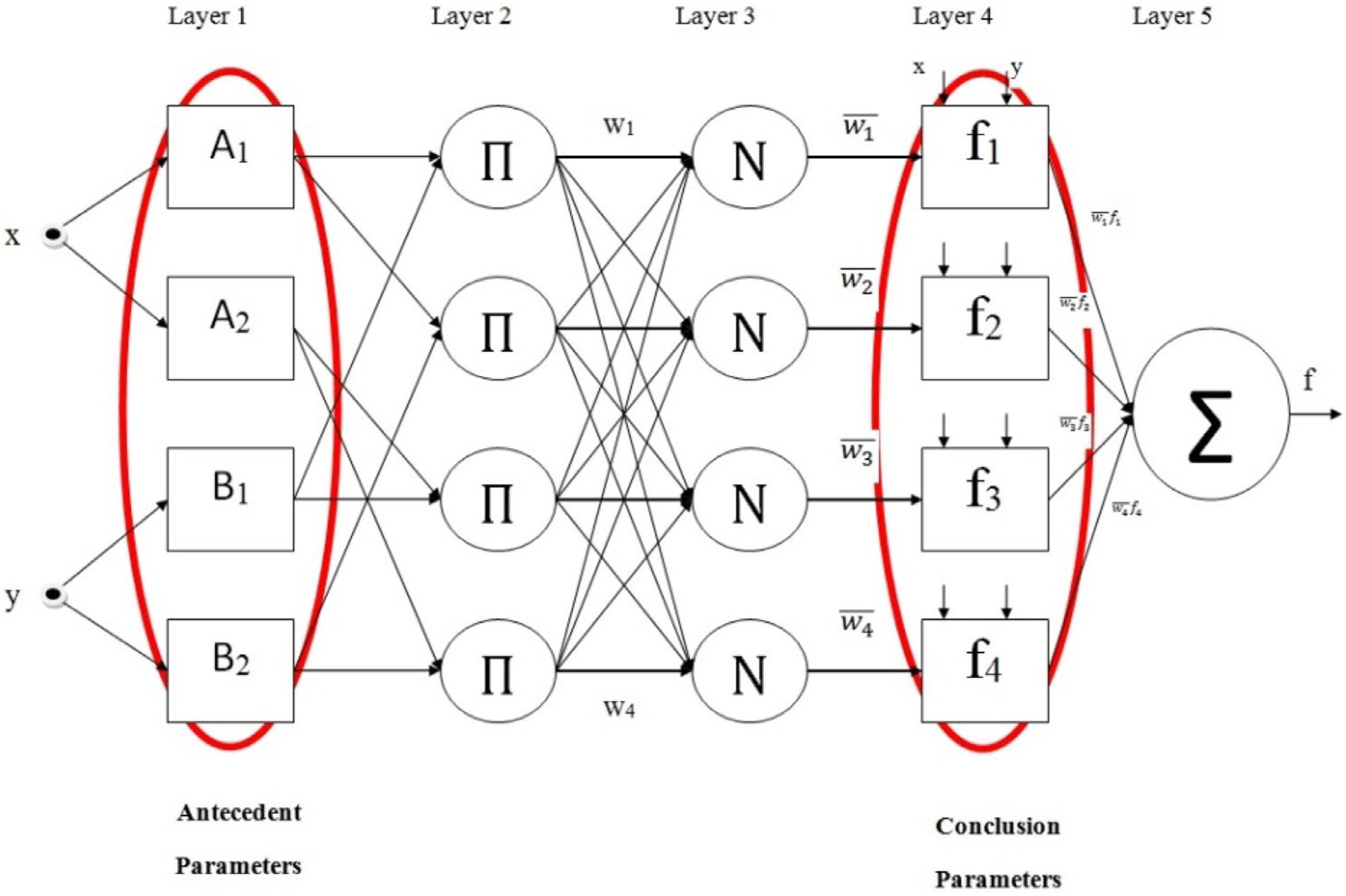
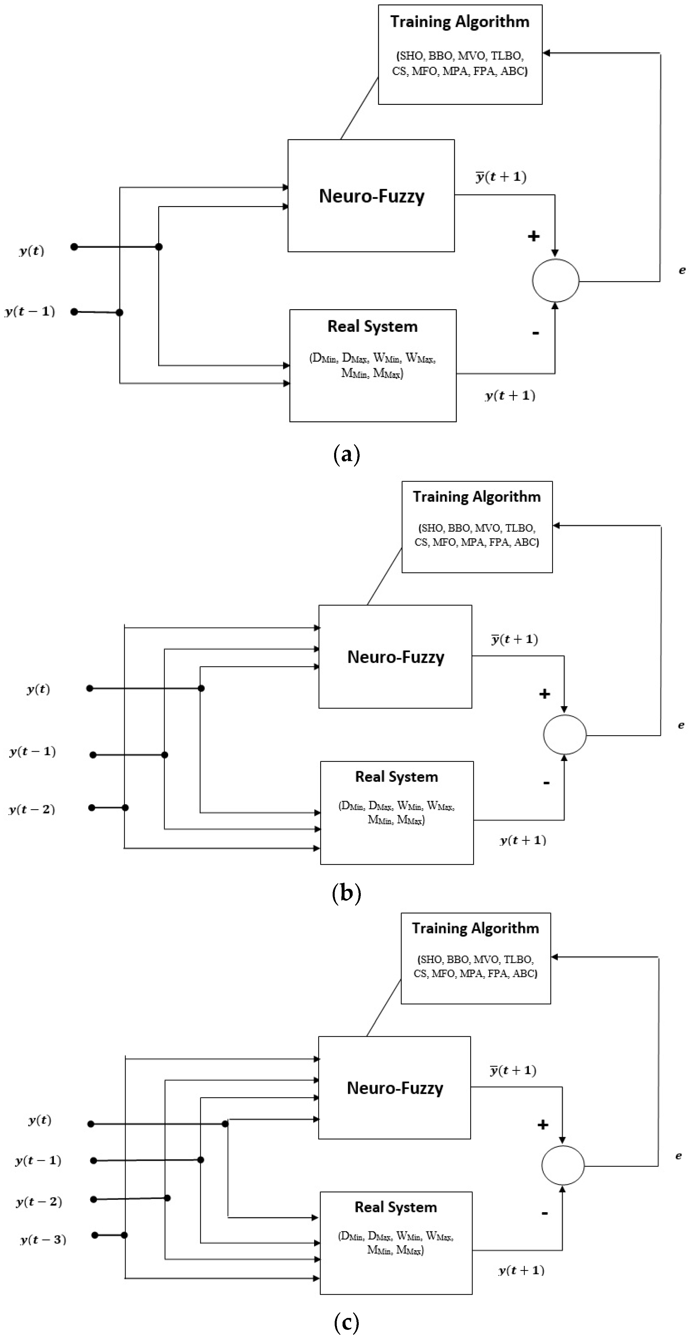
The ANFIS structures used in the study are illustrated in Figure 2. Figure 2a shows the block diagram of an ANFIS model with two inputs, while Figure 2b presents the training process and error calculation steps for a three-input model. Figure 2c displays the system structure when four inputs are used. In all these models, the output represents the subsequent time step value in the series.

In the preprocessing phase, normalization plays an important role, especially when the dataset is large or contains high variability. For this reason, all input and output values were normalized to the [0, 1] range. All results and evaluations were made based on these normalized values.

Another critical factor that influences the performance of ANFIS is the type and number of membership functions (MFs). According to the literature, generalized bell-shaped membership functions (gbellmf) are effective in modeling normalized time-series data. Therefore, gbellmf was selected in this study to remain consistent with existing studies and to avoid unnecessary experimentation.

Additionally, the number of membership functions significantly affects learning performance. In this work, systems with different input counts were trained using two, three, and four membership functions, respectively, in order to analyze their impact on prediction accuracy. Since the number of parameters to be optimized increases with more inputs, the number of MFs was adjusted accordingly. For example, in the model with four inputs, only two MFs were used to reduce the complexity of the learning process.

Notably, 80% of the obtained dataset is used in the training process, and 20% is utilized in the testing process. All error values in the study are calculated as mean squared error (MSE). To compare the results obtained with each algorithm fairly, the population size and maximum generation number were evaluated similarly. In other words, the population size and maximum generation number were set as 20 and 2500, respectively.

Table 2. Step-by-step workflow of the proposed ANFIS model.

Step	Description
1	Data Collection
2	Normalization and Feature Setup
3	ANFIS Structure Definition
4	Training and Testing
5	Evaluation Metrics

presents a summary of the overall workflow followed in this study. The process begins with data collection, where time-series data relevant to Brent oil prices are obtained. This is followed by the normalization and feature setup stage, where raw data are scaled to a uniform range and input–output pairs are prepared for model training. In the next step, the ANFIS structure is defined, including the selection of membership function types and their quantities. The model is then subjected to training and testing, allowing performance evaluation based on different configurations. Finally, the results are assessed through various evaluation metrics to determine prediction accuracy and overall model effectiveness.

4.1. Analysis for Predicting the Lowest and Highest Daily Prices of Brent Oil

The results obtained in estimating the daily minimum value of Brent oil price are presented in

Table 3. Comparison of the results obtained for the solution of the D_Min problem.

Algorithm	Number of Inputs	Number of MFs	Results
			Train			Test
			Mean	Best	Standard Deviation	Mean	Best	Standard Deviation
ABC	2	2	1.9 × 10−3	1.8 × 10−3	4.2 × 10−5	1.6 × 10−3	1.4 × 10−3	1.1 × 10−4
		3	1.9 × 10−3	1.8 × 10−3	3.5 × 10−5	1.6 × 10−3	1.5 × 10−3	1.0 × 10−4
		4	1.8 × 10−3	1.7 × 10−3	4.6 × 10−5	1.6 × 10−3	1.5 × 10−3	1.2 × 10−4
	3	2	1.9 × 10−3	1.7 × 10−3	6.3 × 10−5	1.6 × 10−3	1.4 × 10−3	1.0 × 10−4
		3	1.9 × 10−3	1.7 × 10−3	5.0 × 10−5	1.6 × 10−3	1.5 × 10−3	1.1 × 10−4
	4	2	1.9 × 10−3	1.8 × 10−3	5.4 × 10−5	1.7 × 10−3	1.5 × 10−3	1.4 × 10−4
FPA	2	2	1.9 × 10−3	1.7 × 10−3	3.5 × 10−5	1.6 × 10−3	1.5 × 10−3	9.5 × 10−5
		3	1.9 × 10−3	1.8 × 10−3	2.1 × 10−5	1.6 × 10−3	1.4 × 10−3	1.2 × 10−4
		4	1.9 × 10−3	1.8 × 10−3	2.3 × 10−5	1.6 × 10−3	1.5 × 10−3	9.0 × 10−5
	3	2	1.9 × 10−3	1.8 × 10−3	3.1 × 10−5	1.6 × 10−3	1.5 × 10−3	7.1 × 10−5
		3	1.9 × 10−3	1.8 × 10−3	4.1 × 10−5	1.6 × 10−3	1.5 × 10−3	1.1 × 10−4
	4	2	1.9 × 10−3	1.8 × 10−3	4.7 × 10−5	1.6 × 10−3	1.5 × 10−3	7.9 × 10−5
BBO	2	2	1.8 × 10−3	1.6 × 10−3	8.8 × 10−5	1.6 × 10−3	1.4 × 10−3	1.3 × 10−4
		3	1.7 × 10−3	1.6 × 10−3	6.1 × 10−5	1.7 × 10−3	1.6 × 10−3	9.9 × 10−5
		4	1.7 × 10−3	1.6 × 10−3	8.3 × 10−5	1.6 × 10−3	1.5 × 10−3	7.5 × 10−5
	3	2	1.7 × 10−3	1.6 × 10−3	5.5 × 10−5	1.6 × 10−3	1.5 × 10−3	3.1 × 10−5
		3	1.7 × 10−3	1.6 × 10−3	7.2 × 10−5	1.6 × 10−3	1.5 × 10−3	5.7 × 10−5
	4	2	1.7 × 10−3	1.5 × 10−3	1.1 × 10−4	1.6 × 10−3	1.5 × 10−3	3.9 × 10−3
MFO	2	2	1.8 × 10−3	1.7 × 10−3	7.4 × 10−5	1.6 × 10−3	1.5 × 10−3	3.9 × 10−5
		3	1.8 × 10−3	1.6 × 10−3	7.8 × 10−5	1.6 × 10−3	1.5 × 10−3	4.8 × 10−5
		4	1.8 × 10−3	1.6 × 10−3	7.8 × 10−5	1.6 × 10−3	1.5 × 10−3	5.6 × 10−5
	3	2	1.8 × 10−3	1.7 × 10−3	8.3 × 10−5	1.6 × 10−3	1.5 × 10−3	6.7 × 10−5
		3	1.8 × 10−3	1.6 × 10−3	7.5 × 10−5	1.6 × 10−3	1.5 × 10−3	6.2 × 10−5
	4	2	1.8 × 10−3	1.7 × 10−3	6.7 × 10−5	1.6 × 10−3	1.5 × 10−3	6.0 × 10−5
CS	2	2	1.8 × 10−3	1.7 × 10−3	3.8 × 10−5	1.6 × 10−3	1.5 × 10−3	1.7 × 10−4
		3	1.8 × 10−3	1.8 × 10−3	2.7 × 10−5	1.6 × 10−3	1.4 × 10−3	7.7 × 10−5
		4	1.8 × 10−3	1.8 × 10−3	2.7 × 10−5	1.6 × 10−3	1.4 × 10−3	1.1 × 10−4
	3	2	1.9 × 10−3	1.8 × 10−3	2.7 × 10−5	1.6 × 10−3	1.4 × 10−3	9.3 × 10−5
		3	1.9 × 10−3	1.8 × 10−3	2.1 × 10−5	1.6 × 10−3	1.5 × 10−3	7.6 × 10−5
	4	2	1.9 × 10−3	1.8 × 10−3	3.5 × 10−5	1.6 × 10−3	1.5 × 10−3	9.8 × 10−5
MPA	2	2	1.7 × 10−3	1.6 × 10−3	7.4 × 10−5	1.6 × 10−3	1.5 × 10−3	5.8 × 10−5
		3	1.7 × 10−3	1.6 × 10−3	8.5 × 10−5	1.6 × 10−3	1.4 × 10−3	6.6 × 10−5
		4	1.7 × 10−3	1.6 × 10−3	6.8 × 10−5	1.6 × 10−3	1.5 × 10−3	7.1 × 10−5
	3	2	1.7 × 10−3	1.6 × 10−3	8.1 × 10−5	1.6 × 10−3	1.5 × 10−3	5.6 × 10−5
		3	1.8 × 10−3	1.6 × 10−3	6.9 × 10−5	1.6 × 10−3	1.5 × 10−3	4.6 × 10−5
	4	2	1.8 × 10−3	1.6 × 10−3	6.7 × 10−5	1.6 × 10−3	1.4 × 10−3	8.6 × 10−5
MVO	2	2	1.8 × 10−3	1.7 × 10−3	5.9 × 10−5	1.6 × 10−3	1.5 × 10−3	7.0 × 10−5
		3	1.8 × 10−3	1.7 × 10−3	6.0 × 10−5	1.6 × 10−3	1.5 × 10−3	7.9 × 10−5
		4	1.8 × 10−3	1.7 × 10−3	6.4 × 10−5	1.6 × 10−3	1.5 × 10−3	4.8 × 10−5
	3	2	1.8 × 10−3	1.7 × 10−3	5.2 × 10−5	1.6 × 10−3	1.5 × 10−3	7.9 × 10−5
		3	1.8 × 10−3	1.6 × 10−3	6.0 × 10−5	1.6 × 10−3	1.4 × 10−3	7.3 × 10−5
	4	2	1.8 × 10−3	1.7 × 10−3	5.4 × 10−5	1.6 × 10−3	1.5 × 10−3	5.3 × 10−5
SHO	2	2	1.9 × 10−3	1.8 × 10−3	1.1 × 10−4	1.6 × 10−3	1.5 × 10−3	1.4 × 10−4
		3	1.9 × 10−3	1.8 × 10−3	1.1 × 10−4	1.7 × 10−3	1.5 × 10−3	1.6 × 10−4
		4	1.9 × 10−3	1.8 × 10−3	9.0 × 10−5	1.7 × 10−3	1.5 × 10−3	1.0 × 10−4
	3	2	1.9 × 10−3	1.8 × 10−3	1.3 × 10−4	1.6 × 10−3	1.4 × 10−3	1.5 × 10−4
		3	2.1 × 10−3	1.9 × 10−3	1.4 × 10−4	1.9 × 10−3	1.5 × 10−3	3.1 × 10−4
	4	2	2.6 × 10−3	1.9 × 10−3	2.0 × 10−3	2.3 × 10−3	1.4 × 10−3	2.1 × 10−3
TLBO	2	2	1.8 × 10−3	1.6 × 10−3	8.6 × 10−5	1.6 × 10−3	1.5 × 10−3	8.7 × 10−5
		3	1.8 × 10−3	1.6 × 10−3	8.8 × 10−5	1.6 × 10−3	1.5 × 10−3	2.9 × 10−4
		4	1.7 × 10−3	1.6 × 10−3	9.1 × 10−5	1.6 × 10−3	1.5 × 10−3	1.0 × 10−4
	3	2	1.8 × 10−3	1.7 × 10−3	7.4 × 10−5	1.6 × 10−3	1.5 × 10−3	6.1 × 10−5
		3	1.7 × 10−3	1.6 × 10−3	7.4 × 10−5	1.6 × 10−3	1.5 × 10−3	4.9 × 10−5
	4	2	1.8 × 10−3	1.6 × 10−3	8.8 × 10−5	1.6 × 10−3	1.5 × 10−3	5.6 × 10−5

Best results are given in bold.

. When the results obtained for all applications of all algorithms are examined, it is seen that the average training error values do not exceed the 10⁻³ level. The mean training error values were found to be in the range of 1.7 × 10⁻³ to 2.6 × 10⁻³. The best mean training error value, 1.7 × 10⁻³, was achieved with TLBO, BBO, and MPA. The worst mean training error value was found with SHO. The results of other algorithms, except SHO, are 1.9 × 10⁻³ or better. Due to the structure of the problem, increasing the number of membership functions did not clearly improve or worsen the mean training error values. Minor behavioral differences were observed between the algorithms. The best training error value was found as 1.5 × 10⁻³ on the four-input system with BBO. Low standard deviation values were achieved for the training process. Except for a few applications, the value was at the 10⁻⁵ level. The best mean test error value was found to be 1.6 × 10⁻³, and this value was obtained from many algorithms and many applications. The training algorithms could not make the mean test error value better than 1.6 × 10⁻³. In addition, the best mean training error and the best mean test error values are parallel to each other. 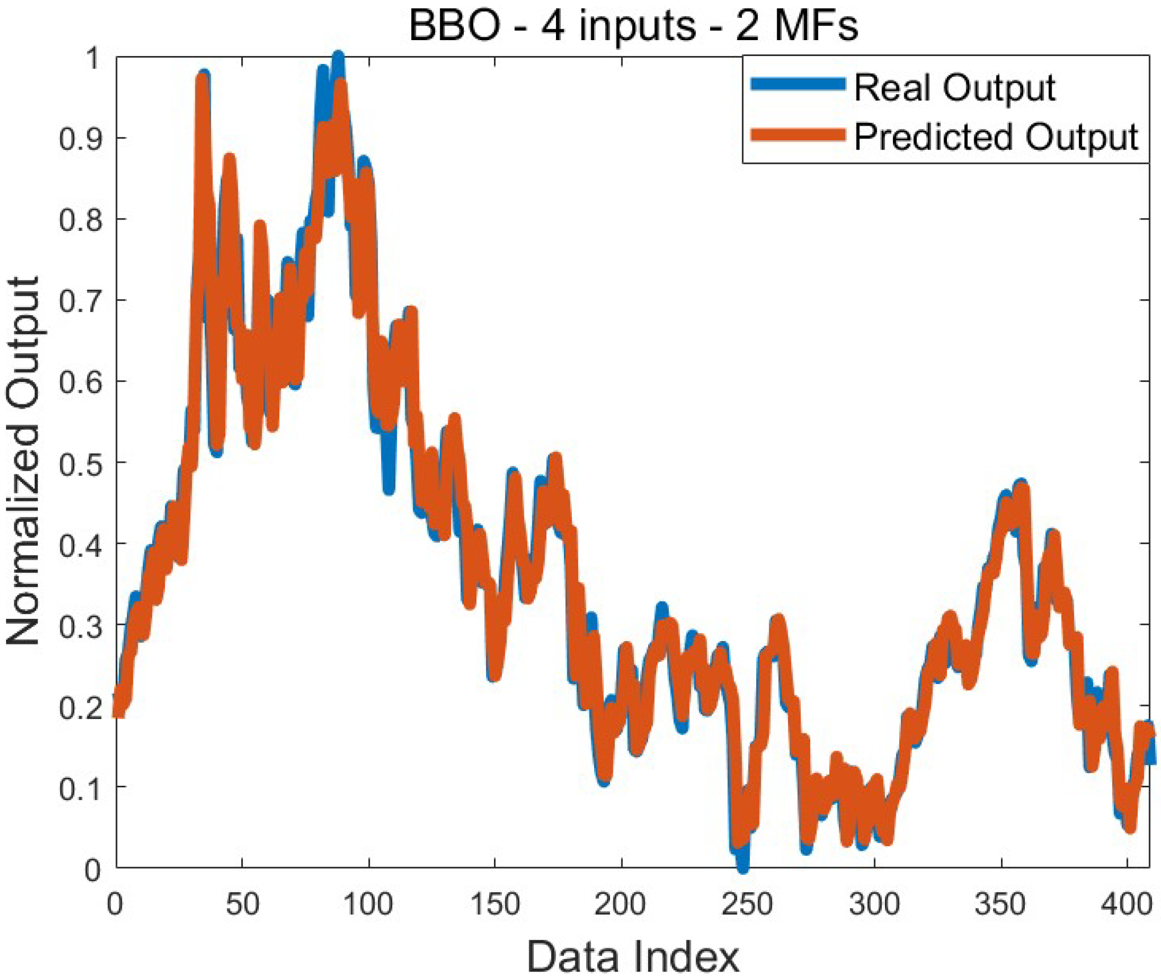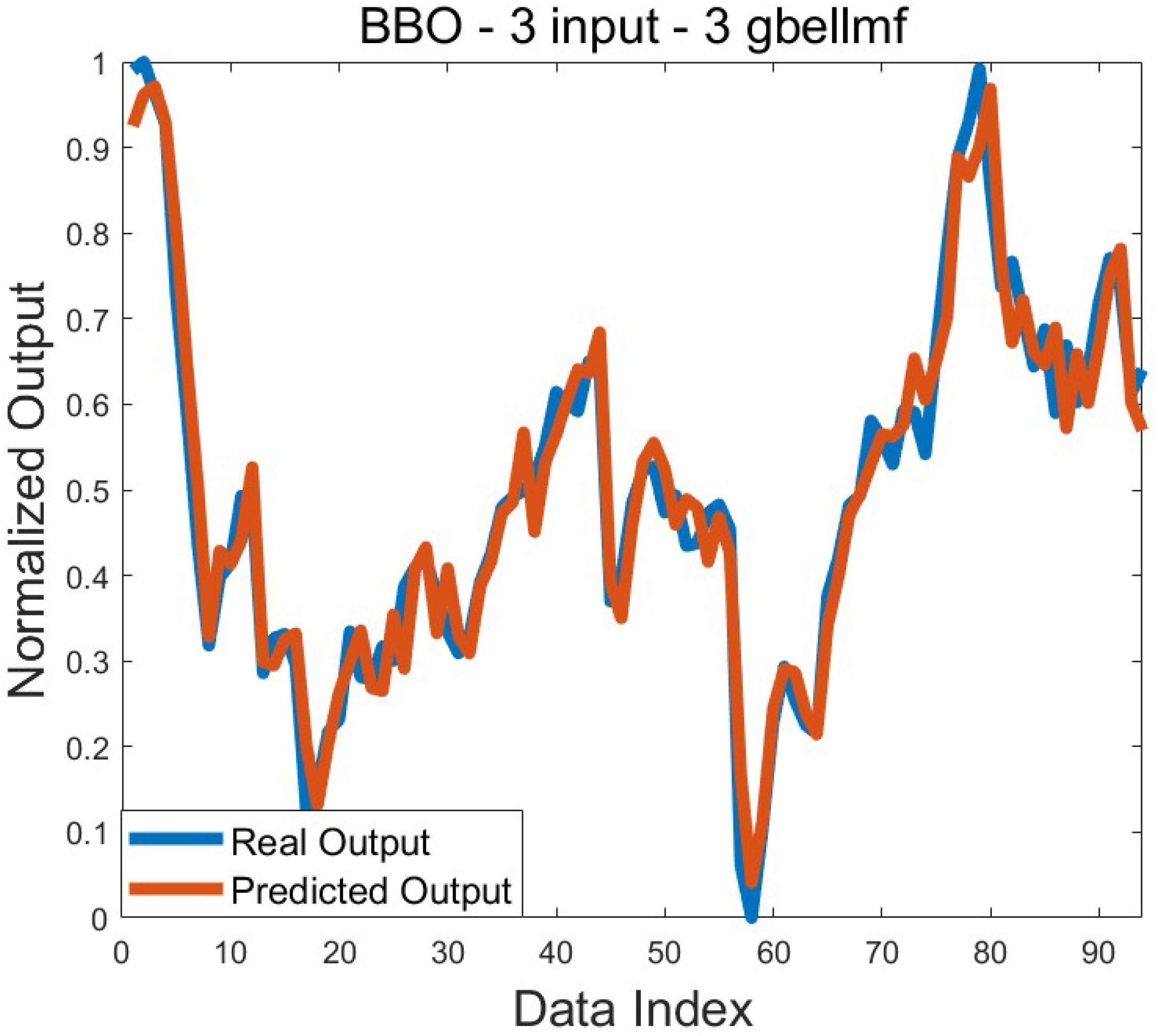The best test error value was 1.4 × 10⁻³. This value can be obtained with different algorithms. Good standard deviation values were also achieved for the test, except for a few applications. The comparison graph for the real output and the predicted output, taking into account the best training error value obtained with BBO, is presented in Figure 3.

Table 4. Comparison of the results obtained for the solution of the D_Max problem.

Algorithm	Number of Inputs	Number of MFs	Results
			Train			Test
			Mean	Best	Standard Deviation	Mean	Best	Standard Deviation
ABC	2	2	1.1 × 10−3	1.0 × 10−3	5.1 × 10−5	1.2 × 10−3	9.3 × 10−4	1.0 × 10−4
		3	1.1 × 10−3	9.3 × 10−4	5.6 × 10−5	1.1 × 10−3	9.6 × 10−4	7.1 × 10−5
		4	1.1 × 10−3	1.0 × 10−3	2.7 × 10−5	1.1 × 10−3	9.2 × 10−4	9.2 × 10−5
	3	2	1.1 × 10−3	9.5 × 10−4	6.1 × 10−5	1.1 × 10−3	8.8 × 10−4	1.1 × 10−4
		3	1.1 × 10−3	1.0 × 10−3	4.2 × 10−5	1.1 × 10−3	8.9 × 10−4	1.8 × 10−4
	4	2	1.1 × 10−3	1.0 × 10−3	4.1 × 10−5	1.1 × 10−3	1.0 × 10−3	9.1 × 10−4
FPA	2	2	1.1 × 10−3	9.9 × 10−4	3.7 × 10−5	1.2 × 10−3	1.0 × 10−3	9.5 × 10−5
		3	1.1 × 10−3	1.1 × 10−3	2.4 × 10−5	1.1 × 10−3	9.2 × 10−4	8.9 × 10−5
		4	1.1 × 10−3	1.1 × 10−3	1.7 × 10−5	1.1 × 10−3	9.4 × 10−4	8.2 × 10−5
	3	2	1.1 × 10−3	9.1 × 10−4	4.8 × 10−5	1.1 × 10−3	9.7 × 10−4	1.9 × 10−4
		3	1.2 × 10−3	1.1 × 10−3	2.3 × 10−5	1.2 × 10−3	1.0 × 10−3	1.4 × 10−4
	4	2	1.2 × 10−3	1.1 × 10−3	4.2 × 10−5	1.51 × 10−3	9.7 × 10−4	3.2 × 10−4
BBO	2	2	1.0 × 10−3	8.6 × 10−4	8.9 × 10−5	1.1 × 10−3	8.4 × 10−4	9.6 × 10−5
		3	9.5 × 10−4	8.4 × 10−4	9.9 × 10−5	1.0 × 10−3	8.9 × 10−4	8.1 × 10−5
		4	9.4 × 10−4	8.1 × 10−4	1.1 × 10−4	1.0 × 10−3	8.3 × 10−4	9.8 × 10−5
	3	2	1.1 × 10−3	8.2 × 10−4	9.1 × 10−5	1.1 × 10−3	8.8 × 10−4	1.7 × 10−4
		3	9.8 × 10−4	8.1 × 10−4	1.0 × 10−4	1.1 × 10−3	8.7 × 10−4	1.7 × 10−4
	4	2	9.6 × 10−4	8.1 × 10−4	9.7 × 10−5	1.3 × 10−3	9.8 × 10−4	2.0 × 10−4
MFO	2	2	1.1 × 10−3	8.7 × 10−4	7.1 × 10−5	1.1 × 10−3	1.0 × 10−3	5.0 × 10−5
		3	1.0 × 10−3	8.5 × 10−4	1.0 × 10−4	1.1 × 10−3	1.0 × 10−3	4.9 × 10−5
		4	1.0 × 10−3	8.1 × 10−4	1.1 × 10−4	1.1 × 10−3	9.1 × 10−4	5.7 × 10−5
	3	2	1.1 × 10−3	9.3 × 10−4	4.2 × 10−5	1.1 × 10−3	9.4 × 10−4	8.4 × 10−5
		3	1.1 × 10−3	8.5 × 10−4	6.3 × 10−5	1.0 × 10−3	9.2 × 10−4	7.3 × 10−5
	4	2	1.0 × 10−3	8.4 × 10−4	7.5 × 10−5	1.4 × 10−3	1.0 × 10−3	2.4 × 10−4
CS	2	2	1.1 × 10−3	1.0 × 10−3	2.4 × 10−5	1.4 × 10−3	9.2 × 10−4	1.0 × 10−4
		3	1.1 × 10−3	1.0 × 10−3	2.1 × 10−5	1.2 × 10−3	1.0 × 10−3	9.6 × 10−5
		4	1.1 × 10−3	1.0 × 10−3	2.5 × 10−5	1.2 × 10−3	1.0 × 10−3	1.1 × 10−4
	3	2	1.1 × 10−3	1.0 × 10−3	3.5 × 10−5	1.2 × 10−3	9.2 × 10−4	1.3 × 10−4
		3	1.1 × 10−3	1.0 × 10−3	3.1 × 10−5	1.2 × 10−3	9.6 × 10−4	2.2 × 10−4
	4	2	1.1 × 10−3	1.0 × 10−3	2.7 × 10−5	1.3 × 10−3	9.3 × 10−4	2.2 × 10−4
MPA	2	2	9.3 × 10−4	8.2 × 10−4	1.0 × 10−4	1.1 × 10−3	8.9 × 10−4	7.1 × 10−5
		3	9.7 × 10−4	8.3 × 10−4	1.1 × 10−4	1.1 × 10−3	9.2 × 10−4	7.4 × 10−5
		4	1.0 × 10−3	8.4 × 10−4	1.0 × 10−4	1.1 × 10−3	1.0 × 10−3	1.1 × 10−4
	3	2	9.8 × 10−4	8.5 × 10−4	8.9 × 10−5	1.1 × 10−3	9.7 × 10−4	7.1 × 10−5
		3	1.0 × 10−3	8.4 × 10−4	8.4 × 10−5	1.1 × 10−3	9.9 × 10−4	7.6 × 10−5
	4	2	9.8 × 10−4	8.6 × 10−4	7.1 × 10−5	1.3 × 10−3	1.0 × 10−3	2.0 × 10−4
MVO	2	2	1.1 × 10−3	9.1 × 10−4	4.8 × 10−5	1.1 × 10−3	9.9 × 10−4	5.1 × 10−5
		3	1.1 × 10−3	9.5 × 10−4	5.7 × 10−5	1.1 × 10−3	9.7 × 10−4	7.0 × 10−5
		4	1.1 × 10−3	9.7 × 10−4	4.3 × 10−5	1.1 × 10−3	9.9 × 10−4	8.2 × 10−5
	3	2	1.1 × 10−3	9.1 × 10−4	5.4 × 10−5	1.1 × 10−3	9.0 × 10−4	1.0 × 10−4
		3	1.1 × 10−3	9.2 × 10−4	5.3 × 10−5	1.1 × 10−3	9.2 × 10−4	1.2 × 10−4
	4	2	1.1 × 10−3	9.1 × 10−4	5.5 × 10−5	1.3 × 10−3	9.1 × 10−4	2.2 × 10−4
SHO	2	2	1.1 × 10−3	9.2 × 10−4	8.7 × 10−5	1.2 × 10−3	9.0 × 10−4	1.6 × 10−4
		3	1.1 × 10−3	8.8 × 10−4	1.2 × 10−4	1.2 × 10−3	8.5 × 10−4	1.6 × 10−4
		4	1.1 × 10−3	1.0 × 10−3	8.4 × 10−5	1.2 × 10−3	9.2 × 10−4	1.7 × 10−4
	3	2	1.1 × 10−3	1.0 × 10−3	5.2 × 10−5	1.3 × 10−3	9.0 × 10−4	3.6 × 10−4
		3	1.0 × 10−3	1.1 × 10−3	2.0 × 10−4	1.6 × 10−3	1.0 × 10−3	5.5 × 10−4
	4	2	1.3 × 10−3	1.0 × 10−3	1.4 × 10−4	1.6 × 10−3	9.9 × 10−4	3.3 × 10−4
TLBO	2	2	1.1 × 10−3	8.3 × 10−4	6.8 × 10−5	1.1 × 10−3	1.0 × 10−3	4.3 × 10−5
		3	1.0 × 10−3	8.5 × 10−4	1.2 × 10−4	1.1 × 10−3	9.8 × 10−4	6.3 × 10−5
		4	9.7 × 10−4	8.3 × 10−4	1.1 × 10−4	1.1 × 10−3	9.9 × 10−4	5.4 × 10−5
	3	2	1.0 × 10−3	8.2 × 10−4	1.0 × 10−4	1.1 × 10−3	9.5 × 10−4	4.2 × 10−5
		3	9.9 × 10−4	8.2 × 10−4	1.2 × 10−4	1.0 × 10−3	9.1 × 10−4	1.1 × 10−4
	4	2	9.6 × 10−4	7.7 × 10−4	8.3 × 10−5	1.4 × 10−3	9.3 × 10−4	3.1 × 10−4

Best results are given in bold.

presents a comparison of the estimates for the highest daily price of Brent oil. Changing the number of membership functions affected the results differently depending on the training algorithms. When the training results are evaluated, it is seen that the change in the number of membership functions does not change the mean error values obtained with ABC, CS, and MVO. In all applications of these algorithms, the 1.1 × 10⁻³ value was reached as the mean error value. The increase in the number of membership functions improved the mean training error in BBO and TLBO. The opposite situation was observed in MPA. The best mean training error value was obtained on a two-input system using MPA. This value is 9.3 × 10⁻⁴. After MPA, the best mean training error value belongs to BBO. The best training error value was found to be 7.7 × 10⁻⁴ on the four-input system using TLBO. For at least one implementation of algorithms other than CS, the best training errors are at a level of 10⁻⁴. Effective standard deviation values were obtained, especially because the training error values found by the algorithms were close to each other. When we look at the mean test error values, we see that the algorithms mostly obtain results that are close to each other. The mean test error values are in the range of 1.0 × 10⁻³ to 1.6 × 10⁻³. The best mean error value was found to be 1.0 × 10⁻³ with BBO, MFO, and TLBO. According to all test results, the mean error value is frequently obtained as 1.1 × 10⁻³. In fact, these results are parallel to the training results. As with the mean test error value, the best test error value also belongs to BBO. It is 8.3 × 10⁻⁴. In addition to that, effective standard deviation values were obtained in the test results. 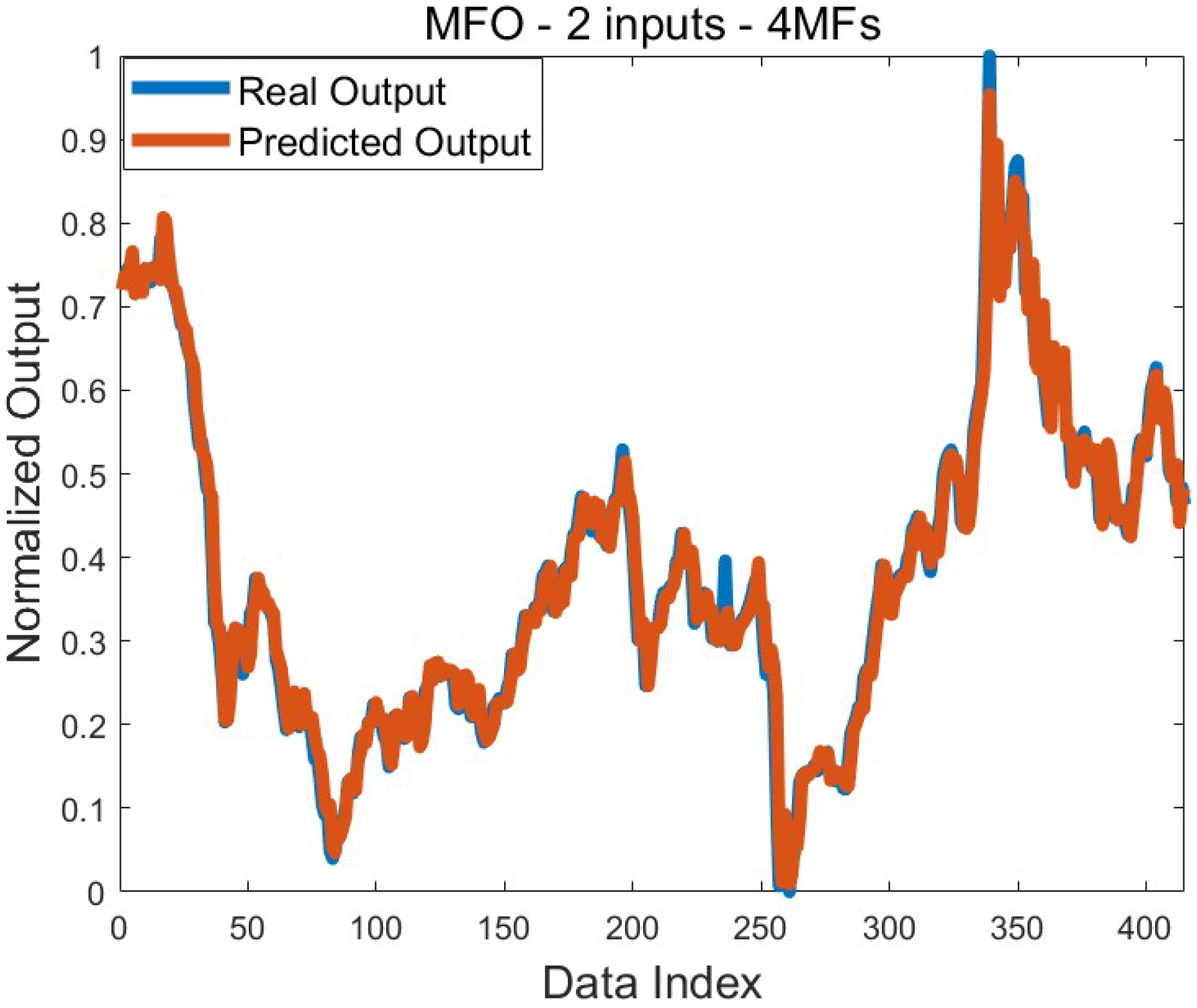Figure 4 presents the comparison of graphs of real and predicted outputs plotted according to the best training error obtained for the highest daily Brent oil price. It is seen that a very successful prediction was made, and the predicted output mostly coincides with the actual output.

4.2. Analysis for Predicting the Lowest and Highest Weekly Prices of Brent Oil

Table 5. Comparison of the results obtained for the solution of the W_Min problem.

Algorithm	Number of Inputs	Number of MFs	Results
			Train			Test
			Mean	Best	Standard Deviation	Mean	Best	Standard Deviation
ABC	2	2	7.8 × 10−4	7.2 × 10−4	3.2 × 10−5	1.1 × 10−3	9.8 × 10−4	8.0 × 10−5
		3	7.8 × 10−4	7.2 × 10−4	3.6 × 10−5	1.1 × 10−3	9.4 × 10−4	6.4 × 10−5
		4	7.8 × 10−4	7.4 × 10−4	2.2 × 10−5	1.1 × 10−3	1.0 × 10−3	6.7 × 10−5
	3	2	8.1 × 10−4	7.1 × 10−4	5.1 × 10−5	1.1 × 10−3	9.7 × 10−4	7.2 × 10−5
		3	8.2 × 10−4	7.5 × 10−4	3.8 × 10−5	1.1 × 10−3	9.9 × 10−4	7.7 × 10−5
	4	2	8.6 × 10−4	7.9 × 10−4	5.0 × 10−5	1.2 × 10−3	1.0 × 10−3	7.8 × 10−5
FPA	2	2	7.5 × 10−4	7.3 × 10−4	1.2 × 10−5	1.0 × 10−3	9.4 × 10−4	4.4 × 10−5
		3	7.7 × 10−4	7.3 × 10−4	2.1 × 10−5	1.1 × 10−3	8.7 × 10−4	7.8 × 10−5
		4	7.7 × 10−4	7.4 × 10−4	1.4 × 10−5	1.1 × 10−3	9.9 × 10−4	5.7 × 10−5
	3	2	7.9 × 10−4	7.4 × 10−4	3.0 × 10−5	1.1 × 10−3	1.0 × 10−3	6.1 × 10−5
		3	8.1 × 10−4	7.6 × 10−4	2.7 × 10−5	1.1 × 10−3	9.5 × 10−4	6.1 × 10−5
	4	2	8.4 × 10−4	7.7 × 10−4	4.4 × 10−5	1.1 × 10−3	1.0 × 10−3	8.9 × 10−5
BBO	2	2	7.2 × 10−4	7.1 × 10−4	6.8 × 10−6	1.0 × 10−3	9.7 × 10−4	2.8 × 10−5
		3	7.2 × 10−4	7.0 × 10−4	4.3 × 10−6	1.0 × 10−3	9.6 × 10−4	4.4 × 10−5
		4	7.1 × 10−4	6.6 × 10−4	1.4 × 10−5	1.0 × 10−3	9.9 × 10−4	3.0 × 10−5
	3	2	7.2 × 10−4	7.0 × 10−4	9.1 × 10−6	1.1 × 10−3	9.5 × 10−4	5.7 × 10−5
		3	7.1 × 10−4	7.0 × 10−4	7.8 × 10−6	1.1 × 10−3	9.9 × 10−4	5.0 × 10−5
	4	2	7.2 × 10−4	6.6 × 10−4	1.6 × 10−5	1.1 × 10−3	9.6 × 10−4	5.6 × 10−5
MFO	2	2	7.4 × 10−4	7.2 × 10−4	4.5 × 10−6	1.0 × 10−3	9.9 × 10−4	2.4 × 10−5
		3	7.3 × 10−4	7.2 × 10−4	4.1 × 10−6	1.0 × 10−3	9.9 × 10−4	2.2 × 10−5
		4	7.2 × 10−4	7.1 × 10−4	8.6 × 10−6	1.0 × 10−3	9.9 × 10−4	3.1 × 10−5
	3	2	7.3 × 10−4	7.0 × 10−4	9.6 × 10−6	1.0 × 10−3	9.8 × 10−4	2.1 × 10−5
		3	7.3 × 10−4	7.1 × 10−4	1.1 × 10−5	1.1 × 10−3	9.8 × 10−4	5.1 × 10−5
	4	2	7.4 × 10−4	7.2 × 10−4	1.6 × 10−5	1.1 × 10−3	1.0 × 10−3	8.7 × 10−5
CS	2	2	7.4 × 10−4	7.3 × 10−4	5.3 × 10−6	1.0 × 10−3	9.4 × 10−4	3.6 × 10−5
		3	7.4 × 10−4	7.3 × 10−4	8.4 × 10−6	1.0 × 10−3	9.6 × 10−4	4.7 × 10−5
		4	7.5 × 10−4	7.3 × 10−4	1.3 × 10−5	1.0 × 10−3	9.6 × 10−4	4.7 × 10−5
	3	2	7.6 × 10−4	7.4 × 10−4	1.5 × 10−5	1.1 × 10−3	9.7 × 10−4	9.9 × 10−5
		3	7.8 × 10−4	7.5 × 10−4	1.5 × 10−5	1.1 × 10−3	1.0 × 10−3	6.1 × 10−5
	4	2	8.0 × 10−4	7.6 × 10−4	2.7 × 10−5	1.1 × 10−3	9.9 × 10−4	7.9 × 10−5
MPA	2	2	7.2 × 10−4	7.1 × 10−4	6.2 × 10−6	1.0 × 10−3	9.9 × 10−4	1.5 × 10−5
		3	7.2 × 10−4	7.0 × 10−4	7.0 × 10−6	1.0 × 10−3	9.8 × 10−4	1.9 × 10−5
		4	7.2 × 10−4	7.1 × 10−4	5.8 × 10−6	1.0 × 10−3	9.7 × 10−4	2.3 × 10−5
	3	2	7.1 × 10−4	6.7 × 10−4	1.1 × 10−5	1.1 × 10−3	9.7 × 10−4	4.7 × 10−5
		3	7.1 × 10−4	6.8 × 10−4	1.2 × 10−5	1.1 × 10−3	9.6 × 10−4	1.3 × 10−4
	4	2	7.1 × 10−4	6.9 × 10−4	6.9 × 10−6	1.1 × 10−3	1.0 × 10−3	2.8 × 10−5
MVO	2	2	7.3 × 10−4	7.2 × 10−4	4.1 × 10−6	1.0 × 10−3	9.9 × 10−4	2.6 × 10−5
		3	7.3 × 10−4	7.2 × 10−4	5.8 × 10−6	1.0 × 10−3	9.9 × 10−4	1.9 × 10−5
		4	7.3 × 10−4	7.1 × 10−4	9.2 × 10−6	1.0 × 10−3	9.8 × 10−4	2.8 × 10−5
	3	2	7.3 × 10−4	7.1 × 10−4	9.8 × 10−6	1.1 × 10−3	9.7 × 10−4	4.3 × 10−5
		3	7.3 × 10−4	7.2 × 10−4	1.4 × 10−5	1.1 × 10−3	9.4 × 10−4	9.5 × 10−5
	4	2	7.4 × 10−4	7.2 × 10−4	2.4 × 10−5	1.1 × 10−3	9.5 × 10−4	5.5 × 10−5
SHO	2	2	7.5 × 10−4	7.2 × 10−4	3.9 × 10−5	1.1 × 10−3	9.6 × 10−4	7.0 × 10−5
		3	7.9 × 10−4	7.3 × 10−4	6.2 × 10−5	1.1 × 10−3	9.9 × 10−4	1.6 × 10−4
		4	8.1 × 10−4	7.4 × 10−4	6.3 × 10−5	1.1 × 10−3	9.9 × 10−4	9.8 × 10−5
	3	2	8.2 × 10−4	7.1 × 10−4	1.4 × 10−4	1.1 × 10−3	9.9 × 10−4	1.8 × 10−4
		3	1.0 × 10−3	7.7 × 10−4	1.8 × 10−4	1.1 × 10−3	1.0 × 10−3	2.6 × 10−4
	4	2	1.1 × 10−3	7.5 × 10−4	3.1 × 10−4	1.5 × 10−3	1.1 × 10−3	5.1 × 10−4
TLBO	2	2	7.2 × 10−4	7.0 × 10−4	8.8 × 10−6	1.0 × 10−3	9.9 × 10−4	1.6 × 10−5
		3	7.2 × 10−4	6.9 × 10−4	1.1 × 10−5	1.0 × 10−3	9.8 × 10−4	2.7 × 10−5
		4	7.2 × 10−4	6.9 × 10−4	1.2 × 10−5	1.0 × 10−3	9.7 × 10−4	2.6 × 10−5
	3	2	7.2 × 10−4	6.8 × 10−4	1.4 × 10−5	1.1 × 10−3	1.0 × 10−3	3.1 × 10−5
		3	7.1 × 10−4	6.6 × 10−4	1.5 × 10−5	1.1 × 10−3	9.9 × 10−4	4.7 × 10−5
	4	2	7.2 × 10−4	6.7 × 10−4	1.5 × 10−5	1.1 × 10−3	9.9 × 10−4	5.4 × 10−5

Best results are given in bold.

shows the results obtained with the training algorithms for predicting the lowest weekly price. Although it varies according to the training algorithms, the increase in the number of membership functions usually does not significantly affect the mean training error values. Except for a few applications of SHO, the mean training error value at a level of 10⁻⁴ was achieved. The best mean training error value was found to be 7.1 × 10⁻⁴ with BBO, MPA, and TLBO. The worst mean training error value for this problem was obtained on the four-input system using SHO. In other words, the mean training error value in all applications is in the range of 7.1 × 10⁻⁴ to 1.1 × 10⁻³. In addition, the best training error value was found to be 6.6 × 10⁻⁴ using TLBO and BBO. When we look at the training results, generally, successful results were obtained in all algorithms. It is seen that these results are supported by low standard deviation values. Standard deviations were found especially at the 10⁻⁴, 10⁻⁵, and 10⁻⁶ levels. No algorithm was able to find a better result than 1.0 × 10⁻³ in the mean test error values. In this respect, it is a fact that test error values lag behind training error values. The best mean test error was found using FPA, BBO, MFO, CS, MPA, MVO, and TLBO. The worst mean error value was reached with SHO. In other words, it is possible to say that the mean test error values were obtained in the range of 1.0 × 10⁻³ to 1.5 × 10⁻³. The best test error value was found to be 9.4 × 10⁻⁴. The effective standard deviation value was reached in the testing process as well as in the training process. 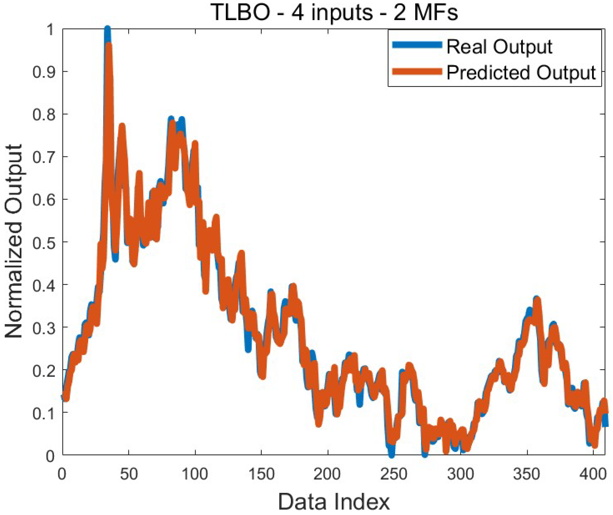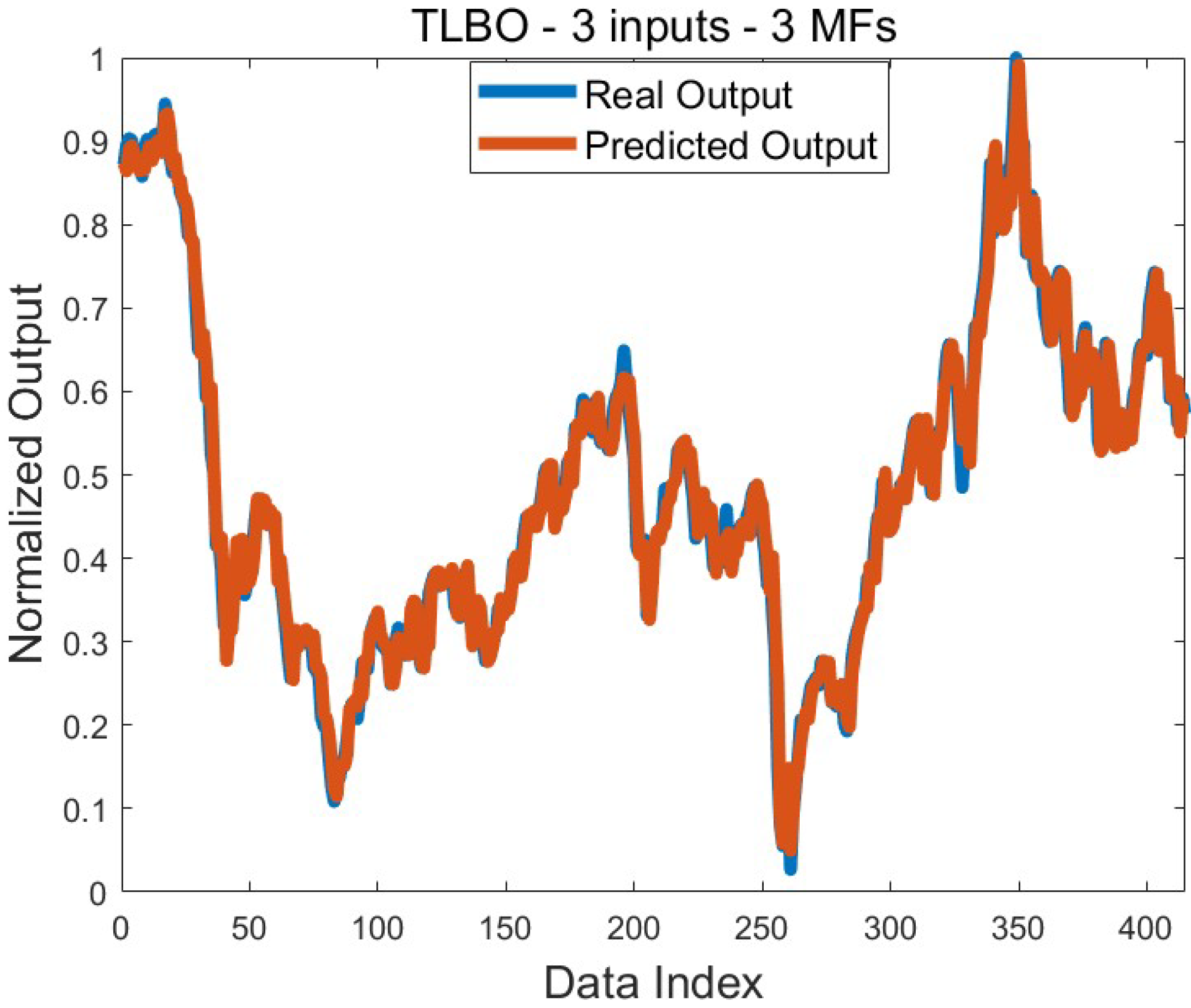Figure 5 shows the comparison graph of the predicted output and the real output for the mean error value of 7.1 × 10⁻⁴. Since this result was obtained with several algorithms, the graph was drawn by considering only the result found with TLBO. The large overlap of both graphs is an indication that the training process was successful.

Table 6. Comparison of the results obtained for the solution of the W_Max problem.

Algorithm	Number of Inputs	Number of MFs	Results
			Train			Test
			Mean	Best	Standard Deviation	Mean	Best	Standard Deviation
ABC	2	2	7.5 × 10−4	6.3 × 10−4	5.2 × 10−5	7.0 × 10−4	5.1 × 10−4	2.7 × 10−4
		3	7.4 × 10−4	6.6 × 10−4	4.2 × 10−5	7.0 × 10−4	4.7 × 10−4	1.4 × 10−4
		4	7.2 × 10−4	6.3 × 10−4	4.1 × 10−5	8.1 × 10−4	5.4 × 10−4	7.6 × 10−4
	3	2	7.8 × 10−4	6.2 × 10−4	6.4 × 10−5	7.3 × 10−4	5.0 × 10−4	2.2 × 10−4
		3	7.7 × 10−4	6.5 × 10−4	4.6 × 10−5	6.9 × 10−4	5.5 × 10−4	5.1 × 10−5
	4	2	8.2 × 10−4	7.1 × 10−4	4.8 × 10−5	6.8 × 10−4	5.2 × 10−4	1.2 × 10−4
FPA	2	2	7.2 × 10−4	6.1 × 10−4	3.8 × 10−5	6.4 × 10−4	4.7 × 10−4	1.2 × 10−4
		3	7.4 × 10−4	6.7 × 10−4	3.2 × 10−5	6.3 × 10−4	5.0 × 10−4	8.9 × 10−5
		4	7.4 × 10−4	6.8 × 10−4	3.1 × 10−5	6.1 × 10−4	5.0 × 10−4	7.8 × 10−5
	3	2	7.7 × 10−4	6.7 × 10−4	3.7 × 10−5	6.5 × 10−4	5.0 × 10−4	1.2 × 10−4
		3	8.0 × 10−4	7.1 × 10−4	3.3 × 10−5	6.3 × 10−4	5.3 × 10−4	6.9 × 10−5
	4	2	8.4 × 10−4	7.7 × 10−4	4.0 × 10−5	6.8 × 10−4	5.4 × 10−4	8.31 × 10−5
BBO	2	2	6.3 × 10−4	5.7 × 10−4	3.5 × 10−5	6.7 × 10−4	4.6 × 10−4	1.1 × 10−4
		3	6.1 × 10−4	5.5 × 10−4	3.7 × 10−5	7.4 × 10−4	4.8 × 10−4	2.3 × 10−4
		4	6.0 × 10−4	5.6 × 10−4	2.7 × 10−5	7.1 × 10−4	4.7 × 10−4	2.5 × 10−4
	3	2	6.4 × 10−4	5.5 × 10−4	5.7 × 10−5	6.9 × 10−4	5.1 × 10−4	2.1 × 10−4
		3	6.3 × 10−4	5.6 × 10−4	5.2 × 10−5	6.4 × 10−4	5.0 × 10−4	7.7 × 10−4
	4	2	6.6 × 10−4	5.6 × 10−4	6.6 × 10−5	6.6 × 10−4	4.8 × 10−4	1.6 × 10−4
MFO	2	2	7.1 × 10−4	6.1 × 10−4	9.3 × 10−5	6.7 × 10−4	5.1 × 10−4	1.1 × 10−4
		3	6.6 × 10−4	5.5 × 10−4	5.6 × 10−5	6.9 × 10−4	4.6 × 10−4	1.2 × 10−4
		4	6.4 × 10−4	5.4 × 10−4	4.6 × 10−5	6.5 × 10−4	5.1 × 10−4	9.4 × 10−5
	3	2	6.9 × 10−4	5.8 × 10−4	6.0 × 10−5	6.6 × 10−4	5.1 × 10−4	9.4 × 10−5
		3	6.6 × 10−4	6.0 × 10−4	3.9 × 10−5	6.9 × 10−4	4.8 × 10−4	2.0 × 10−4
	4	2	7.0 × 10−4	5.5 × 10−4	6.0 × 10−5	6.1 × 10−4	4.8 × 10−4	8.2 × 10−5
CS	2	2	6.6 × 10−4	6.4 × 10−4	2.7 × 10−5	6.3 × 10−4	4.8 × 10−4	1.1 × 10−4
		3	7.0 × 10−4	6.7 × 10−4	1.7 × 10−5	6.0 × 10−4	4.9 × 10−4	5.5 × 10−5
		4	7.0 × 10−4	6.7 × 10−4	2.0 × 10−5	6.0 × 10−4	5.1 × 10−4	2.6 × 10−5
	3	2	7.2 × 10−4	7.0 × 10−4	1.9 × 10−5	6.3 × 10−4	5.2 × 10−4	3.9 × 10−5
		3	7.4 × 10−4	7.0 × 10−4	3.1 × 10−5	6.4 × 10−4	5.3 × 10−4	1.6 × 10−5
	4	2	7.1 × 10−4	7.0 × 10−4	1.6 × 10−5	6.6 × 10−4	5.4 × 10−4	3.3 × 10−5
MPA	2	2	6.1 × 10−4	5.7 × 10−4	2.6 × 10−5	6.9 × 10−4	4.7 × 10−4	9.2 × 10−5
		3	6.0 × 10−4	5.7 × 10−4	2.0 × 10−5	6.5 × 10−4	4.7 × 10−4	1.2 × 10−4
		4	6.2 × 10−4	5.8 × 10−4	3.8 × 10−5	6.8 × 10−4	4.6 × 10−4	1.7 × 10−4
	3	2	6.4 × 10−4	5.8 × 10−4	4.5 × 10−5	6.4 × 10−4	5.0 × 10−4	6.4 × 10−5
		3	6.3 × 10−4	5.8 × 10−4	2.8 × 10−5	6.7 × 10−4	5.4 × 10−4	1.2 × 10−4
	4	2	6.5 × 10−4	5.7 × 10−4	5.7 × 10−5	6.3 × 10−4	5.2 × 10−4	6.1 × 10−5
MVO	2	2	6.6 × 10−4	6.0 × 10−4	4.4 × 10−5	6.8 × 10−4	5.3 × 10−4	1.1 × 10−4
		3	6.5 × 10−4	6.0 × 10−4	4.0 × 10−5	7.1 × 10−4	5.1 × 10−4	1.7 × 10−4
		4	6.5 × 10−4	6.1 × 10−4	3.9 × 10−5	6.4 × 10−4	4.9 × 10−4	1.1 × 10−4
	3	2	6.8 × 10−4	6.0 × 10−4	5.1 × 10−5	6.4 × 10−4	5.3 × 10−4	1.7 × 10−4
		3	6.8 × 10−4	6.1 × 10−4	5.0 × 10−5	6.3 × 10−4	4.7 × 10−4	8.9 × 10−5
	4	2	7.2 × 10−4	6.2 × 10−4	6.5 × 10−5	5.8 × 10−4	4.6 × 10−4	6.2 × 10−5
SHO	2	2	7.2 × 10−4	6.1 × 10−4	8.1 × 10−5	6.6 × 10−4	5.2 × 10−4	1.1 × 10−4
		3	7.5 × 10−4	6.2 × 10−4	7.8 × 10−5	6.4 × 10−4	4.7 × 10−4	7.7 × 10−5
		4	7.8 × 10−4	6.3 × 10−4	7.1 × 10−5	6.8 × 10−4	5.6 × 10−4	9.3 × 10−5
	3	2	8.6 × 10−4	6.7 × 10−4	1.8 × 10−4	7.1 × 10−4	4.9 × 10−4	2.3 × 10−4
		3	1.0 × 10−3	7.5 × 10−4	2.9 × 10−4	7.2 × 10−4	5.6 × 10−4	3.1 × 10−4
	4	2	9.5 × 10−4	6.4 × 10−4	1.7 × 10−4	8.6 × 10−4	4.9 × 10−4	2.5 × 10−4
TLBO	2	2	6.3 × 10−4	5.8 × 10−4	2.7 × 10−5	7.4 × 10−4	5.3 × 10−4	8.0 × 10−5
		3	6.1 × 10−4	5.6 × 10−4	3.3 × 10−5	7.0 × 10−4	4.8 × 10−4	1.2 × 10−4
		4	6.2 × 10−4	5.5 × 10−4	4.5 × 10−5	6.4 × 10−4	4.7 × 10−4	1.2 × 10−4
	3	2	6.3 × 10−4	5.7 × 10−4	5.1 × 10−5	7.3 × 10−4	5.1 × 10−4	8.9 × 10−5
		3	6.2 × 10−4	5.5 × 10−4	3.8 × 10−5	6.7 × 10−4	5.0 × 10−4	1.3 × 10−4
	4	2	6.6 × 10−4	5.5 × 10−4	7.1 × 10−5	5.8 × 10−4	4.8 × 10−4	6.4 × 10−5

Best results are given in bold.

shows the results obtained for predicting the highest weekly price. Increasing the number of membership functions of the inputs in ABC, BBO, and MFO also improved the solutions. Mixed behaviors were observed in other algorithms. The best mean training error was obtained by using BBO algorithms and MPAs on the two-input system. This value is 6.0 × 10⁻⁴. The worst mean training error value was found to be 1.0 × 10⁻³ with SHO. Other application results are between the best and worst mean values specified. The best training error value was found using MFO, and its value was 5.4 × 10⁻⁴. Effective standard deviation values were reached in the training process. Except for a few applications, standard deviation was found at the 10⁻⁵ level. During the testing process, especially in FPA and TLBO, increasing the number of membership functions used in the inputs improved the mean test error value. A similar situation was observed in three-input systems in ABC, BBO, and MVO. In other applications, stable behavior was not exhibited. The best mean error value was found on four-input systems with TLBO and MVO. This value is 5.8 × 10⁻⁴. In addition, the best error value was found to be 4.6 × 10⁻⁴. This value was obtained with four different training algorithms. Successful standard deviation values were achieved in the testing process as well as in the training process. It is seen that the standard deviation values obtained in all applications are in the 10⁻⁴ or 10⁻⁵ level. Figure 6 shows a comparison graph of the predicted output and the real output based on the best training result. It is seen that the graphs overlap except for a few output values. This shows that the training process carried out to solve the relevant problem was successful.

4.3. Analysis for Predicting the Lowest and Highest Monthly Prices of Brent Oil

Table 7. Comparison of the results obtained for the solution of the M_Min problem.

Algorithm	Number of Inputs	Number of MFs	Results
			Train			Test
			Mean	Best	Standard Deviation	Mean	Best	Standard Deviation
ABC	2	2	3.5×10−3	2.9 × 10−3	1.7 × 10−4	5.2 × 10−3	4.5 × 10−3	8.2 × 10−4
		3	3.4 ×10−3	2.9 × 10−3	1.6 × 10−4	5.3 × 10−3	4.4 × 10−3	6.1 × 10−4
		4	3.3 × 10−3	3.0 × 10−3	9.4 × 10−5	5.3 × 10−3	4.5 × 10−3	5.4 × 10−4
	3	2	3.5 × 10−3	3.0 × 10−3	1.5 × 10−4	5.4 × 10−3	4.3 × 10−3	9.2 × 10−4
		3	3.4 × 10−3	3.0 × 10−3	1.4 × 10−4	5.4 × 10−3	4.5 × 10−3	6.8 × 10−4
	4	2	3.4 × 10−3	3.2 × 10−3	1.1 × 10−4	5.6 × 10−3	4.5 × 10−3	6.6 × 10−4
FPA	2	2	3.5 × 10−3	3.4 × 10−3	5.5 × 10−5	4.8 × 10−3	4.5 × 10−3	2.6 × 10−4
		3	3.5 × 10−3	3.4 × 10−3	6.8 × 10−5	5.1 × 10−3	4.5 × 10−3	5.7 × 10−4
		4	3.5 × 10−3	3.3 × 10−3	7.7 × 10−5	5.0 × 10−3	4.5 × 10−3	4.9 × 10−4
	3	2	3.6 × 10−3	3.4 × 10−3	9.4 × 10−5	5.0 × 10−3	4.4 × 10−3	3.3 × 10−4
		3	3.6 × 10−3	3.4 × 10−3	1.0 × 10−4	5.3 × 10−3	4.5 × 10−3	5.3 × 10−4
	4	2	3.7 × 10−3	3.4 × 10−3	1.8 × 10−4	5.4 × 10−3	4.5 × 10−3	8.0 × 10−4
BBO	2	2	3.3 × 10−3	2.6 × 10−3	2.7 × 10−4	5.0 × 10−3	4.5 × 10−3	3.9 × 10−4
		3	3.0 × 10−3	2.2 × 10−3	3.1 × 10−4	5.2 × 10−3	4.5 × 10−3	4.0 × 10−4
		4	3.0 × 10−3	2.4 × 10−3	2.5 × 10−4	5.4 × 10−3	4.6 × 10−3	4.7 × 10−4
	3	2	3.2 × 10−3	2.5 × 10−3	2.5 × 10−4	5.1 × 10−3	4.3 × 10−3	3.8 × 10−4
		3	2.9 × 10−3	2.1 × 10−3	3.6 × 10−4	5.4 × 10−3	4.6 × 10−3	5.8 × 10−4
	4	2	3.0 × 10−3	2.4 × 10−3	2.7 × 10−4	5.2 × 10−3	4.3 × 10−3	6.8 × 10−4
MFO	2	2	3.5 × 10−3	2.7 × 10−3	2.4 × 10−4	4.8 × 10−3	4.5 × 10−3	2.7 × 10−4
		3	3.4 × 10−3	2.6 × 10−3	2.7 × 10−4	4.9 × 10−3	4.5 × 10−3	2.8 × 10−4
		4	3.3 × 10−3	2.6 × 10−3	2.4 × 10−4	5.0 × 10−3	4.5 × 10−3	3.1 × 10−4
	3	2	3.4 × 10−3	2.6 × 10−3	2.7 × 10−4	4.7 × 10−3	4.4 × 10−3	3.2 × 10−4
		3	3.2 × 10−3	2.5 × 10−3	2.6 × 10−4	5.0 × 10−3	4.4 × 10−3	4.3 × 10−4
	4	2	3.3 × 10−3	2.6 × 10−3	2.4 × 10−4	5.4 × 10−3	4.5 × 10−3	1.8 × 10−3
CS	2	2	3.5 × 10−3	3.3 × 10−3	5.2 × 10−5	5.2 × 10−3	4.5 × 10−3	1.3 × 10−3
		3	3.4 × 10−3	3.3 × 10−3	4.4 × 10−5	5.0 × 10−3	4.5 × 10−3	4.3 × 10−4
		4	3.4 × 10−3	3.3 × 10−3	5.5 × 10−5	5.2 × 10−3	4.54× 10−3	4.9 × 10−4
	3	2	3.5 × 10−3	3.4 × 10−3	5.2 × 10−5	5.1 × 10−3	4.3 × 10−3	4.8 × 10−4
		3	3.5 × 10−3	3.4 × 10−3	3.3 × 10−5	5.4 × 10−3	4.5 × 10−3	4.7 × 10−4
	4	2	3.5 × 10−3	3.4 × 10−3	8.9 × 10−5	6.3 × 10−3	4.6 × 10−3	1.7 × 10−3
MPA	2	2	3.1 × 10−3	2.5 × 10−3	3.0 × 10−4	5.0 × 10−3	4.5 × 10−3	3.5 × 10−4
		3	3.2 × 10−3	2.7 × 10−3	2.4 × 10−4	5.1 × 10−3	4.5 × 10−3	4.8 × 10−4
		4	3.1 × 10−3	2.5 × 10−3	2.4 × 10−4	5.3 × 10−3	4.5 × 10−3	5.2 × 10−4
	3	2	3.0 × 10−3	2.4 × 10−3	2.9 × 10−4	4.9 × 10−3	4.3 × 10−3	3.1 × 10−4
		3	3.1 × 10−3	2.5 × 10−3	2.7 × 10−4	5.4 × 10−3	4.5 × 10−3	5.4 × 10−4
	4	2	3.0 × 10−3	2.3 × 10−3	3.2 × 10−4	5.6 × 10−3	4.5 × 10−3	9.0 × 10−4
MVO	2	2	3.4 × 10−3	2.8 × 10−3	1.6 × 10−4	4.8 × 10−3	4.4 × 10−3	3.7 × 10−4
		3	3.4 × 10−3	3.0 × 10−3	1.3 × 10−4	5.0 × 10−3	4.6 × 10−3	3.0 × 10−4
		4	3.3 × 10−3	2.9 × 10−3	1.7 × 10−4	5.1 × 10−3	4.6 × 10−3	4.2 × 10−4
	3	2	3.4 × 10−3	2.8 × 10−3	1.8 × 10−4	4.8 × 10−3	4.4 × 10−3	2.5 × 10−4
		3	3.4 × 10−3	3.1 × 10−3	1.1 × 10−4	5.2 × 10−3	4.5 × 10−3	4.4 × 10−4
	4	2	3.3 × 10−3	3.0 × 10−3	1.4 × 10−4	5.3 × 10−3	4.5 × 10−3	6.0 × 10−4
SHO	2	2	3.5 × 10−3	3.2 × 10−3	2.5 × 10−4	4.9 × 10−3	4.5 × 10−3	3.7 × 10−4
		3	3.5 × 10−3	2.7 × 10−3	3.1×10−4	5.2 × 10−3	4.4 × 10−3	4.9 × 10−4
		4	3.7 × 10−3	3.0 × 10−3	5.5×10−4	5.5 × 10−3	4.6 × 10−3	6.4 × 10−4
	3	2	3.8 × 10−3	3.1 × 10−3	4.2×10−4	5.8 × 10−3	4.0 × 10−3	3.0 × 10−3
		3	4.2 × 10−3	3.4 × 10−3	7.9×10−4	6.0 × 10−3	4.8 × 10−3	1.0 × 10−3
	4	2	4.3 × 10−3	3.3 × 10−3	7.5×10−4	6.1 × 10−3	4.8 × 10−3	1.4 × 10−3
TLBO	2	2	3.4 × 10−3	2.7 × 10−3	1.9×10−4	4.8 × 10−3	4.5 × 10−3	2.1 × 10−4
		3	3.3 × 10−3	2.6 × 10−3	1.7×10−4	5.0 × 10−3	4.6 × 10−3	3.5 × 10−4
		4	3.1 × 10−3	2.4 × 10−3	2.8×10−4	5.2 × 10−3	4.4 × 10−3	4.4 × 10−4
	3	2	3.1 × 10−3	2.2 × 10−3	3.7×10−4	4.9 × 10−3	4.4 × 10−3	3.1 × 10−4
		3	3.1 × 10−3	2.3 × 10−3	2.8×10−4	5.3 × 10−3	4.6 × 10−3	4.0 × 10−4
	4	2	3.0 × 10−3	2.3 × 10−3	3.8×10−4	5.3 × 10−3	4.5 × 10−3	5.8 × 10−4

Best results are given in bold.

shows the results of estimating the lowest monthly price of Brent oil. According to the mean error values of the training process, the increase in the number of membership functions in ABC, BBO, MFO, and TLBO algorithms generally partially improved the results. In the FPA and some results of CS, it is seen that the increase in the number of membership functions does not affect the result. Effective results were obtained in MPA with low membership numbers. In CS, better results were obtained in two-input systems. The effect of the number of membership functions is limited. In SHO, increasing the number of membership functions worsened the mean error. The best training mean error value was found to be 2.9 × 10⁻³ with BBO. A 3.0 × 10⁻³ mean error value was achieved with MPA and TLBO algorithms. The worst mean value among all algorithms was found with SHO on the four-input system. This value is 4.3 × 10⁻³. The best training error value was found to be 2.1 × 10⁻³ with the BBO algorithm. After BBO, the best training error value belongs to TLBO. The value of TLBO is 2.2 × 10⁻³. Standard deviation values were reached at 10⁻⁴ and 10⁻⁵ levels for the training process. It is particularly noteworthy that the standard deviation values obtained in the training results of CS are at the 10⁻⁵ level. When all algorithms are considered, it is seen that average test error values are reached in the 4.7 × 10⁻³ to 6.3 × 10⁻³ range. The best mean test error value was found with MFO on a three-input system. This value is 4.7 × 10⁻³. Especially in BBO, MFO, MPA, MVO, SHO, and TLBO, it was observed that the mean test error values worsened as the number of membership functions increased. The best test error value was obtained as 4.0 × 10⁻³ using SHO. It is seen that in other algorithms, error values of 4.3 × 10⁻³, 4.4 × 10⁻³, 4.5 × 10⁻³, and 4.6 × 10⁻³ are mostly obtained. In the testing process, effective standard deviation values were generally achieved. In the test condition, standard deviation values were found at the 10−4 level except for some applications of MFO, CS, and SHO. As stated before, the best training error was obtained on BBO as 2.9 × 10⁻³. Figure 7 compares the graphs of the predicted output and the real output for this result. It is seen that the real output and the predicted output are consistent with each other except for a few points.

The results obtained regarding the estimation of the highest monthly price of Brent oil are given in

Table 8. Comparison of the results obtained for the solution of the M_Max problem.

Algorithm	Number of Inputs	Number of MFs	Results
			Train			Test
			Mean	Best	Standard Deviation	Mean	Best	Standard Deviation
ABC	2	2	2.6 × 10−3	2.2 × 10−3	1.4 × 10−4	8.6 × 10−3	6.6 × 10−3	1.1 × 10−3
		3	2.4 × 10−3	2.2 × 10−3	9.0 × 10−5	8.3 × 10−3	5.4 × 10−3	1.0 × 10−3
		4	2.3 × 10−3	2.1 × 10−3	7.08× 10−5	8.2 × 10−3	6.8 × 10−3	8.9 × 10−4
	3	2	2.5 × 10−3	2.2 × 10−3	1.5 × 10−4	8.4 × 10−3	5.2 × 10−3	1.3 × 10−3
		3	2.3 × 10−3	2.1 × 10−3	1.1 × 10−4	8.4 × 10−3	6.0 × 10−3	1.2 × 10−3
	4	2	2.4 × 10−3	2.0 × 10−3	1.5 × 10−4	8.2 × 10−3	5.6 × 10−3	1.4 × 10−3
FPA	2	2	2.6 × 10−3	2.3 × 10−3	1.1 × 10−4	8.1 × 10−3	7.0 × 10−3	7.8 × 10−4
		3	2.6 × 10−3	2.4 × 10−3	8.6 × 10−5	8.3 × 10−3	7.0 × 10−3	1.0 × 10−3
		4	2.5 × 10−3	2.4 × 10−3	7.4 × 10−5	8.2 × 10−3	6.6 × 10−3	7.0 × 10−4
	3	2	2.7 × 10−3	2.4 × 10−3	9.2 × 10−5	8.0 × 10−3	6.4 × 10−3	8.9 × 10−4
		3	2.6 × 10−3	2.4 × 10−3	1.1 × 10−4	8.3 × 10−3	5.8 × 10−3	1.1 × 10−3
	4	2	2.8 × 10−3	2.4 × 10−3	1.9 × 10−4	8.5 × 10−3	5.9 × 10−3	1.5 × 10−3
BBO	2	2	2.3 × 10−3	2.0 × 10−3	1.5 × 10−4	7.7 × 10−3	5.5 × 10−3	9.4 × 10−4
		3	2.2 × 10−3	2.0 × 10−3	1.4 × 10−4	7.7 × 10−3	6.2 × 10−3	9.4 × 10−4
		4	2.1 × 10−3	2.0 × 10−3	1.2 × 10−4	7.9 × 10−3	6.2 × 10−3	1.1 × 10−3
	3	2	2.2 × 10−3	1.9 × 10−3	1.8 × 10−4	8.7 × 10−3	6.6 × 10−3	1.1 × 10−3
		3	2.0 × 10−3	1.7 × 10−3	1.7 × 10−4	8.8 × 10−3	5.9 × 10−3	2.7 × 10−3
	4	2	2.2 × 10−3	1.9 × 10−3	2.0 × 10−4	8.1 × 10−3	6.2 × 10−3	1.4 × 10−3
MFO	2	2	2.5 × 10−3	2.1 × 10−3	2.5 × 10−4	7.5 × 10−3	6.1 × 10−3	6.9 × 10−4
		3	2.4 × 10−3	2.0 × 10−3	2.1 × 10−4	7.8 × 10−3	6.4 × 10−3	7.5 × 10−4
		4	2.3 × 10−3	2.1 × 10−3	1.6 × 10−4	7.5 × 10−3	6.4 × 10−3	7.2 × 10−4
	3	2	2.5 × 10−3	2.1 × 10−3	2.2 × 10−4	8.2 × 10−3	6.5 × 10−3	7.9 × 10−4
		3	2.4 × 10−3	2.0 × 10−3	1.8 × 10−4	8.3 × 10−3	6.5 × 10−3	7.4 × 10−4
	4	2	2.4 × 10−3	2.1 × 10−3	2.3 × 10−4	8.2 × 10−3	4.9 × 10−3	1.1 × 10−3
CS	2	2	2.5 × 10−3	2.4 × 10−3	7.4 × 10−5	7.9 × 10−3	6.5 × 10−3	7.1 × 10−4
		3	2.5 × 10−3	2.4 × 10−3	6.7 × 10−5	7.8 × 10−3	5.6 × 10−3	9.2 × 10−4
		4	2.5 × 10−3	2.4 × 10−3	4.2 × 10−5	8.1 × 10−3	6.1 × 10−3	1.0 × 10−3
	3	2	2.6 × 10−3	2.4 × 10−3	8.7 × 10−5	8.8 × 10−3	6.4 × 10−3	2.5 × 10−3
		3	2.5 × 10−3	2.3 × 10−3	1.0 × 10−4	8.5 × 10−3	6.2 × 10−3	1.3 × 10−3
	4	2	2.7 × 10−3	2.5 × 10−3	1.2 × 10−4	8.1 × 10−3	5.6 × 10−3	1.3 × 10−3
MPA	2	2	2.3 × 10−3	2.1 × 10−3	9.3 × 10−5	7.8 × 10−3	6.2 × 10−3	9.4 × 10−4
		3	2.2 × 10−3	2.1 × 10−3	9.7 × 10−5	8.3 × 10−3	5.9 × 10−3	1.1 × 10−3
		4	2.2 × 10−3	2.0 × 10−3	1.1 × 10−4	8.0 × 10−3	6.0 × 10−3	9.5 × 10−4
	3	2	2.2 × 10−3	1.9 × 10−3	1.4 × 10−4	8.4 × 10−3	6.5 × 10−3	1.4 × 10−3
		3	2.2 × 10−3	1.9 × 10−3	1.3 × 10−4	8.6 × 10−3	6.4 × 10−3	9.0 × 10−4
	4	2	2.2 × 10−3	1.9 × 10−3	2.1 × 10−4	9.0 × 10−3	6.4 × 10−3	1.3 × 10−3
MVO	2	2	2.5 × 10−3	2.2 × 10−3	1.8 × 10−4	7.5 × 10−3	6.2 × 10−3	7.7 × 10−4
		3	2.4 × 10−3	2.2 × 10−3	1.1 × 10−4	7.8 × 10−3	5.8 × 10−3	8.9 × 10−4
		4	2.4 × 10−3	2.2 × 10−3	1.2 × 10−4	8.2 × 10−3	6.1 × 10−3	9.4 × 10−4
	3	2	2.5 × 10−3	2.1 × 10−3	2.0 × 10−4	8.0 × 10−3	6.1 × 10−3	9.1 × 10−4
		3	2.4 × 10−3	2.2 × 10−3	1.4 × 10−4	8.7 × 10−3	6.1 × 10−3	2.7 × 10−3
	4	2	2.5 × 10−3	2.1 × 10−3	2.8 × 10−4	7.8 × 10−3	5.7 × 10−3	1.3 × 10−3
SHO	2	2	2.7 × 10−3	2.3 × 10−3	2.4 × 10−4	8.2 × 10−3	6.1 × 10−3	8.8 × 10−4
		3	2.6 × 10−3	2.1 × 10−3	3.9 × 10−4	8.9 × 10−3	7.1 × 10−3	1.3 × 10−3
		4	2.7 × 10−3	2.1 × 10−3	3.7 × 10−4	8.6 × 10−3	6.4 × 10−3	1.1 × 10−3
	3	2	2.9 × 10−3	2.2 × 10−3	4.9 × 10−4	8.5 × 10−3	5.9 × 10−3	1.5 × 10−3
		3	3.1 × 10−3	2.4 × 10−3	4.8 × 10−4	9.0 × 10−3	7.4 × 10−3	1.2 × 10−3
	4	2	3.1 × 10−3	2.3 × 10−3	4.1 × 10−4	8.6 × 10−3	5.9 × 10−3	2.3 × 10−3
TLBO	2	2	2.4 × 10−3	2.0 × 10−3	1.6 × 10−4	8.0 × 10−3	6.5 × 10−3	1.1 × 10−3
		3	2.3 × 10−3	1.9 × 10−3	1.6 × 10−4	8.0 × 10−3	5.7 × 10−3	1.3 × 10−3
		4	2.2 × 10−3	1.8 × 10−3	1.5 × 10−4	7.9 × 10−3	6.3 × 10−3	7.7 × 10−4
	3	2	2.3 × 10−3	2.0 × 10−3	1.8 × 10−4	8.3 × 10−3	6.7 × 10−3	9.3 × 10−4
		3	2.0 × 10−3	1.6 × 10−3	2.0 × 10−4	9.2 × 10−3	7.5 × 10−3	1.1 × 10−3
	4	2	2.1 × 10−3	1.6 × 10−3	2.4 × 10−4	8.9 × 10−3	6.0 × 10−3	1.4 × 10−3

Best results are given in bold.

. The increase in the number of membership functions, especially in ABC, BBO, MFO, and TLBO, improved the training mean errors. A similar situation was observed in MVO, except for one application. All mean error values are the same except for when using two gbellmf on a two-input system, which produced a different mean training error value of the MPA. The best mean error value among all applications was found using three gbellmf on a three-input system with BBO and TLBO algorithms. This value is 2.0 × 10⁻³. Apart from BBO and TLBO, the best mean training error value belongs to MPA. The worst mean training error value belongs to SHO. This value is 3.1 × 10⁻³. In the light of this information, it is seen that the mean error values obtained for the training process in estimating the monthly maximum value are between 2.0 × 10⁻³ and 3.1 × 10⁻³. It has also been determined that the training mean errors in two- and three-input systems are generally better than in four-input systems, and the best mean training results are obtained in these systems. The best training error value was found to be 1.6 × 10⁻³ using TLBO. The best training error values found with BBO and MPA are 1.7 × 10⁻³ and 1.9 × 10⁻³, respectively. Effective standard deviation values for the training process were reached. Standard deviation values at the 10⁻⁴ or 10⁻⁵ level were obtained. Looking at the test results, the change in the number of memberships generally affected the results differently. It was observed that the mean test error values of BBO and TLBO were not as good as the mean training error values. The best test mean error values were obtained to be 7.5 × 10⁻³ using MFO and MVO. The best test error value was found to be 4.9 × 10⁻³ with MFO. The test results show that standard deviation values were obtained at 10⁻³ and 10⁻⁴ levels. These values are consistent with the results obtained. 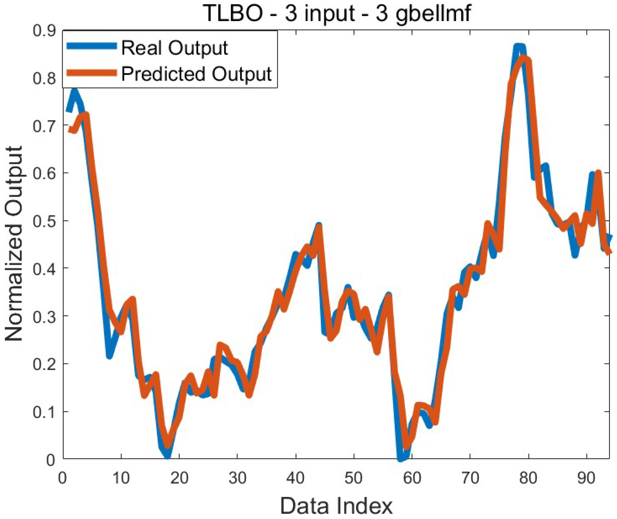Figure 8 shows the comparison of the real output and the predicted output for the best training error value. Both graphs largely overlap. This is one of the indicators demonstrating that the training process was successful.

The findings obtained in this study should be interpreted within the scope of certain limitations. In particular, the number of inputs, the number and type of membership functions, population size, and the maximum number of generations are the primary constraints considered. Exploring alternative configurations beyond these parameters may lead to higher-quality solutions. However, due to the significant time and computational cost required for such evaluations, the scope of the study was intentionally limited.

The use of historical data proved to be more effective in daily and weekly forecasts. The results clearly show that daily and weekly predictions outperform monthly predictions, as demonstrated in the related tables and figures. One possible reason for this difference is the limited number of data points in the monthly dataset. Additionally, the longer time gap between the input data and the predicted output in monthly forecasts increases the likelihood of external factors influencing the outcome, which may also reduce accuracy.

When examining both training and test results for daily, weekly, and monthly predictions, it is observed that standard deviation values are generally low. This indicates that the successful outcomes obtained are consistent and repeatable. The fact that test results largely aligned with training results suggests that the training process was effectively conducted and that no overfitting occurred.

Although all algorithms yielded effective results, it can be stated that BBO and TLBO performed better than the others in solving the target problem. This does not imply that the other algorithms were unsuccessful, but rather that these two algorithms were more suitable for this specific problem and configuration. It should also be considered that the observed performance differences may be influenced by the previously mentioned limitations of the study.

Furthermore, an increase in the number of inputs and membership functions also increases the number of parameters to be optimized during training, which extends the overall training time. Considering that each algorithm was executed 30 times for statistical validity, the increase in training duration should be considered a critical factor.

In addition to the findings discussed above, the study was conducted within a methodologically symmetric framework. Each of the nine metaheuristic algorithms was applied under identical conditions, using the same datasets, ANFIS configurations, and performance metrics. The number of runs, input–output structures, and evaluation criteria were all uniformly defined across algorithms and prediction types (daily, weekly, and monthly). This symmetric design ensured a fair comparison and enhanced the reproducibility and objectivity of the results. Such a balanced experimental structure not only strengthens the internal validity of the study but also aligns with the scientific focus of symmetry, where consistency and structured modeling approaches are emphasized.

These findings offer valuable insights into the energy market, particularly in the context of crude oil price forecasting. The results indicate that accurate short- and medium-term predictions can be achieved using ANFIS models trained with metaheuristic algorithms. The superior performance observed in daily and weekly forecasts, compared to monthly ones, highlights the potential of the proposed approach for short-term decision-making processes such as risk management, investment planning, and dynamic pricing strategies. Moreover, the consistently low standard deviation values observed across multiple runs suggest that the model is stable and reliable, which is essential for supporting data-driven decisions in volatile energy markets like crude oil trading.

5. Conclusions

In this study, an Adaptive Neuro-Fuzzy Inference System (ANFIS) was trained using nine different metaheuristic algorithms—namely SHO, BBO, MVO, TLBO, CS, MFO, MPA, FPA, and ABC—to predict short- and medium-term Brent crude oil prices. The main objective was to evaluate the performance of these training algorithms in estimating the daily, weekly, and monthly minimum and maximum price levels of Brent oil. The raw time-series data were preprocessed and transformed into ANFIS-compatible input–output structures, allowing the use of past values to predict future ones. In addition, the effects of different input sizes and varying numbers of membership functions were also systematically examined. The key findings of the study can be summarized as follows:

• All nine metaheuristic algorithms produced effective results when used to train ANFIS models for Brent oil price prediction. These findings confirm that ANFIS models enhanced with metaheuristic optimization are suitable tools for handling nonlinear and dynamic characteristics in energy market forecasting.
• A strong consistency was observed between training and test results, indicating that the models were not overfitted and maintained generalizability across different problem sets. This also highlights the robustness of the training process and the reliability of the optimized ANFIS configurations.
• Distinct mean error values were observed for daily, weekly, and monthly predictions. While some algorithms performed well in daily or weekly predictions, their effectiveness declined in monthly contexts. This observation emphasizes the need for context-specific tuning of algorithms depending on the prediction window.
• The number and type of membership functions significantly influenced the prediction performance in some cases, while in others, variations in membership function count had a negligible impact. This suggests that for certain complex problem structures, the optimization process may reach saturation, preventing further improvement regardless of parameter adjustments. Such limitations might stem from the intrinsic difficulty of the problem or insufficient input diversity.
• Across all experiments, both training and testing phases yielded low standard deviation values. This indicates that the algorithms provided stable and repeatable solutions even though each training phase started from random initial conditions. This reinforces the statistical reliability of the proposed approach.
• Although all algorithms achieved acceptable performance levels, BBO and TLBO consistently outperformed the others in most scenarios. These two algorithms demonstrated stronger optimization capabilities in guiding ANFIS training toward more accurate predictions, especially in terms of lower error rates and faster convergence.
• The symmetric structure of the evaluation process—equal iterations, consistent datasets, and identical parameter settings—strengthens the objectivity and reliability of the findings.

Overall, this study provides evidence that combining ANFIS with metaheuristic optimization offers a powerful framework for short- and medium-term energy price forecasting. The models developed here are particularly useful for stakeholders in the energy market who require reliable, interpretable, and adaptable prediction tools. These results are not only relevant in the context of Brent oil price forecasting but also offer broader insights into the use of adaptive hybrid AI systems in energy economics. The methodology demonstrated here can be adapted to other commodities and financial markets where nonlinear patterns dominate, and high prediction reliability is required. Future research may focus on exploring hybrid training strategies, incorporating additional economic indicators, or evaluating the models under real-time constraints to enhance practical applicability.