Modeling Academic Social Networks Using Covering and Matching in Intuitionistic Fuzzy Influence Graphs

Abstract

Influence graphs are essential tools for analyzing interactions and relationships in social networks. However, real-world networks often involve uncertainty due to incomplete, vague, or dynamic information. The structure of influence graphs often exhibits natural symmetries, which play a crucial role in optimizing covering and matching strategies by decreasing redundancy and enhancing efficiency. Traditional influence graph models struggle to address such complexities. To address this gap, we present the novel concepts of covering and matching in intuitionistic fuzzy influence graphs (IFIGs) for modeling academic social networks. These graphs incorporate degrees of membership and non-membership to better reflect uncertainty in influence patterns. Thus, the main aim of this study is to initiate the concepts of covering and matching within the IFIG paradigm and provide its application in social networks. Initially, we establish some basic terms related to covering and matching with illustrative examples. We also investigate complete and complete bipartite IFIGs. To verify the practicality of this study, student interactions across subjects are analyzed using strong paths and strong independent sets. The proposed model is then evaluated using the TOPSIS method to rank participants based on their influence. Moreover, a comparative study is conducted to demonstrate that the proposed model not only handles uncertainty effectively but also performs better than the existing approaches.

1. Introduction

1.1. Literature Review

In 1965, Zadeh initiated the concepts of fuzzy sets (FSs) [1], which have become a useful tool for handling uncertainty. FSs assign membership values (MVs) to each entity of an underlying set X, making it more flexible. Due to its flexible nature, a number of generalizations of FSs have been explored in the literature. In this context, IVFSs were the first extension of FSs initiated in [2]. They are unlike FSs, where MVs are single numbers from the unit interval [0, 1]. IVFSs consider MVs as subintervals of [0, 1], thereby providing a broader representation of uncertainty. However, FSs only provide information about MVs and do not account for non-membership values (NMVs). To address this limitation, Atanassov introduced the idea of IFSs in [3], which incorporate both the MVs and NMVs with the condition that their sum must lie in [0, 1]. IFSs are an important generalization of FSs and are more applicable than FSs as they include an additional value, i.e., NMV, for each element in a set X. Currently, IFSs have gained significant attention in various fields, and numerous studies have been conducted in this domain. IF-matrices with applications have been described in [4]. K Suayngam [5] added some new results by utilizing IFSs in the domain of IUP algebras. IFSs are more capable of representing uncertainty in real-world problems. An extended framework for IFSs has been described in [6]. J Mahanta presented some similarity measure for IFSs along with their application to face recognition [7]. L Zhang developed a decision-making algorithm on IFSs in [8].

Rosenfield introduced the idea of FGs in [9]. Following this, many generalizations of FGs, such as FTGs [10], BPFGs [11], and fuzzy threshold graphs [12], have been introduced. Similarly, the term IFG was presented in [13]. Few new operations on IFGs were investigated in [14]. Some new terms related to dominations in IFGs have been introduced in [15]. Sequentially, the notions of covering and domination in IFGs were investigated in [16]. Domination in intuitionistic fuzzy directed graph was described in [17]. Recently, numerous studies have been conducted on IFGs, and their applications in many fields have been explored.

On the other hand, an influence graph is a graphical model useful to describe and analyze the relationships among entities where the influence plays a role. Moreover, the structure of influence graphs often exhibits natural symmetries, which play a crucial role in optimizing covering and matching strategies by decreasing redundancy and enhancing efficiency. Numerous studies have been conducted on influence graphs, exploring different types of influence graphs and their applications across multiple fields [18,19]. However, when the influence relationships are uncertain or imprecise, fuzzy influence graphs (FIGs) provide a more flexible representation instead. Mathew et al. [20] described the concepts of FIGs and explored its application in human trafficking. Moreover, FIGs provide the effect of each node or edge in the network. The concepts of intuitionistic fuzzy incident graphs are discussed in [21]. Similarly, bipolar picture fuzzy influence graphs are described in [22]. Rehman et al. [23] introduced the concept of dominations in IFIGs. Manjusha introduced the concepts of covering, matching, and domination in FGs in [24]. These concepts in the paradigm of IFGs were initiated in [16]. The concepts of dominations in intuitionistic fuzzy directed graphs were explored in [25]. Similarly, these concepts were also addressed in the domain of PFGs [26]. Moreover, these ideas were further investigated in the domain of IVIFGs [27,28]. Some studies are concerned about interval valued fuzzy graphs and analysis of the decision making of domains, such as socioeconomic conditions and big data  [29,30,31]. Overall, the concepts of covering and matching have drawn significant attention from researchers. Furthermore,

Table 1. Generalization of FGs.

Authors	Reference	Notion Introduced
Rosenfield	[9]	Fuzzy graph
Parvathi	[13]	Intuitionistic fuzzy graph
S. Mathew	[20]	Fuzzy influence graph
Fahad ur Rehman	[23]	Intuitionistic fuzzy influence graph

, Figure 1, and

Table 2. Covering and matching in different structures.

Authors	Reference	Notion Introduced
Manjusha	[24]	Covering, matching, and paired domination in FG through SAs
Sahoo et al.	[16]	Covering and matching in IFG through SAs
Qiang, Xiaoli	[27]	Covering, matching, and paired domination in IVIFG
Jan, Naeem, et al.	[26]	Covering, matching, and paired domination in PFG

together illustrate the significance of studying the concepts of covering and matching in the domain of IFIG. The abbreviations used in this article are listed in

Table 3. Abbreviations used in this article.

Symbols	Description	Symbols	Description
FS	Fuzzy set	FG	Fuzzy graph
IFS	Intuitionistic fuzzy set	IFG	Intuitionistic fuzzy graph
BPFS	Bipolar fuzzy set	BPFG	Bipolar fuzzy graph
FTG	Fuzzy tolerance graph	FIG	Fuzzy influence graph
SC	Strong cover	IP	Influence pair
SI	Strongly independent	SIS	Strong independent set
PSM	Perfect strong matching	SM	Strong matching
SNC	Strong node cover	SPC	Strong path cover
MV	Membership value	NMV	Non-membership value
PFG	Picture fuzzy graph	NV	Neutral value
SPC number	Strong path cover number	FW	Fuzzy weight
SP	Strong path	SA	Strong arc
SPC	Strong path cover	SAC	Strong arc cover
IVFS	Interval valued fuzzy set	PM	Perfect matching
SAC number	Strong arc covering number	SNC Number	Strong node covering number
SAI number	Strong arc independent number	SIFIPC	Strong intuitionistic fuzzy influence path cover
$\overline{IP}$	Influence path	SIP	Strong influence path
IFIP	Intuitionistic fuzzy influence pair	EIP	Effective influence pair
SIFIP	Strong intuitionistic fuzzy influence pair	WIFIP	Weak intuitionistic fuzzy influence pair
SGIFIP	Strongest intuitionistic fuzzy influence pair	SIFINC	Strong intuitionistic fuzzy influence node cover
$\overline{IFIP}$	Intuitionistic fuzzy influence path

.

1.2. Motivation

FGs and IFGs analyze only the relationships between entities, but they do not explicitly capture influence between them. However, IFIGs take into account both the relationships between entities and their mutual influences. Because to this, IFIGs are more effective in modeling real-life problems with uncertainties. On the other hand, the concepts of covering and matching are fundamental terms in graph theory, which are useful for analyzing optimal selections of edges and vertices in a given graph. In this study, we extend the terms covering and matching in the domain of IFIGs. Due to the inherited properties of IFIGs, these concepts in the paradigm of IFIGs become more powerful compared with FGs and IFGs. In this study, we first initiate the concepts of covering in IFIGs and provide the characterizations of various types of IFIGs, including complete IFIGs and complete bipartite IFIGs. Subsequently, we discuss the notions of terms like SM and PSM and provide some useful results related to them. To show the effectiveness of our study, we propose a model based on our newly established concepts to manipulate the interactions among participants in social networks engaged in studying different subjects. Additionally, the proposed model is investigated through the TOPSIS method. A comparative study is also provided to prove the efficiency of our proposed model. IFIGs’ structures are more flexible and have a broader scope due to their MVs, NMVs, and influence values. Thus, the concepts of covering and matching within the domain of IFIGs would be more useful for modeling real-life problems involving uncertainties. Moreover, the notions of covering and matching have been described in FGs [24] and IFGs [16] but have not been described in IFIGs yet. All of these have motivated us to extend the concepts of covering and matching in the paradigm of IFIGs.

1.3. Novelty

The novelty of our work can be described as follows:

• The concepts of SNC, SPC, SPC number, and SIS depend on SPs in IFIGs introduced in the beginning.
• We introduce and characterize some special IFIGs, such as complete IFIGs, bipartite and IFIGs.
• The term matching and its different types, strong matching, perfect strong matching, etc., are also initiated in IFIGs.
• Several inter-relationships among different terms related to covering and matching in IFIGs have been explored.
• To demonstrate the usefulness of this study, the application of covering and matching in IFIGs is presented. Specifically, a model utilizing the concepts of SPs and SISs is proposed for organizing a conference in an educational institute. Furthermore, the proposed model is analyzed using the TOPSIS method.
• A comparative study is also provided to ensure the efficiency of our proposed model. The significance of studying the concepts of covering and matching in IFIGs is highlighted by comparing the differences of these concepts in the domain of FIGs and IFIGs in

  Table 4. Matching in classical FGs vs. IFIGs.

  Aspect	Matching in Classical Graphs	Matching in Intuitionistic Fuzzy Influence Graphs (IFIGs)
  Definition	A matching is a set of edges where no two edges share a common vertex.	A matching involves edges where no two edges share a common vertex but each edge is associated with MVs and NMVs that reflect the strength of the relationships.
  Key components	Edges and vertices; the matching condition is simply non-overlapping vertices.	Edges with MVs and NMVs that represent the effectiveness and ineffectiveness of relationships between vertices.
  Criteria for validity	A matching is valid as long as no two edges share a vertex.	A matching is valid if the vertices do not overlap and the MVs and NMVs of the edges must be compatible.
  Effect of uncertainty	Uncertainty is not typically considered; matching is purely based on vertex connectivity.	Uncertainty is considered through NMVs, which indicate the ineffectiveness or absence of a relationship between vertices.
  Focus on influence	The matching does not account for the influence between nodes.	Matching in IFIGs considers how influence propagates between nodes, taking into account both the MVs and NMVs of the relationships.
  Example	Consider a graph G with vertex sets $V_1=\{a,b\},V_2=\{x,y\}$ and edges $E=\left\{\right(a,x),(b,y\left)\right\}$. A matching is $M=\left\{\right(a,x),(b,y\left)\right\}$. No vertices are repeated.	Consider G as an IFIG with $V_1=\{a,b\},V_2=\{x,y\}$. The IFIPs are given as $\{a,ax\}=\{0.1,0.5\}$, $\{a,ay\}=\{0.2,0.5\}$, $\{b,bx\}=\{0.1,0.5\}$, and $\{b,by\}=\{0.2,0.5\}$. The matching in G $M=\left\{\right(a,ay),(b,bx\left)\right\}$. ${\stackrel{`}{W}}_{sm}^{\zeta }\left(M\right)=0.2+0.1=0.3$ ${\stackrel{`}{W}}_{sm}^{\eta }\left(M\right)=0.5+0.5=1.0$ ${\stackrel{`}{W}}_{sm}\left(M\right)=[0.3,1.0]$.
  Real-world applicability	Suitable for problems where relationships are simple and deterministic (e.g., assignments)	Suitable for problems involving uncertainty influence propagation and dynamic relationships (e.g., social influence, decision making).

  .

1.4. Organization of This Study

This manuscript consists of six sections. In Section 2, some important terminologies related to FSs, FGs, and their extensions are provided. In Section 3, some novel concepts like SNC, SIS, and SM using SIFIPs are explored. Different properties of these concepts in IFIGs are also investigated. Moreover, some special IFIGs like complete IFIGs and complete bipartite IFIGs are also discussed. In Section 4, the application of covering and matching in IFIGs toward a particular social network is provided. In this context, we focus on selecting the most suitable social network for educational outreach, prioritizing platforms with extensive stakeholder engagement. This model is also analyzed through the TOPSIS method. In Section 5, we conduct a comparative study between our newly presented model and models existing in the literature. We compare our suggested model with the different models that are available in the literature. Finally, Section 6 contains the concluding remarks and future aspects of this study.

2. Preliminaries

In the beginning of this section, we provide several useful terms of FSs, IFSs, FGs, and IFGs. Afterward, we review the literature related to covering and matching in FGs. Thereafter, we revise these concepts in the domain of IFGs. Moreover, we provide useful concepts related to fuzzy incidence graphs (resp., FIGs) and intuitionistic fuzzy incidence graphs (resp., IFIGs). Throughout, by underlying crisp graph, we mean the respective classical graph.

Definition 1

([1]). $\zeta :X⟶[0,1]$ is the membership function. Then the pair $(\zeta ,X)$ is FSs on X.

Definition 2

([3]). IFSs are described as $\left\{(\stackrel{`}{u},{\zeta }_A\left(\stackrel{`}{u}\right),{\eta }_A\left(\stackrel{`}{u}\right):\stackrel{`}{u}\in X)\right\}$, where ${\zeta }_A\left(\stackrel{`}{u}\right)\in [0,1]$ denotes the MVs of the element $\stackrel{`}{u}\in A$ and ${\eta }_A\left(\stackrel{`}{u}\right)\in [0,1]$ is the NMVs of $\stackrel{`}{u}\in A$, satisfying ${\zeta }_A\stackrel{`}{u}+{\eta }_A\left(\stackrel{`}{u}\right)\le 1,\forall \stackrel{`}{u}\in U$.

Definition 3

([1]). An FG is a triplet $\tilde{G}=(V,\lambda ,\mu )$, where $\lambda :V⟶[0,1]$ and $\mu :V\times V⟶[0,1]$, satisfying $\mu \left(\stackrel{`}{u}\stackrel{`}{v}\right)\le min\{\lambda \left(\stackrel{`}{u}\right),\lambda \left(\stackrel{`}{v}\right)\},\forall \stackrel{`}{u},\stackrel{`}{v}\in V,and\stackrel{`}{u}\stackrel{`}{v}\in V\times V$.

Definition 4

([13]). An IFG is of the form $\tilde{G}=(V,E)$, where

(i) $V=\{\stackrel{`}{v_1},\stackrel{`}{v_2},\dots \dots ,\stackrel{`}{v_n}\}$ such that ${\lambda }_1:V⟶[0,1]$ and ${\mu }_1:V\times V⟶[0,1]$ denote the degree of MVs and NMVs of the element $\stackrel{`}{v_i}\in V$, respectively, and

$$0\le {\lambda }_1\left(\stackrel{`}{v_i}\right)+{\mu }_1\left(\stackrel{`}{v_i}\right)\le 1$$

for every $\stackrel{`}{v_i}\in V,i=1,2,\dots \dots n.$

(ii) $E\subseteq V\times V$, where ${\lambda }_2:V⟶[0,1]$ and ${\mu }_2:V\times V⟶[0,1]$ such that

$${\lambda }_2\left(\stackrel{`}{v_i}\right),\left(\stackrel{`}{v_j}\right)\le min[{\lambda }_1\left(\stackrel{`}{v_i}\right),{\lambda }_1\left(\stackrel{`}{v_j}\right)]$$

$${\mu }_2(\stackrel{`}{v_i},\stackrel{`}{v_j})\le min[{\mu }_1\left(\stackrel{`}{v_i}\right),{\mu }_1\left(\stackrel{`}{v_j}\right)]$$

and

$$0\le {\lambda }_2(\stackrel{`}{v_i},\stackrel{`}{v_j})+{\mu }_2(\stackrel{`}{v_i},\stackrel{`}{v_j})\le 1$$

for every $(\stackrel{`}{v_i},\stackrel{`}{v_j})\in E,i,j=1,2,\dots \dots n.$

Now we present a few useful terms related to covering and matching in IFGs. We mainly consult [16] during this discussion.

Let $\tilde{G}=(V,\lambda ,\mu )$ be an IFG. A node with an incident strong edge is the SC for each other. Similarly, an SNC in an IFG $\tilde{G}$ is the collection D of vertices that covers all SAs of $\tilde{G}$ such that

$$W_1\left(D\right)=\sum _{w\in D}{\mu }_1(w,x)$$

$$W_2\left(D\right)=\sum _{w\in D}{\mu }_2(w,x)$$

where $W_1\left(D\right)$ and $W_2\left(D\right)$ are the MV and NMV of the SNC D, respectively, and ${\mu }_1(w,x)$ is the minimum of the MVs, while ${\mu }_2(w,x)$ is the maximum of the NMVs of the SA incident on w. The SNC number of an IFG can be described as $\tilde{G}$ is ${\beta }_{S_0}\left(\tilde{G}\right)={\beta }_{S_0}=({\beta }_{S_{10}},{\beta }_{S_{20}})$, where is ${\beta }_{S_{10}}$ is the minimum MV of the SNC of $\tilde{G}$ and ${\beta }_{S_{20}}$ is the maximum NMV of the SNC of $\tilde{G}$. In an IFG $\tilde{G}$, a minimum SNC is an SNC of minimum MV and maximum NMV. Similarly, in an IFG $\tilde{G}=(V,\lambda ,\mu )$, two nodes are considered strongly independent if no SA lies between them and if any two nodes in a set are strongly independent; then the set of nodes in $\tilde{G}$ is considered strongly independent. Moreover, in an IFG $\tilde{G}=(V,\lambda ,\mu )$, the MV of a SIS D is given by $W_1\left(D\right)={\sum }_{w\in D}{\mu }_1(w,x)$ such that ${\mu }_1(w,x)$ is the minimum MVs of the SA incident on w and the NMV of a SIS D is $W_2\left(D\right)={\sum }_{w\in D}{\mu }_2(w,x)$ such that ${\mu }_2(w,x)$ is the maximum NMVs of the strong arc incident on w. However, the set X of SAs that covers all the vertices in an IFG $\tilde{G}=(V,\lambda ,\mu )$ without any isolated vertex is called a SAC of $\tilde{G}$. The MV of the SAC X i.e.,$W_1\left(X\right)={\sum }_{(w,x)\in X}{\mu }_1(w,x)$, and the NMV of the SAC X is $W_2\left(X\right)={\sum }_{{}_{(}w,x)\in X}{\mu }_2(w,x)$. The SAC number of an IFG $\tilde{G}$ is ${\beta }_{S_1}\left(G\right)={\beta }_{S_1}=({\beta }_{S_{{}_{1}1}},{\beta }_{S_{{}_{2}1}})$, where ${\beta }_{S_{11}}$ is the minimum MV of the SAC of $\tilde{G}$ and ${\beta }_{S_{21}}$ is the maximum NMV of the SAC of $\tilde{G}$. In an IFG $\tilde{G}$, the minimum SAC is a SAC of the minimum MV and the maximum NMV. In the set M, if two arcs do not exist in an IFG $\tilde{G}=(V,\lambda ,\mu )$ that shares a common node, then the set M of SAs in $\tilde{G}$ is called a SIS of arcs or an SM in $\tilde{G}$. Let $\tilde{G}=(V,\lambda ,\mu )$ be an IFG; let M be an SM. If $e=(w,x)\in M$, then M strongly matches $w\mathrm{to}x$. The MV of SM is given by $W_1\left(M\right)={\sum }_{(w,x)\in M}{\eta }_1(w,x)$, and the NMV of SM is $W_2\left(M\right)={\sum }_{(w,x)\in M}{\eta }_2(w,x)$. The SAI number or SM number of an IFG G is represented by ${\gamma }_{S_1}\left(G\right)={\gamma }_{S_1}=({\gamma }_{S_{11}},{\gamma }_{S_{21}})$, where ${\gamma }_{S_{11}}$ is the maximum MV of the SMs of $\tilde{G}$, and ${\gamma }_{S_{21}}$ is the minimum NMV of the SMs of $\tilde{G}$. In an IFG $\tilde{G}$, a maximum SM is the SM of the maximum MV and minimum NMV. Moreover, if M strongly matches each vertex of $\tilde{G}$ to some nodes of $\tilde{G}$, then it is called PSM.

Example 1.

Consider an IFG given in Figure 2 in which all arcs are strong. The sets $M_1=(w,y),(x,z)$ and $M_2=(w,z),(x,y)$ are PSMs with the values $W\left(M_1\right)=(0.4+0.6,0.6+0.4)=(1.0,1.0)$ and $W\left(M_2\right)=(0.4+0.5,0.6+0.5)=(0.9,1.1)$.

Hereafter, we present a literature related to fuzzy incidence graphs (resp., FIGs) and intuitionistic fuzzy incidence graphs (resp., IFIGs).

Let $\check{D}=(V,E)$ be any crisp graph. Then $\check{D}=(V,E,I)$ is the incidence graph, where $I\subseteq V\times E$. The members of $\check{D}$ are called incidence pairs [32]. Similarly, a collection $\check{D}=(V,\lambda ,\mu ,\nu )$ is said to be a fuzzy incidence graph if $\nu (u_0,u_0{u}_1)\le min\{\lambda \left(u_0\right),\mu \left(u_0{u}_1\right)\}$ for all $u_0\in V,u_0{u}_1\in E$, where $\lambda \subseteq V,\mu \subseteq E$, and $\nu \subseteq D$ [32]. In FIGs, we consider pairs in the form of $(u_0,u_1{u}_2)$, where $u_0\ne u_1\ne u_2,\nu (u_0,u_1{u}_2)$ is a nontrivial influence of $u_0$ on $u_1{u}_2$, and this type of incidence establishes an FIG. Moreover, a fuzzy incidence graph $\tilde{G}=(V,\lambda ,\mu ,\nu )$ is known as a complete fuzzy incidence graph if $\nu (u_0,u_0{u}_1)=\wedge \{\lambda \left(u_0\right),\mu \left(u_0{u}_1\right)\}$ for each $(u_0,u_0{u}_1)\in \nu$ [20]. Similarly, a path P in an FIG $\tilde{G}=(V,\lambda ,\mu ,\nu )$ is influenced or an $\overline{IP}$ if it contains a minimum of one IP or a pair of the form $(\stackrel{`}{u},\stackrel{`}{v}\stackrel{`}{w}),\stackrel{`}{u}\ne \stackrel{`}{v}\ne \stackrel{`}{w}$ [20]. In $(\stackrel{`}{u},\stackrel{`}{v}\stackrel{`}{w})$, we mean that $\stackrel{`}{v}\stackrel{`}{w}$ is influenced by $\stackrel{`}{u}$, and in this case, one can reach $\stackrel{`}{v}\stackrel{`}{w}$ or $\stackrel{`}{v}$, $\stackrel{`}{w}$ from $\stackrel{`}{u}$ through the influence.

Definition 5

([23]). If there is an intuitionistic fuzzy influence pair (IFIP) in an IFG $\tilde{G}=(V,\lambda ,\mu ,\nu )$, then $\tilde{G}$ is an IFIG. A sequence $P_1:u_0,(u_0,u_1{u}_2),u_1{u}_2,(u_1,u_1{u}_2),u_2$ is a walk in $\tilde{G}$, and this is an influence on the $u_0-u_2$ path, whereas $P_2:u_0,(u_0,u_1{u}_2),u_1{u}_2$ is also an influenced $u_0-u_1{u}_2$ path. Every two nodes in IFIG are considered connected if an influenced path exists between them. $ICONN(u_0,u_1)$ is defined as $ICONN(u_0,u_1)=\vee \{I\left(P\right):\mathit{where}\mathit{P}\mathit{is}\mathit{an}\mathit{influence}\mathit{path}\mathit{between}{u}_0\mathit{and}{u}_1\mathit{and}\vee \mathit{indicates}\mathit{the}\mathit{maximum}\}$.

Here, $(u_0,u_1{u}_2)$ is an IP as $u_0,u_1,and{u}_2$ are different. This IP shows how the node $u_0\mathit{influences}\mathit{the}\mathit{edge}{u}_1{u}_2$.

Definition 6

([23]). A path in an IFIG $\tilde{G}=(V,\lambda ,\mu ,\nu )$$\tilde{G}$ is called EIP if ${\nu }^{\alpha }(u_0,u_1{u}_2)=\wedge \left\{{\lambda }^{\alpha }\left(u_0\right),{\mu }^{\alpha }\left(u_1{u}_2\right)\right\}$ and ${\nu }^{\beta }(u_0,u_1{u}_2)=\vee \{{\lambda }^{\beta }\left(u_0\right),{\mu }^{\beta }\left(u_1{u}_2\right)\}$.

Definition 7

([23]). The influence of the path P in an IFIG $\tilde{G}=(V,\lambda ,\mu ,\nu )$ can be expressed as $I\left(P\right)=(I^{\zeta }\left(P\right),I^{\eta }\left(P\right))$, and is defined as $I^{\zeta }\left(P\right)=\wedge \{{\nu }^{\zeta }(u_0,u_1{u}_2)\mid (u_0,u_1{u}_2)\in P\},I^{\eta }\left(P\right)=\vee \{{\nu }^{\eta }(u_0,u_1{u}_2)\mid (u_0,u_1{u}_2)\in P\}$, where $I^{\zeta }$ is the MVs and $I^{\eta }$ indicates that the NMVs of IP exist along the path between $u_0\mathrm{to}{u}_1{u}_2$.

Example 2.

Consider an IFIG $\tilde{G}=(V,\lambda ,\mu ,\nu )$ as given in Figure 3. In this IFIG, we have $\lambda \left(u_0\right)=(0.8,0.2),\lambda \left(u_1\right)=(0.7,0.3),\lambda \left(u_2\right)=(0.6,0.4);\mu (u_0,u_1)=(0.7,0.3),\mu (u_1,u_2)=(0.6,0.4);\mu (u_0,u_0{u}_1)=(0.6,0.2),\nu (u_1,u_1{u}_2)=(0.5,0.2)$ and $\nu (u_0,u_1{u}_2)=(0.4,0.2)$. In this IFIG, there is only one $\overline{IFIP}$ from $u_0$ to $u_1{u}_2$, namely, $u_0,(u_0,u_1{u}_2),u_1{u}_2$. Therefore, the influence of the path $u_0-u_1{u}_2$ is $I\left(P\right)=(0.4,0.2)$, and the IC is also $ICONN(u_0,u_1)=(0.4,0.2)$ because the influence $u_0-u_1{u}_2$ path; there is a single IFIP.

Definition 8

([23]). An IFIP $(u_0,u_1{u}_2)$ in an IFIG $\tilde{G}=(V,\lambda ,\mu ,\nu )$ is an SIFIP if $\nu (u_0,u_1{u}_2)\ge ICON{N}_{G/(u_0,u_1{u}_2)}(u_0,u_1{u}_2)$. An IFIP $(u_0,u_1{u}_2)$ is an SGIFIP $\nu (u_0,u_1{u}_2)>ICON{N}_{G/(u_0,u_1{u}_2)}(u_0,u_1{u}_2)$. Additionally, an IFIP $(u_0,u_1{u}_2)$ is said to be an WIFIP if $\epsilon (u_0,u_1{u}_2)<ICON{N}_{G/u_0,u_1{u}_2}(u_0,u_1{u}_2)$.

Definition 9

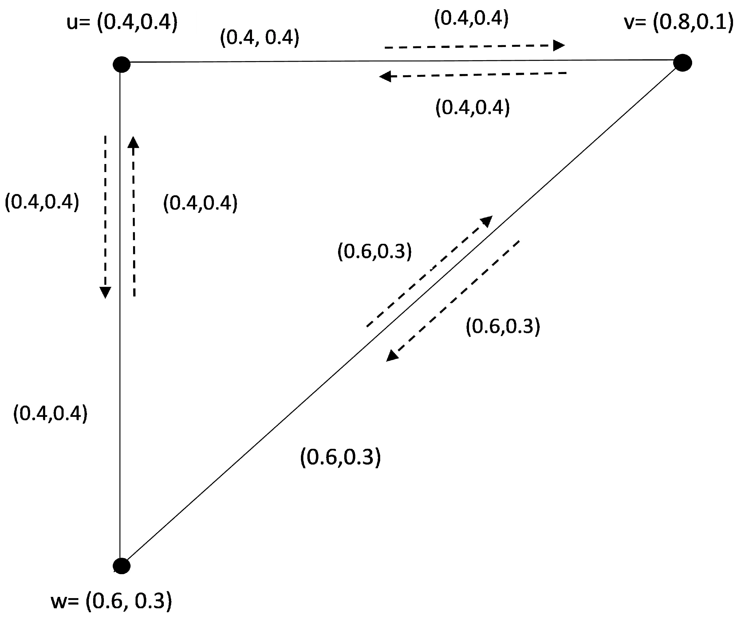
([23]). The greatest influence strength between $u_0$ and $u_1{u}_2$ in an IFIG $\tilde{G}=(V,\lambda ,\mu ,\nu )$ is the highest MVs with the lowest NMVs from all the IFIPs between $u_0$ and $u_1{u}_2$, which is represented by $ICON{N}^{\infty }(u_0,u_1{u}_2)=(ICON{N}^{\zeta \infty }(u_0,u_1{u}_2),ICON{N}^{\eta \infty }(u_0,u_1{u}_2))$ and is defined as $ICON{N}^{\zeta \infty }(u_0,u_1{u}_2)=\vee \left\{ICON{N}^{\zeta n}(u_0,u_1{u}_2)\mid n=1,2,3,\dots \dots ,\infty \right\}$ and $ICON{N}^{\eta \infty }(u_0,u_1{u}_2)=\wedge \left\{ICON{N}^{\eta \infty }(u_0,u_1{u}_2)\mid n=1,2,3,\dots .,\infty \right\}$.

Example 3.

Consider an IFIG given in Figure 3 with $\lambda (u_0=(0.8,0.2)),\lambda (u_1=(0.7,0.3)),\lambda (u_2=(0.6,0.4);\mu (u_0,u_1)=(0.7,0.3),\mu (u_1,u_2)=(0.6,0.4);\mu (u_0,u_0{u}_1)=(0.6,0.2),\nu (u_1,u_1{u}_2)=(0.5,0.2)$ and $\nu (u_0,u_1{u}_2)=(0.4,0.2)$. In this IFIG, there is only one $\overline{IFIP}$ from $u_0$ to $u_1{u}_2$, namely, $u_0,(u_0,u_1{u}_2),u_1{u}_2$ with $\nu (u_0,u_1{u}_2)=(0.4,0.2)$. Clearly, $(u_0,u_1{u}_2)$ is an SIFIP because $(0.4,0.2)=\nu (u_0,u_1{u}_2)>ICON{N}_{G/(u_0,u_1{u}_2)}(u_0,u_1{u}_2)=(0,0)$.

3. Covering and Matching in IFIGs

In this section, we provide detailed discussions on covering and matching in IFIGs by utilizing strong influence paths. In the beginning, we introduce several useful terms related to these notions such as intuitionistic fuzzy effective influence pair (IFIP), $\overline{IFIP}$, SIFINC, WIFIP, SIFIP, $\overline{SIFIP}$, SIS, and SIFIPC. Subsequently, we explore significance characteristics of some special types of IFIGs, such as complete IFIG, bipartite IFIG, and complete bipartite IFIG. Afterward, we discuss the concepts of SM, PSM, etc.

We begin our discussion by introducing the concept of SIFINC of an IFIG based on SIFIP.

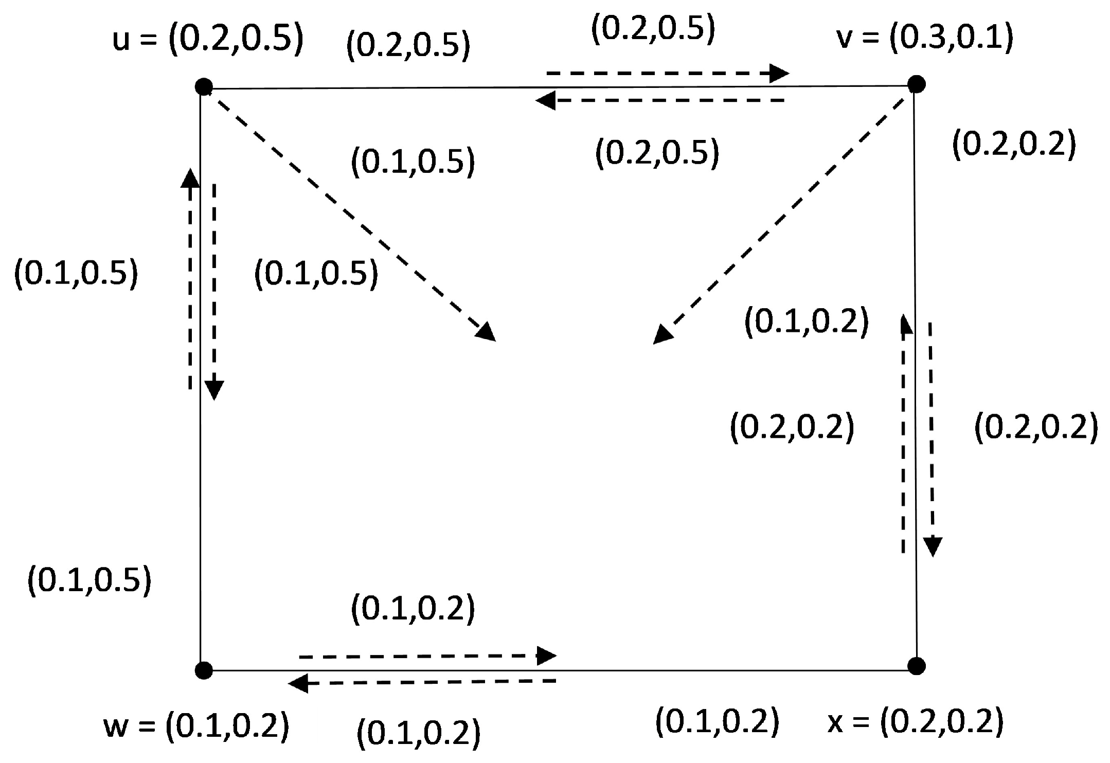
Definition 10.

A collection of nodes D in an IFIG $\tilde{G}=(V,\lambda ,\mu ,\nu )$ that covers all SIFIPs of $\tilde{G}$ is known as SIFINC. The fuzzy weight $\tilde{W}$ of SIFINC D is

$${\tilde{W}}_{nc}=({\tilde{W}}_{nc}^{\zeta }\left(D\right),{\tilde{W}}_{nc}^{\eta }\left(D\right))$$

$${\displaystyle {\tilde{W}}_{nc}=(\sum _{\stackrel{`}{u}\in D}{\zeta }_{\mu }(\stackrel{`}{u},\stackrel{`}{v}\stackrel{`}{w}),\sum _{\stackrel{`}{u}\in D}{\eta }_{\mu }(\stackrel{`}{u},\stackrel{`}{v}\stackrel{`}{w}))}$$

where ${\zeta }_{\mu }(\stackrel{`}{u},\stackrel{`}{v}\stackrel{`}{w})$ is the minimum of the MVs of all SIFIPs and ${\eta }_X(\stackrel{`}{u},\stackrel{`}{v}\stackrel{`}{w})$ is the maximum of the NMVs, respectively, for all SIFIPs of an IFIG $\tilde{G}$ that are incident on $\stackrel{`}{u}$.

Example 4.

Consider an IFIG given in Figure 4 with $\lambda (u_0=(0.7,0.3)),\lambda (u_1=(0.6,0.4)),\lambda (u_2=(0.4,0.5);\mu (u_0,u_1)=(0.6,0.4),\mu (u_1,u_2)=(0.4,0.5);\mu (u_0,u_0{u}_1)=(0.6,0.4),\nu (u_1,u_1{u}_2)=(0.4,0.5)$ and $\nu (u_0,u_1{u}_2)=(0.3,0.5)$. In this IFIG, there is only one $\overline{IFIP}$ from $u_0$ to $u_1{u}_2$, namely, $u_0,(u_0,u_1{u}_2),u_1{u}_2$ with $\nu (u_0,u_1{u}_2)=(0.3,0.5)$. Clearly, $(u_0,u_1{u}_2)$ is an SIFIP because $(0.3,0.5)=\nu (u_0,u_1{u}_2)>ICON{N}_{G/(u_0,u_1{u}_2)}(u_0,u_1{u}_2)=(0,0)$.

By utilizing the concept of SIFINC, we define the notion of SIFINC as follows.

Definition 11.

A set $U\left(\tilde{G}\right)=(U_{\zeta },U_{\eta }$) is a SIFINC number of IFIG if 

$$U_{\zeta }=min\{{\tilde{W}}_{nc}\left(D\right)\mid D \mathit{is\; the\; fuzzy\; weight\; of\; SIFINCs\; of} \tilde{G}\}$$

$$U_{\eta }=max\{{\tilde{W}}_{nc}\left(D\right)\mid D \mathit{is\; the\; fuzzy\; weight\; of\; SIFINCs\; of} \tilde{G}\}$$

In an IFIG $\tilde{G}$, the minimum of MVs and the maximum of NMVs of SNC are known as the minimum SIFINC.

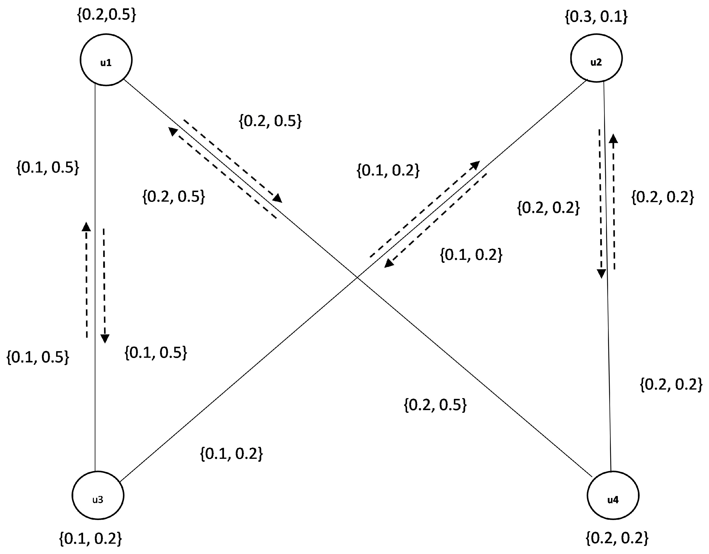
Example 5.

Let us consider an IFIG shown in Figure 5. Here, every IFIP is SIFIP and every SIFINC of IFIG $\tilde{G}$ is $D_1=\{\stackrel{`}{u},\stackrel{`}{u}\stackrel{`}{v}\}$, $D_2=\{\stackrel{`}{v},\stackrel{`}{v}\stackrel{`}{w}\}$, $D_3=\{\stackrel{`}{w},\stackrel{`}{w}\stackrel{`}{u}\}$. Calculations regarding (intuitionistic fuzzy influence) FW of the SIFINC number ${\tilde{W}}_{nc}\left(D\right)$ of an IFIG $\tilde{G}$ are given in

Table 5. Calculating the SIFINC number’s weight.

D	${\tilde{\mathit{W}}}_{\mathit{nc}}^{\mathit{\zeta }}\mathit{\left(}\mathit{D}\mathit{\right)}$	${\tilde{\mathit{W}}}_{\mathit{nc}}^{\mathit{\eta }}\mathit{\left(}\mathit{D}\mathit{\right)}$
$\{\stackrel{`}{u},\stackrel{`}{u}\stackrel{`}{w}\}$	$0.4+0.4$	$0.4+0.4$
$\{\stackrel{`}{v},\stackrel{`}{v}\stackrel{`}{w}\}$	$0.4+0.6$	$0.4+0.3$
$\{\stackrel{`}{w},\stackrel{`}{w}\stackrel{`}{u}\}$	$0.4+0.4$	$0.4+0.4$

and

Table 6. Weight of SIFINC number.

D	${\tilde{\mathit{W}}}_{\mathit{nc}}\mathit{\left(}\mathit{D}\mathit{\right)}$
$\{\stackrel{`}{u},\stackrel{`}{v}\stackrel{`}{w}\}$	$[0.8,0.8]$
$\{\stackrel{`}{w},\stackrel{`}{u}\stackrel{`}{v}\}$	$[1,0.7]$
$\{\stackrel{`}{v},\stackrel{`}{u}\stackrel{`}{w}\}$	$[0.8,0.8]$

. Thus, $U(\tilde{G})=[2.6,2.3].$

Definition 12.

A complete intuitionistic fuzzy incidence graph $\tilde{G}=(V,\lambda ,\mu ,\nu )$ is called a complete IFIG if each node $\stackrel{`}{u}$ has the influence on each edge $\stackrel{`}{v}\stackrel{`}{w}$ with

$${\zeta }_{\nu }(\stackrel{`}{u},\stackrel{`}{v}\stackrel{`}{w})=min\{{\zeta }_W\left(\stackrel{`}{u}\right),{\zeta }_W\left(\stackrel{`}{v}\stackrel{`}{w}\right)\}$$

$${\eta }_{\nu }(\stackrel{`}{u},\stackrel{`}{v}\stackrel{`}{w})=max\{{\eta }_W\left(\stackrel{`}{u}\right),{\eta }_W\left(\stackrel{`}{v}\stackrel{`}{w}\right)\}$$

for all $(\stackrel{`}{u},\stackrel{`}{v}\stackrel{`}{w})\in \nu .$

Definition 13.

If the vertices of any IFIG $\tilde{G}$ can be partitioned into two nonempty subsets ${\widehat{V}}_1$ and ${\widehat{V}}_2$ such that for $\stackrel{`}{u}\in {\widehat{V}}_1$ and $\stackrel{`}{v}\in {\widehat{V}}_2$ with ${\zeta }_{\nu }(\stackrel{`}{u},\stackrel{`}{u}\stackrel{`}{v})=0$, ${\eta }_{\nu }(\stackrel{`}{u},\stackrel{`}{u}\stackrel{`}{v})=0$, then we call it a bipartite-IFIG. Similarly, if for all $\stackrel{`}{u}\in {\widehat{V}}_1$ and $\stackrel{`}{v}\in {\widehat{V}}_2$, we have

$${\zeta }_{\nu }(\stackrel{`}{u},\stackrel{`}{u}\stackrel{`}{v})=min\{{\zeta }_W\left(\stackrel{`}{u}\right),{\zeta }_W\left(\stackrel{`}{u}\stackrel{`}{v}\right)\}$$

$${\eta }_{\nu }(\stackrel{`}{u},\stackrel{`}{u}\stackrel{`}{v})=max\{{\eta }_W\left(\stackrel{`}{u}\right),{\eta }_W\left(\stackrel{`}{u}\stackrel{`}{v}\right)\}$$

then $\tilde{G}$ is said to be a complete-IFIG.

Theorem 1.

If $\tilde{G}=\left(V,\lambda ,\mu ,\nu \right)$ is a complete IFIG, then there exists a $\overline{SIFIP}$ between any two elements of $\lambda \cup \mu$.

Proof. 

We first verify that between any two elements $q,r$ are $\lambda \cup \mu$; there exists an $\overline{IFIP}$. If q,r $\in \lambda$, then s must influence some elements of μ, say yz. Consequently, $\overline{IFIP}$$q,(q,yz),yz,z$ along with the incidence path reaching from z to r; consequently, $\overline{IFIP}$ between q and r. In the same way, if $q\in \lambda$ and $r\in \mu$, then we can obtain a new $\overline{IFIP}$ by joining one influence with the other incidence path. Assume that $q,r\in \mu$. Then we can consider an influence pair at the end nodes of q or r, and thus, there is an $\overline{IFIP}$ between q and r. Hereafter, we have to prove that a complete IFIG has no WIFIP. On the other hand, let $(\tilde{u}=\tilde{v}\tilde{w})$ be an WIFIP. Following Definition i-e, there is an $\overline{IFIP}$ P between $\tilde{u}$ and $\tilde{v}\tilde{w}$ with higher influence strength, say f $\nu (\tilde{u},\tilde{v}\tilde{w})$. Then each of the influence pairs existing in P must has a value ν, which must be greater than or equal to f. Moreover, $\lambda \left(\tilde{u}\right)\ge f$ and $\mu \left(\tilde{v}\tilde{w}\right)\ge f$. Since $\tilde{G}$ is a complete IFIG, we have $\nu (\tilde{u},\tilde{v}\tilde{w})=\wedge \{\lambda \left(\tilde{u}\right),\mu \left(\tilde{v}\tilde{w}\right)\}\ge f$; a contradiction arises. Consequently, every IFIP of $\tilde{G}$ is strong. □

Theorem 2.

If $\tilde{G}=\left(V,\lambda ,\mu ,\nu \right)$ is a complete-IFIG, then

$$U_{\zeta }=(n-1){\zeta }_{\nu }(\stackrel{`}{u},\stackrel{`}{v}\stackrel{`}{w})$$

$$U_{\eta }=(n-1){\eta }_{\nu }(\stackrel{`}{u},\stackrel{`}{v}\stackrel{`}{w})$$

where ${\zeta }_{\nu }(\stackrel{`}{u},\stackrel{`}{v}\stackrel{`}{w})$ represents the MVs, ${\eta }_{\nu }(\stackrel{`}{u},and\stackrel{`}{v}\stackrel{`}{w})$ represents the NMVs of the WIFIP and n is the number of nodes in $\tilde{G}$.

Proof. 

Let $\tilde{G}$ be a complete IFIG. Then, clearly each vertex in $\tilde{G}$ comprises IFIPs that are all SIFIPs. Hence, either of the sets of $(n-1)$ nodes is utilized to form the SIFINC of $\tilde{G}$. Let us assume that a vertex set having minimum MVs and maximum NMVs of $\tilde{G}$ is say $\stackrel{`}{u}$. Assume that the node $\stackrel{`}{u}$ is connected with different nodes ${\stackrel{`}{v}}_1{\stackrel{`}{w}}_1,{\stackrel{`}{v}}_2{\stackrel{`}{w}}_2,\dots ,{\stackrel{`}{v}}_{n-1}{\stackrel{`}{w}}_{n-1}$. Then among all the WIFIPs in $\tilde{G}$, $(\stackrel{`}{u},{\stackrel{`}{v}}_1{\stackrel{`}{w}}_1),(\stackrel{`}{u},{\stackrel{`}{v}}_2{\stackrel{`}{w}}_2),\dots ,(\stackrel{`}{u},{\stackrel{`}{v}}_{n-1}{\stackrel{`}{w}}_{n-1})$ is the $\overline{IFIP}$, which contains MV ${\zeta }_{\nu }(\stackrel{`}{u},\stackrel{`}{v}\stackrel{`}{w})$ and NMV ${\eta }_{\nu }(\stackrel{`}{u},\stackrel{`}{v}\stackrel{`}{w})$, where $\stackrel{`}{v}\in {\stackrel{`}{v}}_1,{\stackrel{`}{v}}_2,\dots ,{\stackrel{`}{v}}_{n-1}$ and $\stackrel{`}{w}\in {\stackrel{`}{w}}_1,{\stackrel{`}{w}}_2,\dots ,{\stackrel{`}{w}}_{n-1}$. Thus, the collection D of vertices represents the set ${\stackrel{`}{v}}_1{\stackrel{`}{w}}_1,{\stackrel{`}{v}}_2{\stackrel{`}{w}}_2,\dots ,{\stackrel{`}{v}}_{n-1}{\stackrel{`}{w}}_{n-1}$ forms SIFINC of $\tilde{G}$ with

$${\displaystyle {\tilde{W}}_{nc}^{\zeta }\left(D\right)=\sum _{\stackrel{`}{v_j}\stackrel{`}{w_j}\in D}{\zeta }_{\nu }(\stackrel{`}{u},\stackrel{`}{v_j}\stackrel{`}{w_j})={\zeta }_{\nu }(\stackrel{`}{u},\stackrel{`}{v_1}{\stackrel{`}{w}}_1)+{\zeta }_{\nu }(\stackrel{`}{u},\stackrel{`}{v_2}{\stackrel{`}{w}}_2)+\dots +{\zeta }_{\nu }(\stackrel{`}{u},{\stackrel{`}{v}}_{n-1}{\stackrel{`}{w}}_{n-1})}$$

where ${\zeta }_{\nu }(\stackrel{`}{u},\stackrel{`}{v_j}{\stackrel{`}{w}}_j),j=1,2,\dots ,(n-1)$ is the minimum of MVs of SIFIPs incident on $\stackrel{`}{v_j}{\stackrel{`}{w}}_j$. Then

$$U_{\zeta }={\zeta }_{\nu }(\stackrel{`}{u},\stackrel{`}{v}\stackrel{`}{w})+{\zeta }_{\nu }(\stackrel{`}{u},\stackrel{`}{v}\stackrel{`}{w})+{\zeta }_{\nu }(\stackrel{`}{u},\stackrel{`}{v}\stackrel{`}{w})$$

where ${\zeta }_{\nu }(\stackrel{`}{u},\stackrel{`}{v}\stackrel{`}{w})$ is the MVs of WIFIP in the IFIG $\tilde{G}$. Hence,

$$U_{\zeta }=(n-1){\zeta }_{\nu }(\stackrel{`}{u},\stackrel{`}{v}\stackrel{`}{w})$$

Similarly,

$${\displaystyle {\tilde{W}}_{nc}^{\eta }\left(D\right)=\sum _{\eta \stackrel{`}{v_j}\stackrel{`}{w_j}\in D}{\eta }_{\nu }(\stackrel{`}{u},{\stackrel{`}{v}}_j{\stackrel{`}{w}}_j)={\eta }_{\nu }(\stackrel{`}{u},\stackrel{`}{v_1}{\stackrel{`}{w}}_1)+{\eta }_{\nu }(\stackrel{`}{u},\stackrel{`}{v_2}{\stackrel{`}{w}}_2)+\dots +{\eta }_{\nu }(\stackrel{`}{u},{\stackrel{`}{v}}_{n-1}{\stackrel{`}{w}}_{n-1})}$$

where ${\eta }_{\nu }(\stackrel{`}{u},\stackrel{`}{v_j}{\stackrel{`}{w}}_j),j=1,2,\dots ,(n-1)$ represents the maximum NMVs of the SIFIPs incident on $\stackrel{`}{v_j}{\stackrel{`}{w}}_j$, similarly. Thus,

$$U_{\eta }={\eta }_{\nu }(\stackrel{`}{u},\stackrel{`}{v}\stackrel{`}{w})+{\eta }_{\nu }(\stackrel{`}{u},\stackrel{`}{v}\stackrel{`}{w})+{\eta }_{\nu }(\stackrel{`}{u},\stackrel{`}{v}\stackrel{`}{w})$$

where ${\eta }_{\nu }(\stackrel{`}{u},\stackrel{`}{v}\stackrel{`}{w})$ represent the NMVs of WIFIP in the IFIG $\tilde{G}$. Thus,

$$U_{\eta }=(n-1){\eta }_{\nu }(\stackrel{`}{u},\stackrel{`}{v}\stackrel{`}{w})$$

□

Theorem 3.

In a complete bipartite IFIG, $\tilde{G}$ can be divided into two nonempty subsets ${\widehat{V}}_1$ and ${\widehat{V}}_2$. Then

$$U_{\zeta }\left(\tilde{G}\right)=min\{{\tilde{W}}_{nc}^{\zeta }\left({\widehat{V}}_1\right),{\tilde{W}}_{nc}^{\zeta }\left({\widehat{V}}_2\right)\}$$

$$U_{\eta }\left(\tilde{G}\right)=max\{{\tilde{W}}_{nc}^{\eta }\left({\widehat{V}}_1\right),{\tilde{W}}_{nc}^{\eta }\left({\widehat{V}}_2\right)\}$$

Proof. 

  Assume that $\tilde{G}$ is a complete bipartite IFIG. Then each of its IFIP is a SIFIP. Let us consider two non-empty subsets of a vertex set ${\widehat{V}}_1$ and ${\widehat{V}}_2$, where each node in ${\widehat{V}}_1$ is connected to every other node in ${\widehat{V}}_2$ and conversely. The union of all IFIPs that has influence on each of its vertex in ${\widehat{V}}_1$ and the collection of all paths that have influence on each vertex in ${\widehat{V}}_2$ form the collection of IFIPs in a complete bipartite graph $\tilde{G}$. Furthermore, ${\widehat{V}}_1$, ${\widehat{V}}_2$, and their union ${\widehat{V}}_1\cup {\widehat{V}}_2$ are IFIG in $\tilde{G}$. Clearly,

$${\tilde{W}}_{nc}^{\zeta }({\widehat{V}}_1\cup {\widehat{V}}_2)>{\tilde{W}}_{nc}^{\zeta }\left({\widehat{V}}_1\right)$$

$${\tilde{W}}_{nc}^{\zeta }({\widehat{V}}_1\cup {\widehat{V}}_2)>{\tilde{W}}_{nc}^{\zeta }\left({\widehat{V}}_2\right)$$

Hence,

$$U_{\zeta }\left(\tilde{G}\right)=min\{{\tilde{W}}_{nc}^{\zeta }\left({\widehat{V}}_1\right),{\tilde{W}}_{nc}^{\zeta }\left({\widehat{V}}_2\right)\}.$$

Additionally, we have

$${\tilde{W}}_{nc}^{\eta }({\widehat{V}}_1\cup {\widehat{V}}_2)<{\tilde{W}}_{nc}^{\eta }\left({\widehat{V}}_1\right)$$

$${\tilde{W}}_{nc}^{\eta }({\widehat{V}}_1\cup {\widehat{V}}_2)<{\tilde{W}}_{nc}^{\eta }\left({\widehat{V}}_2\right)$$

Hence,

$$U_{\eta }\left(\tilde{G}\right)=max\{{\tilde{W}}_{nc}^{\eta }\left({\widehat{V}}_1\right),{\tilde{W}}_{nc}^{\eta }\left({\widehat{V}}_2\right)\}$$

□

Definition 14.

Let $\tilde{G}=(V,\lambda ,\mu ,\nu )$ be an IFIG. Two nodes are considered as SI in $\tilde{G}$ if there are no SIFIPs between them. A set of nodes that contains any two vertices that are SI is called SIS.

Based on SIS, we describe its FW as follows:

Definition 15.

The FW of SIS D in an IFIG $\tilde{G}$ can be described as

$${\tilde{W}}_{is}=({\tilde{W}}_{is}^{\zeta }\left(D\right),{\tilde{W}}_{is}^{\eta }\left(D\right))$$

or

$${\displaystyle {\tilde{W}}_{is}=(\sum _{\stackrel{`}{u}\in D}{\zeta }_{\mu }(\stackrel{`}{u},\stackrel{`}{v}\stackrel{`}{w}),\sum _{\stackrel{`}{u}\in D}{\eta }_{\mu }(\stackrel{`}{u},\stackrel{`}{v}\stackrel{`}{w}))}$$

where $\zeta \mu (\stackrel{`}{u},\stackrel{`}{v}\stackrel{`}{w})$ represents the minimum of the MVs of all SIFIPs, while ${\eta }_{\mu }(\stackrel{`}{u},\stackrel{`}{v}\stackrel{`}{w})$ is a maximum of the NMVs of all SIFIPs in the IFIG $\tilde{G}$ that are incident on $\stackrel{`}{u}$. Then the SI number $\nu \widetilde{\left(G\right)}={\nu }_{\zeta },{\nu }_{\eta }$ satisfies

$${\nu }_{\zeta }=max\{{\tilde{W}}_{is}^{\zeta }\left(D\right)\mid D \mathit{is\; the\; SISs\; of\; nodes\; in} \tilde{G}\}$$

$${\nu }_{\eta }=min\{{\tilde{W}}_{is}^{\eta }\left(D\right)\mid D \mathit{is\; the\; SISs\; of\; nodes\; in} \tilde{G}\}$$

The maximum SIS in an IFIG $\tilde{G}$ is SIS containing a maximum MVs and minimum NMVs.

Theorem 4.

If $\tilde{G}=(V,\lambda ,\mu ,\nu )$ is a complete IFIG, then

$$\nu \left(\tilde{G}\right)=({\zeta }_{\mu }(\stackrel{`}{u},\stackrel{`}{v}\stackrel{`}{w}),{\eta }_{\mu }(\stackrel{`}{u},\stackrel{`}{v}\stackrel{`}{w}))$$

where ${\zeta }_{\mu }(\stackrel{`}{u},\stackrel{`}{v}\stackrel{`}{w})$ denotes MVs and ${\eta }_{\mu }(\stackrel{`}{u},\stackrel{`}{v}\stackrel{`}{w})$ represents NMVs of the weakest path in $\tilde{G}$.

Proof. 

By assumption, each of its path is SIFIPs and every vertex in $\tilde{G}$ is linked to the rest of the vertices. Thus, $D=\left\{\stackrel{`}{v}\stackrel{`}{w}\right\}$ is a unique SIS for all $\stackrel{`}{v}\stackrel{`}{w}\in V\times V$. □

Theorem 5.

Let $\tilde{G}$ be a set of vertices in a complete bipartite IFIG $\tilde{G}=(V,\lambda ,\mu ,\nu )$ that can be partitioned into the two non-empty subsets ${\widehat{V}}_1$ and ${\widehat{V}}_2$. Then

$${\nu }_{\zeta }\left(\tilde{G}\right)=min\{{\tilde{W}}_{is}^{\zeta }\left({\widehat{V}}_1\right),{\tilde{W}}_{is}^{\zeta }\left({\widehat{V}}_2\right)\}$$

$${\nu }_{\eta }\left(\tilde{G}\right)=max{{\tilde{W}}_{is}^{\eta }\left({\widehat{V}}_1\right),{\tilde{W}}^{\eta }}_{is}\left({\widehat{V}}_2\right)$$

Proof. 

Let $\tilde{G}$ be a complete bipartite IFIG. It implies that every path in $\tilde{G}$ is a SIFIP. Furthermore, each vertex in ${\widehat{V}}_1$ is connected to every other vertex in ${\widehat{V}}_2$, and each vertex in ${\widehat{V}}_2$ is linked to every other vertex in ${\widehat{V}}_1$. Both ${\widehat{V}}_1$ and ${\widehat{V}}_2$ are SISs in $\tilde{G}$, which completes the proof. □

Theorem 6.

Let $\tilde{G}$ be an IFIG without an isolated node. Then

$$U_{\zeta }+{\nu }_{\zeta }={\tilde{W}}^{\zeta }\left(V\right)$$

$$U_{\eta }+{\nu }_{\eta }={\tilde{W}}^{\eta }\left(V\right)$$

Proof. 

Let us assume that $M_0$ is the minimum SIFINC of $\tilde{G}$. Then

$$U_{\zeta }={\tilde{W}}^{\zeta }\left(M_0\right)$$

$$U_{\eta }={\tilde{W}}^{\eta }\left(M_0\right)$$

and $V-M_0$ forms the SIS of nodes. Furthermore, $V-M_0$ consists of the nodes that are incident on SIFIPs of $\tilde{G}$. Thus,

$$\begin{array}{c}\hfill {\nu }_{\zeta }\ge {\tilde{W}}^{\zeta }(V-M_0)={\tilde{W}}^{\zeta }\left(V\right)-U_{\zeta }\Rightarrow U_{\zeta }+{\nu }_{\zeta }\ge {\tilde{W}}^{\zeta }\left(V\right)\\ \hfill {\nu }_{\eta }\le {\tilde{W}}^{\eta }(V-M_0)={\tilde{W}}^{\eta }\left(V\right)-U_{\eta }\Rightarrow U_{\eta }+{\nu }_{\eta }\le {\tilde{W}}^{\eta }\left(V\right)\end{array}$$

(1)

Consider $M_0$ as the maximum SIS of $\tilde{G}$; i.e., $M_0$ consists of the nodes that are not neighbor to each other by SIFIPs. Therefore, $V-M_0$ consists of the vertices that cover every SIFIP of $\tilde{G}$. Thus, $V-M_0$ represents SNC of $\tilde{G}$. Furthermore, $U_{\zeta }$ is the minimum MVs, and $U_{\eta }$ is the maximum NMVs.

$$\begin{array}{c}\hfill U_{\zeta }\le {\tilde{W}}^{\zeta }(V-M_0)={\tilde{W}}^{\zeta }\left(V\right)-{\nu }_{\zeta }\Rightarrow U_{\zeta }+{\nu }_{\zeta }\le {\tilde{W}}^{\zeta }\left(V\right)\\ \hfill U_{\eta }\ge {\tilde{W}}^{\eta }(V-M_0)={\tilde{W}}^{\eta }\left(V\right)-{\nu }_{\eta }\Rightarrow U_{\eta }+{\nu }_{\eta }\ge {\tilde{W}}^{\eta }\left(V\right)\end{array}$$

(2)

From (1) and (2), we have

$$U_{\zeta }+{\nu }_{\zeta }={\tilde{W}}^{\zeta }\left(V\right)$$

$$U_{\eta }+{\nu }_{\eta }={\tilde{W}}^{\eta }\left(V\right)$$

, which completes the proof. □

Example 6.

Consider a strong IFIG given in Figure 6. Clearly, all SISs are $D_1=\{\stackrel{`}{u},\stackrel{`}{u}\stackrel{`}{x}\}$, $D_2=\{\stackrel{`}{v},\stackrel{`}{v}\stackrel{`}{w}\}$; also, FWs of SI numbers of IFIG $\tilde{G}$ are given in

Table 7. Weight of SI number.

D	${\tilde{\mathit{W}}}_{\mathit{is}}^{\mathit{\nu }}\mathit{\left(}\mathit{D}\mathit{\right)}$	${\tilde{\mathit{W}}}_{\mathit{is}}^{\mathit{\eta }}\mathit{\left(}\mathit{D}\mathit{\right)}$	${\tilde{\mathit{W}}}_{\mathit{is}}\mathit{\left(}\mathit{D}\mathit{\right)}$
$\{\stackrel{`}{u},\stackrel{`}{u}\stackrel{`}{x}\}$	$0.1+0.2$	$0.5+0.5$	$[0.3,1]$
$\{\stackrel{`}{v},\stackrel{`}{v}\stackrel{`}{w}\}$	$0.2+0.1$	$0.5+0.2$	$[0.3,0.7]$

. We conclude $\nu \left(\tilde{G}\right)=[0.6,1.7]$.

Definition 16.

An SIFIPC of an IFIG $\tilde{G}$ with no isolated node is the set $\tilde{B}$ of SIFIPs, which covers every node in IFIG $\tilde{G}$. The SIFIPC $\tilde{B}$ FW $\tilde{W}$ can be described as

$${\tilde{W}}_{pc}=({\tilde{W}}_{pc}^{\zeta }\left(\tilde{B}\right),{\tilde{W}}_{pc}^{\eta }\left(\tilde{B}\right))$$

$${\displaystyle {\tilde{W}}_{pc}=(\sum _{(\stackrel{`}{u},\stackrel{`}{v}\stackrel{`}{w})\in \tilde{B}}{\zeta }_X(\stackrel{`}{u},\stackrel{`}{v}\stackrel{`}{w}),\sum _{(\stackrel{`}{u},\stackrel{`}{v}\stackrel{`}{w})\in \tilde{B}}{\eta }_X(\stackrel{`}{u},\stackrel{`}{v}\stackrel{`}{w}))}$$

where ${\zeta }_X(\stackrel{`}{u},\stackrel{`}{v}\stackrel{`}{w})$ is the minimum of the MVs of SIFIPs and ${\eta }_X(\stackrel{`}{u},\stackrel{`}{v}\stackrel{`}{w})$ is the maximum of the NMVs of SIFIPs.

A set $U\left(G\right)=(U_{\zeta },U_{\eta })$ is an SIFIPC number of IFIG if 

$$U_{\zeta }=min\{{\tilde{W}}_{pc}^{\zeta }\left(\tilde{B}\right)\mid \tilde{B} \mathit{is\; SIFIPC\; of} \tilde{G}\}$$

$$U_{\eta }=max\{{\tilde{W}}_{pc}^{\eta }\left(\tilde{B}\right)\mid \tilde{B} \mathit{is\; SIFIPC\; of} \tilde{G}\}$$

In IFIG $\tilde{G}$, a minimum SIFIPC contains a minimum MV and a maximum NMV.

Theorem 7.

Let $\tilde{G}$ be a complete IFIG. Then

$$U_{\zeta }=min\{{\tilde{W}}_{pc}^{\zeta }\left(\tilde{B}\right)\mid \tilde{B} \mathit{is\; SIFIPCs\; of} \tilde{G} \mathit{with} \mid \tilde{B}\mid \ge \lceil {\displaystyle \frac{\widehat{n}}{2}}\rceil \}$$

$$U_{\eta }=max\{{\tilde{W}}_{pc}^{\eta }\left(\tilde{B}\right)\mid \tilde{B} \mathit{is\; SIFIPCs\; of} \tilde{G} \mathit{with} \mid \tilde{B}\mid \ge \lceil {\displaystyle \frac{\widehat{n}}{2}}\rceil \}$$

where $\widehat{n}$ represents the number of vertices in $\tilde{G}$.

Proof. 

Assuming that $\tilde{G}$ is complete-IFIG, then each of its vertex is linked to the rest of vertices, and all of its IFIPs are SIFIPs. There are the same number of paths in SIFIPC in both the graphs, as each IFIP in both the IFIG $\tilde{G}$ and a crisp graph $G^{★}$ is an SIFIP. Then $\lceil {\displaystyle \frac{\widehat{n}}{2}}\rceil$ is the SIFIPC number of the crisp graph $G^{★}$. Thus, in SIFIPC of $\tilde{G}$, $\lceil {\displaystyle \frac{\widehat{n}}{2}}\rceil$ is a minimum path. □

Theorem 8.

Let $\tilde{\kappa }$ be the set of vertices of a complete bipartite IFIG $\tilde{G}=(V,\lambda ,\mu ,\nu )$ that can be partitioned into ${\widehat{V}}_1$ and ${\widehat{V}}_2$. Then

$$U_{\zeta }\left(\tilde{\kappa }\right)=min\{{\tilde{W}}_{pc}^{\zeta }\left(\tilde{B}\right)\mid \tilde{B} \mathit{is\; SIFIPC\; in} \tilde{\kappa } \mathit{with} \mid \tilde{B}\mid \ge max\{\mid {\widehat{V}}_1\mid ,\mid {\widehat{V}}_2\mid \}\}$$

$$U_{\eta }\left(\tilde{\kappa }\right)=max\{{\tilde{W}}_{pc}^{\eta }\left(\tilde{B}\right)\mid \tilde{B} \mathit{is\; SIFIPC\; in} \tilde{\kappa } \mathit{with} \mid \tilde{B}\mid \ge max\{\mid {\widehat{V}}_1\mid ,{\widehat{V}}_2\mid \}\}$$

Proof. 

Let us consider a complete bipartite IFIG $\tilde{G}$. Then each of its node in ${\widehat{V}}_1$ is connected to every other node in ${\widehat{V}}_2$, and every IFIP is SIFIP. Since every IFIP in IFIG $\tilde{G}$ is SIFIP and a crisp graph $G^{★}$, both have the same numbers of strong path covers (SIFIPCs). Then the SIFIPC number of ${\tilde{\kappa }}^{★}$ is $max\{\mid {\widehat{V}}_1\mid ,\mid {\widehat{V}}_2\mid \}$. Hence, the minimum number of paths is equal to the $max\{\mid {\widehat{V}}_1\mid ,\mid {\widehat{V}}_2\mid \}$ in the SIFIPC of $\tilde{\kappa }$. □

Definition 17.

SIFIPCs T in an IFIG $\tilde{G}=(V,\lambda ,\mu ,\nu )$ are known as a SIS if there are no two paths that share a node. We call such a set T a strong matching in $\tilde{G}$.

The FW of SM is as follows.

Definition 18.

A set T is an SM in IFIG, and if $(\stackrel{`}{u},\stackrel{`}{v}\stackrel{`}{w})\in T$, then T is a $\stackrel{`}{u}$ SM to $\stackrel{`}{v}\stackrel{`}{w}$. The (intuitionistic fuzzy influence) FW $\tilde{W}$ of SM T is as follows:

$${\tilde{W}}_{sm}\left(T\right)=({\tilde{W}}_{sm}^{\zeta }\left(T\right),{\tilde{W}}_{sm}^{\eta }\left(T\right))$$

$${\displaystyle {\tilde{W}}_{sm}\left(T\right)=(\sum _{(\stackrel{`}{u},\stackrel{`}{v}\stackrel{`}{w})\in T}{\zeta }_Y(\stackrel{`}{u},\stackrel{`}{v}\stackrel{`}{w}),\sum _{(\stackrel{`}{u},\stackrel{`}{v}\stackrel{`}{w})\in T}{\eta }_Y(\stackrel{`}{u},\stackrel{`}{v}\stackrel{`}{w}))}$$

A collection $\nu \left(\tilde{G}\right)=({\nu }_{\zeta },{\nu }_{\eta })$ is an SM in IFIG if

$${\nu }_{\zeta }=max\{{\tilde{W}}_{is}^{\zeta }\left(T\right)\mid T \mathit{is\; the\; SM\; of} \tilde{G}\}$$

$${\nu }_{\eta }=min\{{\tilde{W}}_{is}^{\eta }\left(T\right)\mid T \mathit{is\; the\; SM\; of} \tilde{G}\}$$

The maximum SM in IFIG $\tilde{G}$ is SM with the maximum MV and minimum NMV.

Theorem 9.

If $\tilde{G}=(V,\lambda ,\mu ,\nu )$ is a complete IFIG, then

$${\nu }_{\zeta }=max\{{\tilde{W}}_{sm}^{\zeta }\left(T\right)\mid T \mathit{is\; SM\; with} \mid T\mid \le \lceil {\displaystyle \frac{\widehat{n}}{2}}\rceil \}$$

$${\nu }_{\eta }=min\{{\tilde{W}}_{sm}^{\eta }\left(T\right)\mid T \mathit{is\; SM\; with} \mid T\mid \le \lceil {\displaystyle \frac{\widehat{n}}{2}}\rceil \}$$

where $\widehat{n}$ represents the number of nodes in $\tilde{G}$.

Proof. 

Assuming that $\tilde{G}$ is a complete IFIG, it implies that each of its vertex must be connected to every other vertex, and all of its paths are $\overline{SIFIPs}$. Since every path in an IFIG $\tilde{G}$ and an underlying graph $G^{★}$ are an SP, the number of paths in the SM is the same in both graphs. Then the SM number of the underlying graph $G^{★}$ is $\lceil {\displaystyle \frac{\widehat{n}}{2}}\rceil$. Hence, the maximum number of paths in the strong matching of $\tilde{G}$ is $\lceil {\displaystyle \frac{\widehat{n}}{2}}\rceil$. □

Before describing Theorem 10, it is important to highlight that the condition requiring $\tilde{G}$ to be partitioned into two non-empty subsets ${\widehat{V}}_1$ and ${\widehat{V}}_2$ is essential, as it defines the bipartite structure of the graph. Moreover, without such a partition, $\tilde{G}$ cannot be classified as a complete bipartite IFIG. Furthermore, the maximum size of a strong matching (SM) in $\tilde{G}$ is constrained by $min\{\mid {\widehat{V}}_1\mid ,\mid {\widehat{V}}_2\mid \}$, a condition that only holds if the vertex set is properly divided into these two subsets.

Theorem 10.

Let $\tilde{G}$ be a complete bipartite IFIG that can be partitioned into two nonempty subsets ${\widehat{V}}_1$ and ${\widehat{V}}_2$. Then

$${\nu }_{\zeta }\left(\tilde{G}\right)=max\{{\tilde{W}}_{sm}^{\zeta }\left(T\right)\mid T \mathit{is\; SM\; in} \tilde{G} \mathit{with} \mid T\mid \le min\{\mid {\widehat{V}}_1\mid ,\mid {\widehat{V}}_2\mid \}\}$$

$${\nu }_{\eta }\left(\tilde{G}\right)=min\{{\tilde{W}}_{sm}^{\eta }\left(T\right)\mid T \mathit{is\; SM\; in} \tilde{G} \mathit{with} \mid T\mid \le min\{\mid {\widehat{V}}_1\mid ,\mid {\widehat{V}}_2\mid \}\}$$

Proof. 

Assume that $\tilde{G}$ is a complete bipartite-IFIG. It implies that each of its IFIPs is SIFIPs and every vertex of ${\widehat{V}}_1$ is linked to each vertex of ${\widehat{V}}_2$. That is because every $\overline{IFIP}$ in IFIG $\tilde{G}$ and an underlying graph $G^{★}$ are strong $\overline{IFIP}$. Thus, in SM, there is the same number of paths for both graphs. The SM number of ${\tilde{G}}^{★}$ is $max\{\mid {\widehat{V}}_1\mid ,\mid {\widehat{V}}_2\mid \}$. Therefore, $\tilde{G}$ is the maximum number of paths in SM, which is $min\{\mid {\widehat{V}}_1\mid ,\mid {\widehat{V}}_2\mid \}$. □

Extending the term SM, now we introduce the concept of PSM.

Definition 19.

Let $\tilde{G}=(V,\lambda ,\mu ,\nu )$ be an IFIG and M be a SM in $\tilde{G}$. Then, M is called PSM if every vertex of M in $\tilde{G}$ is strongly matched to some vertices in $\tilde{G}$.

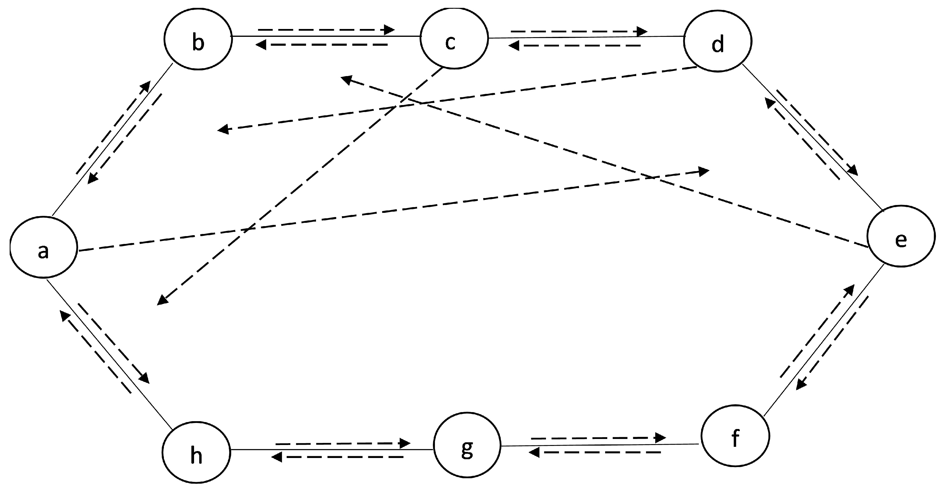
Example 7.

Refer to an IFIG given in Figure 7. Each path is SIFIP, and $M_1$ and $M_2$ are PSM. All SMs of $\tilde{G}$ are $M_1=\left\{\{u_1,u_1{u}_3\}\{u_2,u_2{u}_4\}\right\}$, $M_2=\left\{\{u_1,u_1{u}_4\}\{u_2,u_2{u}_3\}\right\}$, $M_3=\left\{\{u_1,u_1{u}_3\}\{u_1,u_1{u}_4\}\{u_2,u_2{u}_4\}\right\}$, $M_4=\left\{\{u_1,u_1{u}_3\}\{u_3,u_3{u}_2\}\{u_2,u_2{u}_4\}\right\}$. The (intuitionistic fuzzy influence) FW of SM is calculated in

Table 8. Calculating the weight of SM.

M	${\stackrel{\mathit{`}}{\mathit{W}}}_{\mathit{sm}}^{\mathit{\zeta }}\mathit{\left(}\mathit{M}\mathit{\right)}$	${\stackrel{\mathit{`}}{\mathit{W}}}_{\mathit{sm}}^{\mathit{\eta }}\mathit{\left(}\mathit{M}\mathit{\right)}$	${\stackrel{\mathit{`}}{\mathit{W}}}_{\mathit{sm}}\mathit{\left(}\mathit{M}\mathit{\right)}$
$M_1$	$0.1+0.1+0.2+0.2$	$0.5+0.5+0.5+0.2$	$\langle [0.6,1.7]\rangle$
$M_2$	$0.1+0.2+0.2+0.1$	$0.5+0.5+0.5+0.2$	$\langle [0.6,1.7]\rangle$
$M_3$	$0.1+0.1+0.1+0.2+0.2+0.2$	$0.5+0.5+0.5+0.5+0.5+0.2$	$\langle [0.9,2.7]\rangle$
$M_4$	$0.1+0.1+0.1+0.1+0.2+0.2$	$0.5+0.5+0.5+0.2+0.5+0.2$	$\langle [0.8,2.4]\rangle$

. Hence, $\nu \left(M\right)=\langle [0.2,1.3]\rangle$, $U\left(M\right)=\langle [0.4,1.2]\rangle$

4. Application

In the education field, social networks can be defined as groups of students or educators that are connected by common academic interests and goals. Each participant in the network, whether a student or an educator, is considered an actor. The interactions and relationships between these actors define the social network usually focusing on the subjects of the study, research interests, or collaborative projects. Representing these social networks as graphs helps us analyze how many students are studying specific subjects (represented by vertices) and how these subjects influence each other (represented by edges) to facilitate exhibitions, seminars, etc., encouraging greater student participation in such activities. Assume that a community represents a group of students and educators who are heavily involved and interconnected in a specific subjects area such as node a, node f, and node b. Overlapping in these communities is common, reflecting students and educators who participate in multiple subjects. For Example, a student might be part of communities in both node a and node f due to shared academic interests or joint research projects. Moreover, the strength of influence within these communities can be evaluated using metrics like covering and matching in graphs. For example, the impact of a node b community could be measured by the average participation of its members in subject-related activities such as seminars and academic conferences. On the other hand, in academic environments, exhibitions serve as platforms for students and educators to present their work, fostering deeper engagement with their academic communities. When educational institutions organize such exhibitions at a common meeting spot, the challenge is to arrange as many different exhibitions as possible simultaneously while ensuring that each institution hosts only one exhibition at any given time. Moreover, the exhibitions must be scheduled such that overlapping exhibitions do not conflict with students’ or educators’ participation, considering that they may belong to multiple academic communities. Hence, for every event, each group influences the other, and their impact is not certain. Consequently, analyzing the strength of one group’s influence on the other using a classical graph does not yield precise results. We address the overlapping interests involving uncertainties in the participation of these academic communities through IFIGs in this study. Unlike FGs that use only membership values, IFIGs consider both membership and non-membership values, providing a more comprehensive analysis of the strength of influence and engagement in community activities.

To measure the total impact of a community on its members, we consider two key factors: the average of the number of members present in meetings and those members who did not attend the meeting are depicted in

Table 9. Data set.

Vertices (Communities)	No. of Members	Average No. of  Members Present  in Meeting	No. of Members Not Present in Meeting
a	40	37	3
b	60	53	7
c	55	50	5
d	80	65	15
e	45	37	8
f	35	29	6
g	50	45	5
h	42	36	6

. These variables are crucial because members’ participation in meetings significantly influences the effectiveness of the community in promoting academic activities. For instance, the ratio of members present at meetings to the total number of community members indicates the effectiveness of the community’s promotions, while the ratio of members absent provides insight into ineffectiveness. To illustrate this, let us consider the node a community shown in

Table 10. The IFIG of academic communities.

$\mathit{Vertices}\left(\mathit{Communities}\right)$	$\mathit{IFIG}\mathit{Corresponding}\mathit{to}\mathit{Each}\mathit{Community}$
a	$[0.9,0.1]$
b	$[0.7,0.3]$
c	$[0.8,0.2]$
d	$[0.3,0.6]$
e	$[0.7,0.3]$
f	$[0.8,0.2]$
g	$[0.8,0.1]$
h	$[0.6,0.4]$

. The effectiveness of the community can be represented by the ratio of students attending meetings to the total membership. If 80% of the members regularly attend the meetings, this suggests that the community is highly effective in promoting engagement and knowledge sharing. On the other hand, the 20% of members who are not attending the meetings represent the ineffective portion, indicating lower engagement and participation, which could reduce the overall academic progress of the community. The relationships between communities are also influenced by their degree of collaboration and shared interests. These inter-community influences are dealt through IFIGs. For example, the interaction between the node a and node f communities might have an effectiveness of 75% to 85% (indicating strong collaborative efforts), while a neutral relationship (with membership values ranging from 10% to 20%) percent reflects a moderate impact. Alternatively, a relationship with 5% to 10% ineffectiveness may suggest that a small portion of members are disengaged or not participating in joint activities. These values are shown in

Table 11. The IFIG relation between academic communities.

$\mathit{Edges}$	$\mathit{IFIG}$	$\mathit{Edges}$	$\mathit{IFIG}$
$ab$	$[0.7,0.3]$	$bc$	$[0.7,0.3]$
$fg$	$[0.8,0.2]$	$cd$	$[0.2,0.6]$
$ef$	$[0.7,0.3]$	$de$	$[0.3,0.7]$
$gh$	$[0.6,0.4]$	$ha$	$[0.7,0.2]$

. By evaluating these membership and non-membership values across the different communities and their interactions, we can better understand the overall impact of the community’s efforts, including how effectively they promote academic success, and where interventions may be necessary to improve participation and engagement.

Through the maximum SIS, we suggest the numbers of exhibitions that can be held at the same time across different subject communities to ensure maximum participation. Identifying the maximal independent set (SIS) within these networks could help in highlighting the largest groups of subjects or academic interests where no two are closely related in terms of participation or interaction. Normally, no polynomial algorithm exists for finding the maximal IS in any arbitrary graph. This shows that obtaining the maximal IS collection in a short period of time is not possible. Thus, we find the maximum SIS of IFIG by calculating fuzzy weights. It includes all fundamentals and maximal SISs because each path is $\overline{SIFIP}$. We also provide an algorithm (Algorithm 1) to determine the maximal SIS.

Algorithm 1 Finding the maximum SIS S of an IFIG with any arbitrary vertex d

Step 1. Consider d be a vertex included in S. Delete all the vertices adjoining to d. Step 2. Now study different arbitrary vertex in the left over graph included in S. Now different IS, containing d, can be attained depending on the vertex choose from the remaining graph contained in S. Step 3. For selection of all possible vertices repeat step 2. Step 4. Revisit the previous choices and find alternative vertices from the reduced graphs to check all of possible combinations. Save the size of each of the SIS. Step 5. From all selected ISs, select that one which has a largest number of vertices in order to represent the maximum SIS S. Step 6. To improve the efficiency in larger graphs, choose the next vertex using a scoring strategy that prioritizes low total MVs and high NMVs with its neighbors. Give preference to vertices having higher scores, the score can be calculated as: $$Score\left(v\right)=\sum _{u\in N\left(v\right)}(1-\zeta (u,v)+\eta (u,v))$$ Step 7. Continue the recursive, heuristic-guided selection process until no vertices can be added without breaching the independence condition. Return the largest SIS identified.

Complexity analysis of an algorithm.

The algorithm provided for identifying the maximum SIS in an IFIG is computationally intensive because of its combinatorial complexity. At each stage, the problem size is reduced by selecting a vertex and removing its adjacent vertices. However, since this must be performed for every possible vertex selection, the number of resulting combinations grows exponentially. Because the graph is arbitrary and the choice of vertices greatly influences the result, a thorough exploration of all possibilities is often necessary to guarantee maximality. In general, its time complexity can reach up to $O\left(2^n\right)$, where n represents the number of vertices. The maximum SISs are $D_1=\{a,ed\}$, $D_2=\{c,ah\}$, $D_3=\{e,bc\}$, and $D_4=\{d,ab\}$. Fuzzy weights of the sets presented above are $\stackrel{`}{W}\left(D_1\right)=[1.1,0.9]$, $\stackrel{`}{W}\left(D_2\right)=[0.7,1.0]$, $W\left(D_3\right)=[1.0,1.0]$, and $\stackrel{`}{W}\left(D_4\right)=[1.0,1.0]$.

Thus, $D_1$ has the maximum MV and minimum NMV, and hence, it can be picked as the most suitable choice. Therefore, $D_1$ includes the number of students or educators that are at the maximum in different subject communities; i.e., node a, node e, and node d are involved in SI different subject communities.

Intuitionistic fuzzy influence graphs (IFIGs) are useful for modeling communities based on shared subjects, like academic fields. By representing students as nodes and their interactions or common interests as connections, IFIGs can show the different levels of influence and involvement within these communities. This method allows for a detailed analysis of how students engage with various subjects, helping to plan specific actions to improve learning results. In educational settings, exhibitions serve as platforms where students present their projects, experiments, and models to peers, teachers, and parents. These exhibitions provide opportunities for students to demonstrate their understanding of scientific concepts through practical applications and creative displays. Integrating exhibitions into the analysis of subject-based communities can offer valuable insights into student engagement and learning outcomes. By observing how students participate in and contribute to exhibitions related to specific subjects, educators can identify areas where students are highly engaged and areas that may require additional support or resources. This approach enables a more comprehensive understanding of student involvement and can inform strategies to enhance educational experiences. In the above-mentioned scenario, assume that educational institutions planned an exhibition in a common meeting spot to familiarize students or educators with their academic programs. Students from these institutions may belong to many academic communities. The purpose is to organize as many different exhibitions as possible simultaneously, ensuring that, during any specific time period, each institution hosts only one exhibition, while other exhibitions are held at various intervals of time. All of these factors involve uncertainty, and hence, IFIGs are an effective tool for analyzing the strength of influence. However, since FIGs use a single membership value, they do not account for the extent to which the influenced group is not influenced by a specific group. However, IFIGs consider both membership and non-membership values, allowing for a more comprehensive and precise analysis. Thus, IFIGs would provide better and more accurate results compared with FIGs.

Verification of Our Presented Model via the TOPSIS Method

To identify influential academic actors and their collaborative effectiveness, we use the TOPSIS method to handle multi-criteria evaluation problems. This method fits well with the uncertain nature of IFIGs. We adopt vector normalization to standardize influence metrics. Additionally, weights are derived based on expert judgment to reflect the relative importance of covering and matching indices. Furthermore, the TOPSIS method ranks the academic entities with respect to their closeness to ideal values, which helps us to convert fuzzy graph information more precisely. It is notable that the closeness coefficients not only yield a ranked list but also expose influence gaps that are not approachable in the IFIG-structure. This integration makes TOPSIS a natural part of the graph model and provides a better fuzzy network analysis. Due to these factors, we validate our presented model through the TOPSIS method by taking the following steps.

Step 1: Find the IFIG decision matrix as given in Table 10.

Step 2: Calculate the normalized decision matrix for both membership and non-membership degrees of vertices by using the following formula:

$${\overline{X}}_{ij}={\displaystyle \frac{X_{ij}}{\sqrt{\sum X_{ij}^2}}}fori=1,2,\dots \dots ,n.$$

The normalized matrix of IFIG is given in

Table 12. Normalized matrix of IFIG.

Vertices	${\mathit{\zeta }}_{\mathit{ij}}$	${\mathit{\eta }}_{\mathit{ij}}$
a	0.44	0.10
b	0.34	0.31
c	0.39	0.20
d	0.14	0.72
e	0.34	0.31
f	0.39	0.20
g	0.39	0.10
h	0.29	0.41

.

Step 3: To evaluate the weighted normalized matrix, first, we have to define the weighted vector $W_j={(0.5,0.5,0.5,0.5,0.5,0.5)}^t$. Then apply the following formula of the weighted normalized matrix:

$$Y_{ij}={\overline{X}}_{ij}\times U_j.$$

Hence, the weighted normalized matrix is given in

Table 13. Weighted normalized matrix of IFIG.

Vertices	${\mathit{\zeta }}_{\mathit{ij}}$	${\mathit{\eta }}_{\mathit{ij}}$
a	0.22	0.05
b	0.17	0.15
c	0.195	0.10
d	0.07	0.36
e	0.17	0.155
f	0.195	0.10
g	0.195	0.05
h	0.145	0.205

.

Step 4: To find the Euclidean distance, we need to find ideal positive values.

$$\begin{array}{c}{\zeta }^P=\left\{max\left({\zeta }_{ij}\right)\right\}=\left\{0.22\right\}\\ {\eta }^P=\left\{min\left({\eta }_{ij}\right)\right\}=\left\{0.05\right\}\end{array}$$

Similarly, to find the ideal negative values:

$$\begin{array}{c}{\zeta }^N=\left\{max\left({\zeta }_{ij}\right)\right\}=\left\{0.07\right\}\\ {\eta }^N=\left\{min\left({\eta }_{ij}\right)\right\}=\left\{0.36\right\}\end{array}$$

Step 5: To find the Euclidean distance from the ideal positive values applying the following formula:

$$S_i^P=\sqrt{{\displaystyle \frac{1}{2n}}\{{({\zeta }_{ij}-{\zeta }_j^P)}^2+{({\eta }_{ij}-{\eta }_j^P)}^2\}}forj=1,2,\dots \dots ,n.$$

To find the Euclidean distance from the ideal negative values applying the following formula:

$$S_i^N=\sqrt{{\displaystyle \frac{1}{2n}}\{{({\zeta }_{ij}-{\zeta }_j^N)}^2+{({\eta }_{ij}-{\eta }_j^N)}^2\}}forj=1,2,\dots \dots ,n.$$

The Euclidean distances are given in

Table 14. Euclidean distance (S), score (Pi), and ranking of IFIG.

Vertices	${\mathit{S}}_{\mathit{i}}^{\mathit{P}}$	${\mathit{S}}_{\mathit{i}}^{\mathit{N}}$	${\mathit{P}}_{\mathit{i}}$	Ranking
a	0	0.086	0	1
b	0.027	0.058	0.31	4
c	0.013	0.072	0.15	3
d	0.086	0	1	7
e	0.29	0.057	0.83	6
f	0.013	0.072	0.15	3
g	0.006	0.083	0.067	2
h	0.043	0.043	0.5	5

.

Step 6: To compute performance score applying the following formula:

$$P_i={\displaystyle \frac{S_i}{S_i^P+S_i^N}}fori=1,2,\dots \dots ,n.$$

Performance score is given in Table 14.

Thus, we see in Table 14 that the node a is ranked 1, as was obtained in Table 10.

Comparison with the existing methodology: We compare the presented work with the fuzzy influence graph (FIG). For this, we refer Figure 8 for the graphical comparison of the results of the proposed method (IFIG) with the results of the FIG based on the TOPSIS method.

5. Comparative Study

Recently, through FGs, a lot of the real-world problems with uncertainties have been dealt with. Rosenfeld was the one who first explored the idea of FGs. FGs assign the membership degree for vertices and edges. Further, FGs were generalized in order to deal with more complex problems involving uncertainties. In this regard, IFIGs are also the generalized form of FGs that use IFSs to represent vertices and edges. Since then, many researchers have been giving great attention to FGs since they use membership values to represent data. However, with respect to time, the uncertainties in problems are becoming more complex. Thus, new large-scale structures are needed. The extension of FGs named IFGs was introduced by utilizing IFSs, i.e., MVs and NMVs for vertices and edges, respectively. Afterward, the concepts of covering and matching were presented in IFGs to handle specific problems with uncertainties. Similarly, IFIGs were introduced to deal with uncertain problems precisely. IFIGs are a more significant structure compared with IFGs. In IFIG, the membership, non-membership, and influence values were allocated to nodes and arcs. IFIGs are more extended than FGs and IFGs, as shown in Table 1. Additionally, these concepts have been described in the paradigms of FGs and IFGs, as shown in Table 2. However, covering and matching have not been investigated in IFIGs. In this article, we initiate the ideas of covering and matching in IFIGs, which is clearly the extensions of these concepts. Table 2 also shows that our proposed model is comparatively more adaptable than the existing ones.

Furthermore, compared with many generalizations of the FGs, including FGs and IFGs, our presented ideas of covering and matching in IFIGs are more flexible. Let us evaluate the scenario presented in the above application through FGs. Here, the node a community is 82% to 92% successful (as discussed in the application) in advancing the subjects for their students but when we apply that application in the context of FGs. Then, it only contains membership values, giving a narrow description of community engagement as demonstrated by the evaluation. If ineffectiveness and nonattendance are neglected, then the results are not in a correct perspective. Therefore, it is not possible to determine the complete success of community promotion initiatives completely. However, if we deal with our above-presented application through IFGs, we can find the maximal SISs for membership values and can select the academic communities with a large number of students. As a result, the maximal SIS values selected are based on effectiveness. As a result, these numbers solely indicate the total count of students attending the meeting, which may lead to improved outcomes. However, using only membership values while ignoring the influence of absentees and unsuccessful students on community dynamics can lead to incorrect results. In order to change this state of situations, it is important to investigate such challenges using IFGs, which use membership and non-membership values to calculate maximal SISs. It allows the expression of the ratio of the academic communities’ effectiveness and ineffectiveness in promoting the fields of study. For instance, the mathematical community has an effectiveness between 82% and 92%, which denotes membership values, while 18% to 8% is NMVs. Furthermore, a non-membership value indicates ineffectiveness, and MVs that indicate effectiveness in promoting the subjects of this students defined by the number of students attending the classes. Likewise, the membership values of incident pairs or influence pairs show how a particular topic influences another, while the non-membership value indicates how a subject has its own curriculum and is not affecting or influencing other subjects. It may be required to complete IFIGs, which include “influence degree” calculations that show the number of absentee students. Dotted lines in Figure 9 indicate the influence on one another. By taking this information into consideration, specific actions and methods to increase student or teacher participation and engagement may be created. For example, the node of a community is 8% ineffective and 92% effective in promoting the subjects given by its instructors. It is a separate goal of the study and offers more information on the effectiveness and participation of the community. Therefore, by including those who did not attend, perspectives addressing the reasons behind their nonattendance, possible challenges to participation, and areas for improvement can be provided. On the other hand, it can be difficult to determine with precision how effectiveness and ineffectiveness of the community’s participation due to a lack of the explanation cause IFGs. Thus, a large network is required to represent the community’s overall effect. However, covering and matching in IFIGs give us an efficient way to analyze the whole impact of academic communities. The application mentioned above shows how useful the strong influence path and maximal SISs are in the selection of academic teams. Thus, the model presented based on IFIG is more adaptable as it gives a wide range to model and interpret the uncertain data in a variety of academic fields. Moreover, we provide a comparison of our suggested model with FGs and IFGs in

Table 15. Comparison of IFIG with FG and IFG.

Characteristics	Fuzzy Graph (FG)	Intuitionistic Fuzzy Graph (IFG)	Intuitionistic Fuzzy Influence Graph (IFIG)
Representation	Membership values indicating how effective attendees are in their subjects	MVs for the effectiveness and the NMVs for ineffectiveness	Membership and influence value indicating effectiveness, as well as NMVs for ineffectiveness
Effectiveness in community’s engagement	A limited view that concentrates only on the effectiveness of attendees	A Balanced view, focusing on both the effectiveness and ineffectiveness	A comprehensive view, taking into account both the effectiveness of attendees and the ineffectiveness
Ability to effectively handle real-world problems	A limited ability due to its focus exclusively on effectiveness (attendees)	Better ability by focusing on both effectiveness and ineffectiveness	Enhanced ability by focusing on both the effectiveness of attendees and ineffectiveness
Adaptability in the representation of maximal SISs.	Limited adaptability	More adaptable	Highly adaptable

. The solution is validated through the TOPSIS method for FIG and IFIG, and their performance scores are given in

Table 16. Performance score of FIG and IFIG.

Vertices	$\mathit{FIG}$	$\mathit{IFIG}$
a	0	0
b	0.333	0.31
c	0.162	0.15
d	1	0
e	0.333	0.83
f	0.162	0.15
g	0.162	0.067
h	0.5	0.5

and

Table 17. Comparison between FIG and IFIG.

$\mathit{F}\mathit{I}\mathit{G}$	$\mathit{a}<\mathit{g}<\mathit{c}=\mathit{f}<\mathit{b}<\mathit{h}<\mathit{e}<\mathit{d}$
$IFIG$	$a<c=f=g<b=e<h<d$

. It is easy to observe from these tables that the performance scores of IFIGs provide more precise solution compared with FIGs.

6. Conclusions and Future Prospects

In this article, we have extended the concepts of covering and matching in IFIGs. Since IFIG includes the additional degree of influence along with the membership and non-membership degrees, it is more capable compared with FGs, IFGs, FIGs, etc. IFIGs are essential for the analysis and determination of influences within the community or networks. We have described the phenomena of covering and matching in IFIGs by utilizing SPs. We have examined the connections among different terms in IFIGs like SI number, SPC, and SNC. We have also presented several characterizations of some specific IFIGs, including complete, bipartite, etc. In the end, the application of our proposed concepts in the analysis of an educational network has also been presented. On the whole, this study opens the door to discussing the established concepts toward other FGs like picture FIGs and spherical FIGs. Additionally, designing algorithm approaches for the efficient computation of covering and matching parameters in large and complex IFIGs would enhance their practical applicability in fields like social network analysis, communication systems, and organizational decision making. The integration of IFIG-based models with intelligent systems such as machine learning frameworks for predictive influence analysis and network optimization is another promising direction for future studies.

7. Research Limitations

No doubt, in this study, the extended concepts of covering and matching within the framework of IFIGs are introduced, but this study has a few limitations. In this work, we have presented the model for analyzing the educational limited network. However, if we apply our model to a large scale, then the algorithm must be redesigned to achieve the best solution according to the data set. In this context, the domain of our study may require extending in the paradigm of picture fuzzy influence graphs, which has not been introduced in the literature. Moreover, since we have applied the proposed concepts to an educational network as a case study, the broader empirical validation across diverse domains such as healthcare, logistics, and cybersecurity are yet to be investigated.