Continuous Maximum Coverage Location Problem with Arbitrary Shape of Service Areas and Regional Demand

Abstract

This paper addresses the maximum coverage location problem in a generalized setting, where both facilities (service areas) and regional demand are modeled as continuous entities. Unlike traditional formulations, our approach allows for arbitrary shapes for both service areas and demand regions, with additional constraints on facility placement. The key novelty of this work is its ability to handle complex, irregularly shaped service areas, including approximating them as unions of centrally symmetric shapes. This enables the use of an analytical approach based on spatial symmetry, which allows for efficient estimation of the covered area. The problem is formulated as a nonlinear optimization task. We analyze the properties of the objective function and leverage the Shapely library in Python 3.13.3 for efficient geometric computations. To improve computational efficiency, we develop an extended elastic model that significantly reduces processing time. This model generalizes the well-known quasi-physical, quasi-human algorithm for circle packing, extending its applicability to more complex spatial configurations. The effectiveness of the proposed approach is validated through test cases in which service areas take the form of circles, ellipses, and irregular polygons. Our method provides a robust and adaptable solution for various settings of practically interesting continuous maximum coverage location problems involving irregular regional demand and service areas.

1. Introduction

The location coverage problem is a core challenge in location analysis [1,2]. It is typically classified as either the set covering problem (SCP) or the maximum coverage location problem (MCLP), depending on the objective. In the SCP, the aim is to minimize the cost of covering all user demand by placing facilities optimally [3]. The MCLP, in contrast, seeks to maximize the amount of demand covered within a limited budget. The MCLP has been widely studied in operations research and computational geometry. It has numerous applications, including environmental monitoring, image processing, video surveillance, warning systems, maintenance services, and wireless sensor networks. The classical MCLP formulation identifies optimal facility locations to serve a finite user set. A user is considered covered only if they lie within a facility’s predefined coverage area.

Foundational studies [4,5] introduced the problem and explored its applications. More comprehensive reviews can be found in [6,7]. MCLP models vary depending on the placement space (discrete, network, or continuous), service zone shape, and demand distribution. Discrete models are covered in [4,8,9], while network-based formulations are analyzed in [10,11,12].

This study focuses on the continuous version of the MCLP (CMCLP), where facilities can be placed anywhere in a continuous domain. Key contributions in this direction include [13,14,15,16,17], which typically assume continuous service zones but discretized demand. In contrast, we consider both service areas and demand to be continuous.

Some recent models extend classical MCLP to address new constraints. For example, ref. [15] introduces a version of CMCLP with connectivity requirements between service areas. This is relevant to spatial planning and is solved using a nonlinear mixed-integer formulation. Another study [17] combines discrete and continuous facility types in a hybrid model, solved via a branch-and-bound algorithm. Ref. [18] focuses on partial coverage with variable service quality across continuous demand regions, using greedy heuristics for the solution.

Despite these advances, few studies address fully continuous coverage problems with arbitrary geometry. Most works, such as [19,20], assume regular shapes like circles or rectangles. This is often due to the difficulty of modeling and solving problems with complex geometric constraints in the CMCLP.

In this paper, we tackle the CMCLP with irregular and non-convex service areas. Our approach is based on spatial symmetry (e.g., for circular items), approximating service zones based on symmetric components. This allows for efficient objective function computation without oversimplifying geometry. We also incorporate exclusion zones, further enhancing the model’s practical relevance.

The CMCLP with arbitrary shapes is relevant to many industries. Traditional assumptions of circular or rectangular service areas are insufficient in real-world scenarios. Our generalized model supports non-standard geometries and addresses previously infeasible problems.

Let us highlight several practical contexts where such problems arise, emphasizing their importance and mathematical complexity.

Utilization of Industrial Waste in Lightweight Manufacturing. In industries such as textile and leather manufacturing, production generates substantial amounts of material waste in the form of irregularly shaped scraps. Optimally arranging these scraps to cover predefined areas, such as in the production of insulation layers or composite materials, is a critical task. The ability to model arbitrary shapes and rotations significantly reduces material waste and supports sustainable production practices.

Thermal and Acoustic Insulation in Construction. Construction projects often involve using leftover insulation materials with irregular shapes to cover complexly shaped areas. Ensuring coverage with minimum gaps is vital for thermal and acoustic performance. This application requires not only precise geometric modeling but also the capability to rotate and reposition fragments to maximize efficiency.

Optimization in Solar Panel Assembly Using Recycled Materials. In renewable energy systems, recycled materials are increasingly used for assembling solar panels. These materials often have non-standard shapes due to their origin. Arranging such fragments on a limited surface area to maximize coverage and energy efficiency requires advanced optimization techniques capable of handling arbitrary shapes.

Composite Material Production from Scrap Components. The creation of composite materials often involves layering irregularly shaped scraps to achieve structural integrity while minimizing waste. This problem aligns with coverage optimization and is particularly challenging when the scraps are non-convex polygons.

Temporary Shelters and Post-Disaster Resource Allocation. During disaster recovery, temporary shelters are often constructed using available materials with non-standard geometries. Optimizing the placement of these materials to provide maximum coverage with minimal resources is crucial for the efficient and rapid deployment of shelters.

Deploying Mobile Health Units. In response to epidemics and pandemics, the strategic deployment of mobile health units and vaccination centers is critical to maximizing access for affected populations while minimizing logistical constraints. Regional demand and service areas often exhibit complex, arbitrary configurations due to factors such as road network layouts, variations in population density, infection rates, or natural barriers like rivers and mountains, all of which can impede accessibility. These irregular shapes significantly complicate the design of coverage models, as traditional assumptions of uniform service zones (e.g., circles or rectangles) fail to capture real-world spatial dynamics.

Thus, the focus on arbitrary facility shapes and taking into account the constraints on their possible location directly contribute to advancing research in mathematical modeling and optimization by addressing problems that were previously infeasible using standard formulations.

This paper is structured as follows. Section 2 presents the formulation of the CMCLP considering the arbitrary shapes of service areas and demand regions and proposes its mathematical model as a nonlinear optimization problem. Section 3 focuses on the local optimization stage, analyzing the properties of the objective function in the context of the CMCLP. Section 4 introduces the concept of elastic modeling, inspired by both physical and human-like interactions, and proposes an extended elastic model to estimate the local extrema of the objective function. Section 5 presents numerical experiments, including a test problem with 50 service areas of different shapes (circles, ellipses, and irregular polygons). The effectiveness of the extended elastic model in local optimization is demonstrated, and the approach is tested on the CMCLP under constraints on service area placement parameters. The results and their interpretation are discussed in Section 6. Finally, Section 7 summarizes the main findings and outlines potential directions for future research.

2. Problem Formulation and Mathematical Model

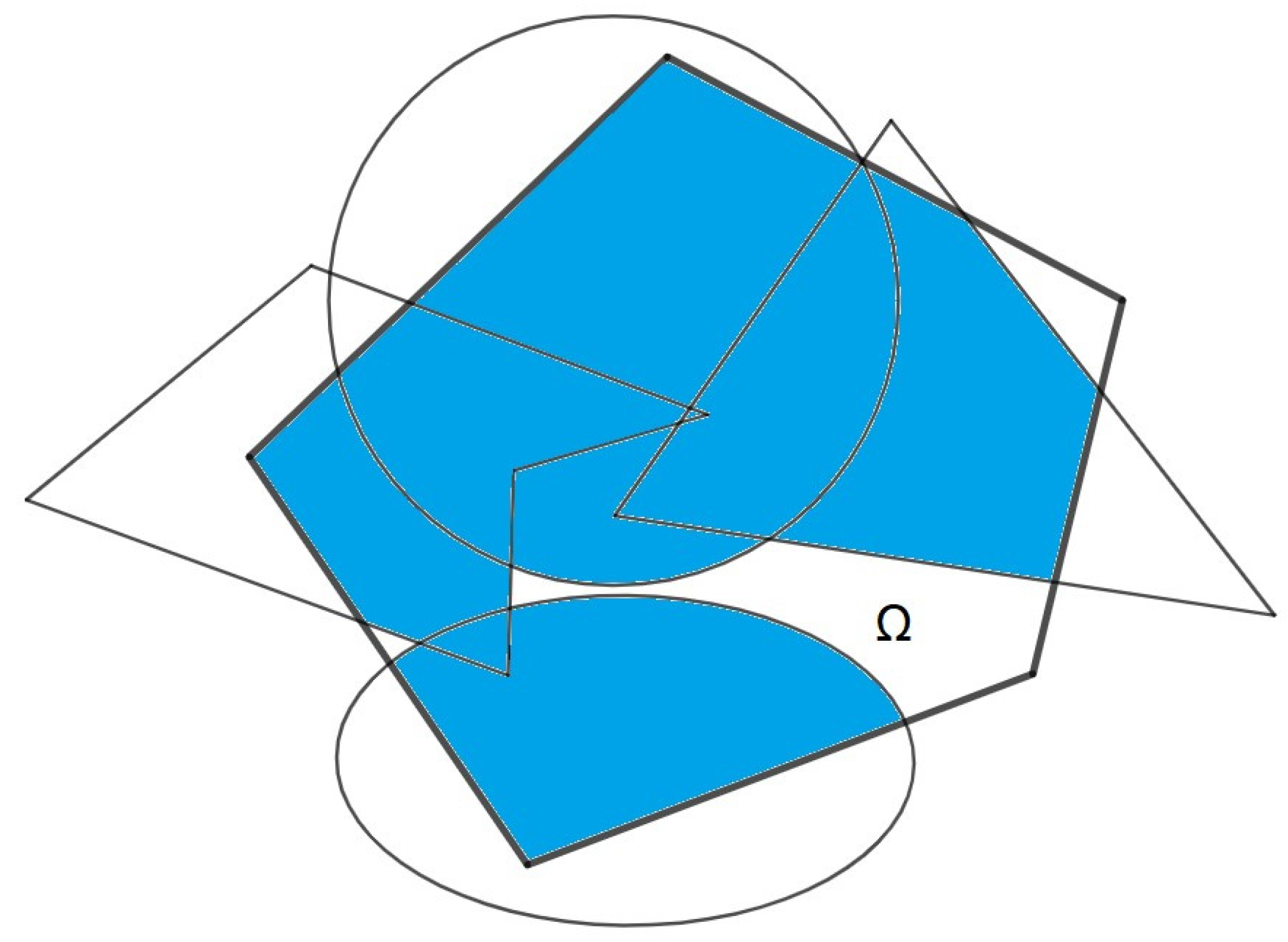
Consider a demand region, $\Omega$, and a family of facilities (service areas), ${\mathrm{S}}_{\mathrm{i}},\mathrm{i}\in {\mathrm{J}}_{\mathrm{n}}$. The set ${\mathrm{J}}_{\mathrm{n}}=\left\{1,\dots ,\mathrm{n}\right\}$ will be referred to as the index set. The objective is to determine the placement of service areas ${\mathrm{S}}_{\mathrm{i}},\mathrm{i}\in {\mathrm{J}}_{\mathrm{n}}$ with respect to demand region $\Omega$ to optimize a given criterion. The specifics of this problem depend on the choice of the objective function, the characteristics of the service areas, and the constraints on their location. In this study, both $\Omega$ and ${\mathrm{S}}_{\mathrm{i}},\mathrm{i}\in {\mathrm{J}}_{\mathrm{n}}$ are considered planar geometric facilities in the Euclidean plane, ${\mathrm{E}}^2$. The objective function is defined as the area of region $\Omega$ covered by service areas ${\mathrm{S}}_{\mathrm{i}},\mathrm{i}\in {\mathrm{J}}_{\mathrm{n}}$, which is to be maximized.

Figure 1 illustrates a portion of demand region $\Omega$ that is covered by four service areas: a non-convex polygon, a triangle, a circle, and an ellipse.

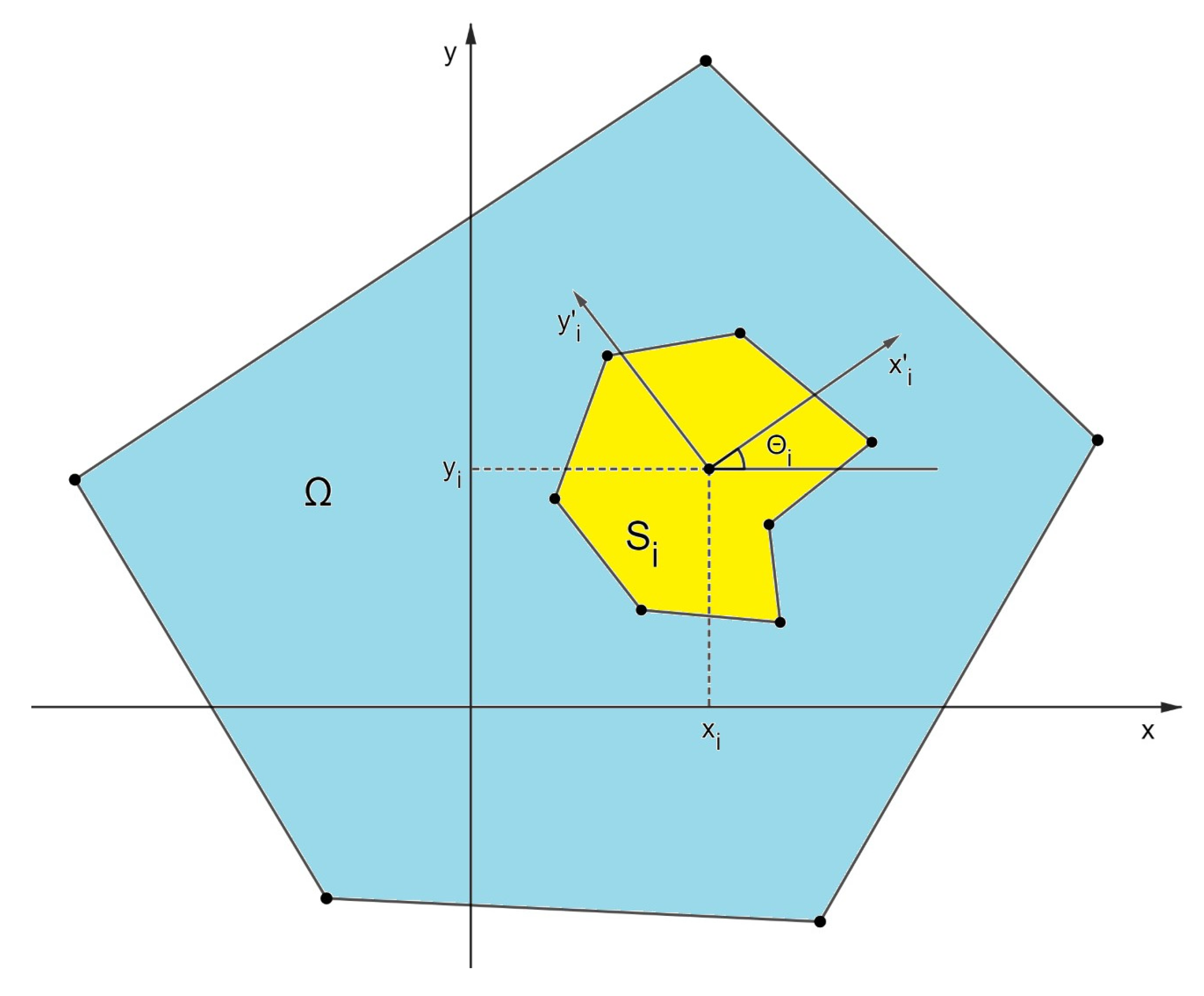
Let $\mathrm{O}\mathrm{x}\mathrm{y}$ denote a Cartesian coordinate system in the Euclidean plane, ${\mathrm{E}}^2$. The position of demand region $\Omega$ is fixed within this system. For each service area, ${\mathrm{S}}_{\mathrm{i}}$, an internal reference, ${\mathrm{c}}_{\mathrm{i}},\mathrm{i}\in {\mathrm{J}}_{\mathrm{n}}$, is specified, referred to as its pole. The location of ${\mathrm{S}}_{\mathrm{i}}$ is determined by the coordinates $({\mathrm{x}}_{\mathrm{i}},{\mathrm{y}}_{\mathrm{i}})$ of the pole, ${\mathrm{c}}_{\mathrm{i}}$, and the angle, ${\mathsf{\theta }}_{\mathrm{i}}$, of rotation with respect to the $\mathrm{O}\mathrm{x}\mathrm{y}$ coordinate system (Figure 2). We define ${\mathrm{p}}^{\mathrm{i}}=({\mathrm{x}}_{\mathrm{i}},{\mathrm{y}}_{\mathrm{i}},{\mathsf{\theta }}_{\mathrm{i}})$ as the placement parameters of ${\mathrm{S}}_{\mathrm{i}}$. A service area, ${\mathrm{S}}_{\mathrm{i}}$, with placement parameters, ${\mathrm{p}}^{\mathrm{i}}$, will be denoted as ${\mathrm{S}}_{\mathrm{i}}({\mathrm{p}}^{\mathrm{i}})$ and referred to as a parameterized facility.

Let us define a parameterized complex facility as

$$\mathrm{S}(\mathbf{p})=\Omega \cap {\displaystyle \underset{\mathrm{i}=1}{\overset{\mathrm{n}}{\cup }}{\mathrm{S}}_{\mathrm{i}}}({\mathrm{p}}^{\mathrm{i}}),$$

(1)

where $\mathbf{p}=({\mathrm{p}}^1,\dots ,{\mathrm{p}}^{\mathrm{n}})$.

We introduce the characteristic function,

$${\mathsf{\lambda }}_{\mathrm{i}}(\mathrm{P},{\mathrm{p}}^{\mathrm{i}})=\hspace{0.17em}\{\begin{array}{l}1,\hspace{0.17em}\mathrm{i}\mathrm{f}\hspace{0.17em}\mathrm{P}\in {\mathrm{S}}_{\mathrm{i}}({\mathrm{p}}^{\mathrm{i}});\\ 0,\hspace{0.17em}\mathrm{i}\mathrm{f}\hspace{0.17em}\mathrm{P}\notin {\mathrm{S}}_{\mathrm{i}}({\mathrm{p}}^{\mathrm{i}}),\end{array}$$

where $\mathrm{P}=(\mathrm{x},\mathrm{y})\in {\mathrm{E}}^2$.

Then, the function

$$\mathsf{\mu }(\mathbf{p})={\displaystyle \underset{\Omega }{\iint }\left(1-{\displaystyle \prod _{\mathrm{i}=1}^{\mathrm{n}}\left(1-{\mathsf{\lambda }}_{\mathrm{i}}(\mathrm{P},{\mathrm{p}}^{\mathrm{i}})\right)}\right)}\mathrm{d}\mathrm{x}\mathrm{d}\mathrm{y}$$

(2)

defines the dependence of the area of the parameterized complex facility, $\mathrm{S}(\mathbf{p})$, on the placement parameters, $\mathbf{p}=({\mathrm{p}}^1,\dots ,{\mathrm{p}}^{\mathrm{n}})$.

Thus, the continuous maximum coverage location problem, in general, can be formulated as follows:

$$\mathsf{\mu }(\mathbf{p})\to \max$$

(3)

subject to

$$\mathbf{p}\in \mathrm{D},$$

(4)

where $\mathrm{D}$ is the feasible domain of the placement parameters, $\mathbf{p}=({\mathrm{p}}^1,\dots ,{\mathrm{p}}^{\mathrm{n}})$.

The solution to such a problem is significantly more complex due to its high dimensionality and multi-extremal nature. This complexity underscores the need to develop specialized optimization methods that account for the unique characteristics of the objective function (2). We propose an approach that combines local and global optimization methods. At the local optimization stage, we leverage specific properties of the objective function, $\mathsf{\mu }(\mathbf{p})$, derived from geometric considerations.

It is important to note that the choice of a local optimization method also depends on the properties of the feasible domain, $\mathrm{D}$. In this study, we focus on the CMCLP with and without constraints on the placement parameters, emphasizing the analysis of the objective function’s properties.

3. Local Optimization Stage for CMCLP

Let us now consider the features of the local optimization stage. Specifying the objective function, $\mathsf{\mu }(\mathbf{p})$, analytically as a function of the placement parameters, $\mathbf{p}=({\mathrm{p}}^1,\dots ,{\mathrm{p}}^{\mathrm{n}})$, presents significant challenges. This task is extremely difficult, even for simple shapes, such as circular demand region $\Omega$ and the service areas, ${\mathrm{S}}_{\mathrm{i}},\mathrm{i}\in {\mathrm{J}}_{\mathrm{n}}$.

However, we can use computational geometry libraries for calculations, $\mathsf{\mu }(\widehat{\mathbf{p}})$, at fixed values of the placement parameters, $\widehat{\mathbf{p}}=({\widehat{\mathrm{p}}}^1,\dots ,{\widehat{\mathrm{p}}}^{\mathrm{n}})$. An example is the Python Shapely library [21], which allows for operations on geometric facilities using Boolean operators. This package enables the construction of complex geometric facilities from basic shapes, such as polygons, circles, and ellipses.

Importantly, the area of the complex geometric facility,

$$\mathrm{S}(\widehat{\mathbf{p}})=\Omega \cap {\displaystyle \underset{\mathrm{i}=1}{\overset{\mathrm{n}}{\cup }}{\mathrm{S}}_{\mathrm{i}}}({\widehat{\mathrm{p}}}^{\mathrm{i}})$$

(5)

formed by unions and intersections of irregular polygons, circles, and ellipses can be automatically calculated using this library. Python code for these calculations is provided in [22,23].

Thus, to search for the local extrema of the function $\mathsf{\mu }(\mathbf{p})$, gradient-based local optimization methods using first-order differences can be applied. On the one hand, the computational time for finding a local extremum depends on the proximity of the starting point to the actual extremum. Thus, it is important to form sufficiently good initial approximations. On the other hand, we are interested in estimating the area of a complex facility, $\mathrm{S}(\widehat{\mathbf{p}})$, without having to perform union operations on all of the individual facilities, ${\mathrm{S}}_{\mathrm{i}}({\widehat{\mathrm{p}}}^{\mathrm{i}}),\mathrm{i}\in {\mathrm{J}}_{\mathrm{n}}$, that comprise it.

To solve the approximation problem, we propose an approach based on the following property of the function $\mathsf{\mu }(\mathbf{p})$. For fixed placement parameters, $\widehat{\mathbf{p}}=({\widehat{\mathrm{p}}}^1,\dots ,{\widehat{\mathrm{p}}}^{\mathrm{n}})$, we can apply the Inclusion–Exclusion Principle to express the following:

$$\begin{gathered} \begin{array}{l}\mathit{mes}\left(\mathrm{S}(\widehat{\mathbf{p}})\right)=\mathit{mes}\left({\displaystyle \underset{\mathrm{i}=1}{\overset{\mathrm{n}}{\cup }}\left(\Omega \cap {\mathrm{S}}_{\mathrm{i}}({\widehat{\mathrm{p}}}^{\mathrm{i}})\right)}\right)=\\ ={\displaystyle \sum _{\mathrm{i}}\mathit{mes}\left(\Omega \cap {\mathrm{S}}_{\mathrm{i}}({\widehat{\mathrm{p}}}^{\mathrm{i}})\right)}-{\displaystyle \sum _{\mathrm{i}<\mathrm{j}}\mathit{mes}\left(\Omega \cap {\mathrm{S}}_{\mathrm{i}}({\widehat{\mathrm{p}}}^{\mathrm{i}})\cap {\mathrm{S}}_{\mathrm{j}}({\widehat{\mathrm{p}}}^{\mathrm{j}})\right)+}\end{array} \\ \begin{array}{l}+{\displaystyle \sum _{\mathrm{i}<\mathrm{j}<\mathrm{k}}\mathit{mes}\left(\Omega \cap {\mathrm{S}}_{\mathrm{i}}({\widehat{\mathrm{p}}}^{\mathrm{i}})\cap {\mathrm{S}}_{\mathrm{j}}({\widehat{\mathrm{p}}}^{\mathrm{j}})\cap {\mathrm{S}}_{\mathrm{k}}({\widehat{\mathrm{p}}}^{\mathrm{k}})\right)+\dots }\\ +{(-1)}^{\mathrm{n}-1}\mathit{mes}\left(\Omega \cap {\mathrm{S}}_1({\widehat{\mathrm{p}}}^1)\cap {\mathrm{S}}_2({\widehat{\mathrm{p}}}^2)\cap \dots \cap {\mathrm{S}}_{\mathrm{n}}({\widehat{\mathrm{p}}}^{\mathrm{n}})\right)\end{array}, \end{gathered}$$

(6)

where $\mathit{mes}\left(\mathrm{S}\right)$ defines the area of the set, $\mathrm{S}$.

By limiting the number of terms in the series (6), i.e., the number of facility overlaps, ${\mathrm{S}}_{\mathrm{i}}({\widehat{\mathrm{p}}}^{\mathrm{i}}),\mathrm{i}\in {\mathrm{J}}_{\mathrm{n}}$, we can estimate the area of the complex facility, $\mathrm{S}(\widehat{\mathbf{p}})$, significantly reducing computational costs. This approach is well suited for solving the continuous maximum coverage location problem with arbitrarily shaped facilities. Indeed, it is reasonable to expect that, when maximizing the function $\mathsf{\mu }(\mathbf{p})$, the multiplicity of facility overlaps will decrease.

4. Elastic Modeling Approach

Let us consider the following functions:

$${\mathsf{\mu }}_{\mathrm{i}0}({\mathrm{p}}^{\mathrm{i}})={\displaystyle \underset{\Omega }{\iint }{\mathsf{\lambda }}_{\mathrm{i}}(\mathrm{P},{\mathrm{p}}^{\mathrm{i}})}\mathrm{d}\mathrm{x}\mathrm{d}\mathrm{y}$$

(7)

$${\mathsf{\mu }}_{\mathrm{i}\mathrm{j}}({\mathrm{p}}^{\mathrm{i}},{\mathrm{p}}^{\mathrm{j}})={\displaystyle \iint {\mathsf{\lambda }}_{\mathrm{i}}(\mathrm{P},{\mathrm{p}}^{\mathrm{i}}){\mathsf{\lambda }}_{\mathrm{j}}(\mathrm{P},{\mathrm{p}}^{\mathrm{j}})}\mathrm{d}\mathrm{x}\mathrm{d}\mathrm{y}$$

(8)

Formula (7) defines the dependence of the overlapping area between a parameterized facility, ${\mathrm{S}}_{\mathrm{i}}({\mathrm{p}}^{\mathrm{i}})$, and region $\Omega$ on the placement parameters, ${\mathrm{p}}^{\mathrm{i}}$. Formula (8) determines the dependence of the overlapping area of the parameterized facilities, ${\mathrm{S}}_{\mathrm{i}}({\mathrm{p}}^{\mathrm{i}})$ and ${\mathrm{S}}_{\mathrm{i}}({\mathrm{p}}^{\mathrm{i}})$, on their placement parameters, ${\mathrm{p}}^{\mathrm{i}}$ and ${\mathrm{p}}^{\mathrm{j}}$.

We then define the function:

$$\tilde{\mathsf{\mu }}(\mathbf{p})={\displaystyle \sum _{\mathrm{i}=1}^{\mathrm{n}}{\mathsf{\mu }}_{\mathrm{i}0}({\mathrm{p}}^{\mathrm{i}})}-{\displaystyle \sum _{\mathrm{i}=1}^{\mathrm{n}-1}{\displaystyle \sum _{\mathrm{j}=\mathrm{i}+1}^{\mathrm{n}}{\mathsf{\mu }}_{\mathrm{i}\mathrm{j}}}}({\mathrm{p}}^{\mathrm{i}},{\mathrm{p}}^{\mathrm{j}})$$

(9)

According to Formula (6), the function $\tilde{\mathsf{\mu }}(\mathbf{p})$ serves as an approximation of $\mathsf{\mu }(\mathbf{p})$ when we restrict our analysis to double-overlapping regions and disregard higher-order overlaps.

Thus, the following optimization problem can be formulated:

$$\tilde{\mathsf{\mu }}(\mathbf{p})\to \mathit{max},$$

(10)

Solving Problem (10) provides an approximate solution to the unconstrained optimization problem (3). The primary advantage of Model (10) lies in its significant reduction in computational complexity compared to directly calculating $\mathsf{\mu }(\mathbf{p})$ at fixed placement parameters. Indeed, computing the overlapping area of two objects is much simpler than calculating the area of a complex facility, $\mathrm{S}(\widehat{\mathbf{p}})$, as defined in Formula (5). This simplification is particularly critical when employing gradient-based optimization methods with first-order differences.

We refer to Model (10) with the objective function of Formula (9) as the extended elastic model [24] for Problem (3). The term “elastic” is used because the model is a generalization of the well-known elastic (quasi-physical, quasi-human) model [25,26,27] applied to the Circle Packing Problem [28,29].

Consider the Circle Packing Problem, formulated as follows. Given a circular container, $\Omega$, with an undetermined radius, $\mathrm{R}$, as well as n circles, ${\mathrm{S}}_{\mathrm{i}},\mathrm{i}\in {\mathrm{J}}_{\mathrm{n}}$, with known radii, ${\mathrm{r}}_{\mathrm{i}},\mathrm{i}\in {\mathrm{J}}_{\mathrm{n}}$, let the center of $\Omega$ be the origin of the two-dimensional coordinate system, and let the coordinate of the center of ${\mathrm{S}}_{\mathrm{i}}$ be ${\mathrm{p}}^{\mathrm{i}}=({\mathrm{x}}_{\mathrm{i}},{\mathrm{y}}_{\mathrm{i}})$. The problem is to find a feasible placement (non-overlapping and not exceeding the container) with the smallest container radius, $\mathrm{R}$.

The objective can be formulated below:

$$\mathrm{R}\to \mathit{min}$$

(11)

subject to

$${\mathrm{d}}_{\mathrm{i}0}\le \mathrm{R}-{\mathrm{r}}_{\mathrm{i}},\hspace{0.17em}\mathrm{i}\in {\mathrm{J}}_{\mathrm{n}},$$

(12)

$${\mathrm{d}}_{\mathrm{i}\mathrm{j}}\ge {\mathrm{r}}_{\mathrm{i}}+{\mathrm{r}}_{\mathrm{j}},\hspace{0.17em}\mathrm{i},\mathrm{j}\in {\mathrm{J}}_{\mathrm{n}},\hspace{0.17em}\mathrm{j}>\mathrm{i},$$

(13)

where

$${\mathrm{d}}_{\mathrm{i}0}=\sqrt{{\mathrm{x}}_{\mathrm{i}}^2+{\mathrm{y}}_{\mathrm{i}}^2}$$

$${\mathrm{d}}_{\mathrm{i}\mathrm{j}}=\sqrt{{({\mathrm{x}}_{\mathrm{i}}-{\mathrm{y}}_{\mathrm{i}})}^2+{({\mathrm{x}}_{\mathrm{j}}-{\mathrm{y}}_{\mathrm{j}})}^2}.$$

The elastic model of Problems (11)–(13) is based on its relaxation, assuming that the objects are elastic and their overlapping and extension beyond the container is allowed. The degree of overlap between facilities is determined by the so-called function extrusion elastic potential energy, which has the form

$$\mathrm{E}({\mathrm{p}}^1,\dots ,{\mathrm{p}}^{\mathrm{n}})={\displaystyle \sum _{\mathrm{i}=1}^{\mathrm{n}}{\mathrm{E}}_{\mathrm{i}0}({\mathrm{p}}^{\mathrm{i}})}+{\displaystyle \sum _{\mathrm{i}=1}^{\mathrm{n}-1}{\displaystyle \sum _{\mathrm{j}=\mathrm{i}+1}^{\mathrm{n}}{\mathrm{E}}_{\mathrm{i}\mathrm{j}}({\mathrm{p}}^{\mathrm{i}},{\mathrm{p}}^{\mathrm{j}})}},$$

(14)

where

$${\mathrm{E}}_{\mathrm{i}0}({\mathrm{p}}^{\mathrm{i}})=ma{x}^2\left\{0,\hspace{0.17em}\mathrm{R}-{\mathrm{r}}_{\mathrm{i}}-{\mathrm{d}}_{\mathrm{i}0}\right\}$$

(15)

$${\mathrm{E}}_{\mathrm{i}\mathrm{j}}({\mathrm{p}}^{\mathrm{i}},{\mathrm{p}}^{\mathrm{j}})=ma{x}^2\left\{0,\hspace{0.17em}{\mathrm{r}}_{\mathrm{i}}+{\mathrm{r}}_{\mathrm{j}}-\hspace{0.17em}{\mathrm{d}}_{\mathrm{i}\mathrm{j}}\right\}.$$

(16)

Squaring function max in Formulas (15) and (16) ensures the non-negativity and differentiability of the function $\mathrm{E}({\mathrm{p}}^1,\dots ,{\mathrm{p}}^{\mathrm{n}})$.

As a result, we arrive at the following nonlinear optimization problem:

$$\mathrm{E}({\mathrm{p}}^1,\dots ,{\mathrm{p}}^{\mathrm{n}})\to \mathit{min}.$$

(17)

This problem is treated as an auxiliary problem when solving Problems (11)–(13), particularly when using the penalty function method.

Unfortunately, extending the elastic model ((15)–(17)) to the packing problem with irregular facilities presents challenges due to the difficulty in determining the distances between them. One possible solution is to use the phi-function method [30,31]. However, well-known analytical formulas for phi-functions are primarily designed for positive values [32,33]. For overlapping facilities, the corresponding phi-functions must be negative, adding complexity to the problem.

For the packing problem with arbitrarily shaped facilities, we propose using the extended elastic model, assuming that

$${\mathrm{E}}_{\mathrm{i}0}({\mathrm{p}}^{\mathrm{i}})=\mathit{mes}\left({\mathrm{S}}_{\mathrm{i}}\right)-{\mathsf{\mu }}_{\mathrm{i}0}({\mathrm{p}}^{\mathrm{i}})$$

$${\mathrm{E}}_{\mathrm{i}\mathrm{j}}({\mathrm{p}}^{\mathrm{i}},{\mathrm{p}}^{\mathrm{j}})={\mathsf{\mu }}_{\mathrm{i}\mathrm{j}}({\mathrm{p}}^{\mathrm{i}},{\mathrm{p}}^{\mathrm{j}}),$$

where the functions ${\mathsf{\mu }}_{\mathrm{i}0}({\mathrm{p}}^{\mathrm{i}})$ and ${\mathsf{\mu }}_{\mathrm{i}\mathrm{j}}({\mathrm{p}}^{\mathrm{i}},{\mathrm{p}}^{\mathrm{j}})$ are provided by Formulas (7) and (8), respectively.

Let ${\mathrm{r}}_1\le {\mathrm{r}}_2\le \dots \le {\mathrm{r}}_{\mathrm{n}}<\mathrm{R}$. Then, for $\mathrm{i},\mathrm{j}\in {\mathrm{J}}_{\mathrm{n}},\hspace{0.17em}\mathrm{j}>\mathrm{i}$, we have

$$\begin{gathered} {\mathsf{\mu }}_{\mathrm{i}\mathrm{j}}({\mathrm{p}}^{\mathrm{i}},{\mathrm{p}}^{\mathrm{j}})=0 \mathrm{if} {\mathrm{d}}_{\mathrm{i}\mathrm{j}}\ge {\mathrm{r}}_{\mathrm{i}}+{\mathrm{r}}_{\mathrm{j}}; \\ {\mathsf{\mu }}_{\mathrm{i}\mathrm{j}}({\mathrm{p}}^{\mathrm{i}},{\mathrm{p}}^{\mathrm{j}})=\mathsf{\pi }{\mathrm{r}}_{\mathrm{i}}^2 \mathrm{if} {\mathrm{d}}_{\mathrm{i}\mathrm{j}}\le {\mathrm{r}}_{\mathrm{j}}-{\mathrm{r}}_{\mathrm{i}}; \\ {\mathsf{\mu }}_{\mathrm{i}0}({\mathrm{p}}^{\mathrm{i}})=0 \mathrm{if} {\mathrm{d}}_{\mathrm{i}0}\ge \mathrm{R}+{\mathrm{r}}_{\mathrm{i}} \\ {\mathsf{\mu }}_{\mathrm{i}0}({\mathrm{p}}^{\mathrm{i}},{\mathrm{p}}^0)=\mathsf{\pi }{\mathrm{r}}_{\mathrm{i}}^2 \mathrm{if} {\mathrm{d}}_{\mathrm{i}0}\le \mathrm{R}-{\mathrm{r}}_{\mathrm{i}}. \end{gathered}$$

If ${\mathrm{r}}_{\mathrm{j}}-{\mathrm{r}}_{\mathrm{i}}<{\mathrm{d}}_{\mathrm{i}\mathrm{j}}<{\mathrm{r}}_{\mathrm{i}}+{\mathrm{r}}_{\mathrm{j}}$ or $\mathrm{R}-{\mathrm{r}}_{\mathrm{i}}<{\mathrm{d}}_{\mathrm{i}0}<\mathrm{R}+{\mathrm{r}}_{\mathrm{i}}$, we can write

$$\begin{gathered} {\mathsf{\mu }}_{\mathrm{i}0}({\mathrm{p}}^{\mathrm{i}})={\mathrm{r}}_{\mathrm{i}}^{2}arccos{\displaystyle \frac{{\mathrm{R}}^2-{\mathrm{r}}_{\mathrm{i}}^2+{\mathrm{d}}_{\mathrm{i}0}^2}{2\hspace{0.17em}{\mathrm{r}}_{\mathrm{i}}\hspace{0.17em}{\mathrm{d}}_{\mathrm{i}0}}}-{\displaystyle \frac{{\mathrm{R}}^2-{\mathrm{r}}_{\mathrm{i}}^2+{\mathrm{d}}_{\mathrm{i}0}^2}{2\hspace{0.17em}{\mathrm{d}}_{\mathrm{i}0}\hspace{0.17em}}}\hspace{0.17em}\sqrt{{\mathrm{r}}_{\mathrm{i}}^2-{\displaystyle \frac{{\left({\mathrm{R}}^2-{\mathrm{r}}_{\mathrm{i}}^2+{\mathrm{d}}_{\mathrm{i}0}^2\right)}^2}{4{\mathrm{d}}_{\mathrm{i}0}^2}}}+ \\ +{\mathrm{R}}^{2}arccos{\displaystyle \frac{{\mathrm{r}}_{\mathrm{i}}^2-{\mathrm{R}}^2+{\mathrm{d}}_{\mathrm{i}0}^2}{2\hspace{0.17em}\mathrm{R}\hspace{0.17em}{\mathrm{d}}_{\mathrm{i}0}}}-{\displaystyle \frac{{\mathrm{r}}_{\mathrm{i}}^2-{\mathrm{R}}^2+{\mathrm{d}}_{\mathrm{i}0}^2}{2\hspace{0.17em}{\mathrm{d}}_{\mathrm{i}0}\hspace{0.17em}}}\hspace{0.17em}\sqrt{{\mathrm{R}}^2-{\displaystyle \frac{{\left({\mathrm{r}}_{\mathrm{i}}^2-{\mathrm{R}}^2+{\mathrm{d}}_{\mathrm{i}0}^2\right)}^2}{4{\mathrm{d}}_{\mathrm{i}0}^2}}} \end{gathered}$$

(18)

$$\begin{gathered} {\mathsf{\mu }}_{\mathrm{i}\mathrm{j}}({\mathrm{p}}^{\mathrm{i}},{\mathrm{p}}^{\mathrm{j}})={\mathrm{r}}_{\mathrm{j}}^{2}arccos{\displaystyle \frac{{\mathrm{r}}_{\mathrm{j}}^2-{\mathrm{r}}_{\mathrm{i}}^2+{\mathrm{d}}_{\mathrm{i}\mathrm{j}}^2}{2\hspace{0.17em}{\mathrm{r}}_{\mathrm{j}}\hspace{0.17em}{\mathrm{d}}_{\mathrm{i}\mathrm{j}}}}-{\displaystyle \frac{{\mathrm{r}}_{\mathrm{j}}^2-{\mathrm{r}}_{\mathrm{i}}^2+{\mathrm{d}}_{\mathrm{i}\mathrm{j}}^2}{2\hspace{0.17em}{\mathrm{d}}_{\mathrm{i}\mathrm{j}}\hspace{0.17em}}}\hspace{0.17em}\sqrt{{\mathrm{r}}_{\mathrm{j}}^2-{\displaystyle \frac{{\left({\mathrm{r}}_{\mathrm{j}}^2-{\mathrm{r}}_{\mathrm{i}}^2+{\mathrm{d}}_{\mathrm{i}\mathrm{j}}^2\right)}^2}{4{\mathrm{d}}_{\mathrm{i}\mathrm{j}}^2}}}+ \\ +{\mathrm{r}}_{\mathrm{i}}^{2}arccos{\displaystyle \frac{{\mathrm{r}}_{\mathrm{i}}^2-{\mathrm{r}}_{\mathrm{j}}^2+{\mathrm{d}}_{\mathrm{i}\mathrm{j}}^2}{2\hspace{0.17em}{\mathrm{r}}_{\mathrm{i}}\hspace{0.17em}{\mathrm{d}}_{\mathrm{i}\mathrm{j}}}}-{\displaystyle \frac{{\mathrm{r}}_{\mathrm{i}}^2-{\mathrm{r}}_{\mathrm{j}}^2+{\mathrm{d}}_{\mathrm{i}\mathrm{j}}^2}{2\hspace{0.17em}{\mathrm{d}}_{\mathrm{i}\mathrm{j}}\hspace{0.17em}}}\hspace{0.17em}\sqrt{{\mathrm{r}}_{\mathrm{i}}^2-{\displaystyle \frac{{\left({\mathrm{r}}_{\mathrm{i}}^2-{\mathrm{r}}_{\mathrm{j}}^2+{\mathrm{d}}_{\mathrm{i}\mathrm{j}}^2\right)}^2}{4{\mathrm{d}}_{\mathrm{i}\mathrm{j}}^2}}}, \end{gathered}$$

(19)

Note that Formulas (18) and (19) are more complex than (15) and (16), but the question of how much better the packing of circles will be achieved by using them in Problem (17) remains open. This issue falls outside the scope of our study, as it is more closely related to the packing problem.

In the context of the CMCLP, the coverage area of region $\Omega$ plays a crucial role, which limits the applicability of the elastic model ((14)–(17)). However, the use of the extended elastic model is justified for both the packing and coverage problems with arbitrarily shaped objects. In this case, Formulas (18) and (19) are valuable, as they enable the calculation of the overlapping area of circular facilities.

It is worth mentioning that formulas for the overlapping area of ellipses are also known, but we do not present them here due to their complexity. For two ellipses, the overlapping area is determined by adding the areas of the corresponding sectors and polygons. The intersection points of two general ellipses are found using Ferrari’s quartic formula, which solves the polynomial resulting from combining the equations of the two ellipses.

5. Numerical Experiments

In this section, we provide a numerical justification for using the extended elastic model in the CMCLP. A series of numerical experiments were conducted to substantiate the feasibility of applying Model (10) for estimating local solutions to Problem (3). We will consider the CMCLP both an unconstrained and constrained optimization problem. The following computer configuration was used for the experiments: Intel Core i7-5557U processor (3.1 GHz, 2 cores, 4 threads), 16 GB DDR3 1866 MHz RAM, Intel Iris Graphics 6100 GPU with 1.5 GB of video memory, and a 512 GB SSD, running macOS 11.0 Big Sur.

For calculations, we used Python libraries. Specifically, Shapely was employed to perform logical operations on geometric objects and to determine the areas of the resulting complex objects, while scipy.optimize was utilized for the local optimization of the functions $\mathsf{\mu }(\mathbf{p})$ and $\tilde{\mathsf{\mu }}(\mathbf{p})$.

5.1. Solving Unconstrained Problem Using Extended Elastic Model

Let us analyze how closely the local solutions of unconstrained Problems (3) and (10) align in terms of the objective function value when using the same optimization method and starting point. For testing, demand region $\Omega$ was modeled as an irregular polygon, and for the service areas, ${\mathrm{S}}_{\mathrm{i}},\mathrm{i}\in {\mathrm{J}}_{\mathrm{n}}$, n = 50 were arbitrary shapes. These included 30 polygons with vertex counts ranging from three to eight, as well as 10 circles and 10 ellipses. The vertex coordinates for region $\Omega$ and polygons ${\mathrm{S}}_{\mathrm{i}},\mathrm{i}\in {\mathrm{J}}_{30}$ are presented in

Table 1. Vertex coordinates of polygonal demand region $\Omega$.

i	1	2	3	4	5	6	7
${\mathrm{x}}_{\mathrm{i}}$	−60	−70	−210	−170	−40	180	200
${\mathrm{y}}_{\mathrm{i}}$	−175	−145	0	170	90	210	−20

and

Table 2. Vertex coordinates of polygonal service areas ${\mathrm{S}}_1–{\mathrm{S}}_{30}$.

	${\mathrm{x}}_1$	${\mathrm{y}}_1$	${\mathrm{x}}_2$	${\mathrm{y}}_2$	${\mathrm{x}}_3$	${\mathrm{y}}_3$	${\mathrm{x}}_4$	${\mathrm{y}}_4$	${\mathrm{x}}_5$	${\mathrm{y}}_5$	${\mathrm{x}}_6$	${\mathrm{y}}_6$	${\mathrm{x}}_7$	${\mathrm{y}}_7$	${\mathrm{x}}_8$	${\mathrm{y}}_8$	Area
${\mathrm{S}}_1$	12	0	−10	18	−11	−20											427
${\mathrm{S}}_2$	35	0	−17	29	−18	−31											1574.5
${\mathrm{S}}_3$	40	0	−12	40	−18	−38											2148
${\mathrm{S}}_4$	20	10	−15	26	−16	−28											953
${\mathrm{S}}_5$	31	0	−15	26	−18	−31											1350
${\mathrm{S}}_6$	24	0	0	23	−30	0	0	−22									1215
${\mathrm{S}}_7$	20	0	0	10	−22	0	0	−17									567
${\mathrm{S}}_8$	34	0	0	30	−25	0	0	−40									2065
${\mathrm{S}}_9$	40	0	0	30	−40	0	0	−35									2600
${\mathrm{S}}_{10}$	20	0	0	20	−25	0	0	−25									1012.5
${\mathrm{S}}_{11}$	17	0	11	35	−22	16	−24	−18	10	−28							1824.5
${\mathrm{S}}_{12}$	30	0	5	16	−18	13	−19	−14	8	−25							1334.5
${\mathrm{S}}_{13}$	15	−10	9	19	−25	8	−16	−21	0	−10							942.5
${\mathrm{S}}_{14}$	16	0	5	20	−13	10	−19	−13	2	−27							980
${\mathrm{S}}_{15}$	20	0	7	23	−12	9	−20	−14	5	−16							928.5
${\mathrm{S}}_{16}$	40	10	13	13	−3	33	−30	10	−11	−27	28	−22					2448
${\mathrm{S}}_{17}$	40	0	14	24	−20	20	−40	0	−1	−7	22	−37					2235.5
${\mathrm{S}}_{18}$	31	0	23	40.38	−18	31	−22	0	−13	−23	19	−33					2884.31
${\mathrm{S}}_{19}$	28	0.	11	19	−15	27	−35	0	−17	−30	13	−23					2267
${\mathrm{S}}_{20}$	10	0	26	28	0	22	−23	0	0	−16	20	−14					1093
${\mathrm{S}}_{21}$	29	0	20	25	−7	29	−24	12	−27	−13	−6	−27	13	−17			2162.5
${\mathrm{S}}_{22}$	29	0	9	11	−4	19	−18	9	−34	−16	−4	−11	20	−25			1394.5
${\mathrm{S}}_{23}$	29	0	12	16	−5	22	−33	16	−30	−14	−3	−9	20	−25			1802
${\mathrm{S}}_{24}$	31	−10	14	18	−8	24	−24	0	−30	−5	−3	−13	11	−24			1549
${\mathrm{S}}_{25}$	23	0	11	13	−6	22	−15	7	−17	−8	−7	−27	10	−13			1104.5
${\mathrm{S}}_{26}$	14	−10	21	11	0	24	−33	24	−13	−10	−11	−21	0	−35	19	−29	1865.5
${\mathrm{S}}_{27}$	15	0	26	25	0	21	−22	21	−15	0	−18	−16	0	−33	30	−30	1986
${\mathrm{S}}_{28}$	36	10	17	27	0	18	−16	25	−29	10	−31	−19	0	−29	30	−20	2805.5
${\mathrm{S}}_{29}$	39	0	23	22	0	21	−19	19	−40	0	−30	−20	0	−28	10	−10	2405
${\mathrm{S}}_{30}$	30	0	30	30	0	30	−15	20	25	0	−25	−25	0	−34	20	−20	2752.5

, respectively. Table 2 also shows the area, $\mathit{mes}({\mathrm{S}}_{\mathrm{i}})$, of each facility, ${\mathrm{S}}_{\mathrm{i}}$. The radii of the circles and their areas are provided in

Table 3. Radii of circular service areas ${\mathrm{S}}_{31}–{\mathrm{S}}_{40}$.

i	${\mathrm{S}}_{31}$	${\mathrm{S}}_{32}$	${\mathrm{S}}_{33}$	${\mathrm{S}}_{34}$	${\mathrm{S}}_{35}$	${\mathrm{S}}_{36}$	${\mathrm{S}}_{37}$	${\mathrm{S}}_{38}$	${\mathrm{S}}_{39}$	${\mathrm{S}}_{40}$
${\mathrm{r}}_{\mathrm{i}}$	10.00	14.14	17.32	20.00	22.36	24.49	26.46	28.28	30.00	31.62
Area	314.16	628.32	942.48	1256.64	1570.8	1884.96	2199.11	2513.27	2827.43	3131.59

, and the semi-axes of the ellipses and their areas are listed in

Table 4. Semi-axes of elliptical service areas ${\mathrm{S}}_{41}–{\mathrm{S}}_{50}$.

i	${\mathrm{S}}_{41}$	${\mathrm{S}}_{42}$	${\mathrm{S}}_{43}$	${\mathrm{S}}_{44}$	${\mathrm{S}}_{45}$	${\mathrm{S}}_{46}$	${\mathrm{S}}_{47}$	${\mathrm{S}}_{48}$	${\mathrm{S}}_{49}$	${\mathrm{S}}_{50}$
${\mathrm{a}}_{\mathrm{i}}$	10.00	14.14	17.32	20.00	22.36	24.49	26.46	28.28	30.00	31.62
${\mathrm{b}}_{\mathrm{i}}$	14.14	20.00	24.49	28.28	31.62	34.64	37.42	40.00	42.43	44.72
Area	444.29	888.58	1332.86	1777.15	2221.44	2665.73	3110.02	3554.31	3998.59	4442.88

.

We specifically designed polygonal demand region $\Omega$ so that its area closely approximates the sum of the areas of objects ${\mathrm{S}}_{\mathrm{i}},\mathrm{i}\in {\mathrm{J}}_{50}$. In particular, we have

$$\mathit{mes}(\Omega )=92241.4, {\displaystyle \sum _{\mathrm{i}=1}^{50}\mathit{mes}({\mathrm{S}}_{\mathrm{i}})=92300.}$$

This approach to forming the initial data was chosen to preserve the unique characteristics of the CMCLP, which represents an intermediate formulation between the packing problem and the complete coverage problem. Specifically, given the data—such as the curvature of the object boundaries and the non-convexity of the polygons—it is neither feasible to achieve the acceptable packing of objects within the region nor to ensure its complete coverage. However, the task of maximizing the region’s coverage remains highly relevant and practical.

To validate the reliability of the results obtained using the extended elastic model, we conducted a series of experiments comparing the local solutions to unconstrained Problems (3) and (10). In these experiments, we randomly and uniformly generated the placement parameters, ${\widehat{\mathrm{p}}}^{\mathrm{i}}=({\widehat{\mathrm{x}}}_{\mathrm{i}},{\widehat{\mathrm{y}}}_{\mathrm{i}},{\widehat{\mathsf{\theta }}}_{\mathrm{i}}),\mathrm{i}\in {\mathrm{J}}_{50}$, of objects ${\mathrm{S}}_{\mathrm{i}},\mathrm{i}\in {\mathrm{J}}_{50}$, ensuring that $({\widehat{\mathrm{x}}}_{\mathrm{i}},{\widehat{\mathrm{y}}}_{\mathrm{i}})\in \Omega$ and ${\widehat{\mathsf{\theta }}}_{\mathrm{i}}\in (0,2\mathsf{\pi })$. Note that the angle parameter, ${\mathsf{\theta }}_{\mathrm{i}}$, is not required for circular objects.

To compute the overlapping area of circles and ellipses, we used known analytical expressions, specifically, Formula (19), for circular objects. The overlapping area between a polygon and other objects was calculated using the Python Shapely package.

To optimize the functions $\mathsf{\mu }(\mathbf{p})$ and $\tilde{\mathsf{\mu }}(\mathbf{p})$, starting with the starting point $\widehat{\mathbf{p}}=({\widehat{\mathrm{p}}}^1,\dots ,{\widehat{\mathrm{p}}}^{50})$, we selected the Broyden–Fletcher–Goldfarb–Shanno (BFGS) method [34], implemented via the scipy.optimize package. The BFGS method was chosen for local optimization as it offers a strong trade-off between accuracy and computational efficiency. Our choice was further supported by prior experience with this method and recommendations from researchers who have successfully applied it to packing problems. In the context of maximum coverage problems, BFGS demonstrated sufficient speed while effectively navigating local extrema.

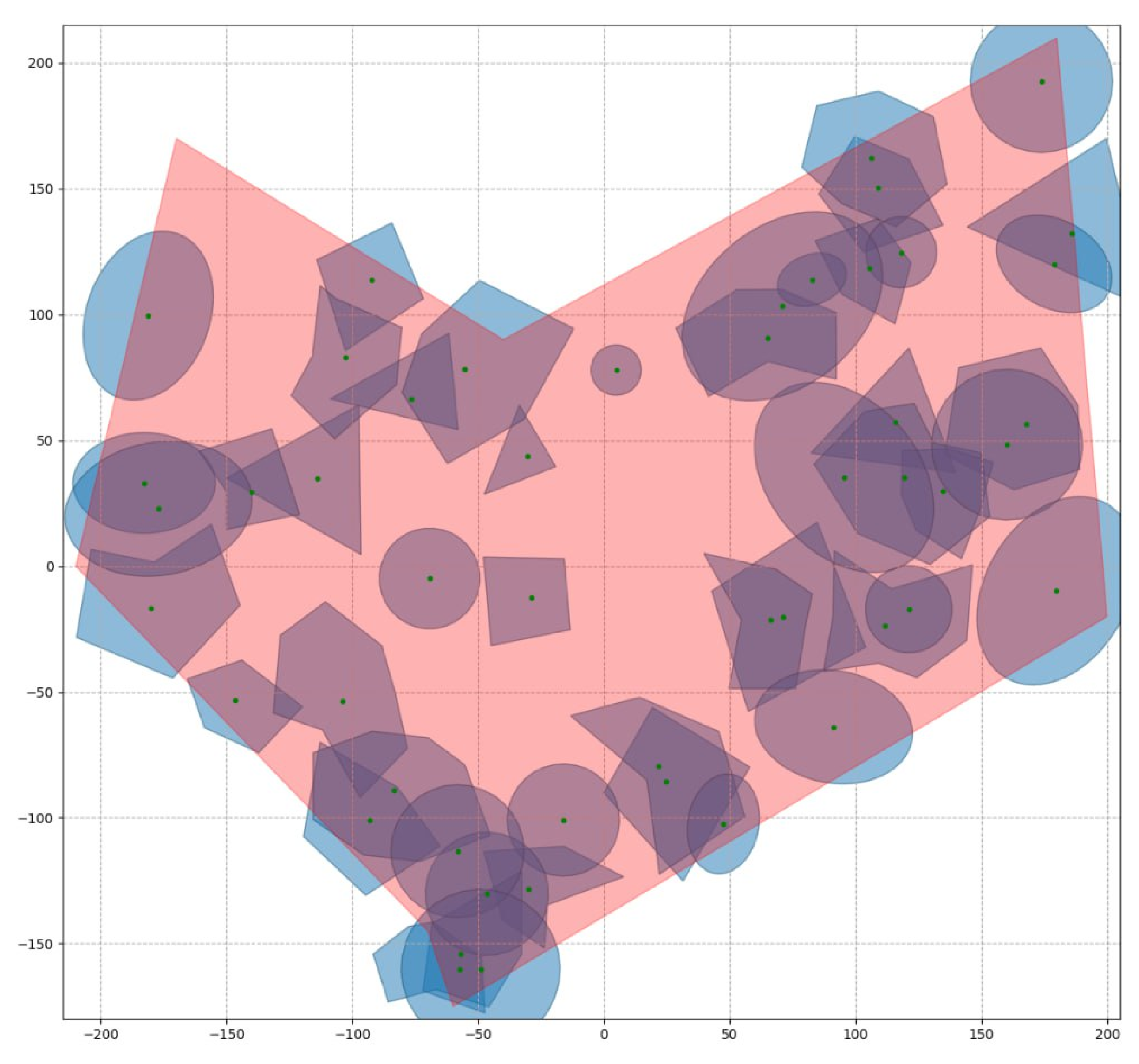
One example of a randomly chosen starting point, ${\widehat{\mathrm{p}}}^{\mathrm{i}}=({\widehat{\mathrm{x}}}_{\mathrm{i}},{\widehat{\mathrm{y}}}_{\mathrm{i}},{\widehat{\mathsf{\theta }}}_{\mathrm{i}}),\mathrm{i}\in {\mathrm{J}}_{50}$, and the corresponding initial location of objects ${\mathrm{S}}_{\mathrm{i}},\mathrm{i}\in {\mathrm{J}}_{50}$ is shown in Figure 3. In this case, the coverage area is 55,214.9. Note that in coverage problems, the quality of the solution is often characterized by the coverage density, defined as the ratio of the covered area to the total area of the region. For the initial location considered, the coverage density is 59.86%

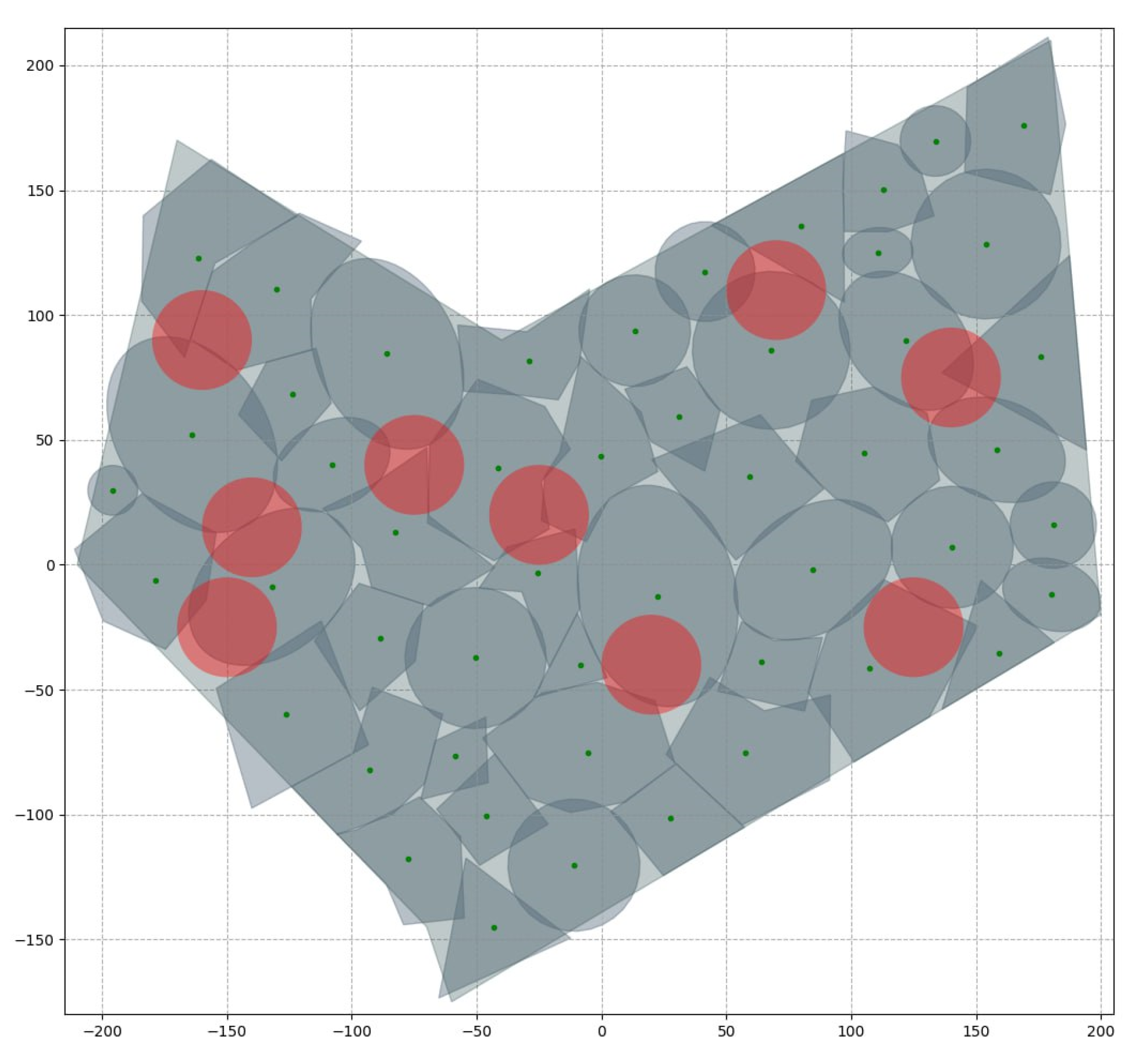
Figure 4 illustrates the placement of service areas ${\mathrm{S}}_{\mathrm{i}},\mathrm{i}\in {\mathrm{J}}_{50}$ corresponding to the local maximum of the objective function, $\tilde{\mathsf{\mu }}(\mathbf{p})$, obtained using the extended elastic model for the above starting point, $\widehat{\mathbf{p}}$. In this case, the coverage area is 86,514.2, and the coverage density increases to 94.11%. The time to find a local solution was 17 s.

Table 5. Service area placement parameters, ${\mathrm{p}}^{\mathrm{i}}=({\mathrm{x}}_{\mathrm{i}},{\mathrm{y}}_{\mathrm{i}},{\mathsf{\theta }}_{\mathrm{i}})$, for Figure 4.

i	${\mathrm{x}}_{\mathrm{i}}$	${\mathrm{y}}_{\mathrm{i}}$	${\mathsf{\theta }}_{\mathrm{i}}$	i	${\mathrm{x}}_{\mathrm{i}}$	${\mathrm{y}}_{\mathrm{i}}$	${\mathsf{\theta }}_{\mathrm{i}}$
1	−18.564	34.094	1.976	26	−106.615	−84.286	−11.049
2	−80.873	51.592	−12.765	27	112.12	−48.375	−5.636
3	134.105	112.577	16.765	28	80.431	33.54	−8.316
4	−72.346	93.564	14.508	29	−122.525	3.761	5.587
5	125.248	62.101	−37.798	30	−75.632	5.948	−8.530
6	−100.86	108.227	9.913	31	−12.636	96.258
7	−86.107	−115.210	10.955	32	104.804	91.85
8	−20.518	−85.489	4.69	33	112.787	−2.262
9	75.678	−26.266	0.647	34	−45.85	26.699
10	−30.227	−6.888	−18.98	35	−44.854	−43.755
11	−135.585	−53.698	−9.42	36	−62.461	−85.768
12	70.766	133.496	−2.013	37	−90.638	−39.248
13	−113.915	48.275	−9.978	38	158.452	172.053
14	−165.444	−31.125	13.599	39	167.89	36.872
15	93.655	72.372	−10.108	40	−44.812	−133.226
16	−181.867	2.706	1.6813	41	89.069	107.085	−23.043
17	4.558	−46.62	14.479	42	20.054	−92.481	−16.458
18	−35.035	74.641	−10.862	43	172.108	128.199	16.73
19	162.955	81.355	−13.85	44	−170.929	93.231	−2.006
20	−1.348	−125.139	−3.829	45	59.379	−80.431	12.831
21	112.247	148.266	−1.909	46	−146.032	131.658	−12.047
22	31.192	−40.256	32.981	47	−161.354	46.376	−9.008
23	28.605	50.196	−0.292	48	160.758	−14.487	−6.683
24	−132.536	83.723	1.534	49	21.932	8.349	6.965
25	123.624	27.331	6.053	50	38.462	92.43	7.499

lists the service area placement parameters, $\mathbf{p}=({\mathrm{p}}^1,\dots ,{\mathrm{p}}^{50})$, corresponding to Figure 4.

Note that there are no triple overlaps in Figure 4, meaning that $\mathsf{\mu }(\mathbf{p})=\tilde{\mathsf{\mu }}(\mathbf{p})$. Even if triple overlaps existed, the solution error (i.e., $\mathsf{\epsilon }=\left|\mathsf{\mu }(\mathbf{p})-\tilde{\mathsf{\mu }}(\mathbf{p})\right|$) would be determined by the total area of the triple or higher-order overlaps. However, considering the value of $\mathit{mes}(\Omega )$, the coverage density would only slightly decrease. This confirms the effectiveness of the extended elastic model.

The local optimum of both function $\mathsf{\mu }(\mathbf{p})$ and function $\tilde{\mathsf{\mu }}(\mathbf{p})$ strongly depends on the choice of the starting point, $\widehat{\mathbf{p}}$. To assess the average execution time for local optimization of functions $\mathsf{\mu }(\mathbf{p})$ and $\tilde{\mathsf{\mu }}(\mathbf{p})$, as well as to compare the corresponding covered areas of region $\Omega$, we repeated the experiment multiple times with various randomly generated starting points, $\widehat{\mathbf{p}}=({\widehat{\mathrm{p}}}^1,\dots ,{\widehat{\mathrm{p}}}^{50})$.

Our results indicate that finding the local maximum of function $\tilde{\mathsf{\mu }}(\mathbf{p})$ using the extended elastic model took 15–20 s. In contrast, solving Model (3) showed significant variability in execution time, ranging from 25 s to several minutes, depending on the starting point. Moreover, in most cases, the extended elastic model produced a larger covered area. We attribute this to the following observation: function $\mathsf{\mu }(\mathbf{p})$ has significantly more local extrema than function $\tilde{\mathsf{\mu }}(\mathbf{p})$, as it accounts for multiple object overlaps. Consequently, the optimization process for function $\mathsf{\mu }(\mathbf{p})$ can terminate quickly, but the quality of the solution often remains close to the initial one. In contrast, optimizing function $\tilde{\mathsf{\mu }}(\mathbf{p})$ effectively avoids unnecessary local extrema, resulting in a more robust solution. This conclusion is supported by a comparative analysis of the optimization process for functions $\mathsf{\mu }(\mathbf{p})$ and $\tilde{\mathsf{\mu }}(\mathbf{p})$, including the number of iterations of the BFGS method and the time required to reach a local solution from the same starting point.

Additionally, the solution to Problem (10) can be improved by using the obtained local extremum as the starting point for optimizing function $\mathsf{\mu }(\mathbf{p})$. It is important to emphasize that if the location of objects corresponding to the local optimum of function $\tilde{\mathsf{\mu }}(\mathbf{p})$ does not involve overlaps of multiplicity higher than two, then the local solutions of Problems (3) and (10) are identical.

Remark 1. We have provided time estimates for solving the local optimization problem for a single example. A natural question arises: how does the solution time change depending on the number of objects, n, and their shapes? For insights into this, we refer to the studies cited in [22,23], where these factors were analyzed, and corresponding graphs were presented for up to 500 facilities. The corresponding Python code is provided in [35]. These studies indicate that when using the Python Shapely library, the shape of the objects (except for circles) has little impact on the solution time, which is primarily determined by the number, $\mathrm{n}$. A sharp increase in computation time is observed when $\mathrm{n}>100$.

Remark 2. To validate the effectiveness of our approach, which is based on the generalized elastic model, we conducted multiple experiments by varying the number, $\mathrm{n}$, and shape of service areas ${\mathrm{S}}_{\mathrm{i}},\mathrm{i}\in {\mathrm{J}}_{\mathrm{n}}$. These experiments suggest that the obtained locally optimal arrangement exhibits properties similar to those observed in the example discussed above. In particular, the use of the extended elastic model significantly reduces the solution time without compromising its quality. Of course, it is possible to specify certain initial shapes and sizes of objects where the local optimum involves multiple overlaps of facilities. However, such cases are usually very specific and require the development of specialized methods. In contrast, our approach is universal, which makes it applicable to a wide range of problem statements.

Naturally, local solutions to the optimization problem can later be utilized in the process of their enumeration; i.e., they can be considered at the global optimization stage. For the class of CMCLP with objects of arbitrary shape, the extended elastic model allows for the highly accurate estimation of local solutions while significantly reducing the computation time required to obtain them. Therefore, at the global optimization stage, we can focus on identifying local solutions to Problem (10) rather than solving the more complex Problem (3). Once these local solutions are found, they can be further refined using local search metaheuristics. Typically, in such cases, a multi-start algorithm is employed, where local extrema are repeatedly searched for from different starting points. Given the complexity of the class of problems under consideration and the computational cost of finding a local extremum, we believe that the use of a multi-start algorithm is justified. Therefore, in the numerical experiments presented above, we focused on identifying a local solution.

5.2. Solving CMCLP Under Constraints on the Placement Parameters

Let us consider an example of a locally optimal coverage of a demand region, $\Omega$, under constraints on the placement of service areas. As before, we assume that $\Omega$ is a polygon whose coordinates are provided in Table 1 and that service areas ${\mathrm{S}}_{\mathrm{i}},\mathrm{i}\in {\mathrm{J}}_{50}$ are figures whose shapes and sizes are provided in Table 2, Table 3 and Table 4. As restricted zones, we define nine circles with a fixed radius of ${\mathrm{r}}_0=20$, whose center coordinates, $({\mathrm{x}}_{\mathrm{j}}^0,{\mathrm{y}}_{\mathrm{j}}^0),\hspace{0.17em}\mathrm{j}\in {\mathrm{J}}_9$, are listed in

Table 6. Coordinates $({\mathrm{x}}_{\mathrm{j}}^0,{\mathrm{y}}_{\mathrm{j}}^0)$ of the centers of the circular restricted zones.

$\mathrm{j}$	1	2	3	4	5	6	7	8	9
${\mathrm{x}}_{\mathrm{j}}^0$	140	150	160	20	125	140	70	75	25
${\mathrm{y}}_{\mathrm{j}}^0$	15	35	90	40	25	75	110	40	20

.

Thus, the feasible domain, D, is determined by the system of inequalities:

$${\mathrm{r}}_0^2-{({\mathrm{x}}_{\mathrm{i}}-{\mathrm{x}}_{\mathrm{j}}^0)}^2-{({\mathrm{y}}_{\mathrm{i}}-{\mathrm{y}}_{\mathrm{j}}^0)}^2\le 0,\hspace{0.17em}\mathrm{i}\in {\mathrm{J}}_{50},\hspace{0.17em}\mathrm{j}\in {\mathrm{J}}_9.$$

(20)

In this case, we deal with the constrained optimization problem ((3)–(4)).

To solve this problem, we follow a structured algorithm. At the local optimization stage, we apply the extended elastic model, maximizing function $\tilde{\mathsf{\mu }}(\mathbf{p})$ under constraints (20). This is accomplished using the interior point method [36] from the scipy.optimize package. For global optimization, we implement a multi-start approach, where local extrema are repeatedly identified from different initial points generated according to the previously described rule.

After completing this process, the best solution is selected as the new starting point, from which we refine the local maximum of function $\mathsf{\mu }(\mathbf{p})$.

Our implementation includes a multi-start algorithm with 10 initial points. Figure 5 illustrates the final location of facilities ${\mathrm{S}}_{\mathrm{i}},\mathrm{i}\in {\mathrm{J}}_{50}$, while

Table 7. Service areas placement parameters, ${\mathrm{p}}^{\mathrm{i}}=({\mathrm{x}}_{\mathrm{i}},{\mathrm{y}}_{\mathrm{i}},{\mathsf{\theta }}_{\mathrm{i}})$, for Figure 5.

i	${\mathrm{x}}_{\mathrm{i}}$	${\mathrm{y}}_{\mathrm{i}}$	${\mathsf{\theta }}_{\mathrm{i}}$	i	${\mathrm{x}}_{\mathrm{i}}$	${\mathrm{y}}_{\mathrm{i}}$	${\mathsf{\theta }}_{\mathrm{i}}$
1	−8.502	−39.937	−2.585	26	−0.373	43.477	31.734
2	80.015	135.551	−42.043	27	−82.669	13.126	2.552
3	175.917	83.439	18.937	28	−41.244	38.936	25.18
4	159.396	−35.311	−1.575	29	−129.985	110.243	2.979
5	−43.031	−145.228	−0.792	30	−5.557	−75.13	12.732
6	27.477	−101.6	17.333	31	−195.73	29.811
7	−58.755	−76.709	−30.827	32	133.76	169.704
8	59.503	35.408	−45.961	33	180.966	15.908
9	−126.137	−59.955	6.966	34	41.509	117.407
10	−46.148	−100.526	−18.768	35	13.322	93.744
11	168.97	175.925	0.175	36	140.499	6.981
12	−88.699	−29.539	−10.572	37	−11.029	−120.293
13	63.977	−38.91	14.916	38	−50.409	−37.317
14	−123.832	68.397	−1.333	39	154.008	128.428
15	30.872	59.556	8.041	40	68.011	85.882
16	57.508	−75.097	−34.011	41	110.648	125.008	−26.481
17	−161.617	122.677	8.227	42	180.332	−12.019	7.361
18	107.347	−41.319	32.078	43	−108.053	40.141	−24.455
19	−178.791	−6.156	−8.141	44	158.325	46.035	−10.965
20	−25.416	−3.161	−13.031	45	122.075	89.706	−31.805
21	105.312	44.601	−7.096	46	84.813	−2.018	12.431
22	−28.921	81.643	20.473	47	−132	−8.773	−4.977
23	−92.73	−82.154	−11.670	48	−85.843	84.455	−15.522
24	−77.333	−117.792	−2.877	49	−163.947	52.121	21.284
25	112.968	150.282	−13.289	50	22.548	−12.477	−16.906

details their placement parameters, $\mathbf{p}=({\mathrm{p}}^1,\dots ,{\mathrm{p}}^{50})$. In the figure, restricted zones are highlighted in red. The resulting coverage area is 87,693.48, with a coverage density of 95.07%. The total solution time for the CMCLP was 543 s, including the final stage of function f optimization. On average, obtaining a single local solution took approximately 50 s.

6. Discussion

The uniqueness of this article lies in the exploration of the CMCLP with arbitrary spatial shapes for demand regions and service areas. Existing approaches to solving such problems have typically been limited to simple shapes like circles, rectangles, and regular polygons. In these cases, analytical estimates of coverage density were achievable, and solution methods, often heuristic, leveraged the properties of these simple shapes. However, considering the sizes and shapes of demand regions and service areas provides a more accurate and realistic representation of the phenomena and processes under investigation.

The study of the CMCLP with arbitrary-shaped facilities required the development of new approaches to mathematical modeling and effective solution methods. The rapid advancement of research in pattern recognition and image processing has fueled the creation of software products focused on analyzing and manipulating spatial shapes. A variety of libraries, such as SymPy, Shapely, CGAL, SpaceFuncs, and others, now allow for efficient geometric information processing. This has, in turn, motivated the development of new methods for solving the CMCLP using modern computational geometry packages.

In this study, we achieved two key objectives: first, we formulated the CMCLP as a nonlinear optimization problem, and second, we integrated existing computational geometry packages with libraries implementing local and global optimization methods. Although we used the Shapely and scipy.optimize libraries in Python for our experiments, similar libraries are available for various high-level programming languages.

It is worth noting that the CMCLP was originally formulated as a general constrained optimization problem ((3) and (4)). Our study demonstrates that the proposed approach remains effective even in this more complex setting. We believe that this further reinforces the significance of our findings and their potential applicability. It is worth noting that we focus on a class of CMCLP, where the feasible domain, D, is canonically closed. This excludes discrete or mixed formulations, which require specialized optimization methods. In the continuous setting, the neighborhood of any point in D always contains a non-empty set of feasible directions for improving the objective function, enabling gradient-based optimization. The constrained CMCLP remains an important direction for future research.

At the same time, the extended elastic model proposed in this work shows promise for significantly reducing computational costs when applied to continuous constrained nonlinear optimization methods. Additionally, the importance of the extended elastic model extends beyond coverage problems to encompass the practically significant class of packing problems.

In packing problems, a key challenge is the formalization of non-overlap conditions for objects. These conditions are typically expressed through a function that relates the distance between objects to their placement parameters. For arbitrarily shaped objects, especially when considering rotations, calculating the values of such a function becomes extremely complex. In contrast, the extended elastic model naturally and efficiently formalizes non-overlap conditions by computing the overlapping area, offering a simpler yet robust approach.

At the global optimization stage, we adopted a multi-start approach, which we consider appropriate given the structure of our model and current computational constraints. While relatively simple, this method has proven effective in producing high-quality solutions for the considered class of CMCLP instances. Nevertheless, we fully recognize the potential of metaheuristic algorithms—especially for tackling complex, non-convex problems with large solution spaces. In fact, recent advances in this area offer powerful frameworks that could be adapted to our setting.

There is a growing body of research exploring metaheuristic algorithms for large-scale and hard variants of location problems. For instance, a fast adaptive metaheuristic for large-scale facility location optimization is proposed in [37], demonstrating significant computational efficiency. A hybrid metaheuristic for multi-objective location problems is introduced in [38], combining global and local search mechanisms. Applications in wireless network sensors are examined in [39], where a hybrid metaheuristic is used to maximize coverage. A comprehensive review of metaheuristics for MCLP is provided in [40], covering genetic algorithms, ant colony optimization, and swarm intelligence approaches. Further relevant studies include [41], which addresses dynamic object location with metaheuristics, and [42], which applies such methods to continuous coverage under irregular demand distributions. A recent survey [43] further highlights developments in this area.

Applying the above approaches to the CMCLP with arbitrarily shaped service zones and continuous demand distributions would require significant model-specific customization and integration with geometric preprocessing. We view this as a promising avenue for future research and plan to investigate how such algorithms can complement or enhance our current approach in more complex or large-scale scenarios.

7. Conclusions

In this study, we introduced a formulation of the CMCLP, where both service areas and demand regions are defined in continuous space and may have arbitrary, irregular shapes. Our model also includes constraints on the placement of service areas. The novelty lies in combining continuous spatial modeling with the ability to process complex shapes.

We developed a mathematical model for this problem, formulating it as a nonlinear optimization task. We examined the properties of the objective function, with calculations performed using the Shapely library in Python, which allowed us to handle geometric operations efficiently. The process of solving the CMCLP was divided into local and global optimization stages. At the local optimization stage, we proposed the use of an extended elastic model, which significantly reduced computational time by offering a more efficient approximation method. This model is versatile, enabling its application to a wide range of packing and coverage problems, especially those involving irregularly shaped objects. At the global optimization stage, we employed a multi-start approach, which allowed us to obtain a good approximation to the global solution, despite the challenges posed by the non-convexity and irregularity of the problem. The results of our numerical experiments justify the effectiveness of our proposed method for solving the CMCLP.

In future work, we plan to focus on the development of local search metaheuristics and evolutionary methods for improving global optimization. We also aim to refine local solutions within their neighborhoods. Additionally, we intend to apply the developed methodology to tackle optimization problems involving packing and complete coverage with variable service areas and demand region sizes. We believe that such research is highly promising, as it leverages modern software tools for processing geometric information on complexly shaped objects.