Abstract
Mass customization makes it necessary to upgrade production planning systems to improve the flexibility and resilience of production planning in response to volatile demand. The ongoing development of digital twin technologies supports the upgrade of the production planning system. In this paper, we propose a data-driven methodology for Hierarchical Production Planning (HPP) that addresses the upgrade requests in the production management system of a fuel tank manufacturing workshop. The proposed methodology first introduces a novel hybrid neural network framework with symmetry that integrates a Long Short-Term Memory network and a Q-network (denoted as LSTM-Q network) for real-time iterative demand forecast. The symmetric framework balances the forward and backward flow of information, ensuring continuous extraction of historical order sequence information. Then, we develop two relax-and-fix (R&F) algorithms to solve the mathematical model for medium- and long-term planning. Finally, we use simulation and dispatching rules to realize real-time dynamic adjustment for short-term planning. The case study and numerical experiments demonstrate that the proposed methodology effectively achieves systematic optimization of production planning.
1. Introduction
As manufacturing technology and production capacity continue to advance, the demand for personalized vehicles is rapidly increasing with the diversification of products [1]. The fuel tank is a crucial component in the assembly of an automobile. Its production faces challenges in terms of production planning and management. On the one hand, the characteristics of the market environment include unpredictable demand, rapid product updates, and short lead time. These characteristics require that the production planning of enterprises has resilience in response to fluctuations in demand [2]. On the other hand, the growth in electric vehicles and the increasing competition from traditional fuel vehicles force companies to reduce costs [3]. The accelerating adoption of electric vehicles, driven by government incentives and emission regulations, is fundamentally reshaping automotive industry dynamics. As electric vehicle manufacturers innovate battery technologies, electric vehicles have an advantage over traditional fuel vehicles in terms of performance, cost, and environmental protection. In recent years, electric vehicles have crowded out a large portion of the market for traditional fuel vehicles, which has made the competition in the entire automotive industry particularly fierce. The increasing competition forces the traditional fuel vehicle companies to reduce costs [4]. Therefore, production plans should not only be adaptable to varying demands but also minimize costs wherever possible.
To address these challenges, enterprises must comprehensively upgrade their production management systems. Hierarchical production planning (HPP) provides a valuable perspective for achieving global optimization [5] through multi-level decision-making with specific objectives and planning horizons [6]. Many studies have explored the application of HPP [7,8]. However, in the context of Industry 4.0, the technology related to digital twins has developed rapidly [9], such as real-time data analytics and virtual simulations of production processes [10]. These technologies introduce new dynamics to the application and research of HPP. Specifically, the methods of HPP can be upgraded to data-driven methods through the integration of digital twin technology. The data-driven approach enables the collection of extensive system data to support improved decision-making and facilitates real-time monitoring and response based on digital twin models [11]. The symmetry between digital twin models and physical systems enables precise representation of uncertainties through bidirectional data mapping, where virtual and real-world parameters maintain geometric and temporal congruence [12]. However, this development introduces new challenges for HPP. The complexity of HPP systems under uncertain environments is significantly increased, because changes in a single parameter may have widespread effects on the entire HPP system. For example, an error in one process of the HPP system can lead to the failure of the overall solution generated by the HPP, rendering it unusable. This necessitates that the HPP has to be able to cope with the uncertainties in the system more precisely and rapidly.
Limited literature has discussed HPP in the context of digital twins, in particular with real-world case studies [13]. To fill this research gap and address the challenges of upgrading the planning system faced by the manufacturing workshop of fuel tanks, we propose a data-driven approach for HPP. The proposed data-driven methodology comprises three levels. In the first level, we introduce an LSTM-Q network for continuous iterative prediction of product demand based on real-time data. The second level formulates the production planning problem of the fuel tank workshop as a multi-item capacitated lot-sizing problem with inventory constraints (MCLSP-I). To solve this model, we propose two relax-and-optimize algorithms for the MCLSP-I. In the third level, we integrate simulation and dispatching rules to achieve real-time dynamic planning.
The main contributions of this study are (1) providing a data-driven approach for HPP based on a fuel tank manufacturing workshop; (2) designing a new LSTM-Q network-based network framework to predict the demand for HPP; (3) providing an improved relax-and-optimize heuristic for long-term planning, which is a multi-item capacitated lot-sizing problem with inventory constraints; (4) proposing a hybrid dispatching strategy at the short-term planning level that outperforms dispatching rules both based on time window and available capacity.
The following sections of this article are structured as follows: Section 2 reviews the related papers. Section 3 describes the problem description and introduces the solution framework for hierarchical production planning. Section 4 delineates the three levels in HPP, including demand forecast, long-term planning, and short-term planning. Section 5 provides the results and analyses. Finally, we summarize this article in Section 6 and outline future directions.
2. Literature Review
2.1. Hierarchical Production Planning
Hierarchical production planning (HPP) is a structured methodology for managing production processes by decomposing them into distinct decision levels, each with specific objectives and planning horizons [6]. This approach is particularly effective in complex manufacturing environments [8,14]. How to apply recursive production planning to the ever-changing modern manufacturing industry is a problem that deserves continued attention and research. Many studies have contributed valuable insights on this topic, such as bidirectional constraints between hierarchical levels and dynamic feedback loops [15,16]. However, integrating and coordinating hierarchical planning poses significant challenges due to its inherent complexity. One potential solution is reducing the problem complexity to enable integrated optimization across multiple planning levels. For example, one of the challenges in HPP is the lot-sizing problem, which involves determining when and how much to produce. Addressing this problem with a highly detailed solution over a long planning horizon can be complex and difficult to manage. However, by dividing the problem into a long-term plan and a short-term plan, it becomes feasible to approach. We can cope with it in a broader perspective for the long-term plan and consider the details more closely in the short-term plan. While the deterministic problem for HPP is already complex, extending this approach to uncertain environments presents even greater challenges [5,17,18,19].
In enterprises, the system architecture typically follows a hierarchical structure [20]. However, separate departments often manage production planning at different levels, leading to independent optimization of planning methods in the system. This independence creates silos between hierarchical levels, making coherent and systematic optimization difficult to achieve [21,22]. In extreme cases, the planning systems at different levels may operate entirely independently due to mismatched iteration speeds, effectively abandoning coordination between upper and lower levels [23]. Therefore, studying HPP is essential. With the ongoing advancements in technology, digital twins and data-driven methods have garnered increasing attention [11,24,25]. These technologies offer significant support for the implementation and enhancement of HPP [26,27].
Unlike traditional planning research, which often emphasizes theoretical models and algorithmic innovations, HPP focuses more on iterative improvement and integration of existing techniques [28,29]. This research needs to be closely tied to the specific production systems of individual companies, as the characteristics and concerns of production systems vary greatly across industries [7]. It is therefore essential to conduct industry-specific studies and validate HPP through real-world case studies [30,31,32]. This study contributes to the field by applying HPP to a fuel tank manufacturing workshop, thereby complementing existing studies and applications.
2.2. Demand Forecast
Long Short-Term Memory (LSTM) networks, a subtype of Recurrent Neural Networks (RNNs), have been pivotal in surmounting the challenges associated with learning long-term dependencies. Traditional RNNs encounter difficulties due to vanishing and exploding gradients, issues that LSTMs circumvent by implementing a complex system of gates—namely the input, forget, and output gates—that regulate the flow of information [33]. These gates determine the retention, updating, and discarding of information within the cell state, a crucial component that conveys relevant data across time steps [34]. LSTMs have shown considerable success in domains that require the processing of sequential data, such as natural language processing, speech recognition, and time series analysis, improving upon tasks like machine translation and language modeling [35]. Building upon the established efficacy of LSTM networks in handling sequential data, their applicability extends to the domain of time series forecasting, such as predicting future part order quantities based on historical ordering data. The inherent architecture of LSTMs, with their capacity to capture long-term temporal correlations, is particularly suited to address the challenges posed by the sequential nature and potential temporal lags present within inventory management datasets [36]. The strength of LSTMs in this context lies in their ability to learn and remember patterns over extended time frames, a critical requirement for accurate demand forecasting in supply chain operations. By discerning patterns and trends in historical data, such as seasonal fluctuations, cyclic demands, and irregular occurrences, LSTMs can make informed predictions about future order quantities [37]. Therefore, we developed a network framework based on LSTM-Q to forecast the demand quantity of all types of parts for the next weeks.
2.3. Relax-And-Fix Heuristic
Solving NP-hard problems like the lot-sizing problem within acceptable computational time, particularly for large-scale instances, remains a fundamental challenge in operations research [38]. In recent years, mixed-integer programming (MIP)-based heuristics (e.g., relax-and-fix, fix-and-optimize) have received much attention from scholars [39]. MIP-based heuristics effectively balance solution quality and computational efficiency, bridging the gap between exact algorithms and heuristic approaches. Their compatibility with commercial solvers (e.g., Gurobi, CPLEX) and straightforward implementation have further driven their widespread industrial adoption [40,41].
Pochet and Wolsey [42] introduced the R&F approach and applied it in production planning. Its core principle involves decomposing the original complex problem into smaller sequential subproblems. This dimensional reduction enables efficient resolution of subproblems using commercial solvers or established algorithms. Compared to developing new algorithmic frameworks from the beginning, R&F significantly reduces implementation costs while maintaining solution quality. It is particularly advantageous for industrial applications with time-sensitive and computational resource constraints.
Since its introduction, the R&F algorithm has been widely applied in planning and scheduling across diverse industries. Many researchers have been motivated to expand its range of applications and enhance its performance. As a critical process, the decomposition method must be tailored to the specific characteristics (e.g., decision variables, constraints) of each problem during implementation. Table 1 lists notable R&F studies, analyzing their problem type, objective functions, industrial applications, and decomposition methods.
Table 1 summarizes the decomposition methods explored in each study, with the optimal methods based on experimental results highlighted in bold. Existing research indicates that the time-based decomposition method is currently the most effective and stable for R&F algorithms [43,44]. R&F algorithms are commonly applied to solve lot-sizing problems for production planning, and they have also been applied to address scheduling, inventory balancing, vehicle routing, and production routing [43,44,45,46,47]. Although some extensions of the basic lot-sizing problem have incorporated factors such as shortage and setup, limited literature on R&F algorithms considers overtime and its associated costs. Our study supplements it by applying the R&F algorithm in the capacitated lot-sizing problems with shortage, setup, and overtime costs. Moreover, although many general studies apply R&F algorithms to lot-sizing problems, there is a notable gap in industry-specific case studies. To the best of our knowledge, no studies have specifically addressed the application of R&F algorithms in the fuel tank production industry. Our research fills this gap by providing an analysis of R&F algorithm applications in this context.

Table 1.
Literature review of R&F algorithms.
Table 1.
Literature review of R&F algorithms.
| Paper | Level | Capacity Constraints | Objective Costs | Decomposition Method | Case Type | |
|---|---|---|---|---|---|---|
| Production/ Transportation | Inventory | |||||
| Araujo et al. [43] | Single | Yes | Yes | Inventory, Storage, Production, Setup | Time, Product, Machine, Problem- independent | Personal care consumer goods industry |
| Clark and Clark [45] | Single | Yes | – | Inventory, Storage | Time | – |
| Wang et al. [46] | Multi | – | Yes | Transportation, Pulling-off, Packing, Out-of-stock, Inventory | Time | Clothes industry |
| Joncour et al. [44] | Single | Yes | – | Transportation, Inventory, Production | Time, Problem- independent | – |
| Friske et al. [48] | Multi | Yes | Yes | Revenue, Traveling, Operation, Inventory Violation | Time | Maritime transport |
| Brahimi and Aouam [47] | Multi | Yes | Yes | Inventory, Storage, Production, Transportation, Service | Time | – |
2.4. Simulation Methods and Dispatching Rules
The application of simulation methods and dispatching rules in planning and scheduling is a dynamic and evolving field, especially in the context of Industry 4.0 [49,50]. These methods play a crucial role in complex production systems, enabling real-time decision-making and improving scheduling efficiency [51,52]. Conventional scheduling methods based on mathematical models and heuristic algorithms face inherent computational challenges due to the NP-hard nature of scheduling problems [53]. During the formulation of a mathematical model, the necessary abstraction and simplification of real-world systems for managing the complexity inevitably lead to information loss. This information loss makes it difficult for the mathematical model to accurately reflect the real-world system [54,55]. The discrete-event simulation methods address these limitations by capturing detailed operational characteristics of the real system and reflecting uncertain environments in the real system. Therefore, simulation models provide a more accurate representation of real systems compared to mathematical models [56,57]. Furthermore, solving mathematical models for scheduling often requires substantial computational resources or the development of heuristic algorithms [58,59,60]. In contrast, dispatching rules can be implemented quickly, enabling rapid decision-making and real-time scheduling even in complex environments [61,62,63].
Simulation models simulate the system’s current state and project future scenarios, while dispatching rules guide dynamic strategy selection through continuous state evaluation. This dual mechanism achieves rapid adaptation to fluctuations in the system without complex pre-planning [64,65]. Due to hardware and software limitations, simulations have historically been primarily off-line and used mainly in the early planning stages. However, with the development of digital twin technology, real-time online simulation has gradually become popular in enterprises. This allows for continuous updates of production data and enables automatic adjustments of the simulation model based on changes in the production system facilities [66,67,68]. Thus, the integration of simulation and dispatching rules can be applied more widely and effectively in practical production management. In addition, the integration of simulation and dispatch rules has advantages from the implementation point of view. Its implementation can use existing simulation software and rule libraries, requiring neither complex algorithms nor extensive computational resources, thus providing high practicality and scalability [65,69,70,71].
This paper focuses on developing data-driven hierarchical production planning in the context of upgrading factories to digital twins. Specifically for short-term planning, we employ simulation and dispatching rules to optimize order sequencing and batch processing and evaluate the performance of various dispatching rules through simulation.
3. Problem Description and Solution Framework
This study aims to address production planning challenges in a fuel tank manufacturing factory, which can be viewed as a hierarchical production planning problem in a flow shop. The challenges faced by this factory include dynamic demand fluctuations, short delivery lead times, production capacity constraints, and inventory capacity constraints. Inventory capacity constraints in the fuel tank manufacturing factory are mainly due to the standing process of semi-finished products, where both semi-finished and finished products take up the inventory space and containers. In addition, the factory can obtain additional production capacity beyond the regular limited capacity by flexibly arranging personnel and production lines, which is defined here as overtime. However, overtime shifts must be planned in the long-term planning phase. These constraints necessitate a production planning system that simultaneously (1) ensures timely demand fulfillment under limited capacity, (2) effectively schedules overtime shifts, (3) maintains inventory levels within physical storage limits, and (4) minimizes total costs. To address these requirements, we propose a data-driven methodology for HPP in fuel tank manufacturing, as illustrated in Figure 1.
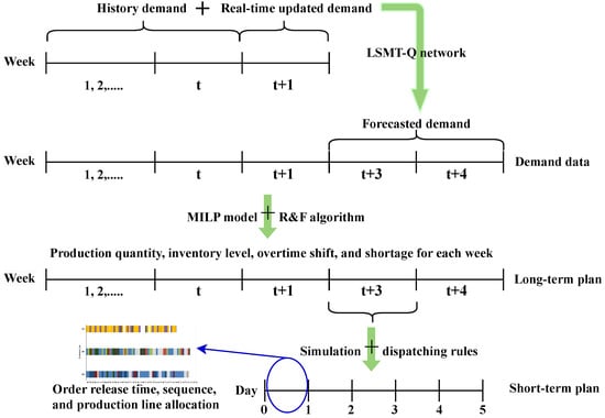
Figure 1.
The structure of data-driven methodology for HPP.
The data-driven methodology for HPP comprises three levels:
- The first level is data-driven demand forecasting. It uses an LSTM-Q network to iteratively update demand forecasts with historical and real-time demand data. The forecast period at this level is in weeks.
- The second level focuses on medium- and long-term planning. This level uses both known and predicted demand data to create plans for monthly and quarterly. The planning period at this level is in weeks. We generate production plans through a mixed-integer linear programming (MILP) model and employ the relax-and-fix algorithm to solve the MILP model.
- The third level is short-term planning. It refines the weekly production plans by specifying order release times and production sequences based on the results of the upper-level plans and supported by discrete-event simulation and dispatching rules.
4. Data-Driven Methodology for HPP
This section sequentially presents the three levels of the data-driven methodology for hierarchical production planning: demand forecasting, long-term planning, and short-term planning.
4.1. Demand Forecast
To forecast the requisite inventory levels for component parts over a forthcoming bi-weekly period, a novel hybrid neural network framework that integrated a Long Short-Term Memory (LSTM) network [33] and a Q-network, denoted as LSTM-Q network, is designed. The LSTM-Q is tailored to capture the temporal dependencies inherent in the historical data of part quantities spanning t consecutive weeks. Moreover, the LSTM-Q framework is designed to extract and integrate complex patterns and relationships from the time-series data, thereby facilitating a more robust and accurate prediction of part quantities necessary for the imminent two-week interval. The data information of continuous t weeks is represented as state vector , as shown in Equation (1).
In Equation (8), denotes the number of all parts in the tth week. Thus, we employ the LSTM to transform the variable-length state vector into a fixed-length vector .
As shown in Figure 2, the data information of all parts in is stored in the cell state . The cell state serves as a conveyor belt, transmitting pertinent information along the chain. Additionally, the cell generates a hidden state based on the current cell state. The forward propagation of the LSTM can be represented by Equations (2)–(6).
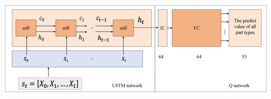
Figure 2.
LSTM-Q network structure.
In Equations (2)–(6), , , , and , , , represent the weight matrices and bias vector parameters. is the fully connected layer with activation function. is the forget gates. is the input gates. is the output gates.
The LSTM network can incorporate the data information of each week into the cell state. Therefore, the final hidden state captures all the data information belonging to the state , i.e., . The fixed-length vector is then connected to a deep Q network, which outputs the predicted number of all parts in next two weeks. The parameters of the LSTM-Q network used in this paper are shown in Table 2.
Table 2.
Parameters of LSTM-Q Networks.
4.2. Long-Term Planning
The primary goal of long-term planning is to generate a plan that specifies weekly product types, production quantities, overtime shift schedules, and inventory levels. We present a mathematical model constructed for long-term planning in Section 4.2.1, followed by a heuristic algorithm for solving the model in Section 4.2.2.
4.2.1. Mathematical Model
As described above, the fuel tank production workshop can be viewed as a flow shop, characterized by fast processing, high automation, and a simple production line layout. Each production line can process all product types, allowing the combined capacity of multiple lines to be treated as a single resource. We simplify the model by converting the production capacity of all production lines to the total production time in each planning period. The period duration is set longer than the maximum processing time for any individual product, meaning that, if production capacity allows, the entire product can be completed within one period. Overtime production is possible but capacitated, as the planner can reallocate workers and production lines from other workshops to address capacity shortages. However, reallocating workers and production lines from other workshops implies additional overtime costs, requiring a trade-off between overtime and shortage. In the mathematical model, we manage overtime by adding overtime shift constraints and assigning high overtime costs to avoid excessive overtime. In addition, the following basic assumptions underlie the long-term production planning scenarios.
- Assumptions:
- Each product is produced in a single production lot during a single production cycle.
- It should be noted that split batches of the same product in the same cycle are not considered.
- The relevant materials are sufficient in number and quality, and the production process is be disrupted by accidents.
- The production process is characterized by a 100% yield rate, indicating no wastage.
- The processing time represents the average total time per product, comprising not only the value-added processing time in machines but also other non-value-added activities, such as queuing and material handling.
- For the capacity constraints, production lines and workers are pre-configured, without consideration for splitting.
- The production capacity can be fully used, that is, the equipment is not in a state of disrepair or inoperable.
- The costs associated with inventory and shortage depend on the batch sizes of products.
- The setup costs are determined by whether a product type is scheduled for production in a specific period, regardless of the production quantity.
- The costs associated with overtime are only dependent on the shift schedules and number of shifts, not dependent on the specific product type or batch size.
- The model does not consider production costs, but rather the additional costs associated with inventory, setup, shortage, and overtime.
The parameters and symbols used to construct the mathematical model for the long-term production planning are defined as follows.
- Parameters and Symbols Definition:
| Symbol | Description |
| Index: | |
| i | Index representing product number, |
| t | Index representing the period number, |
| n | Index representing the overtime shift number, |
| Parameter: | |
| I | Total number of product categories. |
| T | Total number of planning periods. |
| N | Total number of overtime shifts during the unit period. |
| M | A big enough number. |
| Predicted demand for product i in period t. | |
| Unit inventory cost for product i. | |
| Unit shortage cost for product i. | |
| The setup cost for all product i in per period. | |
| R | Regular production capacity. |
| Overtime production capacity for period t and shift n in hours. | |
| Unit processing time for product i. | |
| Inventory capacity limit. | |
| The unit cost for overtime shift in period t. | |
| The set of positive integers. | |
| Integer variables: | |
| The production quantity of product i in period t. | |
| Inventory level for product i at period t. | |
| Actual shortage quantity for product i at period t. | |
| Binary variables: | |
| In period t, if the n th overtime shift is scheduled, the value of is 1; otherwise, the value of is 0. | |
| In period t, if the product i in period t is scheduled, the value of is 1; otherwise, the value of is 0. In other words, a setup operation occurs if a product is scheduled to be produced. | |
The problem we considered in long-term production planning belongs to multi-item capacitated lot-sizing problems with inventory constrains (MCLSP-I). The MCLSP-I can be formulated as a mixed integer linear programming model (denoted by ‘MILP model’):
- MILP Model:
Equation (7) represents the objective function of the mathematical model, comprising inventory costs, shortage costs, setup costs, and overtime costs. The objective is to minimize the total cost of the manufacturing system over the planning horizon. In this model, we focus more on inventory and shortage costs to streamline the mathematical formulation, thus ignoring production costs. Equation (8) represents the inventory balance constraints. At the end of each period, the quantity of the product remaining after fulfilling customer service demand is the inventory for that period. In the event of unfilled customer demand, the number of products not delivered on time is the shortage quantity. Equation (9) outlines the production capacity constraints. For any period, if there is no overtime, the total production work hours must not exceed the regular production capacity of the system. If overtime is engaged, the total production work hours cannot exceed the sum of the configured production capacity and overtime work hours. Equation (10) specifies the minimum production batch constraint, which states that for any product, the total production quantity over the planning horizon must be greater than or equal to the maximum expected demand across all periods. This prevents scenarios where a product has only a small demand in a certain horizon, potentially minimizing costs despite shortages, leading to ongoing out-of-stock status. Equation (11) guarantees that if no setup occurs during period t, the production quantity becomes zero. Equation (12) delineates the inventory capacity constraints, which limit the total warehouse inventory at the end of a period not to exceed the total warehouse capacity. Equation (13) defines the overtime shift constraints, indicating that the number of overtime shifts in a period must not exceed the upper limit of overtime production capacity. Equations (14)–(16) represent the fundamental constraints on the decision variables.
4.2.2. Relax-And-Fix Heuristic
The planning problem considered in this paper is a multi-item capacitated lot-sizing problem with inventory constraints, which is classified as strongly NP-hard [72]. The efficient resolution of such problems, particularly in large-scale scenarios, remains a significant challenge due to their computational complexity. To address this, we propose a relax-and-fix heuristic algorithm adapted to this class of problems. The methodology comprises three key steps: first, a pre-processing phase to generate a feasible solution rapidly; second, a comprehensive implementation of the R&F procedure; and third, the integration of heuristic cuts to accelerate the solution process further.
- (1)
- Pre-processing for finding feasible solutions
Providing the R&F algorithm with rapid and feasible solutions at an early phase can facilitate efficient guidance for the subsequent R&F approach. The binary variables are the key to solving mixed-integer programming models. Consequently, when seeking a feasible solution, our attention is directed towards the values of the binary variables and . The variable indicates whether product i is scheduled for production in period t. While scheduling all products for production in every period is suboptimal, it always results in a feasible solution. The physical meaning of is whether or not the nth shift in period t is scheduled for overtime. It is evident that if we do not consider overtime in the schedule even regular production shifts cannot cope with overtime, there are always feasible solutions. In such a scenario, customer demand that is not delivered on time would be transformed into a shortage. In other words, we let and ; in this case, the total overtime cost is zero, , while the setup cost is fixed at . The remaining decision variables can be obtained by solving the following integer linear programming model (denoted by ’ILP model’).
The objective Function (17) minimizes the total cost, which is the total inventory holding cost and shortage cost. Constraints (18) replace Constraints (9), with . Note that Constraints (13) and (15) in the MILP model are redundant for the ILP model due to ; therefore, they are removed in the ILP model. Compared to the MILP model, the ILP model is an integer linear programming model and can be solved faster. In the pre-processing stage, we use a commercial solverto obtain feasible solutions for the ILP model as the initial solution of the subsequent R&F algorithm to guide the algorithm.
- (2)
- Relax-and-fix approach
The R&F approach of this study is based on the works of Friske et al. in 2022 [48] and Wang et al. in 2023 [46]. The core idea of the R&F approach is to decompose the original problem into a series of subproblems, each solved iteratively. The decomposition focuses on binary variables and as the primary objects of optimization. Considering the studies mentioned above, this research employs a period-based decomposition method. We let K denote the total number of subproblems, corresponding to the number of iterations.
Each iteration comprises three blocks: the fixed block, the integer block, and the relaxed block. In each subproblem, the optimization targets the binary variables and in the integer block, which are maintained as 0–1 variables. The binary variables and in the fixed block are set to the values obtained from the previous iteration, while the remaining time intervals form the relaxed block, where binary variables and are relaxed to continuous variables in the range . The time interval of the integer block for each subproblem is defined as . If T is not an integer multiple of k, the length of the final subproblem interval is . The subproblems are solved using the CPLEX solver.
Figure 3 uses a small instance with to illustrate the fundamental logic of the iterative solution of the R&F method. As illustrated in Figure 3, this study employs a period-based decomposition method. The planning horizon is first divided into K time intervals. The integer block of each subproblem corresponds to one time interval, where the binary variables and within this interval are optimized. In the instance shown in Figure 3, with and , the time interval for each subproblem is three periods, while the last subproblem encompasses four periods. Once the decomposition is completed, an iterative solving process is performed. In the first iteration, since no results are available from prior iterations, this subproblem only comprises an integer block and a relaxed block, with no fixed block. In this iteration, and are treated as binary variables in the time interval , while and in the interval are treated as continuous variables. Solving this subproblem yields the solutions for and in the interval . In the second iteration, and in the interval are fixed to the solutions from the first iteration. and in the interval are treated as binary variables, while and in remain continuous. Solving the second subproblem provides solutions for and in . In the third and final iteration, and in the fixed block and are fixed to the solutions of the first and second iteration. The binary variables and in the interval of the integer block are then optimized, without the the relaxed block. After completing the third iteration, all binary variables are optimized and the final solutions are recorded. Pseudo-code Algorithm 1 provides a detailed explanation of the R&F algorithm logic.
| Algorithm 1 The procedure of the R&F method. |
|
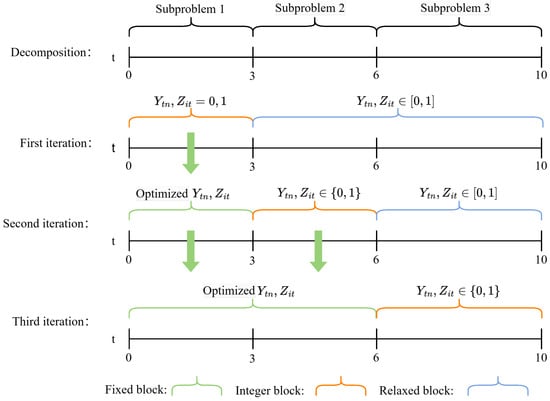
Figure 3.
An example of the basic iterative logic in the R&F approach.
- (3)
- Method for accelerating computations
To accelerate the computation, we tight the constraints (11) in this LP-relaxation by defining M as follows:
To enhance the computational efficiency of the R&F algorithm, we extend the relaxation of variables. In the relaxed block of the subproblem, we not only allow binary variables to take on continuous values between 0 and 1 but also relax the integer variable to a continuous variable. Throughout the iterative process, is progressively constrained back to integer values. Since both inventory and shortages are calculated from , we can also relax and to continuous variables. As becomes bounded to integer values during the iterations, and are automatically converted to integers as well. This approach effectively accelerates the solution of the subproblem. We define the R&F algorithm in Pseudo-code Algorithm 1 without the acceleration method as R&F-1, and the R&F with the acceleration method as R&F-2.
4.3. Short-Term Planning Based on Simulation and Dispatching Rules
The main task of short-term planning is to refine production planning by batching orders and determining their release time and sequence. This process is guided by the planned products, quantities, and overtime shifts established in the long-term production planning. Unlike long-term planning, which treats all production lines as a single resource, short-term planning must consider more detailed constraints.
Specifically, the fuel tank workshop contains several production lines, requiring equipment setup changes when switching between different products. Thus, the plan should avoid frequent line changeovers. In addition, material transfer between machines on a production line is based on trolleys. This means that we need to consider the resource constraints of trolleys in short-term planning. To optimize resource utilization, production batch sizes should avoid being too small and ideally match multiples of the trolley capacity.
This study introduces an approach based on simulation and dispatching rules for short-term planning. First, orders are scheduled based on dispatching rules. Second, they are simulated to verify the operational feasibility of short-term plans through key performance indicators (KPIs) such as order completion times. The simulation results can provide decision support for plan adjustments. Furthermore, the simulation validation experiment is conducted only at the beginning of each week. If an emergency order arrives during the week, only the short-term plan is updated according to the dispatching rules. Based on existing dispatching rules, we propose two new dispatching rules that incorporate the earliest due date (EDD) rule and develop a hybrid dispatching strategy based on these two rules. The core ideas and main steps of these three approaches are outlined below.
4.3.1. Dispatching Rules Based on Time-Window
The dispatching rules based on time-window balance on-time delivery and production efficiency by aggregating orders of the same type with similar due dates. The core mechanism groups orders into batches according to predefined time windows and adjusts batch sizes through splitting/merging orders to meet production line constraints, e.g., trolley capacity and changeover number. While prioritizing on-time delivery, the approach requires balancing time window granularity with economies of scale. If the time window is too large, this method may create oversized batches leading to excessive WIP inventory, whereas overly small windows increase changeover frequency. The key steps of this rule are as follows:
- (1)
- Order encoding and initial sorting: Map due date to time-window identifiers, convert part numbers into product codes, and sort orders in ascending order of due dates to generate an initial order queue.
- (2)
- Dynamic batching based on time window: Perform batching sequentially in each time window. First, combine orders for the same product in the same time window. Then, evaluate batch sizes: split oversized batches into smaller ones based on trolley capacity and defer undersized batches to the next time domain for further combination.
- (3)
- Resource allocation: Recalculate the due date for each batch, which is determined by the latest due date among its constituent orders. Allocate decoded orders to available production lines using the EDD rule, prioritizing lines with no changeovers.
The key parameter of this method is the length of the time window. Adjusting the time-window length optimizes the balance between batch economics and resource constraints. For short-term planning with a weekly planning horizon, we consider four rule variants with time-window lengths of 4, 6, 8, and 12 h, labeled as TW-4, TW-6, TW-8, and TW-12, respectively.
4.3.2. Dispatching Rules Based on Available Capacity
The dispatch rule based on the available capacity minimizes the changeover of production lines by aggregating orders of the same type based on a fixed capacity threshold. The core mechanism groups orders by product type and forms production batches constrained by a preset capacity threshold (e.g., 2-h production capacity). This approach reduces the number of changeovers by centralizing production and relying on finished product inventories to buffer due date variances.
- (1)
- Order encoding and initial sorting: Extract the product type and due date of orders, convert them into product codes, and sort orders in ascending order of due dates to generate an initial order queue.
- (2)
- Dynamic batching based on available capacity: Traverse the orders cyclically, dynamically fill the batch with the capacity threshold for each product type. When the capacity threshold is exceeded, generate a new batch.
- (3)
- Resource allocation: This step is the same as Step 3 of dispatching rules based on time-window.
The key parameter of this method is the size of the capacity threshold, which can be adjusted to optimize the balance between batch economics and resource constraints. The short-term schedule is based on a weekly planning cycle, and since the regular working time of each production line is 8 h per day, we consider four rule variants with capacity threshold sizes of 2/4/6/8 h, which are defined as AC-2, AC-4, AC-6, AC-8.
4.3.3. Hybrid Dispatching Strategy
The hybrid strategy integrates two dispatching rules: those based on the time window and based on the available capacity, with a particular focus on trolley resource constraints. In the workshop, limited trolley resources represent a bottleneck. So this strategy prioritizes the production of products that consume more bottleneck resources, specifically products with smaller single-trolley capacities.
- (1)
- Order encoding and initial sorting: This step is the same as Step 1 of dispatching rules based on available capacity.
- (2)
- Dynamic batching based on the hybrid strategy: First, divide the order queue by the time window. In each time window, aggregate half products with smaller single-trolley capacities. For the remaining half products, dynamically fill batches based on the threshold of available capacity ignoring the time window.
- (3)
- Resource allocation: This step is the same as Step 3 of dispatching rules based on time-window.
The hybrid strategy requires parametrization of both two dispatching rules. In the implementation, we first test which variants of the two basic rules perform optimally and then apply the settings from these variants in the hybrid strategy.
5. Experiments and Results
This section comprises four main components. First, Section 5.1, Section 5.2 and Section 5.3 respectively present the performance test results for the three levels of the HPP system. Finally, Section 5.4 discusses the overall performance of the system as a whole.
The experiments in this section are run on a personal computer equipped with an Intel Core i5-10310U CPU 1.70 GHz/2.21 GHz and 16 GB of RAM. The proposed methods are implemented with Python 3.9.4, CPLEX Studio 22.1.0, and Anylogic 8.5. CPLEX Studio 22.1.0 is used for algorithm implementation and verification in Section 5.2, and Anylogic 8.5 is used for simulation in Section 5.3.
5.1. Results of Demand Forecast
5.1.1. Training Process
During training, datasets are production data obtained from a company. The training process employs the parameters outlined in Table 3. Figure 4 shows the loss values for each training epoch on the dataset.
Table 3.
The training parameters of LSTM-Q network.
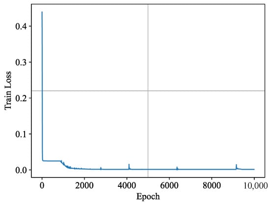
Figure 4.
Loss curve of the LSTM-Q.
Figure 4 illustrates a gradual decrease in the loss value throughout the training process, indicating that the proposed LSTM-Q network framework achieves high-quality predict performance.
5.1.2. Validation of the Proposed LSTM-Q Network Framework
To verify the efficacy of the LSTM-Q network, a predictive analysis was conducted utilizing an actual production dataset to forecast the order quantities for 53 different parts over the upcoming two-week period. The comparison between the forecasted quantities and the actual order quantities is illustrated in Figure 5. As depicted, the trend lines for the predicted order quantities and the actual order quantities of the 53 parts exhibit a high degree of alignment (with the forecasted values closely mirroring the actual values), thereby demonstrating the LSTM-Q network’s proficient predictive performance.
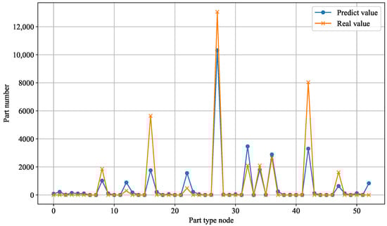
Figure 5.
The real and predicted demand numbers of all part types in the next two weeks.
5.1.3. Computational Experiments and Analysis
In the realm of predictive analytics, the performance of neural networks is often benchmarked by the proximity of their forecasted outputs to actual data. For LSTM-Q, Gated Recurrent Unit (GRU) networks, and Recurrent Neural Networks (RNNs), this proximity is quantifiably measured by the ‘gap’ value—the difference between predicted order quantities and actual order quantities. A smaller gap value signifies superior predictive performance of the network. Table 4 below summarizes the mean and standard deviation of the gap values for both LSTM and GRU networks, where each network was run 20 times on each test case to ensure robust statistical assessment. The mean gap value (mean) represents the average difference over the multiple runs, offering insight into the overall forecasting accuracy of the networks. Meanwhile, the standard deviation (std) provides a measure of the variability in the predictive performance across the runs, with a smaller standard deviation indicating more consistent performance.
Table 4.
Comparison results of LSTM-Q, GRU, and RNN networks (mean/std).
The proposed LSTM-Q network exhibits remarkable predictive performance compared to existing methodologies. Table 4 reports the comparison results, and the ones marked in bold in this table are the optimal results. As presented in Table 4, the LSTM-Q network achieves an impressive average prediction accuracy of 98.9%, surpassing the RNN with 93.8% accuracy and GRU with 98.5%. Specifically, RNNs employed for forecasting France’s day-ahead and year-ahead load demand have demonstrated prediction accuracies ranging from 98.51% to 98.92% [73]. Additionally, Honjo et al. [74] developed a Gated Recurrent Unit (GRU) network model that achieved a prediction accuracy of 96%, representing a 15% increase over conventional forecasting methods.
Comparative analysis reveals that the LSTM-Q network consistently maintains a smaller mean prediction gap across the majority of forecasting instances, indicating its superior ability to capture intricate temporal dependencies and non-linear demand patterns inherent in order data. While the prediction stability of the LSTM-Q, GRU, and RNN models shows negligible differences, all three models demonstrate commendable robustness. Nevertheless, the LSTM-Q network’s higher average accuracy underscores its effectiveness in delivering more precise and reliable demand forecasts.
To evaluate the computational efficiency of the proposed algorithms, we measured the prediction times of LSTM-Q, GRU, and RNN across different week intervals ranging from 1–2 weeks to 8–9 weeks. As illustrated in Table 5 (the best results are in bold), all three models exhibit minimal time costs, with GRU and RNN generally outperforming LSTM-Q in terms of speed. This low computational burden ensures that the models are highly suitable for real-time scenarios, enabling swift and accurate predictions without significant delays.
Table 5.
Time cost comparison of neural networks (seconds).
5.2. Results of Long-Term Planning
This section evaluates the performance of the proposed R&F algorithms in solving long-term planning models. The experiments comprises two parts. First, we randomly generate some instances of different sizes to test the performance of the proposed R&F algorithms. We also perform a sensitivity analysis to examine how the number of sub-problems affects solution quality and solving speed. Second, the proposed R&F algorithm is applied to a real-world case in a fuel tank manufacturing factory.
5.2.1. Experiments with Randomly Generated Instances
- (1)
- Instance Generation
Table 6 presents the key parameters for generating the instance dataset. The primary parameters include the number of products, the planning horizon, demand, process time, and initial inventory. We define three different values for the number of products to represent three problem scales, including small, medium, and large. Demand quantity, process time, and initial inventory are generated randomly using a uniform distribution (denoted by U in Table 6). We classify demand into high demand (HD) and low demand (LD), and process time into long process time (LP) and short process time (SP). Using a full factorial design, we generated 10 instances for each combination of these five parameters, resulting in a total of 240 instances (2 × 3 × 2 × 2 × 1 × 10).
Table 6.
Parameters for randomly generated instances.
In addition to the key parameters, other parameters are set based on the real case, while cost-related parameters are primarily referenced from existing literature [46,75]. The setup costs are generated as follows:
where represents the average demand of product i, and is the time between orders (TBO).
- (2)
- Performance Analysis
The performance evaluation experiments aim to validate the effectiveness of the proposed algorithms and compare the performance of the two R&F variants. We benchmark the proposed algorithms against CPLEX, with a time limit of 2 h for CPLEX and 10 min for the R&F algorithms. The number of subproblems K is set to three based on the findings in existing studies [46,76].
Table 7 summarizes the experimental results, where LD and HD represent demand ranges of U [100, 2000] and U [2000, 4000], respectively, while SP and LP correspond to processing time ranges of U [36, 72] and U [72, 120], respectively. Performance metrics include the optimal objective value (denoted as Obj), which is the best value found within the time limit, computation time (CT), and the average gap (denoted as Ave.Gap) and maximum gap (denoted as Max.Gap) relative to CPLEX. The gap is calculated as follows:
where and are the objective values obtained by solving the MILP model with CPLEX directly and by using the R&F methods, respectively.
Table 7.
The experiment results with comparisons for the problem instances randomly generated.
The experimental results in Table 7 are analyzed under two scenarios, and the best results are marked in bold. In the first scenario, CPLEX can find the optimal solution within the time limit (i.e., for CPLEX). In this case, the gap of the R&F algorithms measures their deviation from the optimal solution, with smaller gaps indicating better performance. Both proposed R&F algorithms achieve an average gap of less than 1% and a maximum gap below 2%, outperforming CPLEX in computation time. Notably, the R&F-2 algorithm demonstrates higher stability, with an average gap below 0.8% and a maximum gap under 1%.
In the second scenario, CPLEX fails to find the optimal solution within the time limit (i.e., for CPLEX) and returns only feasible solutions. In this case, a positive gap indicates that the R&F algorithms obtain better solutions than CPLEX, corresponding to lower-cost production plans. Experimental results show that both R&F-1 and R&F-2 algorithms consistently outperform CPLEX in solution quality and computation time. While R&F-1 occasionally produces slightly better solutions than R&F-2, the difference is marginal. However, R&F-2 significantly outperforms R&F-1 in computation speed.
In summary, both proposed R&F algorithms efficiently solve the MILP model, generating high-quality long-term production plans. R&F-2 exhibits superior performance in terms of computation speed and stability compared to R&F-1.
- (3)
- Sensitivity analysis
The existing literature demonstrates that the number of subproblems K significantly impacts both solution quality and computational efficiency in R&F algorithms [76]. Therefore, we conduct a sensitivity analysis on the number of subproblems K for the R&F-2 algorithm, which was shown to be the best-performing variant in Section 5.2.1. For the 240 instances in the test dataset, we vary K from 2 to 10 with a step size of 1, running each instance 9 times with different K values. Note that corresponds to solving the original problem directly using CPLEX without decomposition. The analysis is performed across three instance scales: small (), medium (), and large ().
Figure 5 and Figure 6 compare the performance of the R&F-2 algorithm under different K values for various problem scales. Performance is evaluated using two metrics: (1) the average value of objective gap computed by Equation (21) and (2) the average value of computation time gap , calculated as
where and are the computation time spent to solve the MILP model with CPLEX directly and by using the R&F-2 method, respectively.
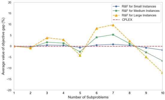
Figure 6.
Comparison of the average of the R&F-2 algorithm with different K.
A positive indicates that R&F-2 is faster than CPLEX, with larger values representing better performance. For small-scale instances, a smaller indicates that the R&F-2 solution is closer to optimal. Figure 6 and Figure 7 show that R&F-2 achieves the best balance between solution quality and computation speed at . For medium- and large-scale instances, where CPLEX sometimes fails to find optimal solutions within the time limit, a larger average indicates better performance. In these cases, R&F-2 performs optimally at . Additionally, Figure 7 reveals that the computation time of the R&F-2 algorithm increases with the number of subproblems K, suggesting that excessive decomposition should be avoided. The optimal K value depends on the problem scale and should be determined based on specific instance characteristics.
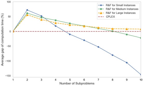
Figure 7.
Comparison of the average of the R&F-2 algorithm with different K.
5.2.2. Experiments with Real-World Instances
This case study implements the R&F-2 algorithm in a real-world fuel tank manufacturing plant. The production system comprises three parallel lines producing 53 different products. The production capacity of these lines is represented by the total available hours, which accounts for the plant’s limited capacity. Table 8 details the parameter configuration in our mathematical model where cost-related parameters are adjusted based on experimental tuning to meet the real planning requirements.
Table 8.
Parameter configuration.
We evaluate the performance of the R&F-2 algorithm under different planning horizons, including monthly (T = 4), two-month (T = 8), quarterly (T = 12), and annual (T = 52) plans. Each period corresponds to one week in the production planning. First, we compare the R&F-2 algorithm with the Genetic algorithm (GA) implemented in the original system. The original system employs GA with two selection strategies: roulette wheel selection (defined as GA_R) and tournament selection (defined as GA_T). The parameters for the genetic algorithm are set as follows: Population size is 100, mutation probability is 0.1, and crossover probability is 0.8. For different planning horizons (T = 4, 8, 12, 52), the maximum generations are set to [1500, 3000, 3000, 10,000], respectively. We compare the R&F-2 algorithm with the two GAs based on two metrics, including computational time (CT) and the comparison coefficient (CC) with R&F-2, calculated as the ratio of the optimal results obtained by the GAs to those obtained by the R&F-2 algorithm. Table 9 reports the comparison results. The higher values of the comparison coefficient for GAs indicate superior solution quality of R&F-2. The experimental results in Table 9 indicate that R&F-2 outperforms GAs in both solution quality and speed, particularly when handling large-scale problems, such as quarterly and annual planning horizons.
Table 9.
Comparison results.
Second, we carefuly evaluate the performance of R&F-2 in Table 10. Our implementation optimizes the total cost while monitoring five key performance indicators (KPIs):
Table 10.
Implementation results of R&F-2 algorithm for different planning horizons.
- (1)
- The computation time measures the efficiency of the algorithm execution. Notably, when implementing the R&F-2 algorithm, the time limit is set to 600 s based on the planning requirements of the real factory.
- (2)
- The average inventory level allows planners to evaluate the inventory status, guiding the setup of safety stock and efficient management of storage space, calculated as
- (3)
- The average utilization of production capacity measures the ratio of planned production capacity to the total available capacity, helping to assess whether the production system is appropriately loaded. is calculated as
- (4)
- The average utilization of overtime shifts reflects the proportion of overtime shifts scheduled relative to the total number of shifts available. This metric assists planners in optimizing overtime schedules and determining whether additional production lines and workers are necessary to enhance factory capacity from a long-term perspective. is calculated as follows:
- (5)
- The average rate of on-time delivery indicates the proportion of orders delivered on time to the total number of orders during the whole planning horizon, and it is an important indicator to measure the service level. is calculated as follows:where presents the number of on-time delivery orders during period t.
Table 10 demonstrates that the R&F-2 algorithm efficiently generates optimized production plans for both medium-term (1 to 2 months) and long-term (quarterly, semi-annual, and annual) horizons. The computation speed is impressive, especially for production planning of less than six months. In contrast, CPLEX is already very difficult to handle for a two-month program, and the suboptimal feasible solutions obtained within the two-hour time limit are worse than solutions obtained by the R&F-2 algorithm.
The experimental results reveal the average rate of on-time delivery below 100%, mainly due to inventory capacity constraints. During demand fluctuation peaks, even with sufficient production capacity, inventory space limitations prevent 100% fulfillment of customer demands. Nevertheless, the achieved service level exceeds 99%, surpassing the target threshold of 95%.
Table 4 reports that the average utilization of overtime shifts mostly exceeds 50%, and the average utilization of production capacity is above 90%. These metrics indicate inherent production capacity limitations in the current workshop configuration. Although the current workshop can handle the existing demand for products, it relies heavily on overtime shifts and support from other workshops. This indicates that the system lacks resilience to accommodate sudden demand surges or new products. From a long-term perspective, it is necessary to consider expanding production lines and workers or exploring task redistribution to other workshops to avoid additional costs due to transfer and overtime shifts.
5.3. Results of Short-Term Planning
The experiments for short-term planning use data derived from the long-term production plan of the fuel tank workshop. Specifically, the dataset consists of actual orders for a specific week, matching the planned production quantities and product types. The order data contains 2506 orders for 11 product types. The workshop comprises three parallel production lines, and products are transferred between machines on the production lines using specific trolley resources. Different product types require different types of trolleys with varying capacities. Table 11 presents detailed information about the products and their corresponding trolley types.
Table 11.
Product types and their corresponding trolley capacities.
We develop a simulation model for the fuel tank workshop, as illustrated in Figure 8, and perform simulation experiments to analyze the dispatching rules. The key evaluation metrics include the average utilization of equipments, the number of changeovers, and average inventory levels. Figure 9 reports the results of these experiments.
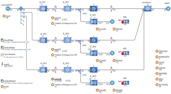
Figure 8.
Simulation model of short-term planning for a fuel tank manufacturing workshop.
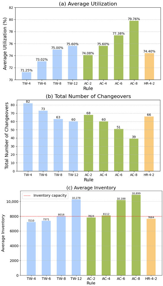
Figure 9.
Simulation results of short-term planning for different dispatching rules.
We first implement the variants of two basic dispatching rules, including TW-4, TW-6, TW-8, and TW-12 for rules based on time window, and AC-2, AC-4, AC-6, and AC-8 for rules based on available capacity. The results in Figure 9 demonstrate that the dispatching rules based on the time window effectively reduce the average inventory level, with the lowest inventory achieved when the time window is set to 4 h. On the other hand, the dispatching rules based on the available capacity significantly reduce the number of changeovers, with the fewest changeovers observed when the capacity threshold is set to 8 h. However, this setting results in a higher average inventory level compared to the inventory capacity of 8000.
Based on the experimental results of basic dispatching rules, we employ a hybrid dispatching strategy with the time window of 4 h and the capacity threshold of 2 h, denoted as HR-4-2. Figure 9 also presents the experimental results for this hybrid strategy. The experiments demonstrate that the hybrid strategy yields optimal results by reducing the number of changeovers while maintaining a low inventory level.
In addition, we compare the hybrid dispatching strategy HR-4-2 with the original system’s dispatching approach. In the original system, the short-term planning is generated by planners based on EDD rules and their practical field experience. Table 12 presents the results before and after optimization. The comparison demonstrates the effectiveness of the proposed method HR-4-2, which maintains the average inventory below the inventory capacity, significantly reduces the number of changeovers, and enhances resource utilization.
Table 12.
Comparison before and after optimization.
5.4. Discussion of System Efficiency
Because the HPP is a whole system, we provide a discussion on the overall operational efficiency of the HPP. Table 13 presents the average time required for updating the demand forecast, long-term plan, and short-term plan components of the proposed HPP system. In the demand forecasting layer, the forecasting process is rapid enough to allow for updates as soon as a new order arrives. This timely adjustment can enhance the iterative learning of the LSTM-Q algorithm. However, to prevent data redundancy, enterprises may choose to establish an update cycle based on actual requirements. In the long-term planning level, we detail the time spent updating the monthly, quarterly, and annual plans. The quarterly and annual plans do not require frequent updates; therefore, the monthly plan is typically revised in response to changes in demand, with updates occurring weekly. Consequently, the average time for a single execution of the entire HPP system is approximately 32.999 s.
Table 13.
Efficiency analysis of HPP system.
Furthermore, the validation of the simulation primarily focuses on the short-term plan. The simulation validation experiment is conducted only at the beginning of each week, coinciding with the development of the short-term plan for the week. If demand or system conditions change during the week, only the short-term plan is updated according to the dispatching rules. Thus, without running the simulation, the processing time for the HPP system is approximately 0.770 s. It indicates that the updates for the demand forecast, long-term plan, and short-term plan can be completed in under one second.
6. Conclusions and Perspective
This paper proposes a data-driven methodology for hierarchical production planning specific to fuel tank workshops. First, we propose an LSTM-Q network for demand forecast. Experimental results demonstrate that the LSTM-Q network can effectively forecast demand in the real-world case and outperform the gated recurrent unit network. Second, we develop two R&F algorithms to solve the MCLSP-I for long-term planning based on the demand data obtained from the first level. Both R&F algorithms can efficiently generate high-quality production planning, and the R&F-2 algorithm exhibits better performance in computation speed and stability compared to the R&F-1 algorithm. Third, short-term planning uses long-term plans as input and applies simulation and dispatching rules to generate plans. The experiments compare the three proposed dispatching rules. The results indicate that the hybrid dispatching rule is optimal for the fuel tank workshop and can effectively balance the inventory level and changeover frequency.
Based on the limitations of this study, future research directions can focus on the following three points. The first direction is to enhance the demand forecast towards stochastic scenario trees. The proposed approach to demand prediction generates only a single quantity of demand for a single product and period. However, this approach can not handle more complex demand fluctuations. Future research could explore generating demand forecasts in the form of scenario trees to support stochastic programming for production planning. The second direction is to extend the deterministic mathematical model of MCLSP-I to a stochastic programming model that can generate production plans to accommodate various demand scenarios. The third direction is to enrich the dispatching rules. This paper evaluates limited dispatching rules. Future research could build a comprehensive dispatching rule library and use deep reinforcement learning to support real-time dynamic decision-making.
Author Contributions
D.L.: Writing—original draft, Methodology, Data curation. L.D.: Visualization, Investigation, Formal analysis, Writing—review and editing. Z.G.: Supervision, Project administration, Conceptualization. W.F.: Visualization, Project administration. H.Z.: Writing—review and editing, Visualization, Project administration. All authors have read and agreed to the published version of the manuscript.
Funding
This work was supported by the National Key Research and Development Program of China under Grant No. 2023YFB3307900.
Data Availability Statement
The data are available at https://doi.org/10.5281/zenodo.14956370 (accessed on 27 February 2025).
Conflicts of Interest
The authors declare no conflicts of interest.
References
- Mota, A.L.S.; Lins, R.G. Production of customized commercial vehicles in assembly line based on modified-to-order demands: A novel method and study case. Int. J. Prod. Econ. 2025, 282, 109535. [Google Scholar] [CrossRef]
- Sahebjamnia, N.; Torabi, S.A.; Mansouri, S.A. Building organizational resilience in the face of multiple disruptions. Int. J. Prod. Econ. 2018, 197, 63–83. [Google Scholar] [CrossRef]
- Pi, Z.; Wang, K.; Wei, Y.M.; Huang, Z. Transitioning from gasoline to electric vehicles: Electrification decision of automakers under purchase and station subsidies. Transp. Res. Part Logist. Transp. Rev. 2024, 188, 103640. [Google Scholar] [CrossRef]
- Ghazali, A.K.; Aziz, N.A.A.; Hassan, M.K. Advanced algorithms in battery management systems for electric vehicles: A comprehensive review. Symmetry 2025, 17, 321. [Google Scholar] [CrossRef]
- Bakhshi-Khaniki, H.; Fatemi Ghomi, S. Integrated dynamic cellular manufacturing systems and hierarchical production planning with worker assignment and stochastic demand. Int. J. Eng. 2023, 36, 348–359. [Google Scholar] [CrossRef]
- McKay, K.N.; Safayeni, F.R.; Buzacott, J.A. A review of hierarchical production planning and its applicability for modern manufacturing. Prod. Plan. Control 1995, 6, 384–394. [Google Scholar] [CrossRef]
- O’Reilly, S.; Kumar, A.; Adam, F. The role of hierarchical production planning in food manufacturing SMEs. Int. J. Oper. Prod. Manag. 2015, 35, 1362–1385. [Google Scholar] [CrossRef]
- Iwamura, K.; Morinaga, E.; Hirahara, Y.; Fukuda, M.; Niinuma, A.; Oshima, H.; Namioka, Y. A study on hierarchical production planning framework for engineer-to-order production of large products. In Proceedings of the International Symposium on Flexible Automation, Seattle, WA, USA, 21–24 July 2024; American Society of Mechanical Engineers: New York, NY, USA, 2024; Volume 87882, p. V001T06A002. [Google Scholar]
- Soori, M.; Arezoo, B.; Dastres, R. Virtual manufacturing in industry 4.0: A review. Data Sci. Manag. 2024, 7, 47–63. [Google Scholar] [CrossRef]
- Qi, Q.; Tao, F. Digital twin and big data towards smart manufacturing and industry 4.0: 360 degree comparison. IEEE Access 2018, 6, 3585–3593. [Google Scholar] [CrossRef]
- Luo, D.; Thevenin, S.; Dolgui, A. A state-of-the-art on production planning in Industry 4.0. Int. J. Prod. Res. 2023, 61, 6602–6632. [Google Scholar] [CrossRef]
- Zeng, X.; Yi, J. Analysis of the impact of big data and artificial intelligence technology on supply chain management. Symmetry 2023, 15, 1801. [Google Scholar] [CrossRef]
- Karkaria, V.; Tsai, Y.K.; Chen, Y.P.; Chen, W. An optimization-centric review on integrating artificial intelligence and digital twin technologies in manufacturing. Eng. Optim. 2024, 57, 161–207. [Google Scholar] [CrossRef]
- Mehra, A.; Minis, I.; Proth, J. Hierarchical production planning for complex manufacturing systems. Adv. Eng. Softw. 1996, 26, 209–218. [Google Scholar] [CrossRef]
- He, N.; Zhang, D.; Li, Q. Agent-based hierarchical production planning and scheduling in make-to-order manufacturing system. Int. J. Prod. Econ. 2014, 149, 117–130. [Google Scholar] [CrossRef]
- Boujnah, I.; Tlili, M.; Korbaa, O. Hierarchical production planning frameworks for multi product multi stage batch plants. In Proceedings of the 2023 International Conference on Innovations in Intelligent Systems and Applications (INISTA), Hammamet, Tunisia, 20–23 September 2023; IEEE: New York, NY, USA, 2023; pp. 1–6. [Google Scholar]
- Gfrerer, H.; Zäpfel, G. Hierarchical model for production planning in the case of uncertain demand. Eur. J. Oper. Res. 1995, 86, 142–161. [Google Scholar] [CrossRef]
- Meybodi, M.Z.; Foote, B.L. Hierarchical production planning and scheduling with random demand and production failure. Ann. Oper. Res. 1995, 59, 259–280. [Google Scholar] [CrossRef]
- Yan, H.S. Hierarchical stochastic production planning for flexible automation workshops. Comput. Ind. Eng. 2000, 38, 435–455. [Google Scholar] [CrossRef]
- Okuda, K. Hierarchical structure in manufacturing systems: A literature survey. Int. J. Manuf. Technol. Manag. 2001, 3, 210–224. [Google Scholar] [CrossRef]
- Thomas, D.J.; Griffin, P.M. Coordinated supply chain management. Eur. J. Oper. Res. 1996, 94, 1–15. [Google Scholar] [CrossRef]
- Kusumawati, R. Integrating big data analytics into supply chain management: Overcoming data silos to improve real-time decision-making. Int. J. Adv. Comput. Methodol. Emerg. Technol. 2025, 15, 17–26. [Google Scholar]
- Ge, D.; Pan, Y.; Shen, Z.J.; Wu, D.; Yuan, R.; Zhang, C. Retail supply chain management: A review of theories and practices. J. Data Inf. Manag. 2019, 1, 45–64. [Google Scholar] [CrossRef]
- Tao, F.; Zhang, H.; Liu, A.; Nee, A.Y. Digital twin in industry: State-of-the-art. IEEE Trans. Ind. Inform. 2018, 15, 2405–2415. [Google Scholar] [CrossRef]
- Chabanet, S.; Bril El-Haouzi, H.; Morin, M.; Gaudreault, J.; Thomas, P. Toward digital twins for sawmill production planning and control: Benefits, opportunities, and challenges. Int. J. Prod. Res. 2023, 61, 2190–2213. [Google Scholar] [CrossRef]
- Lanzini, M.; Adami, N.; Benini, S.; Ferretti, I.; Schieppati, G.; Spoto, C.; Zanoni, S. Implementation and integration of a Digital Twin for production planning in manufacturing. In Proceedings of the 35th European Modeling & Simulation Symposium, EMSS, Athens, Greece, 18–23 September 2023; CALTEK srl.: Busto Arsizio, Italy, 2023. [Google Scholar] [CrossRef]
- van de Berg, D.; Shah, N.; del Rio-Chanona, E.A. Hierarchical planning-scheduling-control—Optimality surrogates and derivative-free optimization. Comput. Chem. Eng. 2024, 188, 108726. [Google Scholar] [CrossRef]
- Meybodi, M.Z. Integrating production activity control into a hierarchicalproduction-planning model. Int. J. Oper. Prod. Manag. 1995, 15, 4–25. [Google Scholar] [CrossRef]
- Anderson, E.G., Jr.; Joglekar, N.R. A hierarchical product development planning framework. Prod. Oper. Manag. 2005, 14, 344–361. [Google Scholar] [CrossRef]
- De Kok, A. Hierarchical production planning for consumer goods. Eur. J. Oper. Res. 1990, 45, 55–69. [Google Scholar] [CrossRef]
- Neureuther, B.D.; Polak, G.G.; Sanders, N.R. A hierarchical production plan for a make-to-order steel fabrication plant. Prod. Plan. Control 2004, 15, 324–335. [Google Scholar] [CrossRef]
- Dcoutho, J.F.; Eisenbart, B.; Kulkarni, A. Hierarchy priortization and dynamic simulation for low volume production planning. In Proceedings of the 2023 IEEE Engineering Informatics, Melbourne, Australia, 9–13 September 2023; IEEE: New York, NY, USA, 2023; pp. 1–10. [Google Scholar]
- Hochreiter, S.; Schmidhuber, J. Long short-term memory. Neural Comput. 1997, 9, 1735–1780. [Google Scholar] [CrossRef]
- Gers, F.A.; Schmidhuber, J.; Cummins, F. Learning to forget: Continual prediction with LSTM. Neural Comput. 2000, 12, 2451–2471. [Google Scholar] [CrossRef]
- Sundermeyer, M.; Schlüter, R.; Ney, H. Lstm neural networks for language modeling. In Proceedings of the Interspeech, Portland, OR, USA, 9–13 September 2012; Volume 2012, pp. 194–197. [Google Scholar]
- Greff, K.; Srivastava, R.K.; Koutník, J.; Steunebrink, B.R.; Schmidhuber, J. LSTM: A search space odyssey. IEEE Trans. Neural Netw. Learn. Syst. 2016, 28, 2222–2232. [Google Scholar] [CrossRef] [PubMed]
- Siami-Namini, S.; Tavakoli, N.; Namin, A.S. A comparison of ARIMA and LSTM in forecasting time series. In Proceedings of the 2018 17th IEEE International Conference on Machine Learning and Applications (ICMLA), Orlando, FL, USA, 17–20 December 2018; IEEE: New York, NY, USA, 2018; pp. 1394–1401. [Google Scholar]
- Karimi, B.; Ghomi, S.F.; Wilson, J. The capacitated lot sizing problem: A review of models and algorithms. Omega 2003, 31, 365–378. [Google Scholar] [CrossRef]
- Helber, S.; Sahling, F. A fix-and-optimize approach for the multi-level capacitated lot sizing problem. Int. J. Prod. Econ. 2010, 123, 247–256. [Google Scholar] [CrossRef]
- Stadtler, H.; Sahling, F. A lot-sizing and scheduling model for multi-stage flow lines with zero lead times. Eur. J. Oper. Res. 2013, 225, 404–419. [Google Scholar] [CrossRef]
- Toledo, C.F.M.; da Silva Arantes, M.; Hossomi, M.Y.B.; França, P.M.; Akartunalı, K. A relax-and-fix with fix-and-optimize heuristic applied to multi-level lot-sizing problems. J. Heuristics 2015, 21, 687–717. [Google Scholar] [CrossRef]
- Pochet, Y.; Wolsey, L.A. Production Planning by Mixed Integer Programming; Springer: Berlin/Heidelberg, Germany, 2006; Volume 149. [Google Scholar]
- Araujo, K.A.G.d.; Birgin, E.G.; Kawamura, M.; Ronconi, D.P. Relax-and-fix heuristics applied to a real-world lot sizing and scheduling problem in the personal care consumer goods industry. Oper. Res. Forum 2023, 4, 47. [Google Scholar] [CrossRef]
- Joncour, C.; Kritter, J.; Michel, S.; Schepler, X. Generalized relax-and-fix heuristic. Comput. Oper. Res. 2023, 149, 106038. [Google Scholar] [CrossRef]
- Clark, A.R.; Clark, S.J. Rolling-horizon lot-sizing when set-up times are sequence-dependent. Int. J. Prod. Res. 2000, 38, 2287–2307. [Google Scholar] [CrossRef]
- Wang, S.; Zhang, H.; Chu, F.; Yu, L. A relax-and-fix method for clothes inventory balancing scheduling problem. Int. J. Prod. Res. 2023, 61, 7085–7104. [Google Scholar] [CrossRef]
- Brahimi, N.; Aouam, T. Multi-item production routing problem with backordering: A MILP approach. Int. J. Prod. Res. 2016, 54, 1076–1093. [Google Scholar] [CrossRef]
- Friske, M.W.; Buriol, L.S.; Camponogara, E. A relax-and-fix and fix-and-optimize algorithm for a Maritime Inventory Routing Problem. Comput. Oper. Res. 2022, 137, 105520. [Google Scholar] [CrossRef]
- Ding, L.; Guan, Z.; Luo, D.; Rauf, M.; Fang, W. An adaptive search algorithm for multiplicity dynamic flexible job shop scheduling with new order arrivals. Symmetry 2024, 16, 641. [Google Scholar] [CrossRef]
- Salatiello, E.; Vespoli, S.; Guizzi, G.; Grassi, A. Long-sighted dispatching rules for manufacturing scheduling problem in Industry 4.0 hybrid approach. Comput. Ind. Eng. 2024, 190, 110006. [Google Scholar] [CrossRef]
- Jeong, K.C.; Kim, Y.D. A real-time scheduling mechanism for a flexible manufacturing system: Using simulation and dispatching rules. Int. J. Prod. Res. 1998, 36, 2609–2626. [Google Scholar] [CrossRef]
- Habib Zahmani, M.; Atmani, B. Multiple dispatching rules allocation in real time using data mining, genetic algorithms, and simulation. J. Sched. 2021, 24, 175–196. [Google Scholar] [CrossRef]
- Weiss, G. Scheduling: Theory, algorithms, and systems. Interfaces 1995, 25, 130–132. [Google Scholar]
- Lawler, E.L.; Lenstra, J.K.; Kan, A.H.R.; Shmoys, D.B. Sequencing and scheduling: Algorithms and complexity. Handbooks Oper. Res. Manag. Sci. 1993, 4, 445–522. [Google Scholar]
- Baker, K.R.; Trietsch, D. Principles of Sequencing and Scheduling; John Wiley & Sons: Hoboken, NJ, USA, 2018. [Google Scholar]
- Chiu, C.C.; Huang, H.; Chen, C.F. A simulation-based optimization approach for the recharging scheduling problem of electric buses. Transp. Res. Part Logist. Transp. Rev. 2024, 192, 103835. [Google Scholar] [CrossRef]
- Pooch, U.W.; Wall, J.A. Discrete Event Simulation: A Practical Approach; CRC Press: Boca Raton, FL, USA, 2024. [Google Scholar]
- Maccarthy, B.L.; Liu, J. Addressing the gap in scheduling research: A review of optimization and heuristic methods in production scheduling. Int. J. Prod. Res. 1993, 31, 59–79. [Google Scholar] [CrossRef]
- Branke, J.; Nguyen, S.; Pickardt, C.W.; Zhang, M. Automated design of production scheduling heuristics: A review. IEEE Trans. Evol. Comput. 2015, 20, 110–124. [Google Scholar] [CrossRef]
- Jomah, S.; S, A. Meta-heuristic scheduling: A review on swarm intelligence and hybrid meta-heuristics algorithms for cloud computing. Oper. Res. Forum 2024, 5, 94. [Google Scholar] [CrossRef]
- Mouelhi-Chibani, W.; Pierreval, H. Training a neural network to select dispatching rules in real time. Comput. Ind. Eng. 2010, 58, 249–256. [Google Scholar] [CrossRef]
- Baykasoğlu, A.; Özbakır, L. Analyzing the effect of dispatching rules on the scheduling performance through grammar based flexible scheduling system. Int. J. Prod. Econ. 2010, 124, 369–381. [Google Scholar] [CrossRef]
- Zeng, F.; Cui, J. A Q-learning evolutionary algorithm for solving the distributed mixed no-idle permutation flowshop scheduling problem. Symmetry 2025, 17, 276. [Google Scholar] [CrossRef]
- Kim, M.H.; Kim, Y.D. Simulation-based real-time scheduling in a flexible manufacturing system. J. Manuf. Syst. 1994, 13, 85–93. [Google Scholar] [CrossRef]
- Wang, H.; Peng, T.; Nassehi, A.; Tang, R. A data-driven simulation-optimization framework for generating priority dispatching rules in dynamic job shop scheduling with uncertainties. J. Manuf. Syst. 2023, 70, 288–308. [Google Scholar] [CrossRef]
- Son, Y.J.; Wysk, R.A. Automatic simulation model generation for simulation-based, real-time shop floor control. Comput. Ind. 2001, 45, 291–308. [Google Scholar] [CrossRef]
- Reinhardt, H.; Weber, M.; Putz, M. A survey on automatic model generation for material flow simulation in discrete manufacturing. Procedia CIRP 2019, 81, 121–126. [Google Scholar] [CrossRef]
- Zhang, L.; Yang, C.; Yan, Y.; Cai, Z.; Hu, Y. Automated guided vehicle dispatching and routing integration via digital twin with deep reinforcement learning. J. Manuf. Syst. 2024, 72, 492–503. [Google Scholar] [CrossRef]
- Lee, J.; Kim, Y.; Kim, J.; Kim, Y.B.; Kim, H.J.; Kim, B.H.; Chung, G.H. A framework for performance analysis of dispatching rules in manufacturing systems. In Proceedings of the 2018 Winter Simulation Conference (WSC), Gothenburg, Sweden, 9–12 December 2018; IEEE: New York, NY, USA, 2018; pp. 3550–3560. [Google Scholar]
- Pergher, I.; Frej, E.A.; Roselli, L.R.P.; de Almeida, A.T. Integrating simulation and FITradeoff method for scheduling rules selection in job-shop production systems. Int. J. Prod. Econ. 2020, 227, 107669. [Google Scholar] [CrossRef]
- Gohareh, M.M.; Mansouri, E. A simulation-optimization framework for generating dynamic dispatching rules for stochastic job shop with earliness and tardiness penalties. Comput. Oper. Res. 2022, 140, 105650. [Google Scholar] [CrossRef]
- Akbalik, A.; Penz, B.; Rapine, C. Capacitated lot sizing problems with inventory bounds. Ann. Oper. Res. 2015, 229, 1–18. [Google Scholar] [CrossRef]
- Salman, D.; Kusaf, M.; Elmi, Y.K. Using recurrent neural network to forecast day and year ahead performance of load demand: A case study of France. In Proceedings of the 2021 10th International Conference on Power Science and Engineering (ICPSE), Istanbul, Turkey, 21–23 October 2021; IEEE: New York, NY, USA, 2021; pp. 23–30. [Google Scholar]
- Honjo, K.; Zhou, X.; Shimizu, S. CNN-GRU based deep learning model for demand forecast in retail industry. In Proceedings of the 2022 International Joint Conference on Neural Networks (IJCNN), Padua, Italy, 18–23 July 2022; IEEE: New York, NY, USA, 2022; pp. 1–8. [Google Scholar]
- Thevenin, S.; Adulyasak, Y.; Cordeau, J.F. Material requirements planning under demand uncertainty using stochastic optimization. Prod. Oper. Manag. 2021, 30, 475–493. [Google Scholar] [CrossRef]
- Mateus, G.R.; Ravetti, M.G.; de Souza, M.C.; Valeriano, T.M. Capacitated lot sizing and sequence dependent setup scheduling: An iterative approach for integration. J. Sched. 2010, 13, 245–259. [Google Scholar] [CrossRef]
Disclaimer/Publisher’s Note: The statements, opinions and data contained in all publications are solely those of the individual author(s) and contributor(s) and not of MDPI and/or the editor(s). MDPI and/or the editor(s) disclaim responsibility for any injury to people or property resulting from any ideas, methods, instructions or products referred to in the content. |
© 2025 by the authors. Licensee MDPI, Basel, Switzerland. This article is an open access article distributed under the terms and conditions of the Creative Commons Attribution (CC BY) license (https://creativecommons.org/licenses/by/4.0/).