Intelligent Emergency Logistics Route Model Based on Cellular Space AGNES Clustering and Symmetrical Fruit Fly Optimization Algorithm

Abstract

In response to the current research status and existing problems of material distribution during major emergency events, we construct an intelligent emergency logistics route model based on cellular space AGNES clustering (AGglomerative NESting clustering) and a symmetrical fruit fly optimization algorithm. We establish the cellular algorithm based on urban road nodes and node local spaces, and construct the topology algorithm to implement the cellular space in a way that includes distribution centers and delivery points. In the cellular space, we develop an improved AGNES clustering algorithm based on the cellular space model in accordance with the neighboring relationship between distribution centers and delivery points, which quantifies the spatial clustering relationship between the distribution centers and the delivery points. Based on the clustering model, we construct an emergency logistics route model by using a symmetrical fruit fly optimization algorithm. In line with the symmetrical feature of a logistics route from one destination to another, the traveling distances within one route section are the same in both directions. Thus, we construct the logistics sub-intervals and logistics intervals by using distribution centers and delivery points, and the optimal fruit fly individuals and corresponding fitness functions are searched within the two-level intervals to obtain the emergency logistics routes with the lowest costs. Experimental results show that the proposed algorithm can output the optimal logistics routes for each logistics sub-interval and the entire logistics interval. Compared with the traditional route planning methods Dijkstra’s algorithm and the A* algorithm, it can reduce the cost of route planning and achieve optimization rates of 9.89% and 13.12%, respectively. The t-test proves that the constructed algorithm is superior to the traditional route planning algorithms in saving route costs.

1. Introduction

1.1. Research Background and Existing Problems

The planning and decision-making of the emergency logistics space is one of the important core contents of urban emergency construction. Its goal is to quickly take emergency measures to achieve the effective distribution and the targeted rapid allocation of emergency supplies in the event of sudden public safety incidents, ensuring that the disaster-stricken residents in a city receive a timely supply of materials. In the construction of an intelligent emergency logistics system, the spatial planning and decision-making of the intelligent emergency logistics is the core essence, being the key link connecting the emergency departments and the urban residents under emergency conditions. One of the most essential elements in emergency logistics spatial planning is emergency logistics route planning [1,2]. When a disaster occurs, the transportation of materials from the urban distribution center to the delivery point passes through the complex transportation system of the city, which is constrained in terms of transportation time and costs by the complex transportation system of the city. In order to transport materials to their destinations with minimal costs, the emergency management departments need to consider several key factors. The first is the spatial relationship between the distribution centers and the delivery points. Distribution centers and delivery points are geographical entities distributed in cities. For any delivery point, there are multiple distribution centers in the city that can transport and allocate materials, but not all the distribution centers are optimal. Usually, we determine the nearest distribution center for the delivery point based on the principle of proximity, and allocate materials from the nearest distribution center to improve the efficiency of the material distribution. Thus, building a spatial relationship model between the distribution centers and the delivery points is the primary condition. The second factor is that, in a complex urban transportation system, the transportation routes between the distribution centers and the delivery points determine the transportation time and costs, and this determining factor is the transportation distance. Therefore, constructing a spatial distance algorithm in a complex transportation system to search for the optimal route between the distribution centers and the delivery points is the core method for planning the optimal route for the emergency distribution. The third factor is that, when a large-scale disaster or major emergency occurs, multiple delivery points all need materials. At this time, it is necessary to start from a certain distribution center, set multiple delivery points as the intermediate nodes, and use a certain distribution center as the terminal to build an intact distribution route and complete the material distribution with the lowest costs [3,4,5].

At present, there are some problems in the research on emergency logistics planning. Firstly, most studies focus on theoretical research on emergency logistics strategies, demonstrating the role played by the distribution centers and the logistics models in the process of emergency material distribution, providing references for emergency management departments. This research method only discusses the problems from a theoretical level and lacks studies on specific technical processes and logistics planning methods. There is no complete and reasonable study on intelligent emergency logistics planning methods for sudden public safety incidents. Secondly, preliminary exploratory studies have been carried out on the informatization and intelligent construction of emergency logistics, taking the Internet, big data, multimedia, etc., as the common technologies for establishing emergency logistics. However, there is insufficient research on the integration of information technology and intelligent technology with emergency logistics planning and decision-making. There is also a lack of research on the development of intelligent and information-based models and key technologies for emergency logistics planning and decision-making, especially in the design of core algorithm models, intelligent logistics space decision-making, and intelligent logistics route planning models. Thirdly, in the planning and decision-making of intelligent emergency logistics, the spatial structure and deep clustering relationship of the distribution centers and the delivery points are the core elements for building the urban emergency space. Meanwhile, an emergency logistics route model based on the spatial structure and clustering relationship is the core of realizing intelligent emergency logistics. In the event of sudden emergencies, the logistics time, logistics cost, logistics efficiency, etc., are the primary constraints. At present, most logistics route studies focus on commodity logistics, lacking focus on spatial planning and route planning for handling emergencies. Therefore, the premise of studying intelligent emergency logistics is to establish the spatial structure and clustering relationship between the distribution centers and the delivery points, and to construct the most efficient route planning and decision-making model for logistics under emergency conditions. This is currently a relatively weak research area.

1.2. Research Questions

Based on analysis of the research background and the existing problems, we propose three research questions for the work:

(1) Research Question 1: How to determine the urban distribution centers, the distribution points, and the geographic spatial constraints based on the actual conditions of major emergencies, in order to provide the prerequisites for establishing an urban emergency logistics route system.

(2) Research Question 2: How to construct a clustering algorithm that conforms to the spatial layout of the urban geographic space under the constraints of the urban geographic conditions, establish the spatial clustering relationships between the logistics distribution centers and the delivery points within the city, and provide the data basis for emergency management departments to determine the distribution centers for material assembly and plan emergency logistics routes.

(3) Research Question 3: How to integrate the intelligent algorithm with emergency logistics route planning and construct an optimal logistics route system under the geospatial constraints, so that emergency management departments can achieve efficient material distribution under the logistics cost conditions with the shortest transportation distances and time, so as to meet the needs of urban emergency management.

1.3. The Solution and Research Architecture

Based on the research background and the existing problems, we construct an intelligent emergency logistics route model based on cellular space AGNES clustering and a symmetrical fruit fly optimization algorithm. We conduct three aspects of research on the problems in emergency logistics planning, and the main solutions and research architecture are as follows.

Firstly, to address the spatial relationship model between the distribution centers and the delivery points, we construct an emergency logistics cellular space model based on a neighborhood topology algorithm. We discretize the research domain into multiple spatial cellulars, each consisting of road control points, in which some cellulars correspond to the distribution centers and others correspond to the delivery points. The construction of the cellular space model discretizes the research domain into quantifiable space. By establishing the relationship model between the distribution center cellulars and the neighboring cellulars, the topological relationship between the distribution centers and the delivery points can be constructed; thereby, the spatial relationship between the two elements is founded.

Secondly, based on the establishment of the cellular space model and the topological relationship model, we construct an improved AGNES clustering algorithm based on the cellular space model, with the goal of further constructing the optimal spatial relationship between the delivery point cellular and the neighboring distribution centers. Based on the topological relationship and spatial clustering objective function, we further establish the AGNES decision trees between each delivery point and distribution center, and construct an improved AGNES clustering algorithm to achieve delivery point clustering, accurately obtain the spatial relationship between the two elements, and provide a data model for constructing an emergency logistics route algorithm.

Finally, we construct an urban emergency logistics route model based on two advanced conditions by using an improved fruit fly optimization algorithm. The first level condition is to construct an improved fruit fly optimization algorithm within the logistics sub-interval between the distribution center and the delivery point, or between two delivery points, to achieve the optimal logistics route between the two points. The second level condition is that when a major emergency occurs, the distribution center allocates materials to multiple delivery points. It should construct an improved fruit fly optimization algorithm within the logistics interval between the distribution center and multiple delivery points, and search for the optimal logistics route.

We design an experiment to verify the feasibility of the proposed algorithm. At the same time, we design a comparative experiment, in which the Dijkstra algorithm and the A* algorithm are set as the control group, while the proposed algorithm is set as the experimental group to demonstrate the advantages. Figure 1 shows the solution and research architecture.

1.4. The Main Contributions of the Work

Based on the research background and the existing problems, this work constructs a material distribution route algorithm in urban emergency logistics scenarios, aiming to establish the spatial clustering relationships between the distribution centers and the delivery points, and to plan efficient logistics routes with the shortest transportation time and distances for emergency management departments. The main contributions of the work are as follows:

(1) We develop an innovative quantitative research method that introduces a spatial cellular model into emergency logistics scenarios. We design a spatial cellular topology algorithm based on the distribution centers and the delivery points, which achieves the quantification and structuring of the emergency logistics space, and provides the data conditions for constructing a clustering algorithm.

(2) We develop a spatial clustering algorithm between the distribution centers and the delivery points, innovatively integrating the improved AGNES clustering algorithm with the emergency logistics scenarios. It forms a more scientific and reasonable spatial neighborhood relationship between the distribution centers and the delivery points, providing a quantitative modeling method for constructing the urban emergency logistics topology.

(3) We introduce a fruit fly optimization algorithm, in the intelligent algorithms, into logistics route planning for emergency logistics scenarios, combined with geographic spatial constraints. It can accurately and efficiently search for the logistics route with the lowest global costs, which is superior to traditional route planning algorithms and can provide decision-making support for emergency management departments to reasonably plan material distribution routes.

2. Related Work

Scholars have conducted extensive research on logistics spatial planning and distribution optimization. Kleinová et al. [6] applied artificial intelligence to a company’s micro logistics model and optimized delivery routes by using ChatGPT-3.5 (Chat Generative Pre-trained Transformer-3.5), significantly reducing the total travel distance and greatly saving transportation costs. This approach relies on mature artificial intelligence software and lacks a specific algorithm tailored to the urban geographic and spatial conditions, resulting in insufficient accuracy to match the actual situation of emergency logistics. Yu et al. [7] proposed a reinforcement learning algorithm that integrates the multi-head attention mechanism and the local searching strategy to achieve vehicle path optimization. It used the “encoder-decoder” iteration to generate paths for vehicles departing from different vehicle segments, and adopt the local searching strategy to improve the quality of the solution. This method focuses on local optimal searching and does not search for routes from a global optimal perspective. Although it can improve searching efficiency, the obtained solution may not be the global optimal solution. Zhang et al. [8] studied the optimization problem of the Vehicle Routing Problem (VRP) in supermarket store delivery. With cost minimization as the objective function, a Floyd algorithm, a nearest neighbor algorithm, and an insertion algorithm were constructed to search for the optimal route. Since the Floyd algorithm, etc., have their own shortcomings, such as high time complexity, they can cause excessive system memory usage when there are too many nodes. Zhang et al. [9] proposed a factory-end logistics distribution route optimization method based on k-means clustering. It introduced information entropy to optimize the classical k-means dynamic clustering algorithm and collect data on factory-end logistics distribution. By setting the starting point and the process of delivery route, it determined the data weights in the delivery data set, and identified the optimal route for factory-end logistics distribution. This study only designs the optimal route by determining the weights of the data set, without considering the spatial relationship between the delivery points or searching for the global optimal solution. Dan [10] addressed the issue of store delivery in the transformation and upgrading of chain supermarkets under the O2O (Online to Offline) e-commerce model. Taking into account factors such as distribution distance, the number of distribution vehicles, and the distribution time, which affect distribution costs and customer satisfaction, an O2O store distribution optimization model was constructed with the goal of minimizing the total distribution costs. In addition, a two-stage heuristic algorithm was designed for sorting the nearest delivery point and planning mileage saving. This study focuses on prioritizing the nearest delivery points and does not take into account the routing problem of all delivery points in the region. When the delivery point is far away, the applicability of the algorithm is low. Puspitasari et al. [11] created a delivery area for each courier and used courier allocation optimization to minimize mileage. The research adopted the classical Vehicle Routing Problem (VRP) mathematical model to determine the route with the goal of minimizing the travel time. This study divides the delivery areas without considering the spatial relationship between the distribution centers and the delivery points, nor does it consider the feasibility of algorithms when the delivery needs to cross regions. Therefore, it has certain limitations. Sembiring et al. [12] combined the closest delivery routes by using the Traveling Salesman Problem (TSP) method and improved the route sequence. It studied the route optimization problems from the perspectives of travel time and the utility of transportation equipment. This study does not consider the search for the global optimal route, only analyzes the problem from the perspective of combinational optimization, and the output route may not be the global optimal solution. Qiao [13] established a distribution route model for a cold chain distribution center and multiple customer cold chain logistics. It analyzed and defined the time, temperature, and damage costs of the cold chain logistics in the distribution process, and established a total cost minimization model. It only considers one distribution center and does not develop a global optimal route algorithm for the current situation in which there are multiple distribution centers and delivery points in the city, and therefore has certain limitations.

Based on analysis of the previous related research, it can be concluded that the current logistics route algorithm still needs to address the following issues. Firstly, it is necessary to establish a spatial relationship model between the distribution center and the delivery point, which is a prerequisite for searching for the optimal logistics distribution route. Only by determining the spatial relationship between each delivery point and multiple distribution centers can the nearest distribution center be confirmed based on the actual distribution requirements, especially in the event of major emergencies. Rapidly determining the nearest distribution center is the key to ensuring efficient material distribution. Secondly, the logistics route planning problem needs to consider global optimization, especially in the event of major emergencies, to distribute materials to the delivery points at the lowest cost in the shortest possible time. Therefore, it is necessary to determine the optimal distribution center as the starting point of the route, and combine the multiple delivery points that need to allocate materials, for the route planning to output the global optimal solution.

3. Research Methods

3.1. AGNES Clustering Model for Distribution Centers Based on Cellular Space Algorithm

The spatial constraint conditions for emergency logistics route planning are the urban geographic spatial environment, which includes the logistics information elements, the transportation information elements, and the spatial relationship between the two factors. In the logistics route, the dispatch point of the material is the distribution center, and the receipt point of the material is the delivery point. The process of transportation vehicles traveling from the distribution center to the delivery point involves passing through urban roads and road nodes. Therefore, in the urban geographic spatial environment, one of the logistics costs comes from energy consumption and total time spent by vehicles traveling on the route, and the main determining condition of cost consumption is the distance traveled by the vehicles. Reasonable route planning can minimize the transportation costs to the greatest extent possible. From the perspective of geographic optimization, the route by which logistics vehicles move from the starting point to the ending point is determined by the spatial relationship between two points. When there are multiple distribution centers in a city, there are different spatial accessibility levels between the dispersed delivery points in the city and the multiple distribution centers. Therefore, determining the optimal spatial relationship between the multiple distribution centers and the delivery points is the primary condition for planning logistics routes [14,15,16]. Based on the geospatial relationship, we construct an AGNES clustering model for distribution centers based on a cellular spatial algorithm, including two parts: the emergency logistics cellular spatial model based on a neighborhood topology algorithm and the improved AGNES clustering algorithm based on a cellular spatial model.

3.1.1. Emergency Logistics Cellular Spatial Model Based on Neighborhood Topology Algorithm

Spatial cellular is one of the core models of intelligent GIS (Geographic Information Systems), and is used to simulate spatial neighborhood relationships and topological laws. In the emergency logistics geographic space, we construct the spatial relationship between the distribution centers, the delivery points, and the urban roads using spatial cellulars, and use it to construct the emergency logistics cellular space.

Definition 1.

Distribution center $D_{c(i)}$ and delivery point $D_{p(j)}$. The geographic spatial location of the large warehouse for centralized storage of the emergency supplies in a city is defined as the distribution center, denoted as $D_{c(i)}$. If the city includes $m$ number of distribution centers, then there are $0<i\le m,i,m\in N$. When urban emergency events occur, the main gathering point for residents in need of material assistance is defined as the delivery point, denoted as $D_{p(j)}$. If the city includes $n$ number of delivery points, then there are $0<j\le n,j,n\in N$.

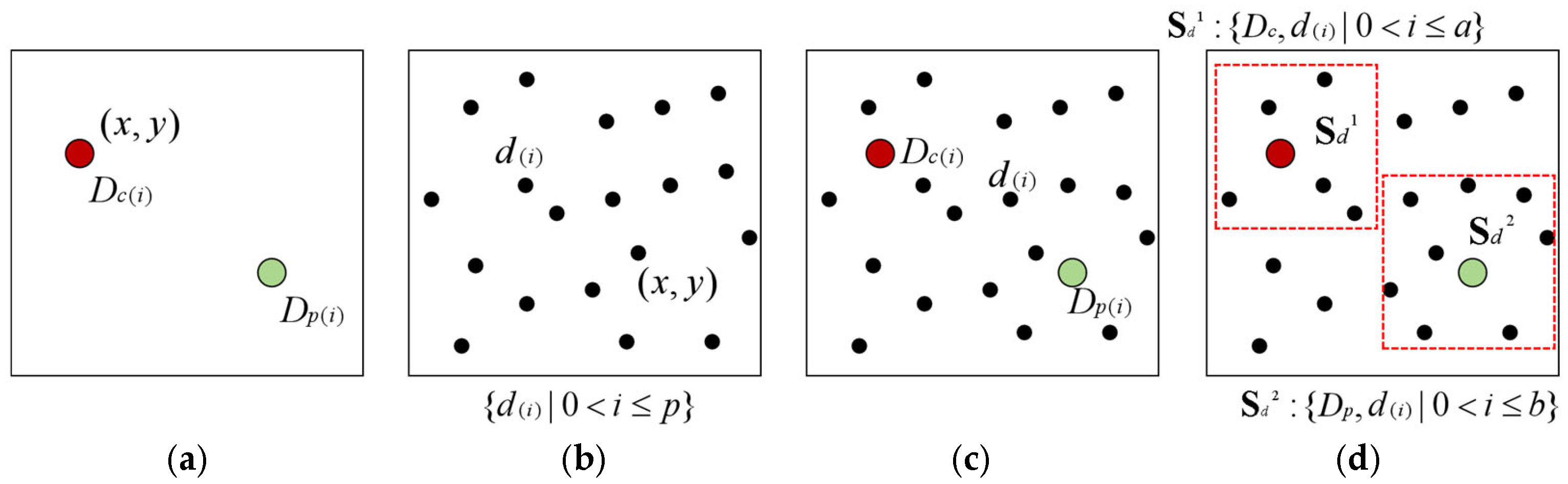
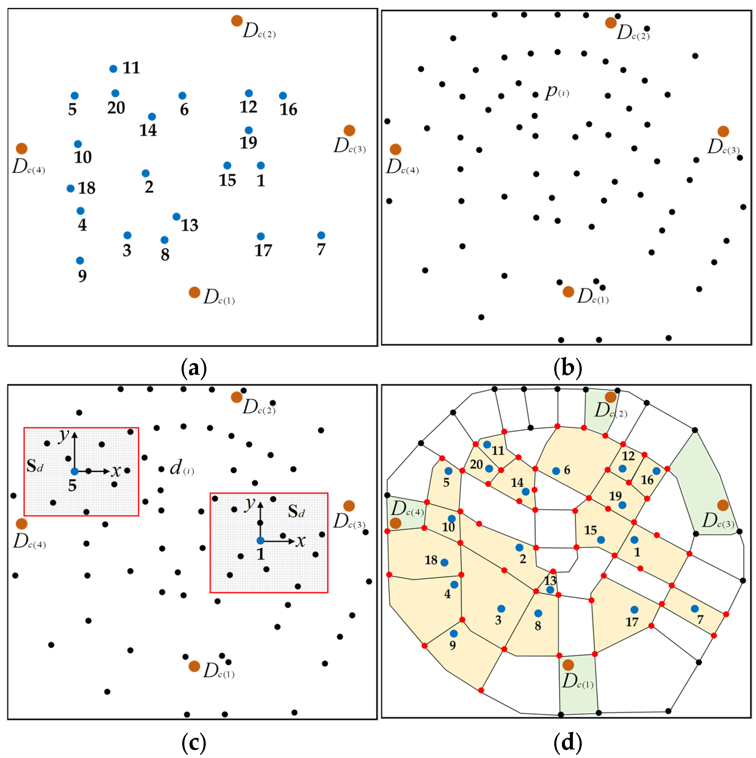
Definition 2.

Road node $d_{(i)}$ and local space $S_d$ of road node. The intersection point of two or more roads in a city is defined as a road node, denoted as $d_{(i)}$. If the number of road nodes relating to the cellular space construction extracted from the city is set to $p$, then there are $0<i\le p,i,p\in N$. The total $p$ number of road nodes constitutes the basic architecture of the entire urban cellular space. We select several road nodes $d_{(i)}$ within the collection $\{d_{(i)} | 0<i\le p\}$ in the neighborhood range of $D_{c(i)}$ and $D_{p(j)}$, with the distribution center $D_{c(i)}$ and delivery point $D_{p(j)}$ as the centers, respectively. If the neighborhood of $D_{c(i)}$ contains $a$ number of road nodes $d_{(i)}$, and the neighborhood of $D_{p(j)}$ contains $b$ number of road nodes $d_{(i)}$, then the neighborhood space composed of $D_{c(i)}$ and $a$ number of road nodes $d_{(i)}$ is defined as the local space $S_d$ of road nodes for the distribution center $D_{c(i)}$, denoted as $S_d:\{D_c,d_{(i)} | 0<i\le a\}$. The neighborhood space composed of $D_{p(j)}$ and $b$ number of road nodes $d_{(i)}$ is defined as the local space $S_d$ of road nodes for delivery point $D_{p(j)}$, denoted as $S_d:\{D_p,d_{(i)} | 0<i\le b\}$. Figure 2 shows the process of determining the local space $S_d$ of distribution center $D_{c(i)}$ and delivery point $D_{p(j)}$ from the urban road node space $\{d_{(i)} | 0<i\le p\}$. Figure 2a shows the positioning of the distribution center $D_{c(i)}$ and the delivery point $D_{p(j)}$. Figure 2b shows the set of road nodes. Figure 2c shows the spatial relationship between the distribution center, the delivery point, and the set of road nodes. Figure 2d shows the constructed local space ${S_d}^1$ of the distribution center $D_{c(i)}$ and local space ${S_d}^2$ of the delivery point $D_{p(j)}$.

Definition 3.

The spatial cellular $S_{(i)}$, the cellular control point $c_{(i)}$, and the cellular boundary $E_{(i)}$. The mathematical term “spatial cellular” originates from the concept of cellular automata in geographic information technology. It is used to describe the microscopic spatial structure that contains certain geographic entities. It divides the global geographic space in an orderly manner according to certain rules, realizing the quantification and regularization of the geographic space. According to the mathematical term, the closed micro-space containing the distribution center $D_{c(i)}$ or the delivery point $D_{p(j)}$ generated by searching for road nodes $d_{(i)}$ in local space $S_d$ is defined as a spatial cellular, denoted as $S_{(i)}$, in which the cellular containing distribution center $D_{c(i)}$ is denoted as $S_{c(i)}$, and the cellular containing delivery point $D_{p(j)}$ is denoted as $S_{p(j)}$. Define the road node $d_{(i)}$ that makes up the spatial cellular $S_{(i)}$ as the cellular control point, denoted as $c_{(i)}$, $0<i\le k$, $i,k\in N$. In the process of constructing a cellular model, the road connecting the adjacent control points $c_{(i)}$ and $c(i+1)$ is defined as the cellular boundary, denoted as $E_{(i)}$. According to the $k$ number of control points $c_{(i)}$, the corresponding number of cell boundaries $E_{(i)}$ is $k$; that is, for the presence of $E_{(i)}$, there is $0<i\le k$, $i,k\in N$.

According to the definition, there are the following constraint relationships between the spatial cellulars, the control points and the cell boundaries:

(1) The number of the control points $k$ meets $2<k\le a$ or $2<k\le b$, $k,a,b\in \mathrm{N}$;

(2) Point $D_{c(i)}$ or $D_{p(j)}$ does not intersect with any boundary $E_{(i)}$;

(3) There is only one nucleus $D_{c(i)}$ or $D_{p(j)}$ within the cellular;

(4) Send ray $l$ in any direction from the point $D_{c(i)}$ or $D_{p(j)}$ outward, and the number of the intersection point between $l$ and the cellular boundary $E_{(i)}$ must be odd;

(5) The area $S$ of the cellular region composed of control points $c_{(i)}$ must be the minimum value $\min S$;

(6) The cellular $S_{(i)}$ must be a convex polygon.

Definition 4.

The cellular searching coordinate system $xoy$, the cellular searching azimuth $\omega$, and the closed micro-space searching area $S_{[x,y,etal]}$. The coordinate system $xoy$ constructed by the cellular center point $D_{c(i)}$ or $D_{p(j)}$ as the coordinate origin is defined as the cellular searching coordinate system, which is used to search and determine the cellular control point $c_{(i)}$ and the cellular boundary $E_{(i)}$. Starting from the coordinate axis $y$, rotate the direction line $l_{(x,y)}$ clockwise according to the angular velocity $\Delta \omega$. When a node $d_{(i)}$ is searched, the angle between the direction line $l_{(o,d(i))}$ and the coordinate axis $y$ is defined as the cellular searching azimuth $\omega$. Searching for the nodes $d_{(i)}$, $d_{(i+1)}$, …, $d_{(j)}$, and the coordinate origin $o$, the nodes $d_{(i)}$, $d_{(i+1)}$, …, $d_{(j)}$ form a closed area, whose square measure is defined as the closed micro-space searching area, denoted as $S_{[o,d_{(i)},\dots ,d_{(j)}]}$. To ensure that the cellular $S_{(i)}$ is a convex polygon, it is determined that during the searching process, when $\omega <\pi$, the $S_{[o,d_{(i)},\dots ,d(j)]}$ must be a convex polygon.

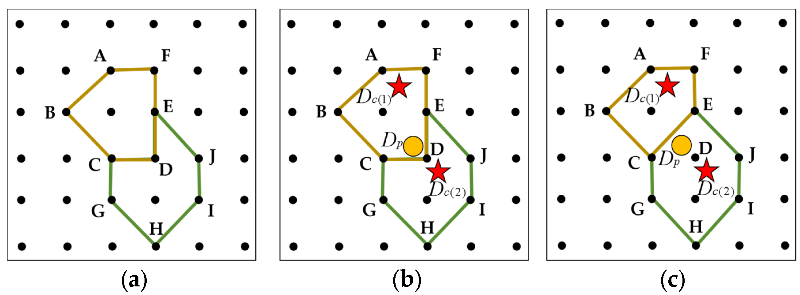
Here we prove that the constructed cellular must be constrained by the convex polygon:

(1) The spatial cellular constructs the attribution relationship between the distribution center $D_{c(i)}$ or delivery point $D_{p(j)}$ with the surrounding roads and road nodes, and the road nodes close to the center point should be included in the cellular scope;

(2) Hypothesis $H$: Allow a cellular to be a concave polygon, as shown in Figure 3a. The spatial layout contains both the convex polygon $S_{[ABCDEF]}$ and the concave polygon $S_{[CDEJIHG]}$. Figure 3b shows the spatial relationship between the convex polygon $S_{[ABCDEF]}$ and the concave polygon $S_{[CDEJIHG]}$ with the distribution center $D_{c_{(1)}}$, distribution center $D_{c(2)}$, and delivery point $D_p$, which is determined by the spatial cellular algorithm;

(3) Conclusion I: Judging from Figure 3b, there are three attribution relationships: $D_{c(1)}\in S_{[ABCDEF]}$, $D_p\in S_{[ABCDEF]}$, $D_{c(2)}\in S_{[CDEJIHG]}$. According to the definition, delivery point $D_p$ belongs to the cellular $S_{[ABCDEF]}$, thus, it is closer to $D_{c(1)}$ in the spatial relationship;

(4) Conclusion II: According to the spatial accessibility calculation model, it can be concluded that the straight-line distances between points satisfy $dis[D_{c(1)},D_p]>dis[D_{c(2)},D_p]$; thus, delivery point $D_p$ is closer to $D_{c(2)}$ in the spatial relationship;

(5) The above inference results indicate that there is a contradiction between Conclusion I and Conclusion II; therefore, hypothesis $H$ is not valid. It proves that the constructed cellular must be constrained by the convex polygon. The correct cellular structure is shown in Figure 3c, and both cellular $S_{[ABCEF]}$ and $S_{[CEJIHG]}$ are convex polygons.

Definition 5.

Empty cellular $S{(i)}^{Ø}$. Use the spatial cellular searching algorithm to obtain $m+n$ number of cellulars; if the $m+n$ number of cellulars cannot occupy all the urban space, then a cellular $S_{(i)}$ surrounded by the adjacent control points of a non-closed cellular that does not contain any point $D_{c(i)}$ or $D_{p(j)}$ is defined as an empty cellular, denoted as $S{(i)}^{Ø}$. Set the number of empty cellulars as $q$. Empty cellulars play a role in filling space in the quantification and regularization process of the urban geographic space. When the cellulars containing distribution centers or delivery points cannot be fully connected by road edges, or when the cellulars extend to the city boundary, the research scope cannot be fully covered; the empty cellulars will be used to fill the areas without distribution centers or delivery points, as well as the areas which are not covered by the city boundary. The empty cellulars ensure that the entire research scope of the city is covered by cellulars.

According to the definition, we construct an emergency logistics cellular space model based on the neighborhood topology algorithm.

Step 1: For the sample urban space, determine the main roads and $p$ number of road nodes $d_{(i)}$ of the city, and encode the main road nodes, $0<i\le p$. The urban spatial node set satisfies $\{d_{(i)} | 0<i\le p\}$.

Step 2: Determine the $m$ number of distribution centers $D_{c(i)}$ and $n$ number of delivery points $D_{p(j)}$ of the sample city. Take the arbitrary point $D_{c(i)}$ or $D_{p(j)}$ as a sample, then determine the local space $S_d$ of the sample point using the sets $S_d:\{D_c,d_{(i)} | 0<i\le a\}$ or $S_d:\{D_p,d_{(i)} | 0<i\le b\}$, and store the included nodes $d_{(i)}$ of $S_d$ in the Open List.

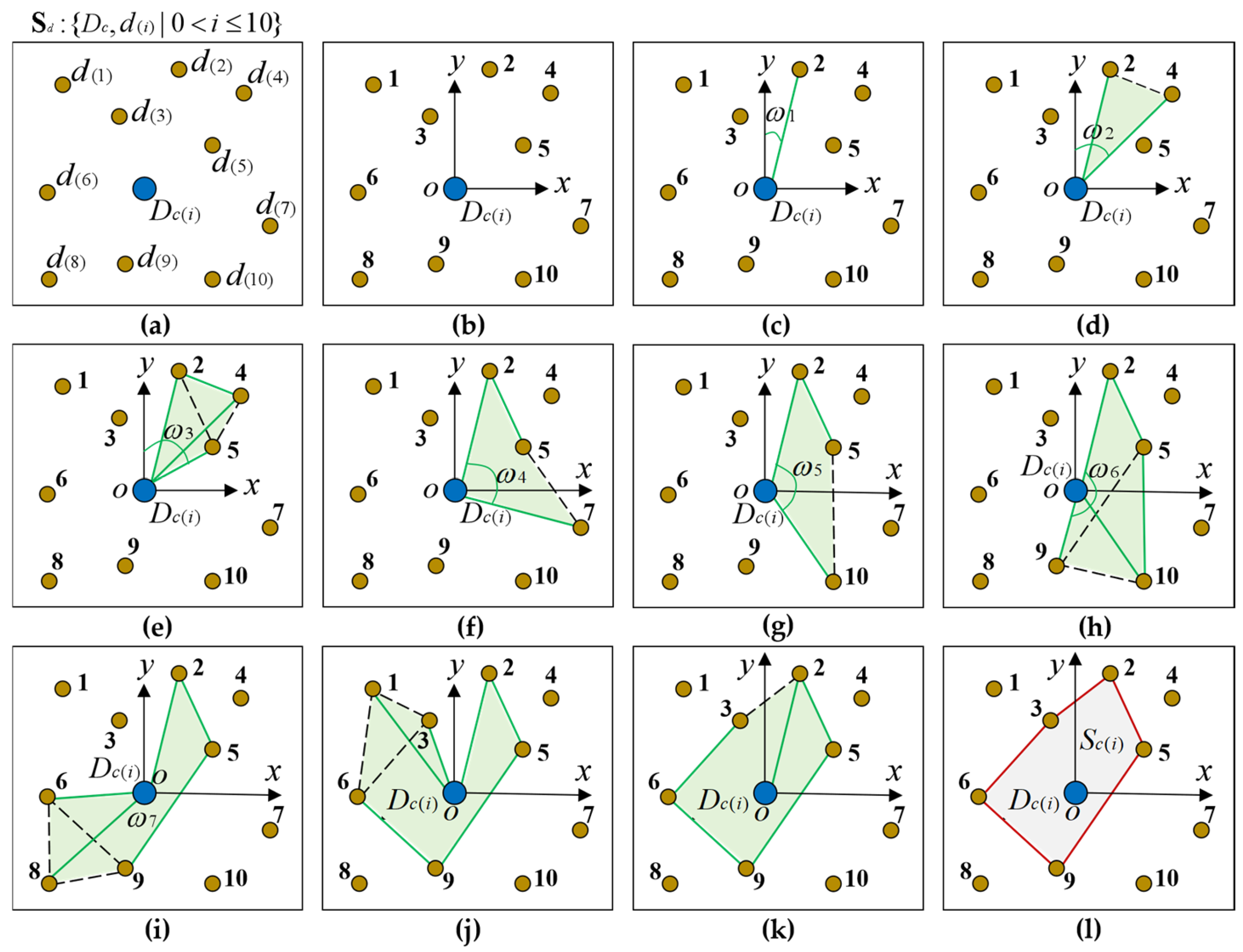
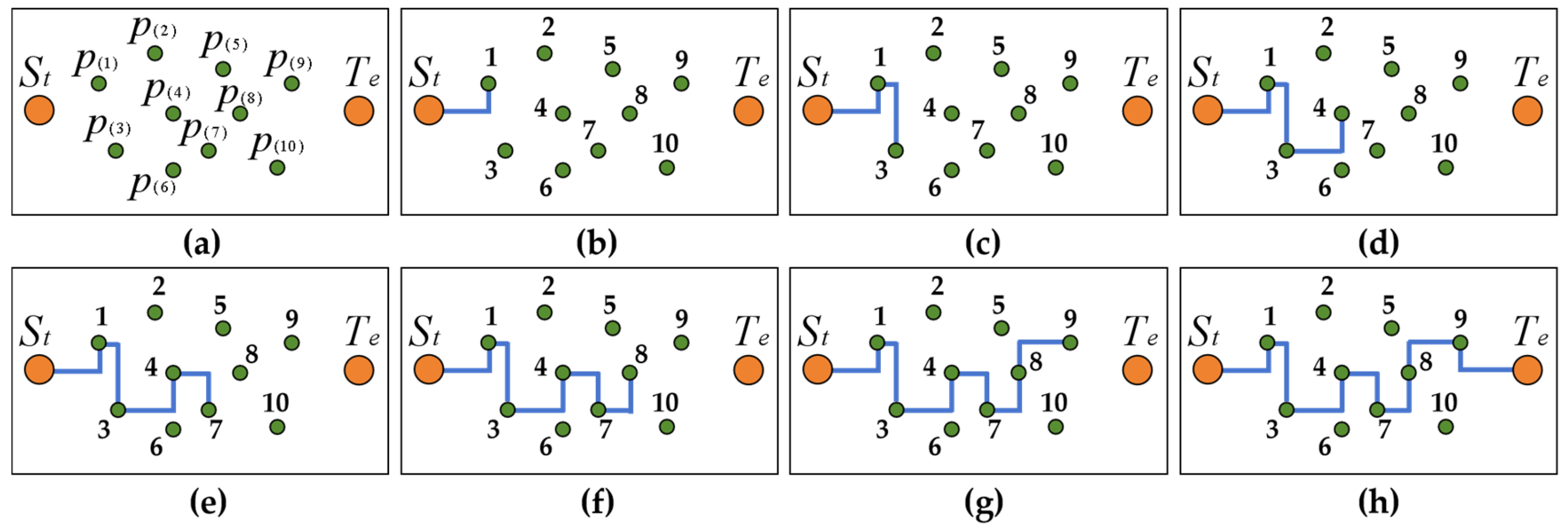
Step 3: Take the local space $S_d$ of the distribution center $D_{c(i)}$ as an example: $S_d:\{D_c,d_{(i)} | 0<i\le a\}$, as shown in Figure 4a. Build the cellular $S_{c(i)}$ where the distribution center $D_{c(i)}$ is located.

(1) Establish a coordinate system $xoy$ as shown in Figure 4b;

(2) The direction line $l_{(x,y)}$ searches at the angular velocity $\Delta \omega$, and $d_{(2)}$ is found at the azimuth angle ${\omega }_1$, as shown in Figure 4c. Determine that the $l_{(o,d_{(2)})}$ is feasible, store $d_{(2)}$ in the Closed List of the cellular $S_{c(i)}$, and delete it from the Open List;

(3) The direction line $l_{(x,y)}$ searches at the angular velocity $\Delta \omega$, and $d_{(4)}$ is found at the azimuth angle ${\omega }_2$, as shown in Figure 4d. Determine that the $l_{(o,d_{(4)})}$ is feasible, and $S_{(o,d_{(2)},d_{(4)})}$ is a feasible closed area. Store $d_{(4)}$ in the Closed List of $S_{c(i)}$ and delete it from the Open List;

(4) The direction line $l_{(x,y)}$ searches at the angular velocity $\Delta \omega$, and $d_{(5)}$ is found at the azimuth angle ${\omega }_3$, as shown in Figure 4e. Determine that $l_{(o,d_{(5)})}$ is feasible, and $S_{(o,d_{(2)},d_{(4)},d_{(5)})}$ is a feasible closed area. Continue to determine $S_{(o,d_{(2)},d_{(4)},d_{(5)})}>S_{(o,d_{(2)},d_{(5)})}$, delete $d_{(4)}$ from the Closed List, and retain $S_{(o,d_{(2)},d_{(5)})}$. Store $d_{(5)}$ in the Closed List of $S_{c(i)}$, and delete it from the Open List;

(5) The direction line $l_{(x,y)}$ searches at the angular velocity $\Delta \omega$, and $d_{(7)}$ is found at the azimuth angle ${\omega }_4$, as shown in Figure 4f. Judge that $S_{(o,d_{(2)},d_{(5)},d_{(7)})}$ is a concave quadrilateral, meaning it is not feasible. Abandon $d_{(7)}$, and continue searching;

(6) The direction line $l_{(x,y)}$ searches at the angular velocity $\Delta \omega$, and $d_{(10)}$ is found at the azimuth angle ${\omega }_5$, as shown in Figure 4g. Judge that $l_{(o,d_{(10)})}$ is feasible, and $S_{(o,d_{(2)},d_{(5)},d_{(10)})}$ is a feasible closed area. Store $d_{(10)}$ in the Closed List of $S_{c(i)}$ and delete it from the Open List;

(7) The direction line $l_{(x,y)}$ searches at the angular velocity $\Delta \omega$, and $d_{(9)}$ is found at the azimuth angle ${\omega }_6$, as shown in Figure 4h. Judge that $l_{(o,d_{(9)})}$ is feasible, and $S_{(o,d_{(2)},d_{(5)},d_{(10)},d_{(9)})}$ is a feasible closed area. Then, continue to determine the $S_{(o,d_{(2)},d_{(5)},d_{(10)},d_{(9)})}>S_{(o,d_{(2)},d_{(5)},d_{(9)})}$, delete $d_{(10)}$ from the Closed List, and retain $S_{(o,d_{(2)},d_{(5)},d_{(9)})}$. Store $d_{(9)}$ in the Closed List of $S_{c(i)}$, and delete it from the Open List;

(8) The direction line $l_{(x,y)}$ searches at the angular velocity $\Delta \omega$, and $d_{(8)}$ is found at the azimuth angle ${\omega }_7$, as shown in Figure 4i. Judge that $l_{(o,d_{(8)})}$ and $l_{(o,d_{(6)})}$ are feasible, and $S_{(o,d_{(2)},d_{(5)},d_{(9)},d_{(8)},d_{(6)})}$ is a feasible closed area. Then, continue to determine the $S_{(o,d_{(2)},d_{(5)},d_{(9)},d_{(8)},d_{(6)})}>S_{(o,d_{(2)},d_{(5)},d_{(9)},d_{(6)})}$. Store $d_{(6)}$ in the Closed List of $S_{c(i)}$, and delete it from the Open List;

(9) The direction line $l_{(x,y)}$ searches at the angular velocity $\Delta \omega$, and $d_{(1)}$ is found at the azimuth angle ${\omega }_9$, as shown in Figure 4j. Judge that $l_{(o,d_{(1)})}$ and $l_{(o,d_{(3)})}$ are feasible, and $S_{(o,d_{(2)},d_{(5)},d_{(9)},d_{(6)},d_{(1)},d_{(3)})}$ is a feasible closed area. Then, continue to determine the $S_{(o,d_{(2)},d_{(5)},d_{(9)},d_{(6)},d_{(1)},d_{(3)})}>S_{(o,d_{(2)},d_{(5)},d_{(9)},d_{(6)},d_{(3)})}$. Store $d_{(3)}$ in the Closed List of $S_{c(i)}$, and delete it from the Open List;

(10) The direction line $l_{(x,y)}$ searches at the angular velocity $\Delta \omega$, and when the $d_{(2)}$ is found, $S_{(o,d_{(2)},d_{(5)},d_{(9)},d_{(6)},d_{(3)})}$ satisfies all the constraints of $S_{(i)}$. It is feasible. Preserve the closed area $S_{(o,d_{(2)},d_{(5)},d_{(9)},d_{(6)},d_{(3)})}$ as the spatial cellular $S_{c(i)}$ of $D_{c(i)}$. At this time, the cellular contains the following:

① Cellular core: $D_{c(i)}$;

② Cellular control points: {$c_{(1)}$:$d_{(2)}$|$c_{(2)}$:$d_{(5)}$|$c_{(3)}$:$d_{(9)}$|$c_{(4)}$:$d_{(6)}$|$c_{(5)}$:$d_{(3)}$};

③ Cell boundary: {$E_{(1)}$:$E_{(d_{(2)},d_{(5)})}$|$E_{(2)}$:$E_{(d_{(5)},d_{(9)})}$|$E_{(3)}$:$E_{(d_{(9)},d_{(6)})}$|$E_{(4)}$:$E_{(d_{(6)},d_{(3)})}$|$E_{(5)}$:$E_{(d_{(3)},d_{(2)})}$};

④ Cellular region: $S_{(o,d_{(2)},d_{(5)},d_{(9)},d_{(6)},d_{(3)})}$.

Step 4: Construct the spatial cellulars for $m$ number of distribution centers and $n$ number of delivery points in the urban space by using the same searching algorithm as in Step 3. After the searching is completed, there are $m$ number of cellular $S_{c(i)}$ and $n$ number of cellular $S_{p(i)}$ in the urban space. The cellular spatial region $S_{total}$ satisfies Formula (1).

$$S_{total}\ge {\displaystyle \sum _{i=1}^m{S}_{c(i)}}+{\displaystyle \sum _{j=1}^n{S}_{p(j)}}$$

(1)

Step 5: When there is $S_{total}\ge {\displaystyle {\sum }_{i=1}^m{S}_{c(i)}}+{\displaystyle {\sum }_{j=1}^n{S}_{p(j)}}$, search for the nearest control nodes $c_{(i)}$ between the neighborhood cellular $S_{(i)}$ and $S_{(j)}$. Sequentially search and connect them to construct the empty cellular $S{(i)}^{Ø}$. Then, the cellular $S_{(i)}$, $S_{(j)}$ and the empty cellular $S{(i)}^{Ø}$ satisfy Formula (2).

$$S_{total}={\displaystyle \sum _{i=1}^m{S}_{c(i)}}+{\displaystyle \sum _{j=1}^n{S}_{p(j)}}+{\displaystyle \sum _{i=1}^{q}S{(j)}^{Ø}}$$

(2)

Step 6: Search the whole urban space till $S_{total}$ meets Formula (2). When the searching ends, output the cellular space.

3.1.2. Improved AGNES Clustering Algorithm Based on Cellular Space Model

The cellular space model constructs the spatial adjacency relationship between the distribution centers $D_{c(i)}$ and the delivery points $D_{p(j)}$, which includes the relationship with road nodes $d_{(i)}$ and road boundaries $E_{(i)}$. In the event of an emergency situation, determining the optimal distribution center $D_{c(i)}$ with the optimal spatial adjacency relationship is crucial for the points $D_{p(j)}$ that require material allocation, which can ensure the rapid delivery of materials to the designated locations $D_{p(j)}$. Based on the constructed cellular space model, the key issue is to determine the spatial neighborhood relationship between the distribution center cellular $S_{c(i)}$ and the delivery point cellular $S_{p(j)}$ in the cellular space. We use the decision tree algorithm to search for the spatially nearest neighborhood relationship and construct an improved AGNES clustering algorithm to determine the clustering relationship between the distribution centers $D_{c(i)}$ and the delivery points $D_{p(j)}$.

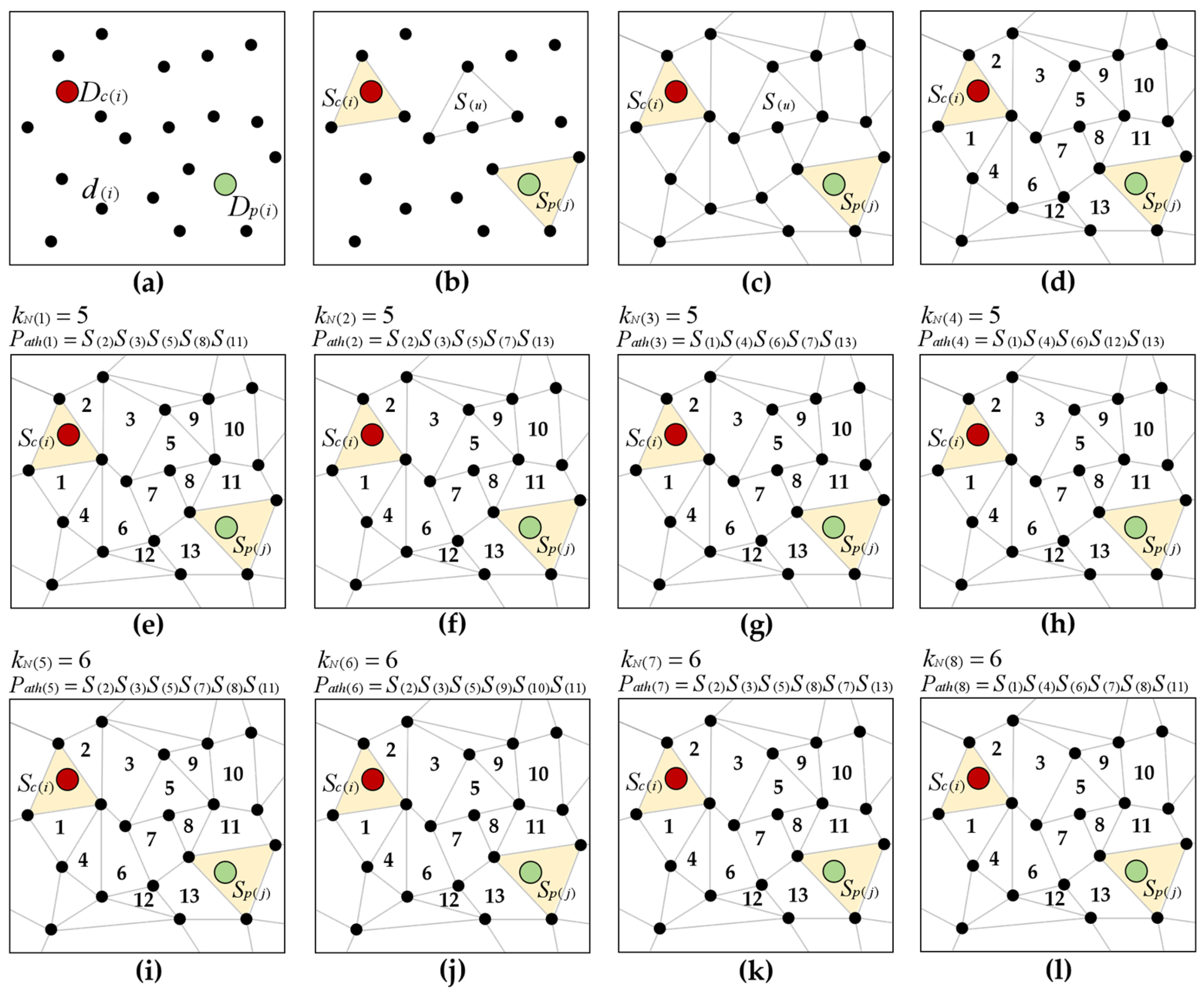
Definition 6.

The clustering target cellular $S_{N(i)}$, the number $k_{N(i)}$ of clustering target cellular, and the clustering target path $P_{ath(i)}$. Starting from arbitrary delivery point cellular $\forall S_{p(j)}$, search towards the direction of arbitrary distribution center cellular $\forall S_{c(i)}$, and sequentially search for the adjacent cellular $S_{(u)}$ and $S_{(v)}$ of the cellular $S_{p(j)}$ through the common edges $E_{(i)}$ until the adjacent cellular to the distribution center cellular $S_{c(i)}$ is found. The connection path formed by the cellulars along the way during the searching process is defined as the clustering target path, denoted as $P_{ath(i)}$. The adjacent cellular $S_{(u)}$ and $S_{(v)}$ on the clustering target path $P_{ath(i)}$ are uniformly defined as the clustering target cellulars, denoted as $S_{N(i)}$. Due to the complex adjacent relationship among cellulars in the cellular space, there may be $x$ number of paths $P_{ath(i)}$ from the delivery point cellular $S_{p(j)}$ to the distribution center cellular $S_{c(i)}$. Therefore, the number of clustering target cellulars found on a path $P_{ath(i)}$ is defined as $k_{N(i)}$, $0<i\le x$, $i,x\in N$. According to the definition, the clustering target cellular $S_{N(i)}$ on a path satisfies $0<i\le k_{N(i)}$, $i,k_{N(i)}\in N$. The clustering target cellular, the number of clustering target cellulars, and the clustering target path all describe the neighborhood relationship between the delivery point and the distribution center from the perspective of the cellular relationship that constitutes the spatial micro-structure. By determining the optimal target path and its corresponding target cellular number, the nearest path between the delivery point and the distribution center can be obtained, providing a data basis for constructing the clustering algorithm and the logistics route algorithm.

Figure 5 is the schematic diagram of generating the clustering target paths $P_{ath(i)}$ based on the distribution center $D_{c(i)}$, the delivery point $D_{p(j)}$, and the neighborhood cellular subspace. Figure 5a shows the spatial layout of the distribution center, the delivery point, and the road nodes. Figure 5b shows the generated distribution center cellular $S_{c(i)}$, the delivery point cellular $S_{p(j)}$, and the neighborhood cellular $S_{(u)}$. Figure 5c shows the generated cellular spatial sub-area. Figure 5d shows the potential cellulars with the codes that form the clustering target paths $P_{ath(i)}$ between the distribution center $D_{c(i)}$ and the delivery point $D_{p(j)}$. Figure 5e–h shows the four clustering target paths $P_{ath(1)}~P_{ath(4)}$ for the $k_{N(i)}=5$ number of clustering target cellulars. Figure 5i–l shows the four clustering target paths $P_{ath(5)}~P_{ath(8)}$ for the $k_{N(i)}=6$ number of clustering target cellulars.

Definition 7.

The clustering target adjacency index ${\delta }_{N(i)}$, the clustering target constraint factor ${\lambda }_{N(i)}$, and the clustering objective function $f_{(Dp(i),D_{c(i)})}$. Using arbitrary path $\forall P_{ath(i)}$ as the object, define the clustering target adjacency index as the reciprocal of the sum of the number $k_{N(i)}$ of clustering target cellulars on the path $P_{ath(i)}$ and the zero-suppression value 1, denoted as ${\delta }_{N(i)}$, as shown in Formula (3). In the geographic spatial constraints, if the coordinates of the distribution center $D_{c(i)}$ are $(x_{D_{c(i)}},y_{D_{c(i)}})$ and the coordinates of the delivery point $D_{p(i)}$ are $(x_{D_{p(i)}},y_{D_{p(i)}})$, then the spatial accessibility constructed by Formula (4) is defined as the clustering target constraint factor, denoted as ${\lambda }_{N(i)}$, in which $\sigma$ is the normalization factor. For the definition, ${\delta }_{N(i)}$ and ${\lambda }_{N(i)}$ satisfy $0<{\delta }_{N(i)}<1$, $0<{\lambda }_{N(i)}<1$, ${\delta }_{N(i)},{\lambda }_{N(i)}\in R^{+}$. The weighted mean of index ${\delta }_{N(i)}$ and factor ${\lambda }_{N(i)}$ is defined as the clustering objective function, as shown in Formula (5), in which the index ${\delta }_{N(i)}$ takes the maximum value of the index $\max {\delta }_{N(i)}$ corresponding to the path $P_{ath(i)}$ with the minimum number $k_{N(i)}$ of clustering target cellulars.

The clustering target adjacency index quantifies the close relationship between the distribution center and the delivery point by using the micro spatial structure of adjacent cellulars between the two points. The index value is determined by the number of adjacent cellulars. The clustering target constraint factor calculates the straight-line distance between the distribution center and the delivery point from the perspective of geographic accessibility, determining the close relationship between the two points. The clustering target adjacency index and the clustering target constraint factor are the data basis for constructing the spatial clustering relationship model between distribution centers and delivery points. The clustering objective function constructed by the two values is the key constraint condition for determining whether a delivery point belongs to the cluster in which the distribution center is located.

$${\delta }_{N(i)}={\displaystyle \frac{1}{k_{N(i)}+1}}$$

(3)

$${\lambda }_{N(i)}=\sigma \cdot {\displaystyle \frac{1}{\sqrt{{(x_{Dc(i)}-x_{Dp(i)})}^2+{(y_{Dc(i)}-y_{Dp(i)})}^2}}}$$

(4)

$$f(D_{p(i)},D_{c(i)})={\displaystyle \frac{\max {\delta }_{N(i)}+{\lambda }_{N(i)}}{2}}$$

(5)

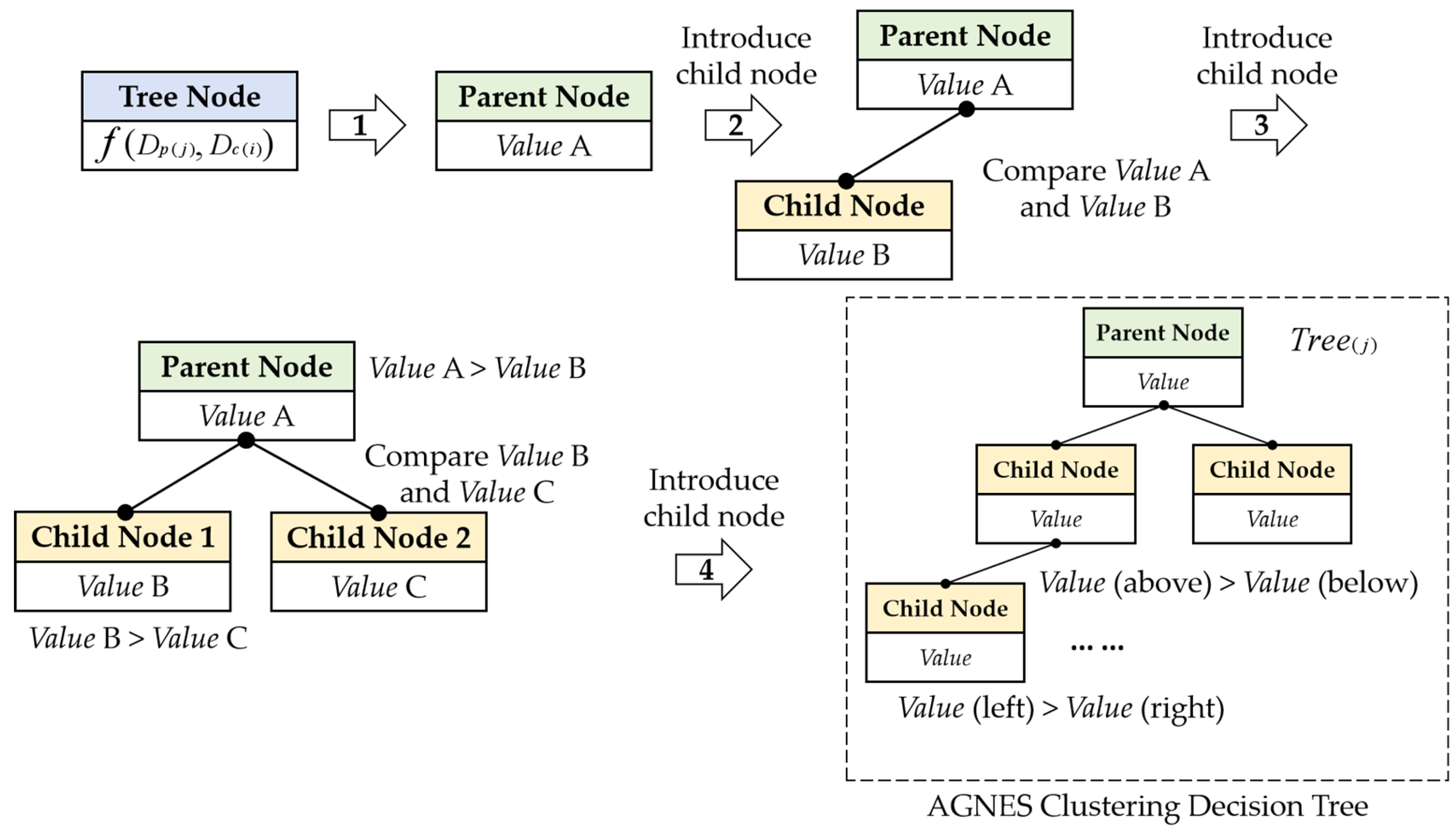
Definition 8.

AGNES clustering decision tree ${Tree}_{(j)}$. Search for the clustering objective functions $f(D_{p(j)},D_{c(i)})$ between the specified delivery point $D_{p(j)}$ and the $m$ number of distribution centers $D_{c(i)}$ in the cellular space, and store $m$ number of function values $f(D_{p(j)},D_{c(i)})$ in an orderly manner in the tree structure according to the rules of the complete binary tree algorithm. The constructed complete binary tree is defined as the AGNES clustering decision tree, denoted as ${Tree}_{(j)}$. The code $j$ of the tree $Tree(j)$ corresponds to the code of the delivery point $D_{p(j)}$, that is, one delivery point $D_{p(j)}$ corresponds to the construction of one decision tree $Tree(j)$. A complete binary tree is a computationally efficient tree structure that consists of a parent node and several child nodes, with all levels (except for the last level) fully filled and the nodes of the last level arranged as far to the left side as possible. When integrating the heap sorting algorithm, the global optimal solution can be finally classified into the parent node according to the binary tree searching algorithm. The process of obtaining the optimal solution is simple and efficient.

The tree node is defined as $T_{r(u,v)}$, in which $u$ represents the layer of the tree and $v$ represents the No. $v$ child node of the No. $u$ layer. Then the constructed decision tree ${Tree}_{(j)}$ satisfies the following conditions:

(1) Arbitrary node $T_{r(u,v)}$ can have a maximum of two child nodes $T_{r(u+1,*)}$ and a minimum of 0 child nodes;

(2) Arbitrary row $u$ of the $Tre{e}_{(i)}$ contains $2^{u-1}$ number of child nodes, $f(D_{p(j)},D_{c_{(1)}})$~$f(D_{p(j)},D_{c(m)})$ must be stored in the previous $m$ number of nodes, and then there is the following:

① The number of nodes that store $f(D_{p(j)},D_{c(i)})$ meets the requirement ${\displaystyle {\sum }_{u=1}^{\max u}{2}^{u-1}}\ge m$, $\max u$ representing the maximum row that can be stored currently;

② For any node $\forall T_{r(u,v)}$ that stores $f(D_{p(j)},D_{c(i)})$, its left node $T_{r(u,v-1)}$ must meet $T_{r(u,v-1)}\ne Ø$;

③ For any node $\forall T_{r(u,v)}$ that stores $f(D_{p(j)},D_{c(i)})$, its right node $T_{r(u,v+1)}$ satisfies the following:

(i) If the last $f(D_{p(j)},D_{c(m)})$ is currently stored in $T_{r(u,v)}$, the right node $T_{r(u,v+1)}$ does not exist;

(ii) If the current node $T_{r(u,v)}$ is not the last $f(D_{p(j)},D_{c(m)})$, the right node continues to store, satisfying the condition $T_{r(u,v+1)}\ne Ø$.

④ If row $u$ contains child nodes that store $f(D_{p(j)},D_{c(i)})$, then all nodes in the previous $u-1$ rows satisfy the condition $T_{r(u,v)}\ne Ø$.

(3) For any node $T_{r(u,v)}$: $T_{r(u,v)}$ stores $f(D_{p(j)},D_{c(i)})~f_{(1)}$ The child nodes $T_{r(u+1,2v-1)}$. and $T_{r(u+1,2v)}$ store $f_{(2)}$ and $f_{(3)}$; there must be $f_{(1)}\ge f_{(2)}\ge f_{(3)}$.

Definition 9.

AGNES clustering matrix $M_{(D_{p(j)})}$. Construct a $m\times p$ dimensional matrix to store the delivery points $D_{p(j)}$ output by the clustering algorithm. Define this matrix as the AGNES clustering matrix, denoted as $M_{(D_{p(j)})}$, in which $m$ represents the number of rows and $p$ represents the number of columns in the matrix, $m,p\in N$. To construct the AGNES clustering algorithm, we specify that the matrix $M_{(D_{p(j)})}$ satisfies the following constraints:

(1) Any row $\forall i$ corresponds to storing one cluster $c_{(i)}$, with each distribution center $D_{c(i)}$ being the cluster center. Store it in the first element of the No. $i$ matrix row.

(2) The number $m$ of rows in the matrix is equal to the number of clusters, then there is the following: $c_{(i)}$ corresponds to $D_{c(i)}$, $0<i\le m$, $i,m\in N$.

(3) The rows and columns of the matrix are full ranked, that is, ${rank(M_{(D_{p(j)})})}_{ro}=m$, ${rank(M_{(D_{p(j)})})}_{co}=p$.

(4) For row $\forall i$, the No. 2 to No. $p$ elements store the delivery points $D_{p(j)}$ of cluster $c_{(i)}$. The number $n_{(i)}$ of elements in the cluster $c_{(i)}$ satisfies $0<n_{(i)}\le p-1$, $n_{(i)},p\in N$.

Based on the above definitions, we construct an improved AGNES clustering algorithm based on the cellular space model as follows. Figure 6 shows the process of searching the AGNES clustering decision tree ${Tree}_{(j)}$ by using the algorithm.

Step 1: Construct a $m\times p$ dimensional matrix $M_{(D_{p(j)})}$. For the delivery point $D_{p(j)}$, take $j=1$. Take the distribution center $D_{c(i)}$ in the cellular space $S_{total}$:

(1) Take $i=1$, search for all clustering target paths $P_{ath(i)}$ and corresponding clustering target cellular number $k_{N(i)}$ between $D_{p(1)}$ and $D_{c(1)}$, and calculate the clustering target adjacency index ${\delta }_{N(1)}$;

(2) Search for coordinates $(x_{D_{p(1)}},y_{D_{p(1)}})$ of $D_{p(1)}$ and coordinates $(x_{D_{c(1)}},y_{D_{c(1)}})$ of $D_{c(1)}$, and calculate the clustering target constraint factor ${\lambda }_{N(1)}$;

(3) Calculate the clustering objective function $f(D_{p(1)},D_{c_{(1)}})$;

(4) Repeat steps (1) to (3), take $i=2$ and calculate $f(D_{p(1)},D_{c(2)})$;

(5) The $i$ traverses $0<i\le m$ and calculate $f(D_{p(1)},D_{c(i)})$. All $f(D_{p(1)},D_{c(i)})$ are recorded as $f{(i)}^{(1)}$, in which $i$ represents the No. $i$ distribution center $D_{c(i)}$, and number (1) represents $D_{p(1)}$.

Step 2: Construct a complete binary tree $Tre{e}_{\left(1\right)}$ with a total $m$ number of nodes, corresponding to the delivery point $D_{p\left(1\right)}$, and denote the tree node as $T_{r(u,v)}$. Store ${f\left(1\right)}^{\left(1\right)}$ in the parent node $T_{r\left(\mathrm{1,1}\right)}$. Take ${f\left(2\right)}^{\left(1\right)}$ and judge:

(1) If $f(1{)}^{\left(1\right)}\ge f(2{)}^{\left(1\right)}$, store ${f\left(2\right)}^{\left(1\right)}$ in child node $T_{r\left(\mathrm{2,1}\right)}$;

(2) If $f(1{)}^{\left(1\right)}<f(2{)}^{\left(1\right)}$, delete $T_{r\left(\mathrm{1,1}\right)}$, store ${f\left(2\right)}^{\left(1\right)}$ in $T_{r\left(\mathrm{1,1}\right)}$, store ${f\left(1\right)}^{\left(1\right)}$ in child node $T_{r\left(\mathrm{2,1}\right)}$.

Step 3: Take ${f\left(3\right)}^{\left(1\right)}$ and judge:

(1) If $f(1{)}^{\left(1\right)}\ge f(2{)}^{\left(1\right)}$:

① If $f(1{)}^{\left(1\right)}\ge f(2{)}^{\left(1\right)}\ge f(3{)}^{\left(1\right)}$, store ${f\left(3\right)}^{\left(1\right)}$ in child node $T_{r\left(\mathrm{2,2}\right)}$;

② If ${f\left(1\right)}^{\left(1\right)}\ge {f\left(3\right)}^{\left(1\right)}>{f\left(2\right)}^{\left(1\right)}$, delete $T_{r\left(\mathrm{2,1}\right)}$, store ${f\left(3\right)}^{\left(1\right)}$ in $T_{r\left(\mathrm{2,1}\right)}$, store ${f\left(2\right)}^{\left(1\right)}$ in child node $T_{r\left(\mathrm{2,2}\right)}$;

③ If ${f\left(3\right)}^{\left(1\right)}>{f\left(1\right)}^{\left(1\right)}\ge f{\left(2\right)}^{\left(1\right)}$, delete $T_{r\left(\mathrm{1,1}\right)}$ and $T_{r\left(\mathrm{2,1}\right)}$, store ${f\left(3\right)}^{\left(1\right)}$, ${f\left(1\right)}^{\left(1\right)}$ and ${f\left(2\right)}^{\left(1\right)}$ in $T_{r\left(\mathrm{1,1}\right)}$, $T_{r\left(\mathrm{2,1}\right)}$ and $T_{r\left(\mathrm{2,2}\right)}$.

(2) If $f(1{)}^{\left(1\right)}<f(2{)}^{\left(1\right)}$:

① If $f(3{)}^{\left(1\right)}\le f(1{)}^{\left(1\right)}<f(2{)}^{\left(1\right)}$, store ${f\left(3\right)}^{\left(1\right)}$ in child node $T_{r\left(\mathrm{2,2}\right)}$;

② If $f(1{)}^{\left(1\right)}<f(3{)}^{\left(1\right)}\le f(2{)}^{\left(1\right)}$, delete $T_{r\left(\mathrm{2,1}\right)}$, store ${f\left(3\right)}^{\left(1\right)}$ in $T_{r\left(\mathrm{2,1}\right)}$, store ${f\left(1\right)}^{\left(1\right)}$ in child node $T_{r\left(\mathrm{2,2}\right)}$;

③ If ${f\left(1\right)}^{\left(1\right)}<f{\left(2\right)}^{\left(1\right)}<{f\left(3\right)}^{\left(1\right)}$, delete $T_{r\left(\mathrm{1,1}\right)}$ and $T_{r\left(\mathrm{2,1}\right)}$, store ${f\left(3\right)}^{\left(1\right)}$, ${f\left(2\right)}^{\left(1\right)}$ and ${f\left(1\right)}^{\left(1\right)}$ in $T_{r\left(\mathrm{1,1}\right)}$, $T_{r\left(\mathrm{2,1}\right)}$ and $T_{r\left(\mathrm{2,2}\right)}$.

Step 4: Take $f{\left(i\right)}^{\left(1\right)}$, traverse $3<i\le m$. Compare the ${f\left(1\right)}^{\left(1\right)}$, ${f\left(2\right)}^{\left(1\right)}$, …, $f{\left(i\right)}^{\left(1\right)}$ by the same algorithm in Steps 2 to 3. According to the constraint conditions of the decision tree, store the ${f\left(1\right)}^{\left(1\right)}$, ${f\left(2\right)}^{\left(1\right)}$, …, $f{\left(i\right)}^{\left(1\right)}$ to the previous $i$ number of nodes in the tree $Tre{e}_{\left(1\right)}$. When $i=m$, $Tre{e}_{\left(1\right)}$ has been completely searched and output $Tre{e}_{\left(1\right)}$.

Step 5: Take the stored $f{\left(i\right)}^{\left(1\right)}$ in parent node $T_{r\left(\mathrm{1,1}\right)}$, and its corresponding distribution center $D_{c\left(i\right)}$ is the optimal distribution center for the entire tree $Tre{e}_{\left(1\right)}$.

Step 6: Search for the row $i$ corresponding to the distribution center $D_{c\left(i\right)}$ in the matrix $M_{\left(D_{p\left(j\right)}\right)}$, and store the delivery point $D_{p\left(1\right)}$ to the second element in the No. $i$ row.

Step 7: Return to Step 1; for the delivery point $D_{p\left(j\right)}$, take $j=2$. Build a complete binary tree $Tre{e}_{\left(2\right)}$ of the delivery point $D_{p\left(2\right)}$, search and output the optimal distribution center $D_{c\left(i\right)}$ corresponding to the parent node $T_{r\left(\mathrm{1,1}\right)}$. Store the delivery point $D_{p\left(2\right)}$ to the No. $j$ element in No. $i$ row. At this time, the elements of No. 1 to No. $j$ of the No. $i$ row are all non-zero ones.

Step 8: Traverse the code $j$ of the delivery points $D_{p\left(j\right)}$, $2<j\le n$. Construct a complete binary tree $Tre{e}_{\left(j\right)}$ of the delivery points $D_{p\left(j\right)}$ in sequence. For each tree, search and output the optimal distribution center $D_{c\left(i\right)}$ corresponding to the parent node $T_{r\left(\mathrm{1,1}\right)}$. Store the delivery point $D_{p\left(j\right)}$ to the No. $j$ element in No. $i$ row. At this time, the elements of No. 1 to No. $j$ of the No. $i$ row are all non-zero ones. When the searching of $j=n$ is completed, the algorithm ends. Output the AGNES clustering matrix $M_{\left(D_{p\left(j\right)}\right)}$ that meets the matrix constraint conditions.

3.2. Intelligent Emergency Logistics Route Model Based on Symmetrical Fruit Fly Optimization Algorithm

When major emergencies occur in a city, the vehicle traveling route for transporting materials from the distribution center to the delivery point is crucial. The core issue of emergency logistics is to construct routes with short transportation mileage, short time consumption, and low transportation costs. Based on the constructed urban cellular space and the clustering algorithm, and with the constraints of the urban geographic space as the modeling basis, we construct an urban emergency logistics route model based on an improved fruit fly optimization algorithm [17,18]. According to the symmetrical feature of logistics routes from one destination to another destination, the traveling distances within one route section are the same in both directions. Thus, if the logistics vehicles travel on one route section in different directions, the total route distance and costs will be the same. Based on this principle, the basic idea of modeling is as follows. Firstly, we determine $n$ number of delivery points to which materials need to be allocated. Then, we search for the cluster ${C_{\left(i\right)}}^{top}$ with the highest appearance frequency of $n$ number of delivery points, and select the distribution center $D_{c\left(i\right)}$ of the cluster as the starting point. If the $n$ number of delivery points appear in the same cluster, the distribution center of the cluster also serves as the terminal of the route. If the $n$ number of delivery points appear in different clusters, the cluster with the second-highest appearance frequency among $n$ number of delivery points is selected, and its distribution center $D_{c\left(i\right)}$ serves as the terminal of the route.

The fruit fly optimization algorithm is a relatively simple intelligent optimization algorithm that simulates the foraging mechanism of fruit fly groups searching for the optimal food location through their olfactory system, in order to search for the global optimal solution in the entire solution space [19,20]. Since searching for urban emergency logistics routes involves many road nodes and connecting roads, the constructed improved fruit fly optimization algorithm utilizes the route cost as the concentration factor for fruit fly individuals to search for food. The searching process of the algorithm is simulated as fruit fly foraging, and it can ultimately find the optimal solution [21].

Definition 10.

The route control point $p_{\left(i\right)}$, the route interval $S_{\left(i\right)}$, and the interval cost $c_{\left(i\right)}$. When designing the improved fruit fly optimization algorithm, the key road nodes or logistics nodes used to construct the traffic routes in the city are defined as the route control points, denoted as $p_{\left(i\right)}$. The interval formed by the movement of logistics vehicles from the control point $p_{\left(i\right)}$ to the adjacent control point $p_{(i+1)}$ connected by the urban road is defined as the route interval, denoted as $S_{\left(i\right)}$. Define the distance (unit: kilometer) traveled by the logistics vehicles from the point $p_{\left(i\right)}$ to the point $p_{(i+1)}$ as the interval cost, denoted as $c_{\left(i\right)}$. The encoding of each interval $S_{\left(i\right)}$ and interval cost $c_{\left(i\right)}$ is consistent with the encoding of the starting point $p_{\left(i\right)}$ of the interval.

Definition 11.

The fruit fly individual $F_{(i)}$, the fruit fly cost $C_{F\left(i\right)}$, and the fruit fly solution space $\mathbf{F}$. In the urban geographic space, the logistics vehicles depart from the starting point $p_{(i,0)}$ and pass through $x$ number of control points $p_{(i,1)}$, $p_{(i,2)}$, …, $p_{(i,x)}$, and finally reach the terminal $p_{(i,y)}$. The process of approaching the terminal forms a complete pathway, and the complete pathway composed of the starting point $p_{(i,0)}$, the control points $p_{(i,j)}$, and the terminal $p_{(i,y)}$ is defined as the fruit fly individual, denoted as $F_{(i)}$. According to the definition, when any control point $p_{(i,j)}$ in the pathway changes, a new fruit fly individual will be formed. The $F_{(i)}$ contains $x+2$ number of control points, forming a total of $x+1$ number of intervals $S_{\left(i\right)}$ and interval costs $c_{\left(i\right)}$. The complete route distance formed by the movement of logistics vehicles on the fruit fly individual $F_{(i)}$ is defined as the fruit fly cost, denoted as $C_{F\left(i\right)}$. According to the definition, we construct the fruit fly cost model, as shown in Formula (6). The solution set consisting of all fruit fly individuals formed by the control points $p_{\left(i\right)}$ for constructing the logistics routes in the urban geographic space is defined as the fruit fly solution space, denoted as $\mathbf{F}$.

$$C_{F\left(i\right)}=\sum _{i=1}^{x+1}{c}_{\left(i\right)}$$

(6)

Based on the above definitions, we construct the fruit fly individual searching algorithm, and the following is an example.

(1) Initialize the route interval $S_{\left(i\right)}$, including the starting point $S$, the ending point $T_e$, and several control points $p_{\left(i\right)}$, as shown in Figure 7a. Store $S_{\left(i\right)}$, $S_t$, $T_e$ and all $p_{\left(i\right)}$ in an Open List.

(2) Search in the direction to $T_e$ along the road, find point $p_{\left(1\right)}$, determine that it is feasible, and store it in the Closed List, as shown in Figure 7b;

(3) Continue searching for the point $p_{\left(3\right)}$, determine that it is feasible, and store it in the Closed List, as shown in Figure 7c;

(4) Continue searching for the point $p_{\left(4\right)}$, determine that it is feasible, and store it in the Closed List, as shown in Figure 7d;

(5) Continue searching. If the point $p_{\left(1\right)}$ is reached, points $p_{\left(1\right)}{p}_{\left(3\right)}{p}_{\left(4\right)}$ form a closed path, thus $p_{\left(1\right)}$ is discarded; search for point $p_{\left(2\right)}$; if the direction is opposite to the endpoint $T_e$, discard $p_{\left(2\right)}$; continue searching for the point $p_{\left(7\right)}$, determine that it is feasible, and store it in the Closed List, as shown in Figure 7e;

(6) Continue searching for the point $p_{\left(8\right)}$, determine that it is feasible, and store it in the Closed List, as shown in Figure 7f;

(7) Continue searching. If the point $p_{\left(4\right)}$ is reached, points $p_{\left(4\right)}{p}_{\left(7\right)}{p}_{\left(8\right)}$ form a closed path, thus $p_{\left(4\right)}$ is discarded; search for point $p_{\left(5\right)}$; if the direction is opposite to the endpoint $T_e$, discard $p_{\left(5\right)}$; continue searching for the point $p_{\left(9\right)}$, determine that it is feasible, and store it in the Closed List, as shown in Figure 7g;

Search for point $p_{\left(10\right)}$; if the direction is opposite to the endpoint $T_e$, discard $p_{\left(10\right)}$; continue searching, find $T_e$, then the searching process is finished. Output the fruit fly individual $F_{\left(i\right)}=S_t{p}_{\left(1\right),}{p}_{\left(3\right),}{p}_{\left(4\right),}{p}_{\left(7\right),}{p}_{\left(8\right),}{p}_{\left(9\right)}{T}_e$, as shown in Figure 7h.

Definition 12.

The food odor concentration $S_{F\left(i\right)}$ and the fitness function $f\left(S_{F\left(i\right)}\right)$. The fruit fly optimization algorithm aims to search for the fruit fly individual with the highest food odor concentration as the iterative objective, that is, to search for the optimal fruit fly individual. In the foraging behavior of a fruit fly group, when a fruit fly individual finds food with a certain odor concentration, other fruit flies will fly towards it and search for food along the way during the flight. If a fruit fly individual finds food with a higher odor concentration during the flight, all flies stop flying, and turn to the fruit fly individual with the higher odor concentration. This iteration continues until the fruit fly individual with the highest food odor concentration in the entire foraging space is found. Based on the logistics route targets, we suppose that the food odor concentration is generated by the fruit fly cost $C_{F\left(i\right)}$, and the lower the cost is, the higher the odor concentration will be. When outputting the fruit fly individual with the highest odor concentration in a certain iteration, the remaining fruit fly individuals will fly towards the optimal fruit fly individual. In the constructed algorithm, the directional flight is defined as the one-time replacement of control points $p_{(i,j)}$ in a fruit fly group. Construct a fitness function based on the food odor concentration, denoted as $f\left(S_{F\left(i\right)}\right)$. Formulas (7) and (8) represent the constructed food odor concentration $S_{F\left(i\right)}$ and fitness function $f\left(S_{F\left(i\right)}\right)$, in which $\zeta$ is the normalization factor.

$$S_{F\left(i\right)}={\displaystyle \frac{1}{C_{F\left(i\right)}}}$$

(7)

$$f(S_{F\left(i\right)})={\displaystyle \frac{1}{{\sum }_{i=1}^{x+1}{c}_{\left(i\right)}}}$$

(8)

Definition 13.

The current optimal fruit fly individual ${F_{\left(i\right)}}^{\Delta }$ and the fruit fly flight step size $S_{tep}(p_{\left(i\right)},p_{\left(j\right)})$. Randomly select arbitrary individual $\forall F_{\left(i\right)}$ from the fruit fly group as the target individual with the food odor concentration in the group searching, and define the selected fruit fly target individual as the current optimal fruit fly individual, denoted as ${F_{\left(i\right)}}^{\Delta }$. After selecting the ${F_{\left(i\right)}}^{\Delta }$, all other fruit fly individuals will fly towards ${F_{\left(i\right)}}^{\Delta }$ and continue to search for the better individuals during the flight. The process of a certain fruit fly individual $F_{(i)}$ flying towards the target individual ${F_{\left(i\right)}}^{\Delta }$ follows certain algorithmic rules. According to the definition and composition rules of the fruit fly individual $F_{(i)}$, it is agreed that the flight step size $S_{tep}(p_{\left(i\right)},p_{\left(j\right)})$ of the fruit fly individual is a neighborhood control point replacement of the corresponding route control points $p_{(i)}$ or a 2-opt operation of the logistics node $p_{(i)}$.

According to the definition, the process of a fruit fly individual $F_{\left(i\right)}$ flying towards ${F_{\left(i\right)}}^{\Delta }$ must go through $t\ge 1$ times of replacements of the control points or 2-opt operations. If the number of flights is $t$, then it will go through $t$ steps of flight. According to the definition, we construct a flight distance model for the fruit fly individual, as shown in Formula (9).

$$S_{tep}(F_{\left(i\right)},{F_{\left(i\right)}}^{\Delta })=\sum _{t=1}^{\max t}{S}_{tep}(p_{\left(i\right)},p_{\left(j\right)})$$

(9)

Based on the modeling approach, we divide the emergency logistics route model into two modules. (1) Module 1: Improved fruit fly optimization algorithm within the logistics sub-interval. The starting point and the ending point of the logistics sub-interval $I_{c\left(i\right)}$ are the adjacent distribution center $D_{c\left(i\right)}$ or the delivery point $D_{p\left(i\right)}$, respectively, and the control points $p_{\left(i\right)}$ within the sub-interval are road nodes. (2) Module 2: Improved fruit fly optimization algorithm within the logistics interval. The starting point of the logistics interval $I_{\left(i\right)}$ is a certain distribution center $D_{c\left(i\right)}$, and the ending point is the same distribution center $D_{c\left(i\right)}$ or the distribution center ${}^{\neg }D_{c\left(i\right)}{}_{\mathrm{}}$ in another cluster. The control point $p_{\left(i\right)}$ within the interval is the delivery point $D_{p\left(i\right)}$. According to the definition and modeling approach, we construct an urban emergency logistics route model based on an improved fruit fly optimization algorithm. The process is as follows. In the algorithm, we determine the starting point $D_{c\left(i\right)}$ and the ending point $D_{c\left(i\right)}$ of the logistics route, which includes $k$ number of delivery points $D_{p\left(i\right)}$ that require materials within the interval. Construct the sub-intervals by $D_{c\left(i\right)}$ and $D_{p\left(i\right)}$ and determine the set of road nodes within each sub-interval.

Algorithm Module one: Improved fruit fly optimization algorithm within the logistics sub-interval. Determine the optimal fruit fly individual and route cost for each sub-interval.

Step 1: Calculate the number $C(k,2)+k$ of sub-intervals based on the number $k$ of delivery points $D_{p\left(i\right)}$ and the starting and ending points $D_{c\left(i\right)}$.

Step 2: Take the first sub-interval $I_{c\left(i\right)}$, $i=1$, search for the optimal fruit fly individual ${F_{\left(i\right)}}^{opt}$ and corresponding fitness function $f(S_{F\left(i\right)}{)}^{opt}$ in the first sub-interval.

(1) Establish the road node set model for the sub-interval $I_{c^{\left(1\right)}}$, determine the starting point $S$, the ending point $T_e$, and several control points $p_{\left(i\right)}$;

(2) Initialize the fruit fly individual $F_{\left(i\right)}$ and the solution space $\mathbf{F}$. Set the solution space $\mathbf{F}$ to contain $x$ number of fruit fly individuals $F_{\left(i\right)}$, $0<i\le x$, $i,x\in \mathbf{N}$;

(3) Randomly select fruit fly individual $F_{\left(i1\right)}$ and determine it as the current optimal solution ${F_{\left(i1\right)}}^{\Delta }$, then calculate the individual fitness function as $f(S_{F\left(i1\right)}{)}^{\Delta }$;

(4) The remaining $x-1$ number of fruit fly individuals $F_{\left(i\right)}$ fly in a unit step $S_{tep}(p_{\left(i\right)},p_{\left(j\right)})$ towards ${F_{\left(i1\right)}}^{\Delta }$, and the following judgment is carried out:

① Execute one step size $S_{tep}(p_{\left(i\right)},p_{\left(j\right)})$; if the fitness functions $\forall f\left(S_{F\left(i\right)}\right)$ of all $x-1$ number of fruit fly individuals $F_{\left(i\right)}$ meet $\forall f\left(S_{F\left(i\right)}\right)\le f(S_{F\left(i1\right)}{)}^{\Delta }$, $0<i\le x-1$, and if $i\ne i_1$, then all $x-1$ number of fruit fly individuals $F_{\left(i\right)}$ continue to execute the second step size $S_{tep}(p_{\left(i\right)},p_{\left(j\right)})$ and compare $\forall f\left(S_{F\left(i\right)}\right)$ with $f(S_{F\left(i1\right)}{)}^{\Delta }$. If $\forall f\left(S_{F\left(i\right)}\right)\le f(S_{F\left(i1\right)}{)}^{\Delta }$ still exists, then continue to execute the third step size $S_{tep}\left(p_{\left(i\right),}{p}_{\left(j\right)}\right)$, and so on. Set the maximum step size to $h$.

② When all $x-1$ number of fruit fly individuals have been traversed after $h$ number of steps $S_{tep}(p_{\left(i\right)},p_{\left(j\right)})$, if there is still $\forall f\left(S_{F\left(i\right)}\right)\le f(S_{F\left(i1\right)}{)}^{\Delta }$, then the fruit fly individual $F_{\left(i1\right)}$ is the optimal individual ${F_{\left(i\right)}}^{opt}$, and the corresponding fitness function is the optimal solution $f(S_{F\left(i\right)}{)}^{opt}$. The searching ends.

③ During the step-size execution process, if a fruit fly individual $F_{\left(i2\right)}$ exists at No. $y$ step, $\exists f\left(S_{F\left(i2\right)}\right)>f(S_{F\left(i1\right)}{)}^{\Delta }$, the searching stops and returns to step (3). The fruit fly individual $F_{\left(i2\right)}$ becomes the current optimal solution ${F_{\left(i2\right)}}^{\Delta }$, and the individual fitness function $f(S_{F\left(i2\right)}{)}^{\Delta }$ is calculated. Continue with step (4).

④ Traverse all $x$ number of fruit fly individuals until there is a certain fruit fly individual $\exists F_{\left(id\right)}$, and if it satisfies $\exists f\left(S_{F\left(id\right)}\right)>\forall f\left(S_{F\left(i\right)}\right)$ compared to all the other $x-1$ number of fruit fly individuals $F_{\left(i\right)}$, then the searching ends and the fruit fly individual $F_{\left(id\right)}$ is output as the global optimal solution ${F_{\left(i\right)}}^{opt}$ in the sub-interval $I_{c^{\left(1\right)}}$, corresponding to the optimal fitness function $f(S_{F\left(i\right)}{)}^{opt}$.

Step 3: Take the second sub-interval $I_{c\left(i\right)}$, $i=2$, and search for the optimal fruit fly individual ${F_{\left(i\right)}}^{opt}$ and corresponding fitness function $f(S_{F\left(i\right)}{)}^{opt}$ in the second sub-interval.

Step 4: Traverse the sub-intervals $I_{c\left(i\right)}$, satisfy $2<i\le C(k,2)+k$, $i\in \mathbf{N}$, and search for the optimal fruit fly individual ${F_{\left(i\right)}}^{opt}$ and corresponding fitness function $f(S_{F\left(i\right)}{)}^{opt}$ in the No. $i$ sub-interval.

Step 5: The fitness function $f(S_{F\left(i\right)}{)}^{opt}$ within each sub-interval corresponds to the highest food odor concentration $S_{F^{\left(i\right)}}$ and the minimum route cost $C_{F\left(i\right)}$. Set the minimum cost for each sub-interval as $C_{F\left(i\right)}~C_{Ic\left(i\right)}$.

Algorithm Module 2: Improved fruit fly optimization algorithm within the logistics interval. Determine the optimal fruit fly individual and route cost within the logistics interval, and the cost between nodes is $C_{F\left(i\right)}~C_{Ic\left(i\right)}$.

Step 1: Calculate the number $A(k,k)$ of logistics intervals based on the number $k$ of delivery points $D_{p\left(i\right)}$ and the starting and ending points $D_{c\left(i\right)}$.

Step 2: Establish the node set model for the interval $I_{\left(i\right)}$, determine the starting point $D_{c\left(i\right)}$, the ending point $D_{c\left(i\right)}$, and $k$ number of delivery points $D_{p\left(i\right)}$.

Step 3: Initialize the fruit fly individual $F_{\left(i\right)}$ and the solution space $\mathbf{F}$. Suppose that the solution space $\mathbf{F}$ contains $x$ number of fruit fly individuals $F_{\left(i\right)}$, $0<i\le x$, $i,x\in \mathbf{N}$; according to actual conditions, there is $x=A(k,k)$.

Step 4: Randomly select fruit fly individual $F_{\left(i1\right)}$ and determine it as the current optimal solution ${F_{\left(i1\right)}}^{\Delta }$, calculate the individual fitness function as $f(S_{F\left(i1\right)}{)}^{\Delta }$.

Step 5: The remaining $x-1$ number of fruit fly individuals $F_{\left(i\right)}$ fly in a unit step $S_{tep}(p_{\left(i\right)},p_{\left(j\right)})$ towards ${F_{\left(i1\right)}}^{\Delta }$, and the following judgment is carried out:

(1) Execute one step size $S_{tep}(p_{\left(i\right)},p_{\left(j\right)})$; if the fitness functions $\forall f\left(S_{F\left(i\right)}\right)$ of all $x-1$ number of fruit fly individuals $F_{\left(i\right)}$ meet $\forall f\left(S_{F\left(i\right)}\right)\le f(S_{F\left(i1\right)}{)}^{\Delta }$, $0<i\le x-1$, and if $i\ne i_1$, then all $x-1$ number of fruit fly individuals $F_{\left(i\right)}$ continue to execute the second step size $S_{tep}(p_{\left(i\right)},p_{\left(j\right)})$ and compare $\forall f\left(S_{F\left(i\right)}\right)$ with $f(S_{F\left(i1\right)}{)}^{\Delta }$. If $\forall f\left(S_{F\left(i\right)}\right)\le f(S_{F\left(i1\right)}{)}^{\Delta }$ still exists, then continue to execute the third step size $S_{tep}(p_{\left(i\right)},p_{\left(j\right)})$, and so on. Set the maximum step size to $h$.

(2) When all $x-1$ number of fruit fly individuals have been traversed after $h$ number of steps $S_{tep}(p_{\left(i\right)},p_{\left(j\right)})$, if there is still $\forall f\left(S_{F\left(i\right)}\right)\le f(S_{F\left(i1\right)}{)}^{\Delta }$, then the fruit fly individual $F_{\left(i1\right)}$ is the optimal individual ${F_{\left(i\right)}}^{opt}$, and the corresponding fitness function is the optimal solution $f(S_{F\left(i\right)}{)}^{opt}$. The searching ends.

(3) During the step-size execution process, if a fruit fly individual $F_{\left(i2\right)}$ exists at No. $y$ step, $\exists f\left(S_{F\left(i2\right)}\right)>f(S_{F\left(i1\right)}{)}^{\Delta }$, the searching stops and returns to Step 4. The fruit fly individual $F_{\left(i2\right)}$ becomes the current optimal solution ${F_{\left(i2\right)}}^{\Delta }$, and the individual fitness function $f(S_{F\left(i2\right)}{)}^{\Delta }$ is calculated. Continue with Step 5.

(4) Traverse all $x$ number of fruit fly individuals until there is a certain fruit fly individual $\exists F_{\left(id\right)}$, and if it satisfies $\exists f\left(S_{F\left(id\right)}\right)>\forall f\left(S_{F\left(i\right)}\right)$ compared to all the other $x-1$ number of fruit fly individuals $F_{\left(i\right)}$, then the searching ends.

Step 6: The fruit fly individual $F_{\left(id\right)}$ is output as the global optimal solution ${F_{\left(i\right)}}^{opt}$ in the logistics interval $I_{\left(i\right)}$, corresponding to the optimal fitness function $f(S_{F\left(i\right)}{)}^{opt}$ and the lowest cost ${C_{\left(i\right)}}^{opt}$.

3.3. Sensitivity Analysis of the Algorithm

3.3.1. Sensitivity Analysis of the Improved AGNES Clustering Algorithm

The improved AGNES clustering algorithm realizes the cluster result that a delivery point $D_{p\left(i\right)}$ is included in a cluster of a certain distribution center $D_{c\left(i\right)}$, which is determined by the clustering objective function $f(D_{p\left(i\right)},D_{c\left(i\right)})$. The objective function is determined by the clustering target adjacency index ${\delta }_{N\left(i\right)}$ and the clustering target constraint factor ${\lambda }_{N\left(i\right)}$. According to Formulas (3)–(5), once the delivery point $D_{p\left(i\right)}$ and the target distribution center $D_{c\left(i\right)}$ are determined, their latitude and longitude coordinates are immediately confirmed, and then it is inferred that the ${\lambda }_N\left(i\right)$ is a fixed value. Therefore, the objective function is ultimately determined by the parameter $k_{N\left(i\right)}$ and is negatively correlated with $k_{N\left(i\right)}$. According to the analysis, the sensitivity of the improved AGNES clustering algorithm is directly related to the parameter $k_{N\left(i\right)}$. The sensitivity analysis is as follows:

(1) There are $x$ number of paths between the delivery point $D_{p\left(i\right)}$ and the target distribution center $D_{c\left(i\right)}$;

(2) Each path $P_{ath\left(i\right)}$ corresponds to $k_{N\left(i\right)}$ number of adjacent cellulars;

(3) In the clustering objective function $f(D_{p\left(i\right)},D_{c\left(i\right)})$, set $\max {\delta }_{N\left(i\right)}$ in the function structure, corresponding to $\min k_{N\left(i\right)}$;

(4) For any $\forall k_{N\left(j\right)}$, satisfy $\forall k_{N\left(j\right)}>\min k_{N\left(i\right)}$, $0<i,j\le x$, $i,j,x\in \mathbf{N}$;

(5) There must be $\max {\delta }_{N\left(i\right)}>\forall {\delta }_{N\left(j\right)}$, that is, $\max f(D_{p\left(i\right)},D_{c\left(i\right)})\left[i\right]>\forall f(D_{p\left(i\right)},D_{c\left(i\right)})\left[j\right]$, in which the subscript $\left[i\right]$ corresponds to the No. $i$ path, and the subscript $\left[j\right]$ corresponds to the No. $j$ path.

By analysis, it can be concluded that the sensitivity of the improved AGNES clustering algorithm is determined by the parameter $k_{N\left(i\right)}$ on the path $P_{ath\left(i\right)}$. Since the algorithm is designed with a fixed value ${\lambda }_{N\left(i\right)}$, the objective function is specifically influenced by $\max {\delta }_{N\left(i\right)}$. Therefore, the final calculation result of the objective function must be the maximum value among all paths $P_{ath\left(i\right)}$, which proves that $D_{p\left(i\right)}$ belongs to a certain cluster of $D_{c\left(i\right)}$ and does not belong to other clusters. The algorithm has strong stability.

3.3.2. Sensitivity Analysis of the Improved Fruit Fly Optimization Algorithm

The constructed improved fruit fly optimization algorithm is an optimization algorithm in two dimensions: in the logistics route sub-intervals and in the logistics route intervals. The determining parameter for the algorithm is the fruit fly cost $C_{F\left(i\right)}$, and the food odor concentration $S_{F\left(i\right)}$ and fitness function $f\left(S_{F\left(i\right)}\right)$ output by the algorithm are determined by $C_{F\left(i\right)}$. The sensitivity analysis of the algorithm is as follows:

(1) Any logistics sub-interval consists of a starting point $p_{(i,0)}$, $x$ number of road nodes $p_{(i,1)}$, $p_{(i,2)}$, …, $p_{(i,x)}$, and the endpoint $p_{(i,y)}$;

(2) Randomly select two road nodes $p_{(i,m)}$ and $p_{(i,n)}$, and the road distance of the traveling movement between the two nodes in the city is a constant value, that is, the interval cost $c_{\left(i\right)}$ is a constant value, $0<m,n\le x$, $m,n,x\in \mathbf{N}$;

(3) According to the fruit fly individual $F_{\left(i\right)}$ searching algorithm within the sub-interval, there are $x$ number of fruit fly individuals which are ultimately found by the step-size movement searching. Select the fruit fly individual corresponding to the minimum cost $\min C_{F\left(i\right)}$ as the sub-interval logistics distance, with the highest fitness function value $\max f\left(S_{F\left(i\right)}\right)$;

(4) Any logistics interval consists of $k$ number of delivery points and distribution centers $D_{c\left(i\right)}$ as the starting point and ending point. Since the sub-interval logistics distance between any two points is the minimum cost $\min C_{F\left(i\right)}$, which is a fixed value, according to the fruit fly individual $F_{\left(i\right)}$ searching algorithm within the interval, there are $x$ number of fruit fly individuals which are ultimately found by the step-size movement searching. Select the fruit fly individual corresponding to the minimum cost $\min {C_{F\left(i\right)}}^{total}$ as the interval logistics distance, with the highest fitness function value $\max f(S_{F\left(i\right)}{)}^{total}$.

It can be concluded that, for all the fruit flies in logistics sub-intervals and logistics intervals, the searching algorithm can ultimately find the optimal fruit fly individual within each logistics sub-interval and each logistics interval, corresponding to the route with the highest fitness function value. Due to the fixed road nodes in the city and the fixed distances of road traveling movement between points, when determining the starting point and ending point of the selected distribution centers as well as delivery points, the algorithm can ultimately find the optimal fruit fly with $\min C_{F\left(i\right)}$ in each sub-interval and the whole interval. Thus, the algorithm has strong stability.

4. Experimental Results and Analysis

To verify the feasibility and advantages of the proposed algorithm, we design experiments to test and validate the emergency logistics cellular space model based on the neighborhood topology algorithm, the improved AGNES clustering algorithm based on cellular space model, and the urban emergency logistics route model based on the improved fruit fly optimization algorithm. We also design a comparative experiment to demonstrate the advantages of the proposed algorithm. The basic idea of the experiment is as follows. Select Chengdu, the capital city of Sichuan Province in China, as the research scope. Take large supermarkets or commodity distribution centers as the experimental distribution centers, use the residential areas, hospitals, emergency shelters, hotels, etc., as the experimental delivery points. Select the number $m=4$ of representative distribution centers and number $n=20$ of delivery points within Chengdu city, and determine the geographic spatial coordinates $(x,y)$ of the distribution centers and the delivery points. Generate the cellular space and the spatial clusters by constructing algorithms. By determining the logistics sub-intervals and the logistics intervals, the improved fruit fly optimization algorithm is constructed to output the optimal logistics route. To verify the advantages of the proposed algorithm, we use the most commonly used algorithms for route planning, the Dijkstra algorithm and the A* algorithm, to output the optimal logistics routes under the same experimental conditions, and compare them with the proposed algorithm.

4.1. Data Collection

The collected data for the experiment are as follows:

(1) Collect data on the main roads and road nodes in the urban area of Chengdu as the research scope. In order to better fit the emergency logistics scenarios of main urban areas with large populations, we select areas with relatively dense urban road networks, and the road networks realize the full coverage of the geographical locations of distribution centers and delivery points. Therefore, based on the urban distribution structure, population density, and road spatial relationships of Chengdu, we select the urban areas within the Second Ring Road as the data collection scope.

(2) From the perspective of fairness in logistics distribution, when delivery points are evenly distributed within the research area, the selection of distribution centers should meet the fairness of geospatial layout, that is, the distribution centers should be located in relatively symmetrical positions in the spatial coordinate system. We divide the selected range into different quadrants of the spatial coordinate system and select the distribution centers along the Second Ring Road in the eastern, western, southern, and northern directions as the research objects, collecting a total of four distribution centers. Based on the analysis, we finally choose the following distribution centers: $D_{c\left(i\right)}$: {$D_{c\left(1\right)}$: Tiao San Ta; $D_{c\left(2\right)}$: He Hua Chi; $D_{c\left(3\right)}$: SM Square; $D_{c\left(4\right)}$: Guanghua Village}. Collect their latitude and longitude coordinates.

(3) The delivery point is another important research object and the core target of the clustering algorithm. Based on the emergency logistics scenario and the properties of the distribution objects, the selected delivery points for the experiment are locations that have high population concentrations and which would be in need of materials during major emergencies, such as residential areas, hospitals, schools, scenic spots, hotels, etc. Also, the selection of delivery points takes into account the fairness principle of the algorithm, which is positively correlated with the geographical layout of distribution centers and evenly distributed within the research area. In the experiment, we select hospitals, scenic spots, residential areas, hotels, etc. within the Second Ring Road as delivery points, which are evenly distributed and in line with the inherent logic of clustering algorithm. A total of 20 delivery points is collected along four directional lines in the city coordinate system. The delivery points are $D_{p\left(j\right)}$: {$D_{p\left(1\right)}$: No. 2 People’s Hospital; $D_{p\left(2\right)}$: People’s Park; $D_{p\left(3\right)}$: Jinguancheng Community; $D_{p\left(4\right)}$: Provincial Orthopedic Hospital; $D_{p\left(5\right)}$: Jinniu Community; $D_{p\left(6\right)}$: Chengdu Xinhua Hotel; $D_{p\left(7\right)}$: Shudu Garden Community; $D_{p\left(8\right)}$: Huaxi Hospital; $D_{p\left(9\right)}$: Luofu Family Community; $D_{p\left(10\right)}$: Provincial People’s Hospital; $D_{p\left(11\right)}$: Xijin International Plaza; $D_{p\left(12\right)}$: Workers’ Village Community; $D_{p\left(13\right)}$: Jinjiang Hotel; $D_{p\left(14\right)}$: Furong Hotel; $D_{p\left(15\right)}$: Crowne Plaza Hotel; $D_{p\left(16\right)}$: Ma’an East Road Community; $D_{p\left(17\right)}$: Shangri La Hotel; $D_{p\left(18\right)}$: Spring Garden Community; $D_{p\left(19\right)}$: Fangzheng Garden Community; $D_{p\left(20\right)}$: Jincheng Family Community}. Collect their latitude and longitude coordinates.

(4) Main roads, secondary roads, tertiary roads, and road nodes $d_{\left(i\right)}$ in the urban area of Chengdu. We take the Second Ring Road as the boundary. Firstly, we collect the main roads in Chengdu city, and then use the main roads as the skeleton to radiate around and collect the secondary roads. Then, we use the secondary roads as branches, and collect the tertiary roads connecting various distribution centers and delivery points to ensure that the main roads, secondary roads, and tertiary roads can cover all distribution centers and delivery points. After collecting the roads, we determine all road nodes. By collecting data from roads and road nodes, the research scope is discretized into a spatial architecture for the emergency logistics scenario, consisting of distribution centers, delivery points, multi-level roads, and road nodes.

(5) The experiment simulates a major emergency scenario within the research scope in which the delivery points urgently need supplies, for instance, large-scale water and power outages in cities, or sudden severe epidemics. It is necessary to select the neighborhood distribution centers as the starting and ending points from which the emergency management department allocates supplies. It is also necessary to construct an emergency logistics route that runs through the delivery points, with the goal of delivering urgently needed supplies to the delivery points with the shortest route and transportation time, and lowest costs, while meeting the basic living needs of urban residents.

(6) The emergency logistics scenario constructed in the experiment has the common properties of ordinary emergency logistics, including the correlation with the geographic spatial environment, the urban population distribution, and the basic needs of urban residents. In addition, it also includes the timeliness characteristics, that is, how to achieve the optimization of material distribution under the constraints of urban geographic space, how to minimize the transportation time and costs, and how to maximize the efficiency of emergency logistics.

4.2. Results and Analysis of Cellular Space Model

We use the constructed emergency logistics cellular space model based on the neighborhood topology algorithm to construct the cellular $S_{\mathrm{c}\left(i\right)}$ containing the distribution centers $D_{c\left(i\right)}$ and the cellular $S_{p\left(j\right)}$ containing the delivery points $D_{p\left(j\right)}$. Cellulars that do not include distribution centers and delivery points are empty cellular ${S_{\left(i\right)}}^{Ø}$. Figure 8 shows the cellular space result output by the proposed algorithm based on the original collected data. Figure 8a shows the extracted distribution centers $D_{c\left(i\right)}$ (brown dots) and the delivery points $D_{p\left(j\right)}$ (blue dots), with the number $j$ indicating the delivery point codes. Figure 8b shows the extracted road nodes (black dots). Figure 8c shows the extraction of the local space ${\mathbf{S}}_d$ of each delivery point in the road node set, with the red boundary area representing an example of the local space ${\mathbf{S}}_d$ of the delivery points $D_{p\left(1\right)}$ and $D_{p\left(5\right)}$. Figure 8d shows the output result of the cellular space, in which the green area represents the distribution center cellular $S_{\mathrm{c}\left(i\right)}$, the yellow area represents the delivery point cellular $S_{p\left(i\right)}$, the white area represents the empty cellular ${S_{\left(i\right)}}^{Ø}$, and the red dots on the boundary $E_{\left(i\right)}$ of the yellow cellular represent the cellular control points $c_{\left(i\right)}$.

Analyze the cellular space result output by the algorithm. The distribution centers and the delivery points extracted in Figure 8a are discretely distributed within the urban area of Chengdu, with relatively large distances. The selection of the distribution centers conforms to the logistics spatial relationship, that is, the distribution centers are generally located in the suburban areas with convenient transportation conditions. The selection of the delivery points is relatively uniform and distributed in the main areas of Chengdu, all of which are representative. Figure 8b shows the extracted key road nodes $d_{\left(i\right)}$. From the distribution of road nodes, the road nodes used to construct the cellulars are evenly distributed within the urban area of Chengdu, which meets the conditions for constructing the cellular space algorithm. Figure 8c conducts a local spatial ${\mathbf{S}}_d$ searching of road nodes for delivery points. Firstly, the cellular searching area for each delivery point is determined, and then the proposed algorithm is used to search and construct the cellulars. The selection of road nodes in local space ${\mathbf{S}}_d$ is based on the spatial micro-environment in which the delivery point is located, and is closely related to the quantity and distribution of the neighborhood road nodes $d_{\left(i\right)}$. Figure 8d shows the cellular space generated by the algorithm, which presents a coexistence condition of the distribution center cellulars, the delivery point cellulars, and the empty cellulars. The result shows that the distribution of each cellular is reasonable, and the distribution center cellular or delivery point cellular contains only one distribution center or delivery point, which conforms to the execution rules of the algorithm.

4.3. Results and Analysis of the Clustering

Based on the output results of the cellular space in Figure 8, we collect the spatial quantification relationships of the distribution center cellular $S_{\mathrm{c}\left(i\right)}$ and the delivery point cellular $S_{p\left(i\right)}$ separately, and calculate the clustering target adjacency index ${\delta }_{N\left(i\right)}$. Calculate the clustering target constraint factor ${\lambda }_N\left(i\right)$ based on the collected coordinates $(X_{D_c\left(i\right)},Y_{D_c\left(i\right)})$ of the distribution centers and $(X_{D_p\left(i\right)},Y_{D_p\left(i\right)})$ of the delivery points. Calculate the clustering objective function $f(D_{p\left(i\right)},D_{c\left(i\right)})$ based on the index ${\delta }_{N\left(i\right)}$ and the constraint factor ${\lambda }_N\left(i\right)$.

Table 1. The index ${\delta }_{N(i)}~\delta$, constraint factor ${\lambda }_N\left(i\right)~\lambda$, and objective function value $f(D_{p\left(i\right)},D_{c\left(i\right)})~f$ of each distribution point to the delivery center output by the algorithm.

	Dc(1)			Dc(2)			Dc(3)			Dc(4)
	$\delta$	$\lambda$	$f$	$\delta$	$\lambda$	$f$	$\delta$	$\lambda$	$f$	$\delta$	$\lambda$	$f$
$D_{p(1)}$	0.250	0.270	0.260	0.250	0.278	0.264	0.500	0.370	0.435	0.167	0.164	0.165
$D_{p(2)}$	0.250	0.323	0.286	0.200	0.222	0.211	0.167	0.185	0.176	0.500	0.294	0.397
$D_{p(3)}$	0.333	0.476	0.405	0.167	0.164	0.165	0.143	0.156	0.150	0.500	0.286	0.393
$D_{p(4)}$	0.333	0.294	0.314	0.143	0.167	0.155	0.125	0.139	0.132	0.500	0.476	0.488
$D_{p(5)}$	0.167	0.172	0.170	0.200	0.222	0.211	0.167	0.139	0.153	0.500	0.455	0.477
$D_{p(6)}$	0.200	0.208	0.204	0.500	0.400	0.450	0.333	0.222	0.278	0.167	0.227	0.197
$D_{p(7)}$	0.333	0.270	0.302	0.167	0.169	0.168	0.333	0.370	0.352	0.167	0.125	0.146
$D_{p(8)}$	0.500	0.714	0.607	0.167	0.164	0.165	0.167	0.175	0.171	0.333	0.238	0.286
$D_{p(9)}$	0.500	0.333	0.417	0.143	0.135	0.139	0.143	0.127	0.135	0.333	0.323	0.328
$D_{p(10)}$	0.200	0.222	0.211	0.167	0.196	0.181	0.143	0.143	0.143	0.500	0.588	0.544
$D_{p(11)}$	0.143	0.167	0.155	0.333	0.294	0.314	0.200	0.154	0.177	0.250	0.313	0.281
$D_{p(12)}$	0.200	0.196	0.198	0.500	0.500	0.500	0.333	0.345	0.339	0.143	0.164	0.153
$D_{p(13)}$	0.333	0.556	0.444	0.200	0.192	0.196	0.200	0.196	0.198	0.333	0.233	0.283
$D_{p(14)}$	0.200	0.233	0.216	0.333	0.303	0.318	0.200	0.192	0.196	0.250	0.278	0.264
$D_{p(15)}$	0.333	0.313	0.323	0.333	0.263	0.298	0.333	0.286	0.310	0.200	0.189	0.194
$D_{p(16)}$	0.200	0.182	0.191	0.333	0.455	0.394	0.500	0.476	0.488	0.143	0.145	0.144
$D_{p(17)}$	0.500	0.476	0.488	0.200	0.175	0.188	0.250	0.263	0.257	0.200	0.154	0.177
$D_{p(18)}$	0.250	0.256	0.253	0.143	0.167	0.155	0.125	0.135	0.130	0.500	0.625	0.563
$D_{p(19)}$	0.250	0.233	0.241	0.500	0.357	0.429	0.500	0.357	0.429	0.167	0.169	0.168
$D_{p(20)}$	0.167	0.192	0.179	0.250	0.278	0.264	0.167	0.164	0.165	0.333	0.333	0.333

shows the index ${\delta }_{N\left(i\right)}~\delta$, the constraint factor ${\lambda }_{N\left(i\right)}~\lambda$, and the objective function value $f(D_{p\left(i\right)},D_{c\left(i\right)})~f$ of each distribution point to the delivery center output by the algorithm.

Based on the output results in Table 1 and the proposed improved AGNES clustering algorithm, the results for the AGNES clustering decision tree ${Tree}_{(j)}$ are shown in Figure 9. Figure 9a–e shows decision trees $Tre{e}_{\left(1\right)}~Tre{e}_{\left(5\right)}$ of delivery points $D_{p\left(1\right)}~D_{p\left(5\right)}$. Figure 9f–j shows decision trees $Tre{e}_{\left(6\right)}~Tre{e}_{\left(10\right)}$ of delivery points $D_{p\left(6\right)}~D_{p\left(10\right)}$. Figure 9k–o shows decision trees $Tre{e}_{\left(11\right)}~Tre{e}_{\left(15\right)}$ of delivery points $D_{p\left(11\right)}~D_{p\left(15\right)}$. Figure 9p–t shows decision trees $Tre{e}_{\left(16\right)}~Tre{e}_{\left(20\right)}$ of delivery points $D_{p\left(16\right)}~D_{p\left(20\right)}$. Based on the results in Table 1 and Figure 9, output the AGNES clustering matrix $M_{(D_{p(j)})}$, as shown in

Table 2. The output AGNES clustering matrix $M_{(D_{p(j)})}$.

Cluster	Distribution Center	Element of the Cluster
$C_{(1)}$	$D_{c(1)}$	$D_{p(3)}$	$D_{p(8)}$	$D_{p(9)}$	$D_{p(13)}$	$D_{p(15)}$	$D_{p(17)}$
$C_{(2)}$	$D_{c(2)}$	$D_{p(6)}$	$D_{p(11)}$	$D_{p(12)}$	$D_{p(14)}$
$C_{(3)}$	$D_{c(3)}$	$D_{p(1)}$	$D_{p(7)}$	$D_{p(16)}$	$D_{p(19)}$
$C_{(4)}$	$D_{c(4)}$	$D_{p(2)}$	$D_{p(4)}$	$D_{p(5)}$	$D_{p(10)}$	$D_{p(18)}$	$D_{p(20)}$

.

Analyze the result data in Table 1. When using the distribution center as reference, each delivery point has different clustering target cellular numbers $k_{N\left(i\right)}$ as to the distribution center in the cellular space, resulting in significant differences in the calculated clustering target adjacency indices ${\delta }_{N\left(i\right)}$. The larger the index ${\delta }_{N\left(i\right)}$ is, the closer the adjacency relationship between the two cellulars in the cellular space will be, and the higher the probability of the delivery point being included in the cluster of the distribution center will be. Conversely, the lower the probability will be. The clustering target constraint factors ${\lambda }_N\left(i\right)$ calculated from the coordinates of the delivery points and the distribution centers also show significant differences. The larger the factor ${\lambda }_N\left(i\right)$ is, the shorter the distance between the two cellulars will be, and the higher the probability of a delivery point being included in the cluster of the distribution center will be. Conversely, the lower the probability will be. According to the calculated indices ${\delta }_{N\left(i\right)}$ and factors ${\lambda }_N\left(i\right)$, there are significant differences in the clustering objective function values $f(D_{p\left(i\right)},D_{c\left(i\right)})$. The larger the function value is, the higher the probability of the delivery point being included in the cluster of the distribution center will be, and vice versa. When using the delivery point as reference, the indices ${\delta }_{N\left(i\right)}$, the factors ${\lambda }_N\left(i\right)$, and the objective function $f(D_{p\left(i\right)},D_{c\left(i\right)})$ calculated between each delivery point and the four distribution centers are different, indicating that there are significant differences in the closeness, the spatial distance, and the clustering probability of the delivery points under the conditions of different distribution centers. The maximum value of the objective function is the cluster to which the delivery point belongs, indicating that the closeness, the spatial distance and the clustering probability values of the delivery point to the distribution center are all the highest.

The visualized AGNES clustering decision tree $Tre{e}_{\left(j\right)}$ in Figure 9 intuitively reflects the closeness relationship between the delivery points and various distribution centers. For a decision tree corresponding to a delivery point, it contains one parent node and three child nodes, and is the optimal complete binary tree. The parent node stores the highest objective function value, corresponding to the closest distribution center, which is also the cluster to which the delivery point belongs. Table 2 shows the clusters of the distribution centers based on the calculation results in Table 1 and the visualized AGNES clustering decision tree output in Figure 9. From analysis of the clustering result, the proposed algorithm can achieve uniform clustering of the delivery points in the urban cellular space. The maximum quantity of elements in clusters is six, and the minimum quantity of elements in clusters is four, which conforms to the distribution pattern and logistics layout of the delivery points and the distribution centers in the urban geographic space.

4.4. Results and Analysis of Logistics Routes

In the event of a sudden emergency, we select the set of delivery points that require supplies as: {$D_{p\left(1\right)}$, $D_{p\left(6\right)}$, $D_{p\left(10\right)}$, $D_{p\left(16\right)}$}. Based on the cluster of each delivery point, we determine the starting point $D_{c\left(3\right)}$ and the ending point $D_{c\left(2\right)}$ of the logistics route. Based on the set of the delivery points, the starting point, and the ending point, we construct each logistics sub-interval and logistics route interval, and construct the fruit fly individuals $F_{\left(i\right)}$, the fruit fly solution space $\mathbf{F}$, and the fruit fly costs $C_{F\left(i\right)}$ within each logistics sub-interval, then calculate the optimal food odor concentration $S_{F^{\left(i\right)}}$ and fitness function $S_{F^{\left(i\right)}}$ for each logistics sub-interval using the constructed module “improved fruit fly optimization algorithm within logistics sub-interval”. The results are shown in

Table 3. The food odor concentration ${S_{F(i)}}^{opt}$ and fitness function value $f(S_{F\left(i\right)}{)}^{opt}$ corresponding to the optimal fruit fly individual ${F_{\left(i\right)}}^{opt}$ in the logistics sub-interval.

Sub-Interval/Fruit Fly Individual F(i)	c3-p1	c3-p6	c3-p10	c3-p16	p1-p6	p1-p10	p1-p16
${S_{F(i)}}^{opt}$/$f(S_{F\left(i\right)}{)}^{opt}$	0.2564	0.1754	0.1124	0.3448	0.3448	0.1818	0.4348
Sub-interval/fruit fly individual $F_{(i)}$	p6-p10	p6-p16	p10-p16	c2-p1	c2-p6	c2-p10	c2-p16
${S_{F(i)}}^{opt}$/$f(S_{F\left(i\right)}{)}^{opt}$	0.2273	0.2273	0.1282	0.1724	0.2564	0.1493	0.2703

, in which “c3-p1” represents the sub-interval $D_{c\left(3\right)}{D}_{p\left(1\right)}$, “p1-p6” represents the sub-interval $D_{p\left(1\right)}{D}_{p\left(6\right)}$, and so on. Based on the fitness function values of the sub-intervals, the constructed module 2 “improved fruit fly optimization algorithm within logistics interval” is used to calculate and output the optimal food odor concentration $S_{F^{\left(i\right)}}$ and the fitness function $f\left(S_{F\left(i\right)}\right)$ for each logistics route. The results are shown in

Table 4. Food odor concentration $S_{F\left(i\right)}$ and fitness function $f\left(S_{F\left(i\right)}\right)$ of each route within the logistics interval.

Interval/Fruit Fly Individual F(i)	Sub-Interval/Fruit Fly Individual F(1)	Sub-Interval/Fruit Fly Individual F(2)	Sub-Interval/Fruit Fly Individual F(3)	Sub-Interval/Fruit Fly Individual F(4)	Sub-Interval/Fruit Fly Individual F(5)	Interval SF(i)/f(SF(i))
c3-1,6,10,16-c2	0.2564	0.3448	0.2273	0.1282	0.2703	0.0441
c3-1,6,16,10-c2	0.2564	0.3448	0.2273	0.1282	0.1493	0.0389
c3-1,10,6,16-c2	0.2564	0.1818	0.2273	0.2273	0.2703	0.0457
c3-1,10,16,6-c2	0.2564	0.1818	0.1282	0.2273	0.2564	0.0392
c3-1,16,6,10-c2	0.2564	0.4348	0.2273	0.2273	0.1493	0.0461
c3-1,16,10,6-c2	0.2564	0.4348	0.1282	0.2273	0.2564	0.0448
c3-6,1,10,16-c2	0.1754	0.3448	0.1818	0.1282	0.2703	0.0391
c3-6,1,16,10-c2	0.1754	0.3448	0.4348	0.1282	0.1493	0.0394
c3-6,10,1,16-c2	0.1754	0.2273	0.1818	0.4348	0.2703	0.0463
c3-6,10,16,1-c2	0.1754	0.2273	0.1282	0.4348	0.1724	0.0385
c3-6,16,1,10-c2	0.1754	0.2273	0.4348	0.1818	0.1493	0.0407
c3-6,16,10,1-c2	0.1754	0.2273	0.1282	0.1818	0.1724	0.0342
c3-10,1,6,16-c2	0.1124	0.1818	0.3448	0.2273	0.2703	0.0394
c3-10,1,16,6-c2	0.1124	0.1818	0.4348	0.2273	0.2564	0.0400
c3-10,6,1,16-c2	0.1124	0.2273	0.3448	0.4348	0.2703	0.0450
c3-10,6,16,1-c2	0.1124	0.2273	0.2273	0.4348	0.1724	0.0388
c3-10,16,1,6-c2	0.1124	0.1282	0.4348	0.3448	0.2564	0.0388
c3-10,16,6,1-c2	0.1124	0.1282	0.2273	0.3448	0.1724	0.0336
c3-16,1,6,10-c2	0.3448	0.4348	0.3448	0.2273	0.1493	0.0521
c3-16,1,10,6-c2	0.3448	0.4348	0.1818	0.2273	0.2564	0.0526
c3-16,6,1,10-c2	0.3448	0.2273	0.3448	0.1818	0.1493	0.0446
c3-16,6,10,1-c2	0.3448	0.2273	0.2273	0.1818	0.1724	0.0435
c3-16,10,1,6-c2	0.3448	0.1282	0.1818	0.3448	0.2564	0.0435
c3-16,10,6,1-c2	0.3448	0.1282	0.2273	0.3448	0.1724	0.0420

, in which “c3-1,6,10,16-c2” represents the starting point $D_{c\left(3\right)}$, the ending point $D_{c\left(2\right)}$, and the node order of the fruit fly individual, which is $D_{p\left(1\right)}$, $D_{p\left(6\right)}$, $D_{p\left(10\right)}$, $D_{p\left(16\right)}$.

Figure 10 shows the food odor concentration and fitness function value for each sub-interval based on the output data in Table 3. Figure 11 shows the food odor concentration and fitness function values for sub-intervals and the overall intervals of each route based on the output data in Table 4, with different colors representing different routes. Figure 11a shows the set of routes with the first delivery point $D_{p\left(1\right)}$, Figure 11b shows the set of routes with the first delivery point $D_{p\left(6\right)}$, Figure 11c shows the set of routes with the first delivery point $D_{p\left(10\right)}$, and Figure 11d shows the set of routes with the first delivery point $D_{p\left(16\right)}$. The horizontal axis numbers 1–5 in the figure represent the first to fifth sub-intervals of the route, and the number 6 represents the total interval of the route.

According to the calculation results in Table 3 and visualization results in Figure 10, the optimal fruit fly individuals within each logistics sub-interval are composed of different road nodes, resulting in different food odor concentrations and fitness functions. The calculation results in Table 3 represent the optimal food odor concentrations and fitness function values within the searched sub-intervals, showing a fluctuating trend in value. It indicates that when the logistics vehicles travel along the road nodes in the sub-intervals of the city, different logistics routes and costs will be generated due to factors such as the quantity of road nodes, the movement direction, and the node distance, which will finally affect the transportation costs of the entire logistics route. Among them, the sub-interval $D_{p\left(1\right)}{D}_{p\left(16\right)}$ has the highest odor concentration and a fitness function value of 0.4348, indicating that the logistics cost of this sub-interval is the lowest. The sub-interval $D_{c\left(3\right)}{D}_{p\left(10\right)}$ has the lowest odor concentration and a fitness function value of 0.1124, indicating that this sub-interval has the highest logistics cost. In the same sub-interval, due to the large quantity of road nodes, multiple fruit fly individuals could be generated. The experimental results prove that the proposed algorithm of module 1, “improved fruit fly optimization algorithm in logistics sub-interval”, can effectively find the optimal fruit fly individuals and the corresponding logistics routes in the sub-intervals; thus, the algorithm is feasible.

Analyzing the calculation results in Table 4 and visualization results in Figure 11, when using the fixed distribution center as the starting point and the ending point, the logistics interval contains the fruit fly individuals $F_{\left(i\right)}$ composed of multiple delivery points, resulting in different food odor concentrations and fitness functions. Table 4 lists the calculated global fruit fly individual data set, in which the same fruit fly individual is composed of the optimal fruit fly individuals from different sub-intervals, namely, each logistics route is sequentially connected by the optimal route within each logistics sub-interval. From the bar chart in Figure 11, it can also be concluded that different logistics routes have different sub-interval costs, corresponding to fluctuating food odor concentrations and fitness function values. The food odor concentrations and fitness function values within the sub-intervals show a fluctuating trend, and the food odor concentrations and fitness functions in the total intervals of the routes are also different. From analysis of the data in the last column of Table 4, the food odor concentrations and the fitness function values of the global fruit fly individuals show a trend of fluctuating in value, which is caused by the differences in the sub-interval structures of the fruit fly individuals, resulting in differences in the corresponding fruit fly individuals of the logistics routes. It indicates that when the logistics vehicles travel along the interval of the delivery points, they will be affected by the quantity of nodes, the movement direction, and the fitness function values of the sub-interval fruit fly individuals, generating different logistics routes and logistics costs, leading to the differences in food odor concentrations and fitness function values in the final output fruit fly group. Among them, the interval “c3-16,10,6-c2” has the highest odor concentration and a fitness function value of 0.0526, indicating that this interval has the lowest logistics cost. The logistics vehicles, starting from $D_{c\left(3\right)}$, pass through the delivery sequence of $D_{p\left(16\right)}$, $D_{p\left(1\right)}$, $D_{p\left(10\right)}$, $D_{p\left(6\right)}$, and finally return to $D_{c\left(2\right)}$, and the entire logistics route generates the lowest logistics cost. The interval “c3-10,16,1-c2” has the lowest odor concentration and a fitness function value of 0.0336, indicating that this interval has the highest logistics cost. The logistics vehicles, starting from $D_{c\left(3\right)}$, pass through the delivery sequence of $D_{p\left(10\right)}$, $D_{p\left(16\right)}$, $D_{p\left(6\right)}$, $D_{p\left(1\right)}$, and finally return to $D_{c\left(2\right)}$, and the entire logistics route generates the highest logistics cost. The experimental results prove that the proposed algorithm of module 2, “improved fruit fly optimization algorithm in logistics interval”, can effectively find the optimal fruit fly individual and its corresponding logistics route within the logistics interval; thus, the algorithm is feasible.

4.5. Comparative Experiment and Analysis

To verify the advantages of the proposed algorithm, we design and perform a comparative experiment. We select Dijkstra’s algorithm (DIA) and the A* algorithm (ASA), which are the most commonly used methods in logistics route planning, as the control group. At the same time, we set the proposed algorithm (PRA) as the experimental group. The conditions for the comparative experiment are as follows:

(1) Using the fitness function as the comparison parameter, compare the optimal fitness function values generated by the logistics sub-intervals and the logistics interval, respectively.

(2) The starting point is the distribution center $D_{c\left(3\right)}$, the ending point is the distribution center $D_{c\left(2\right)}$, and the delivery points are $D_{p\left(1\right)}$, $D_{p\left(6\right)}$, $D_{p\left(10\right)}$, and $D_{p\left(16\right)}$.

(3) Output the optimal fitness function value for each logistics sub-interval and the optimal fitness function value for each logistics interval by the experimental group and the control group, respectively.

(4) Compare the fitness function values between the control group and the experimental group in the logistics sub-intervals and the logistics intervals.

According to the content of the comparative experiment, the fitness function values of the logistics sub-intervals are output by using the control group DIA and ASA. The output results of the experimental group and the control group are shown in

Table 5. The output results of the optimal logistics sub-interval fitness function values by experimental group and control group.

PRA	Sub-interval/fruit fly individual $F_{(i)}$	c3-p1	c3-p6	c3-p10	c3-p16	p1-p6	p1-p10	p1-p16
	$f{(S_{F(i)})}^{opt}$	0.2564	0.1754	0.1124	0.3448	0.3448	0.1818	0.4348
	Sub-interval/fruit fly individual $F_{(i)}$	p6-p10	p6-p16	p10-p16	c2-p1	c2-p6	c2-p10	c2-p16
	$f{(S_{F(i)})}^{opt}$	0.2273	0.2273	0.1282	0.1724	0.2564	0.1493	0.2703
DIA	Sub-interval/fruit fly individual $F_{(i)}$	c3-p1	c3-p6	c3-p10	c3-p16	p1-p6	p1-p10	p1-p16
	$f{(S_{F(i)})}^{opt}$	0.2500	0.1493	0.0926	0.3226	0.3030	0.1639	0.3846
	Sub-interval/fruit fly individual $F_{(i)}$	p6-p10	p6-p16	p10-p16	c2-p1	c2-p6	c2-p10	c2-p16
	$f{(S_{F(i)})}^{opt}$	0.2083	0.2128	0.1136	0.1724	0.2222	0.1429	0.2439
ASA	Sub-interval/fruit fly individual $F_{(i)}$	c3-p1	c3-p6	c3-p10	c3-p16	p1-p6	p1-p10	p1-p16
	$f{(S_{F(i)})}^{opt}$	0.2273	0.1667	0.1000	0.2632	0.3030	0.1515	0.3704
	Sub-interval/fruit fly individual $F_{(i)}$	p6-p10	p6-p16	p10-p16	c2-p1	c2-p6	c2-p10	c2-p16
	$f{(S_{F(i)})}^{opt}$	0.2041	0.2174	0.1266	0.1563	0.2564	0.1220	0.2174

. Based on Table 5, we output the comparison results of each sub-interval in Figure 12a, in which the blue color represents PRA, the orange color represents DIA, and the green color represents ASA. Then, the DIA and ASA respectively output the optimal logistics route “c3-16,10,6-c2” and their corresponding fitness function values. The output results of the experimental group and the control group are shown in

Table 6. The fitness function values of the optimal logistics interval “c3-16,10,6-c2” output by the experimental group and control group.

	Sub-Interval/Fruit Fly Individual F(1)	Sub-Interval/Fruit Fly Individual F(2)	Sub-Interval/Fruit Fly Individual F(3)	Sub-Interval/Fruit Fly Individual F(4)	Sub-Interval/Fruit Fly Individual F(5)	Interval SF(i)/f(SF(i))
PRA	0.3448	0.4348	0.1818	0.2273	0.2564	0.0526
DIA	0.3226	0.3846	0.1639	0.2083	0.2222	0.0474
ASA	0.2632	0.3704	0.1515	0.2041	0.2564	0.0457

. Based on Table 6, we output the comparison results in Figure 12b, in which the blue color represents PRA, the orange color represents DIA, and the green color represents ASA. The horizontal axis numbers 1–5 in the figure represent the first to fifth sub-intervals of the route, and the number 6 represents the total interval of the route.

The following conclusions can be drawn from analysis of the calculation results in Table 5 and Table 6 as well as Figure 12. The fitness function value generated by PRA in each logistics sub-interval is higher than that of DIA and ASA, indicating that PRA has a lower route cost than DIA and ASA in each logistics interval. Compared with DIA, PRA has a maximum difference of 0.0502 within the sub-interval $D_{p\left(1\right)}{D}_{p\left(16\right)}$, indicating that PRA has the most obvious advantage in route searching within this sub-interval. Compared with ASA, PRA has a maximum difference of 0.0817 within the sub-interval $D_{c\left(3\right)}{D}_{p\left(16\right)}$, indicating that PRA has the most obvious advantage in route searching within this sub-interval. Analyzing the fitness function value of the optimal logistics interval “c3-16,10,6-c2”, we find that the fitness function values of PRA in both the logistics sub-intervals and the logistics interval are higher than those of DIA and ASA. Compared with DIA, PRA has a maximum fitness function value difference of 0.0502 in the logistics sub-interval $D_{p\left(16\right)}{D}_{p\left(1\right)}$, and, compared with ASA, PRA has a maximum difference of 0.0817 in the logistics sub-interval $D_{c\left(3\right)}{D}_{p\left(16\right)}$. For the overall fitness function value of the logistics route “c3-16,10,6-c2”, PRA is 0.0052 higher than DIA, with an optimization rate of 9.89%, while PRA is 0.0069 higher than ASA, with an optimization rate of 13.12%. The comparative experiment shows that our proposed algorithm has a higher fitness function value in the capacity of outputting the optimal logistics route compared to the traditional route planning algorithms, which corresponds to the lower logistics transportation costs. The comparative experiment verifies the advantages of our proposed algorithm.

To further verify the advantage of the experimental group algorithm, we use the t-test, from the significance test methods, to test the experimental group data and the control group data, as the sample size is small in the experiment. The starting point, delivery points, and endpoint of the logistics route are all consistent. The experimental group algorithm and the control group algorithm are used to output all feasible logistics routes, and the costs of all routes are shown in

Table 7. The total logistics route cost output by the experimental group and control group (unit: km).

Route	PRA	DIA	ASA	Route	PRA	DIA	ASA
c3-1,6,10,16-c2	22.7	25.0	25.1	c3-10,1,6,16-c2	25.4	29.0	29.1
c3-1,6,16,10-c2	25.7	27.8	28.4	c3-10,1,16,6-c2	25.0	28.7	27.8
c3-1,10,6,16-c2	21.9	23.7	25.1	c3-10,6,1,16-c2	22.2	25.6	25.5
c3-1,10,16,6-c2	25.5	28.1	27.4	c3-10,6,16,1-c2	25.8	28.7	28.6
c3-1,16,6,10-c2	21.7	23.1	24.8	c3-10,16,1,6-c2	25.8	30.0	27.8
c3-1,16,10,6-c2	22.3	24.7	23.8	c3-10,16,6,1-c2	29.8	33.4	32.2
c3-6,1,10,16-c2	25.6	29.0	28.4	c3-16,1,6,10-c2	19.2	20.8	22.9
c3-6,1,16,10-c2	25.4	28.4	28.1	c3-16,1,10,6-c2	19.0	21.1	21.9
c3-6,10,1,16-c2	21.6	24.3	24.8	c3-16,6,1,10-c2	22.4	24.2	26.5
c3-6,10,16,1-c2	26.0	28.7	27.9	c3-16,6,10,1-c2	23.0	24.5	26.3
c3-6,16,1,10-c2	24.6	27.1	28.1	c3-16,10,1,6-c2	23.0	25.8	25.5
c3-6,16,10,1-c2	29.2	32.1	31.5	c3-16,10,6,1-c2	23.8	25.8	26.3

. The number of route samples is n = 24, and the samples are independent. As seen in the data results in Table 7, the significance test (t-test) is conducted on PRA and DIA, and the same significance test (t-test) is conducted on PRA and ASA. Regarding the category of application scenario, logistics route planning belongs to the market application, and the data scale is relatively small. Thus, we set the commonly used significance level α = 0.05 and use a two-sided test. The results of the significance test (t-test) are shown in

Table 8. The results of the significance test (t-test).

Algorithm	Average Value	Variance	Standard Deviation	t Value	Significance Level	Degree of Freedom	Degree of Freedom (Critical Value)
PRA	24.025	6.958	2.638		α = 0.05	46	40 (−2.021)
DIA	26.650	9.930	3.151	−3.129			50 (−2.009)
ASA	26.825	5.992	2.448	−3.812			60 (−2.000)

. When comparing PRA with DIA, t = −3.129, and when comparing PRA with ASA, t = −3.812. When the degree of freedom is 46, the value of t is smaller than the critical value −2.021 for the degree of freedom 40 and the critical value −2.009 for the degree of freedom 50, both of which fall within the rejection domain. It indicates that PRA has a significant degree of difference from DIA and ASA, and PRA significantly reduces route costs compared to DIA and ASA, proving that our proposed algorithm is superior to DIA and ASA.

5. Conclusions

5.1. Conclusions of the Algorithm Research

In response to the research background and the existing problems of emergency logistics route planning in major urban emergencies, we construct an intelligent emergency logistics route model based on cellular space AGNES clustering and a symmetrical fruit fly optimization algorithm.

(1) For Research Question 1, we utilize the spatial relationships between the distribution centers, the delivery points, the urban roads, and the road nodes in the urban geographic space to construct a cellular algorithm based on the local space of road nodes, and then the entire urban logistics cellular space is constructed by designing a topology algorithm. By constructing the topology algorithm model, we determine the urban distribution centers, the delivery points, and the geographic spatial constraints, providing a prerequisite for establishing an emergency logistics route system in the city.

(2) For Research Question 2, based on the cellular space, an improved AGNES clustering algorithm is constructed to establish the spatial clustering relationship between the delivery points and the adjacent distribution centers, providing the spatial data foundation for designing the emergency logistics routes.

(3) For Research Question 3, we integrate the intelligent algorithm into the emergency logistics route planning, and construct an urban emergency logistics route model based on an improved fruit fly optimization algorithm. We conduct global searching of fruit fly individuals within the logistics sub-intervals to obtain the optimal fruit fly individuals and the optimal logistics routes. Based on this, we conduct global searching of the fruit fly individuals within the logistics interval to obtain the optimal fruit fly individual and the optimal logistics route, achieving the lowest-cost emergency logistics route planning. Experimental results show that our proposed algorithm can output the optimal logistics routes for each logistics sub-interval and the entire logistics interval. Compared with the traditional route planning methods of the Dijkstra algorithm and the A* algorithm, it can reduce the cost of route planning and achieve optimization rates of 9.89% and 13.12%, respectively. The t-test significance test proves that the constructed algorithm is superior to the traditional route planning algorithms in saving route costs.

5.2. The Significance of the Research Results in Emergency Management

The constructed intelligent emergency logistics route model is of great significance in urban emergency management. Firstly, the constructed cellular space model utilizes a quantitative research method to realize the relationship between distribution centers, delivery points, urban roads, and road nodes in the urban geographic space. It constructs the layout structure of the distribution centers and delivery points in the urban geographic space, providing decision-making support for emergency management departments to plan logistics routes, determine the priorities for material allocation, and judge the accessibility of delivery points. Secondly, we construct an AGNES clustering algorithm to establish the attribution relationship between the distribution centers and the neighborhood delivery points, which can help emergency management departments divide urban emergency logistics jurisdiction areas based on local regions and improve emergency management efficiency. Finally, based on the constructed spatial cellular and the AGNES clustering algorithm, we construct emergency logistics routes to plan the optimal distribution routes for emergency management departments, which can effectively save logistics costs and improve material distribution efficiency, thereby enhancing the operational and regulatory efficiency of emergency management departments. It provides decision-making solutions to ensure the smooth and orderly operation of the city and the normal living and working order of urban residents.

5.3. Discussion on the Algorithm’s Scalability

The constructed algorithm has strong portability and scalability. Firstly, when the urban area is set as the research range, the data bases and the modeling conditions for the constructed improved AGNES clustering algorithm and the fruit fly optimization algorithm are as follows:

(1) The distribution centers, delivery points, and road nodes distributed in the city;

(2) The geographic spatial coordinates of all the points;

(3) The distances of road traveling movement between points;

(4) The starting point and the ending point of the logistics vehicle;

(5) Determine the quantity of delivery points, and the specific delivery points for the required materials.

According to the characteristics of the urban geographic spatial structure, cities with different hierarchies or built-up areas can provide the above five data bases and modeling conditions. Therefore, the algorithm has strong portability and scalability, and it can be used for emergency logistics route planning in any city. When the algorithm is applied to cities with larger areas and higher hierarchies, there may be more distribution centers and delivery points in the city. The complexity of the urban road networks is higher, and the distances between points are greater; thus, the algorithm requires a larger amount of data and higher computational costs.

Secondly, we will further expand the coverage of emergency logistics routes. If a key city is used as the material distribution center and supplies are transported to satellite cities around the key city, the constructed algorithm is also applicable. Using the key city and several satellite cities as the entities distributed in the geographic space, the improved AGNES clustering algorithm could also be constructed to achieve the spatial clustering of the satellite cities and obtain their spatial closeness relationship. Then, starting from and ending at the key distribution city, and using the satellite cities in need of materials as the delivery points, an improved fruit fly optimization algorithm could also be constructed to search for the optimal logistics route. In this situation, the logistics sub-interval is the optimal path between two cities, and the logistics interval is the closed-loop route connecting all the satellite cities in need of materials with the key city.

5.4. Limitations and Future Work

5.4.1. Limitations of the Work

The constructed algorithm and the conducted experiment are based on the selected urban distribution centers and delivery points. The research objects are representative large shopping malls, residential areas, hospitals, hotels, etc., in the city. The selection of points is relatively fixed, and the selection of the distribution centers as the core research objects for the clustering algorithm is random. Meanwhile, the selection of logistics route delivery points is also random. Thus, the constructed method is a universal logistics route algorithm. As for more refined, personalized, and customized material distribution scenarios, the further research conditions, constraints, and applicable scenarios should be determined. In the work, the research scope is the main urban area of a city, and does not involve the satellite cities around the key city. Emergency material distribution and logistics route planning issues for the satellite cities are not considered, and this is also a direction for future research.

5.4.2. Future Work

The constructed algorithm is based on distribution centers and delivery points with fixed geographical locations. The complex road relationships and node layouts in the urban geographic space have direct constraints on the planning of logistics routes. In future work, we will conduct further research on the following three aspects.

Firstly, the selected distribution centers for the algorithm’s modeling are representative large-scale supermarkets or material sales points in the city. There are a large number of large supermarkets and material sales points in cities, which are distributed in different geographical locations. Therefore, building a location selecting model for the distribution centers is another research field to further optimize the emergency logistics route algorithm. It is necessary to establish the logistics demand scenarios for delivery points and construct the algorithm based on the geospatial constraints.

Secondly, in the context of emergency situations, each delivery point has different quantity demands and urgency levels for the required materials. Determining the priority of the delivery points based on the different material quantity demands and urgency levels, and then determining the order of the logistics routes according to the priority of the delivery points, is another research field in constructing the logistics route algorithm with different factors as constraints. It is necessary to combine the levels of delivery points and the material allocation demand scenarios, as well as the geospatial constraints to construct the route algorithm.

Thirdly, we will expand our research scope and further study the emergency logistics route algorithm in cross-city or cross-regional scenarios. Using the key city as the distribution center and the surrounding satellite cities as delivery points, we will construct a spatial clustering algorithm to achieve satellite city clustering. Then, starting from the key city, we will study the improved fruit fly optimization algorithm for the satellite cities, achieving the cross-city and cross-regional distribution of emergency supplies.