Optimal Energy-Aware Scheduling of Heterogeneous Jobs with Monotonically Increasing Slot Costs

Abstract

Energy-aware scheduling plays a critical role in modern computing and manufacturing systems, where energy consumption often increases with job execution order or resource usage intensity. This study investigates a scheduling problem in which a sequence of heterogeneous jobs—classified as either heavy or light—must be assigned to multiple identical machines with monotonically increasing slot costs. While the machines are structurally symmetric, the fixed job order and cost asymmetry introduce significant challenges for optimal job allocation. We formulate the problem as an integer linear program and simplify the objective by isolating the cumulative cost of heavy jobs, thereby reducing the search for optimality to a position-based assignment problem. To address this challenge, we propose a structured assignment model termed monotonic machine assignment, which enforces index-based job distribution rules and restores a form of functional symmetry across machines. We prove that any feasible assignment can be transformed into a monotonic one without increasing the total energy cost, ensuring that the global optimum lies within this reduced search space. Building on this framework, we first present a general dynamic programming algorithm with complexity $O\left(n^2{m}^2\right)$. More importantly, by introducing a structural correction scheme based on misaligned assignments, we design an iterative refinement algorithm that achieves global optimality in only $O\left(n{m}^2\right)$ time, offering significant scalability for large instances. Our results contribute both structural insight and practical methods for optimal, position-sensitive, energy-aware scheduling, with potential applications in embedded systems, pipelined computation, and real-time operations.

1. Introduction

Sustainability has become a critical design consideration in modern information and communication technologies (ICTs), as the energy footprint of digital infrastructure continues to grow rapidly. With the increasing deployment of cloud data centers, edge computing devices, and embedded systems, ICT systems are estimated to contribute significantly to global energy consumption and carbon emissions [1,2]. This concern has led to widespread efforts in energy-aware computing, where task scheduling has emerged as a core mechanism for reducing energy usage without sacrificing system performance. However, the growing complexity of computing and industrial systems has introduced a variety of scheduling challenges, stemming from hardware limitations and diverse job characteristics [3,4]. In embedded real-time platforms, energy-aware control loops often involve bursts of computation mixed with lightweight sensing or communication jobs [5]. In cloud computing clusters, tasks of varying computational intensity and deadline sensitivity arrive in a fixed order determined by upstream systems. In both cases, hardware units such as CPU cores, memory banks, or pipeline stages exhibit performance deterioration over time, resulting in increasing per-job energy costs with position or usage [6,7]. Meanwhile, due to strict timing or dependency constraints, jobs must often be processed in their arrival sequence, and their energy profiles are far from uniform. These asymmetries—across jobs, time, and resource cost—necessitate new scheduling models that go beyond traditional speed-scaling or homogeneous job assumptions.

Energy-aware scheduling plays a pivotal role in the design of modern computational and manufacturing systems, particularly amid rising energy costs and growing environmental concerns [8]. In applications such as cloud data centers, embedded control systems, industrial production pipelines, and autonomous devices, energy consumption typically increases with processing time, job position, or accumulated system workload [5,9,10]. This pattern is especially pronounced in contexts involving hardware degradation over time, such as battery-powered platforms and mission-critical real-time systems [11]. Consequently, there is a pressing need for scheduling strategies that minimize total energy consumption or operational costs under time-sensitive and resource-constrained environments.

Over the past decades, extensive research has focused on energy-efficient scheduling. A foundational model is the speed-scaling framework introduced by Yao et al. [9], where processor speeds are dynamically adjusted to balance energy consumption and execution time. This model has been extended to incorporate various energy constraints, as summarized in the survey by Albers [12]. However, these models often assume homogeneous jobs and do not account for cost escalation due to job position or system degradation.

An alternative line of research focuses on deteriorating jobs, where processing times or costs increase with job position, as introduced by Mosheiov [13]. Subsequent studies have explored time-dependent processing costs and interval scheduling problems, introducing complexities such as job release times and position-based penalties [14,15,16,17]. While these studies offer rich insights into temporal degradation, many assume jobs can be reordered to minimize costs, making them unsuitable for streaming or pipelined environments where job arrival order is fixed. Several recent studies have explored learning-based approaches for energy-aware scheduling. For example, Wang et al. [18] proposed a deep reinforcement learning (DRL) scheduler for fog and edge computing systems, targeting trade-offs between system load and response time. A recent survey by Hou et al. [19] reviewed DRL-based strategies for energy-efficient task scheduling in cloud systems. Furthermore, López et al. [20] introduced an intelligent energy-pairing scheduler for heterogeneous HPC clusters, and metaheuristic methods have also been applied to multi-robot swarm scheduling problems [21]. These studies reflect a growing interest in adaptive scheduling methods, which complement our structural and provably optimal approach. While such methods offer flexibility and empirical effectiveness, they typically yield approximate solutions without structural optimality guarantees. By contrast, our work focuses on deriving exact or provably near-optimal schedules under a formally defined position-dependent cost model.

More recently, researchers have begun exploring energy-aware scheduling in heterogeneous and constrained systems. For instance, in embedded and cyber–physical systems, Mahmood et al. [22] and Khaitan and McCalley [23] investigated scheduling in cyber–physical and embedded real-time environments, emphasizing the impact of system heterogeneity and energy constraints. In high-performance computing (HPC) contexts, Kocot et al. [8] reviewed energy-aware scheduling techniques in modern HPC platforms, highlighting mechanisms such as DVFS, job allocation heuristics, and power capping. Mei et al. [5] developed a deadline-aware scheduler for DVFS-enabled heterogeneous machines. Similarly, Esmaili and Pedram [24] applied deep reinforcement learning to minimize energy in cluster systems, and Zhang and Chen [25] surveyed scheduling methods in mixed-criticality systems, stressing the importance of balancing energy consumption and job reliability under strict timing constraints. Meanwhile, algorithmic studies have tackled time-dependent and cost-aware scheduling problems, offering complexity classifications and algorithmic solutions under various structural assumptions [26,27,28,29]. In particular, Im et al. [27] and Chen et al. [28] analyzed models with temporally evolving cost functions, while additional frameworks such as bipartite matching with decomposable weights [30,31], interval-constrained job assignments [32,33], and weighted matching under cost constraints [34] have enriched the algorithmic toolbox for cost-sensitive scheduling.

Despite these advancements, many existing models fall short in capturing key characteristics of real-world systems. First, most assume flexible job orderings or job independence, whereas many practical applications impose strict sequential constraints due to job arrival patterns or dependency relations, such as fixed workflow pipelines in cloud platforms [35,36]. Second, job heterogeneity is often overlooked, despite substantial differences in energy profiles (e.g., light vs. heavy jobs) [5,8,37,38]. Third, models with variable slot costs frequently assume piecewise or non-monotonic functions, failing to represent realistic scenarios with strictly increasing cost structures [39]. Collectively, these limitations restrict the applicability of prior approaches in energy-sensitive, real-time scheduling environments.

In this paper, we address these challenges by investigating a scheduling model with the following four key features: (i) each of the m identical machines processes exactly n sequentially arriving jobs; (ii) the job sequence is fixed and must be scheduled in order without rearrangement; (iii) each job is categorized as either a light job (with zero cost) or a heavy job (with positive cost); and (iv) each machine’s slot cost is a fixed monotonically increasing sequence, independent of the job type. To minimize the total energy cost incurred by assigning heavy jobs to higher-cost slots, we formally define this scheduling problem as an integer linear program (ILP) and normalize it to a simplified version where only the placement of heavy jobs affects the objective.

To illustrate the real-world relevance of this model, consider a battery-powered drone control system where lightweight sensing tasks and heavy navigation computations arrive in a fixed order and must be assigned to a limited set of processors. Such systems often exhibit energy asymmetry: heavy tasks consume more power, and later slots incur higher energy due to thermal or resource degradation—conditions that naturally align with our model assumptions.

Our contributions are summarized as follows. First, we formalize an energy-aware scheduling problem in which a fixed sequence of heterogeneous jobs must be assigned to identical machines with strictly increasing slot costs. By reformulating the objective function through cost simplification, we reduce the problem to a position-based assignment model focused solely on heavy jobs and provide an equivalent integer linear programming (ILP) formulation under positional constraints. Second, we introduce the concept of monotonic machine assignment, a structured scheduling framework that guarantees both feasibility and optimality preservation. We prove that any feasible assignment can be transformed into a monotonic one without increasing the total energy cost, and characterize the reduced solution space via a vector of heavy job counts per machine. This transformation effectively restores a form of functional symmetry in job allocation under asymmetric cost constraints. Third, building on this structure, we develop two algorithms for computing optimal monotonic schedules. The first is a dynamic programming algorithm with time complexity $O\left(n^2{m}^2\right)$. More importantly, we propose a misalignment elimination algorithm that incrementally refines job distributions and provably converges to the global optimum in only $O\left(n{m}^2\right)$ time, offering significant scalability for large-scale scheduling applications. Collectively, our work delivers both theoretical insight and provably optimal algorithms for position-sensitive, energy-aware scheduling, with practical relevance to streaming computation, embedded systems, and real-time industrial platforms.

The remainder of this paper is structured as follows. Section 2 presents the formal problem definition, introduces the integer linear programming (ILP) formulation, and performs a cost simplification that reduces the objective to the placement of heavy jobs. Section 3 introduces the concept of monotonic machine assignments, establishes key structural properties, and develops a dynamic programming algorithm to compute the optimal schedule within this restricted space. Section 4 proposes an iterative misalignment elimination algorithm that incrementally refines any feasible schedule and guarantees convergence to the global optimum in polynomial time. Finally, Section 5 concludes this paper with a summary of the findings and a discussion of potential applications in energy-aware and real-time systems.

2. Problem Formulation

This section formalizes the energy-aware scheduling problem under consideration. The model captures practical systems such as cloud platforms, embedded processors, and production lines where later execution incurs higher energy cost due to thermal degradation, increased resistance, or growing workload intensity. We begin by presenting the system model and formulation, followed by a normalization step that simplifies subsequent algorithmic analysis. Table 1 summarizes the main notations used throughout this paper for clarity and ease of reference.

Table 1. Summary of notations.

Notation	Description
$J_j$	The j-th job in the global job sequence ($j=1,2,\dots ,N$)
$t_j$	Type of job $J_j$: 1 for heavy, 0 for light
$M_i$	The i-th machine ($i=1,2,\dots ,m$)
n	Number of slots per machine
$s_k$	Energy weight of the k-th slot on a machine, with $s_1<s_2<\dots <s_n$
$x_{i,j,k}$	Binary variable: 1 if job $J_j$ is assigned to the k-th slot of machine $M_i$
$c_{\mathrm{heavy}}$	Fixed positive coefficients reflecting the per-unit energy consumption of heavy jobs
$c_{\mathrm{light}}$	Fixed positive coefficients reflecting the per-unit energy consumption of light jobs
$\mathrm{Cost}(i,j,k)$	Energy cost incurred by assigning job $J_j$ to slot $s_k$ on machine $M_i$
$a_i\left(j\right)$	Number of jobs assigned to $M_i$ after the first j jobs have been scheduled
$b\left(j\right)$	Machine to which job $J_j$ is assigned
$h_i$	Number of heavy jobs assigned to machine $M_i$
H	Total number of heavy jobs in the system
${\overline{h}}_i$	Number of heavy jobs in the i-th block of n jobs (i.e., $\left[\right(i-1)n+1,i·n]$)
$DP\left[i\right]\left[h\right]$	Minimum cost of assigning h heavy jobs to the first i machines
$g_i(k,h^{\prime })$	Minimum cost of assigning k heavy jobs and $n-k$ light jobs to $M_i$, given $h^{\prime }$ heavy jobs already assigned
$p\left(i\right)$	Slot index of the last heavy job assigned to $M_i$
$q\left(i\right)$	Slot index of the first light job assigned to $M_i$
$\mathtt{light}\_\mathtt{prefix}\left[j\right]$	Number of light jobs among the first j jobs
$\mathtt{heavy}\_\mathtt{prefix}\left[j\right]$	Number of heavy jobs among the first j jobs
$\varphi \left(S\right)$	Output assignment produced by the misalignment elimination algorithm given input S

2.1. Model and ILP Formulation

We consider a scheduling system consisting of a set of m identical machines, denoted by $\mathcal{M}=\{1,2,\dots ,m\}$. Each machine $M_i(i\in \mathcal{M})$ has n sequential execution slots, allowing it to process up to n jobs. A total of $N=mn$ jobs, indexed by $\mathcal{J}=\{1,2,\dots ,N\}$, arrive in a fixed and predetermined order. Each job $J_j(j\in \mathcal{J})$ belongs to one of two types, indicated by $t_j\in \{0,1\}$:

• Heavy job: $t_j=1$, incurs higher energy cost;
• Light job: $t_j=0$, incurs lower energy cost.

Each machine’s n slots are indexed in order, and their associated energy weights increase monotonically:

$$s_1<s_2<\dots <s_n,$$

where $s_k$ denotes the energy weight of the k-th slot. Assigning job $J_j$ to slot $s_k$ on machine $M_i$ incurs an energy cost:

$$\mathrm{Cost}(i,j,k)=\left\{\begin{array}{cc}{c}_{\mathrm{heavy}}·s_k,\hfill & \mathrm{if}{t}_j=1,\hfill \\ \\ c_{\mathrm{light}}·s_k,\hfill & \mathrm{if}{t}_j=0,\hfill \end{array}\right.$$

(1)

where $c_{\mathrm{heavy}}>c_{\mathrm{light}}>0$ are fixed positive coefficients reflecting the per-unit energy consumption of heavy and light jobs, respectively. We introduce the following binary variable:

$$x_{i,j,k}=\left\{\begin{array}{cc}1,\hfill & \mathrm{if}\mathrm{job}{J}_j\mathrm{is}\mathrm{assigned}\mathrm{to}\mathrm{the}k-\mathrm{th}\mathrm{slot}\mathrm{of}\mathrm{machine}{M}_i,\hfill \\ \\ 0,\hfill & \mathrm{otherwise}.\hfill \end{array}\right.$$

(2)

The objective is to minimize the total energy cost:

$$min\sum _{i\in \mathcal{M}}\sum _{j\in \mathcal{J}}\sum _{k=1}^n\mathrm{Cost}(i,j,k)·x_{i,j,k},$$

(3)

subject to the following constraints:

• (C1) Job Assignment: Each job is assigned to exactly one machine and one slot:

  $$\sum _{i=1}^m\sum _{k=1}^n{x}_{i,j,k}=1,\forall j\in \mathcal{J}.$$

  (4)
• (C2) Slot Occupation: Each slot is occupied by exactly one job:

  $$\sum _{j=1}^N{x}_{i,j,k}=1,\forall i\in \mathcal{M},\forall k\in \{1,2,\dots ,n\}.$$

  (5)
• (C3) Order Preservation on Each Machine: For any two jobs $J_j$ and $J_j^{\prime }$ ($j,j^{\prime }\in \mathcal{J}$ with $j<j^{\prime }$), if both jobs are assigned to the same machine $M_i$, then $J_j$ must be scheduled earlier than $J_j^{\prime }$:

  $$\sum _{k=1}^{n}k·x_{i,j,k}<\sum _{k=1}^{n}k·x_{i,j^{\prime },k},\forall i\in \mathcal{M},\forall j<j^{\prime }.$$

  (6)

This formulation defines an integer linear program (ILP), where the decision variables $x_{i,j,k}$ are binary, and all constraints and the objective are linear. The problem is NP-hard, as it generalizes classic job assignment with precedence constraints and cost-based objectives.

2.2. Cost Normalization

We now show that the objective can be simplified via normalization. Observe that the total cost under any assignment $\mathbf{x}$ is

$$\mathrm{TotalCost}\left(\mathbf{x}\right)=\sum _{i\in \mathcal{M}}\sum _{j\in \mathcal{J}}\sum _{k=1}^n\mathrm{Cost}(i,j,k)·x_{i,j,k},$$

(7)

with

$$\mathrm{Cost}(i,j,k)=\left\{\begin{array}{cc}{c}_{\mathrm{heavy}}·s_k,\hfill & \mathrm{if}{t}_j=1,\hfill \\ c_{\mathrm{light}}·s_k,\hfill & \mathrm{if}{t}_j=0.\hfill \end{array}\right.$$

Expanding the objective,

$$\begin{array}{cc}\hfill \mathrm{TotalCost}\left(\mathbf{x}\right)& =c_{\mathrm{heavy}}\sum _{(i,j,k):t_j=1}{s}_k{x}_{i,j,k}+c_{\mathrm{light}}\sum _{(i,j,k):t_j=0}{s}_k{x}_{i,j,k}\hfill \\ \hfill & =c_{\mathrm{light}}\sum _{i,j,k}{s}_k{x}_{i,j,k}+(c_{\mathrm{heavy}}-c_{\mathrm{light}})\sum _{(i,j,k):t_j=1}{s}_k{x}_{i,j,k}\hfill \end{array}$$

(8)

The first term is constant across all feasible assignments, since all slots are occupied exactly once. Specifically,

$$\sum _{i,j,k}{s}_k{x}_{i,j,k}=m·\sum _{k=1}^n{s}_k.$$

Therefore, for optimization purposes, we can equivalently minimize

$$\sum _{(i,j,k):t_j=1}{s}_k{x}_{i,j,k}.$$

This allows us to normalize the coefficients without loss of generality by setting

$$c_{\mathrm{heavy}}=1,c_{\mathrm{light}}=0.$$

Under this normalization, the simplified total energy cost becomes

$$\mathrm{SimplifiedTotalCost}\left(\mathbf{x}\right)=\sum _{(i,j,k):t_j=1}{s}_k{x}_{i,j,k},$$

(9)

which will be the target function in our subsequent algorithmic design.

In summary, we formalized an energy-aware scheduling problem over identical machines with monotonically increasing slot costs and heterogeneous job types. The formulation incorporates assignment, exclusivity, and order-preserving constraints, and admits a normalized objective that focuses solely on the placement of heavy jobs. This structural insight simplifies the optimization landscape and guides the design of efficient algorithms, which we develop in the following sections.

3. Monotonic Machine Assignment

This section introduces a structured assignment model, referred to as the monotonic machine assignment, to facilitate the theoretical analysis of the energy-aware scheduling problem. We prove that any feasible assignment can be transformed into a monotonic one without increasing the total energy cost, and we further present a dynamic programming algorithm to compute an optimal assignment under this structure.

3.1. Definition

A monotonic machine assignment is defined as a job-to-machine allocation that satisfies the following three properties:

• Job Number Monotonicity: Let $a_i\left(j\right)$ denote the number of jobs assigned to machine $M_i$ after the first j jobs have been scheduled. Then, for all $j\in \mathcal{J}$ and all $i=1,\dots ,m-1$, we require

  $$a_i\left(j\right)\ge a_{i+1}\left(j\right).$$

  (10)
  That is, machines with smaller indices must have at least as many jobs as those with larger indices at any moment.
• Light Job Monotonicity: Let $b\left(j\right)$ be the machine to which job $J_j$ is assigned. If job $J_j$ is a light job ($t_j=0$), then it must be assigned to the machine with the smallest index i such that $a_i(j-1)<n$. Formally, for all $j\in \mathcal{J}$ with $t_j=0$, we require

  $$b\left(j\right)=min\{i\in \mathcal{M}:a_i(j-1)<n\}.$$

  (11)
• Heavy Job Monotonicity: For any two heavy jobs $J_j$ and $J_j^{\prime }$, if $j^{\prime }<j$, we require their machine indices to be in non-decreasing order:

  $$b\left(j^{\prime }\right)\le b\left(j\right).$$

  (12)
  That is, heavy jobs must be assigned to machines in a non-decreasing order of machine indices with respect to their arrival order.

To illustrate these properties, we provide a simple numerical example. Suppose there are $m=3$ machines, each with $n=3$ slots, and thus 9 jobs in total. Let the arrival sequence have heavy jobs at positions 2, 5, and 8 (i.e., jobs $J_2$, $J_5$, and $J_8$ are heavy, and others are light). Under a monotonic assignment, the following hold:

• Machine $M_1$ handles jobs 1–3: job $J_1$ (light) in slot 1, job $J_2$ (heavy) in slot 2, and job $J_3$ (light) in slot 3.
• Machine $M_2$ handles jobs 4–6: job $J_4$ (light) in slot 1, job $J_5$ (heavy) in slot 2, and job $J_6$ (light) in slot 3.
• Machine $M_3$ handles jobs 7–9: job $J_7$ (light) in slot 1, job $J_8$ (heavy) in slot 2, and job $J_9$ (light) in slot 3.

This simple example shows how job number monotonicity ensures machines fill in order, and heavy job monotonicity places each heavy job in the earliest available slot on its machine while preserving non-decreasing machine indices. Light jobs occupy the remaining slots by light job monotonicity. Such a distribution concretely illustrates the abstract rules before proceeding to the formal algorithm.

Theorem 1.

For any feasible job assignment $\mathcal{S}$, there exists a monotonic machine assignment ${\mathcal{S}}^{*}$ that satisfies the above three monotonicity properties such that the total energy cost under ${\mathcal{S}}^{*}$ is no greater than that under $\mathcal{S}$. That is,

$$\mathrm{TotalCost}\left({\mathcal{S}}^{*}\right)\le \mathrm{TotalCost}\left(\mathcal{S}\right).$$

Proof. 

We show that any feasible job assignment $\mathcal{S}$ can be transformed into a monotonic machine assignment ${\mathcal{S}}^{*}$ without increasing the total energy cost, by applying the following three steps:

Step 1: Enforcing Job Number Monotonicity. For each job $J_j$, $j\in \mathcal{J}$, if there exists a pair of adjacent machines $(M_i,M_{i+1})$ such that $a_i\left(j\right)<a_{i+1}\left(j\right)$, we select the earliest such violation. Then we have $a_i(j-1)=a_{i+1}(j-1)$ and swap the next job assigned to machine $M_{i+1}$ (starting from $J_j$) with a job on machine $M_i$. Because all machines have the same slot cost structure, and only the indices of the machines are affected—not the relative positions of the slots within each machine—the total cost remains unchanged. We repeat this process until for all $M_i(i=1,\dots ,m-1)$ and all $J_j(j\in \mathcal{J})$, we have $a_i\left(j\right)\ge a_{i+1}\left(j\right)$. This ensures job number monotonicity.

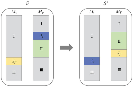
Step 2: Enforcing Light Job Monotonicity. Suppose that $J_j$ is a light job that is not assigned to the available machine $M_i$ with the smallest index, but is instead scheduled on a later machine $M_{i^{\prime }}$ with $i^{\prime }>i$. Let $J_{j^{\prime }}$ be the earliest subsequent job ($j^{\prime }>j$) that is assigned to machine $M_i$. We divide the job sequence into three consecutive phases: Phase I includes jobs scheduled before $J_j$; Phase II consists of jobs from $J_j$ to $J_{j^{\prime }}$; and Phase III includes jobs scheduled after $J_{j^{\prime }}$, as shown on the left side of Figure 1. We construct a new schedule ${\mathcal{S}}^{*}$ by swapping the assignments of $J_j$ and $J_{j^{\prime }}$, reassigning $J_j$ to machine $M_i$ and $J_{j^{\prime }}$ to machine $M_{i^{\prime }}$, as shown on the right side of Figure 1. Since the original schedule $\mathcal{S}$ satisfies job number monotonicity, the slot position of $J_{j^{\prime }}$ in ${\mathcal{S}}^{*}$ does not increase. Moreover, because $J_j$ is a light job with negligible cost, this reassignment does not increase the total energy cost. The updated schedule ${\mathcal{S}}^{*}$ continues to maintain job number monotonicity. Therefore, this correction process can be applied iteratively until light job monotonicity is fully achieved.

Figure 1. Correction of light job monotonicity by reassigning a light job to the smallest-indexed available machine.

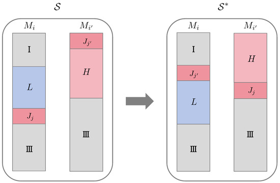
Step 3: Enforcing Heavy Job Monotonicity. Assume that the first violation of heavy job monotonicity occurs when a heavy job $J_j$ is assigned to machine $M_i$, despite the existence of an earlier heavy job $J_{j^{\prime }}$ ($j^{\prime }<j$) that was previously assigned to a later machine $M_{i^{\prime }}$ with $i^{\prime }>i$. In other words, $J_j$ is scheduled to a machine with a smaller index than a preceding heavy job, violating the required non-decreasing order of machine indices for heavy job assignments. We focus on this first violation, as depicted on the left side of Figure 2. Since machine $M_i$ was still available at the time $J_j$ was scheduled (i.e., $a_i(j-1)<n$), light job monotonicity ensures that no light jobs could have been assigned to $M_{i^{\prime }}$ before $J_j$. Therefore, all jobs on $M_{i^{\prime }}$ scheduled before $J_j$ must be heavy jobs, labeled as set $\mathcal{H}$ in the figure. Let $J_{j^{\prime }}$ be the earliest such heavy job on $M_{i^{\prime }}$.

Figure 2. Swap-based correction of heavy job monotonicity to ensure non-decreasing machine indices for earlier jobs.

Meanwhile, because $J_j$ represents the first violation of heavy job monotonicity, all jobs scheduled to $M_i$ between $J_{j^{\prime }}$ and $J_j$ must be light jobs. These are labeled as set $\mathcal{L}$ in Figure 2. The job sequence is thus divided into three phases: Phase I consists of all jobs prior to $J_{j^{\prime }}$; Phase II spans from $J_{j^{\prime }}$ to $J_j$, and includes both heavy jobs on $M_{i^{\prime }}$ (set $\mathcal{H}$) and light jobs on $M_i$ (set $\mathcal{L}$); and Phase III contains all jobs after $J_j$. To restore monotonicity, we construct a new schedule ${\mathcal{S}}^{*}$ by swapping the assignments of $J_j$ and $J_{j^{\prime }}$, reassigning $J_j$ to machine $M_{i^{\prime }}$ and $J_{j^{\prime }}$ to machine $M_i$, as illustrated on the right side of Figure 2. Since $M_i$ has only received light jobs between $J_{j^{\prime }}$ and $J_j$, and because light jobs incur negligible energy cost, this swap does not affect the overall cost contribution of the light jobs. Furthermore, the slot index of $J_{j^{\prime }}$ in ${\mathcal{S}}^{*}$ is no greater than in the original schedule $\mathcal{S}$, and the number of heavy jobs assigned to $M_{i^{\prime }}$ remains unchanged. As the slot cost function is fixed and strictly increasing, the total energy cost does not increase.

Importantly, the reassignment does not violate light job monotonicity, and the updated schedule ${\mathcal{S}}^{*}$ continues to satisfy job number monotonicity. Therefore, this correction procedure can be applied iteratively until all violations of heavy job monotonicity are eliminated.

Termination and Feasibility: Each of the above transformations resolves one violation without introducing new ones, and there is a finite number of jobs. Therefore, the process terminates in finite steps. The resulting schedule ${\mathcal{S}}^{*}$ is feasible, satisfies all three monotonicity conditions, and achieves

$$\mathrm{TotalCost}\left({\mathcal{S}}^{*}\right)\le \mathrm{TotalCost}\left(\mathcal{S}\right). \square$$

3.2. Constructing Monotonic Assignments via Heavy Job Distribution

A monotonic machine assignment can be completely specified by a vector of heavy job quotas $\{h_1,h_2,\dots ,h_m\}$, where $h_i$ denotes the number of heavy jobs assigned to machine $M_i$, and the total number of heavy jobs satisfies

$$\sum _{i=1}^m{h}_i=H,$$

(13)

with H denoting the total number of heavy jobs in the system.

Given a fixed job arrival sequence and a heavy job distribution vector, the monotonic machine assignment can be constructed by assigning each job dynamically based on its type, as outlined in Algorithm 1.

Assignment Rules.

• Heavy jobs: Assign each heavy job $J_j$ to the first available machine $M_i$ (smallest index) such that $h_i^{\mathrm{remaining}}>0$ and $a_i<n$;
• Light jobs: Assign each light job $J_j$ to the first machine $M_i$ (smallest index) with an available slot, i.e., $a_i(j-1)<n$.

Here, $h_i^{\mathrm{remaining}}$ is the number of heavy jobs remaining to be assigned to machine $M_i$, and $a_i$ tracks the number of total jobs (heavy or light) assigned to $M_i$ thus far.

Algorithm 1 Monotonic assignment construction from heavy quotas.

1: for each machine $M_i\in \mathcal{M}$ do 2:    Initialize $h_i^{\mathrm{remaining}}\leftarrow h_i$    {heavy jobs remaining for $M_i$} 3:    Initialize $a_i\leftarrow 0$    {current number of jobs assigned to $M_i$} 4: end for 5: for each job $J_j$ in arrival order do 6:    if $J_j$ is a heavy job then 7:      Find the smallest i such that $h_i^{\mathrm{remaining}}>0$ and $a_i<n$ 8:      Assign $J_j$ to $M_i$ 9:      Update $h_i^{\mathrm{remaining}}\leftarrow h_i^{\mathrm{remaining}}-1$, $a_i\leftarrow a_i+1$ 10:    else 11:      Find the smallest i such that $a_i<n$ 12:      Assign $J_j$ to $M_i$ 13:      Update $a_i\leftarrow a_i+1$ 14:    end if 15: end for

  Feasibility Condition: Not all heavy job vectors satisfying ${\sum }_{i=1}^m{h}_i=H$ correspond to feasible schedules. To ensure feasibility, each machine $M_i$ must always have sufficient capacity to accommodate its remaining heavy job quota at every stage of the sequential assignment. That is, the following constraint must be satisfied throughout the process:

$$n-a_i\ge h_i^{\mathrm{remaining}},\forall M_i\in \mathcal{M}.$$

(14)

We define ${\overline{h}}_i$ as the number of heavy jobs in the i-th block of the job sequence $\mathcal{J}$, given by

$${\overline{h}}_i=\sum _{j=(i-1)n+1}^{i·n}{t}_j.$$

(15)

Then, a heavy job allocation vector $\{h_1,h_2,\dots ,h_m\}$ is feasible if and only if

$$\sum _{k=1}^i{h}_k\le \sum _{k=1}^i{\overline{h}}_k,\mathrm{and}0\le h_i\le n\mathrm{for}\mathrm{all}i=1,2,\dots ,m.$$

(16)

3.3. Dynamic Programming for Optimal Monotonic Assignment

We present a dynamic programming algorithm to compute an optimal monotonic machine assignment, minimizing total energy cost under a fixed job arrival order and slot-based cost structure.

DP State Definition: Let DP[i][h] denote the minimum total cost of assigning the first i machines with exactly h heavy jobs scheduled in total.

  Transition Function: Let $g_i(k,h^{\prime })$ represent the minimum cost of assigning exactly k heavy jobs and $n-k$ light jobs to machine $M_i$, assuming that $h^{\prime }$ heavy jobs have already been scheduled across the first $i-1$ machines. Then, the recurrence is

$$\mathtt{DP}\left[i\right]\left[h\right]=\underset{0\le k\le min(n,h)}{min}\left\{\mathtt{DP}[i-1][h-k]+g_i(k,h-k)\right\},$$

(17)

with the base cases

$$\mathtt{DP}\left[0\right]\left[0\right]=0,\mathtt{DP}\left[0\right]\left[h\right]=\infty \mathrm{for}h>0.$$

The final solution is given by

$$\mathtt{DP}\left[m\right]\left[H\right],\mathrm{where}H=\sum _{j=1}^{nm}{t}_j\mathrm{is}\mathrm{the}\mathrm{total}\mathrm{number}\mathrm{of}\mathrm{heavy}\mathrm{jobs}.$$

  Feasibility Condition: If assigning k heavy jobs to machine $M_i$ is infeasible—e.g., there are insufficient remaining heavy jobs or too few available slots due to prior light jobs—then $g_i(k,h^{\prime })$ is set to $+\infty$ and excluded from the transition.

  Time Complexity: The total number of DP states is

$$\sum _{i=1}^m(i·n+1)=\mathcal{O}\left(n{m}^2\right).$$

Each state enumerates up to n values of k, and the corresponding $g_i(k,h^{\prime })$ values are retrieved in $\mathcal{O}\left(1\right)$ time via preprocessing. Hence, the total time complexity of the dynamic programming procedure is

$$\mathcal{O}\left(n\right)\mathrm{per}\mathrm{state}\times \mathcal{O}\left(n{m}^2\right)\mathrm{states}=\begin{array}{|c|}\hline \mathcal{O}\left(n^2{m}^2\right)\\ \hline\end{array}.$$

  Preprocessing of Transition Costs: Each $g_i(k,h^{\prime })$ value is computed by selecting the appropriate subsequence of jobs to be assigned to machine $M_i$, and calculating the total slot cost of the top-k heavy jobs within that segment. This preprocessing step is efficiently performed using a prefix sum or scan-based technique, as detailed in Algorithm 2. For any fixed machine index i and heavy job prefix count $h^{\prime }$, the full cost vector ${\left\{g_i(k,h^{\prime })\right\}}_{k=0}^n$ can be computed in $\mathcal{O}\left(n\right)$ time. Since there are at most $nm$ distinct values of $h^{\prime }$ (i.e., the number of ways to distribute heavy jobs across the first $i-1$ machines), and m choices of i, the total number of $(i,h^{\prime })$ pairs is $\mathcal{O}\left(n{m}^2\right)$. Therefore, the total time required to compute all $g_i(k,h^{\prime })$ values for all machines and heavy job prefix states is

$$\mathcal{O}\left(n\right)(\mathrm{per}\mathrm{pair})\times \mathcal{O}\left(n{m}^2\right)(\mathrm{number}\mathrm{of}\mathrm{pairs})=\begin{array}{|c|}\hline \mathcal{O}\left(n^2{m}^2\right)\\ \hline\end{array}.$$

Thus, the overall time complexity of the proposed algorithm—including both dynamic programming and preprocessing of all $g_i(k,h^{\prime })$ values—is

$$\begin{array}{|c|}\hline \mathcal{O}\left(n^2{m}^2\right)\\ \hline\end{array}.$$

Algorithm 2 ComputeAllGi: Preprocessing $g_i(k,h^{\prime })$ for machine $M_i$.

Require: job sequence $t[1\dots nm]$, machine index i, total number of heavy jobs scheduled so far: $h^{\prime }$ Ensure: Array $g[0\dots n]$, where $g\left[k\right]$ is the cost of assigning k heavy jobs to $M_i$ 1: Filter the job sequence to select the next n jobs assigned to $M_i$: Skip the first h heavy jobs, Skip the first $(i-1)n-h$ light jobs, Select the next n jobs to form the assignment block for $M_i$. 2: Let $\mathtt{heavy}\_\mathtt{pos}$ be the indices of heavy jobs in the selected n jobs. 3: for$k=0$ to n do 4:    if $i=m$$k\ne |\mathtt{heavy}\_\mathtt{pos}|$ then 5:      $g\left[k\right]\leftarrow \infty$    {Final machine must take remaining heavy jobs} 6:    else if $k>|\mathtt{heavy}\_\mathtt{pos}|$ then 7:      $g\left[k\right]\leftarrow \infty$          {Not enough heavy jobs available} 8:    else 9:      $g\left[k\right]\leftarrow {\sum }_{j=1}^{k}s[\mathtt{heavy}\_\mathtt{pos}\left[j\right]]$ 10:    end if 11: end for 12: returng

4. Misalignment Elimination Algorithm

In this section, we develop an iterative refinement algorithm that transforms an initial feasible assignment into an optimal monotonic one. Building on the structural properties of the assignment, we identify local inconsistencies—referred to as misaligned assignments—and propose a targeted adjustment strategy to eliminate them. The algorithm operates by incrementally resolving these misalignments, one at a time, while ensuring that feasibility is preserved and the total cost does not increase. Through repeated application of this refinement step, the algorithm progressively improves the assignment structure until all machines are properly aligned. We provide both the algorithmic procedure and a formal proof of its correctness and computational efficiency.

4.1. Misaligned Assignment

Definition 1 (Misaligned Assignment).

Given a monotonic machine assignment $\mathcal{S}$, we denote a misaligned assignment on adjacent machines $M_i$ and $M_{i+1}$ if the slot index of the last heavy job on $M_i$ is greater than or equal to that of the first light job on $M_{i+1}$. This implies a sub-optimal assignment of heavy and light jobs across adjacent machines, which may degrade scheduling efficiency. Formally, let the following hold:

• $p^{\mathcal{S}}\left(i\right)$ denotes the slot index of the last heavy job assigned to $M_i$ (with $p^{\mathcal{S}}\left(i\right)=0$ if no heavy job exists);
• $q^{\mathcal{S}}\left(i\right)$ denotes the slot index of the first light job assigned to $M_i$ (with $q^{\mathcal{S}}\left(i\right)=n+1$ if no light job exists).

• Then machines $M_i$ and $M_{i+1}$ are said to be misaligned if

  $$p^{\mathcal{S}}\left(i\right)\ge q^{\mathcal{S}}(i+1).$$
• For notational simplicity, we may omit the superscript $\mathcal{S}$ when the assignment context is clear.

Consider two consecutive machines $M_i$ and $M_{i+1}$ that exhibit a misaligned assignment. Let $J_j$ denote the last heavy job assigned to $M_i$, and $J_{j^{\prime }}$ denote the first light job assigned to $M_{i+1}$, as illustrated on the left side of Figure 3. To eliminate this misalignment, we construct a new assignment ${\mathcal{S}}^{*}$ by swapping these two jobs: $J_j$ is reassigned to $M_{i+1}$, and $J_{j^{\prime }}$ is reassigned to $M_i$, as shown on the right side of the Figure 3. Since the slot index of job $J_j$ on machine $M_i$ is no smaller than that of job $J_{j^{\prime }}$ on machine $M_{i+1}$ (i.e., $p^{\mathcal{S}}\left(i\right)\ge q^{\mathcal{S}}(i+1)$), the reassignment does not increase the total energy cost. Furthermore, the reassignment updates the number of heavy jobs as follows:

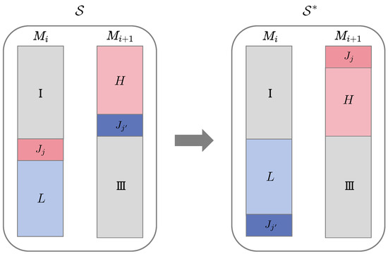
Figure 3. Elimination of a misaligned assignment by exchanging a heavy job with a light job between adjacent machines.

• Machine $M_i$: $h_i\to h_i-1$;
• Machine $M_{i+1}$: $h_{i+1}\to h_{i+1}+1$.

The swap affects only the slot configuration of machines $M_i$ and $M_{i+1}$. Specifically, the following properties hold in the updated assignment ${\mathcal{S}}^{*}$:

• $p^{{\mathcal{S}}^{*}}\left(i\right)<p^{\mathcal{S}}\left(i\right)$;
• $q^{{\mathcal{S}}^{*}}\left(i\right)\le q^{\mathcal{S}}\left(i\right)$;
• $p^{{\mathcal{S}}^{*}}(i+1)\ge p^{\mathcal{S}}(i+1)$;
• $q^{{\mathcal{S}}^{*}}(i+1)>q^{\mathcal{S}}(i+1)$.

These local updates imply that the misalignment condition $p^{\mathcal{S}}\left(i\right)\ge q^{\mathcal{S}}(i+1)$ may no longer hold in the updated assignment $\mathcal{S}*$, thereby resolving the inconsistency between machines $M_i$ and $M_{i+1}$. However, this swap may introduce new misalignments involving adjacent machine pairs, specifically $(i-1,i)$ or $(i+1,i+2)$. Nevertheless, each swap strictly improves the structural alignment by moving a heavy job forward along the machine sequence. Since there are at most $nm$ heavy jobs in total, and each job can traverse at most m machines (from $M_1$ to $M_m$ in the worst case), the total number of swaps is bounded by $\mathcal{O}(nm·m)=\mathcal{O}\left(n{m}^2\right)$.

4.2. Efficient Computation of Slot Positions

Let $\mathtt{light}\_\mathtt{prefix}\left[j\right]$ and $\mathtt{heavy}\_\mathtt{prefix}\left[j\right]$ denote the cumulative number of light and heavy jobs, respectively, among the first j jobs in the input sequence:

$$\mathtt{light}\_\mathtt{prefix}\left[j\right]=\sum _{\ell =1}^j{\mathbf{1}}_{\{t_{\ell }=0\}},\mathtt{heavy}\_\mathtt{prefix}\left[j\right]=\sum _{\ell =1}^j{\mathbf{1}}_{\{t_{\ell }=1\}}.$$

Let $x=h_i$ be the number of heavy jobs assigned to machine $M_i$, and let $y={\sum }_{k=1}^{i-1}{h}_k$ denote the total number of heavy jobs assigned to machines $M_1$ through $M_{i-1}$.

  (1) Computation of $p\left(i\right)$: The total number of heavy jobs assigned to the first i machines is $x+y$. The last heavy job assigned to machine $M_i$ corresponds to the $(x+y)$-th heavy job in the global sequence. Let j be the smallest index such that

$$\mathtt{heavy}\_\mathtt{prefix}\left[j\right]=x+y.$$

The number of light jobs among the first j jobs is $\mathtt{light}\_\mathtt{prefix}\left[j\right]$, and the number of light jobs assigned to machines $M_1$ through $M_{i-1}$ is $n(i-1)-y$. Let

$$\ell =\mathtt{light}\_\mathtt{prefix}\left[j\right]-\left(n(i-1)-y\right)$$

denote the number of light jobs already assigned to machine $M_i$ before job $J_j$. Then, the slot position of the last heavy job $J_j$ on $M_i$ is

$$p\left(i\right)=\left\{\begin{array}{cc}\ell +x,\hfill & \mathrm{if}\ell \ge 0\hfill \\ x,\hfill & \mathrm{if}\ell <0\hfill \end{array}\right.$$

  (2) Computation of $q\left(i\right)$: The number of light jobs assigned to machines $M_1$ through $M_{i-1}$ is $n(i-1)-y$. Hence, the first light job assigned to machine $M_i$ corresponds to the $\left(n\right(i-1)-y+1)$-th light job in the global sequence. Let j be the smallest index such that

$$\mathtt{light}\_\mathtt{prefix}\left[j\right]=n(i-1)-y+1.$$

The number of heavy jobs among the first j jobs is $\mathtt{heavy}\_\mathtt{prefix}\left[j\right]$, and the number of heavy jobs already assigned to machines $M_1$ through $M_{i-1}$ is y. Let

$$\ell =\mathtt{heavy}\_\mathtt{prefix}\left[j\right]-y$$

denote the number of heavy jobs already assigned to machine $M_i$ before job $J_j$. Then, the slot position of this first light job $J_j$ on $M_i$ is

$$q\left(i\right)=\left\{\begin{array}{cc}\ell +1,\hfill & \mathrm{if}\ell \le x\hfill \\ x+1,\hfill & \mathrm{if}\ell >x\hfill \end{array}\right.$$

  Both prefix arrays can be preprocessed in $\mathcal{O}\left(mn\right)$ time. By recording the first occurrence of each prefix value, the queries for $p\left(i\right)$ and $q\left(i\right)$ can be answered in constant time using hash maps or direct indexing. Consequently, both slot positions can be computed in $\mathcal{O}\left(1\right)$ time per query.

4.3. Misalignment Elimination Algorithm

We now present the complete iterative refinement procedure in Algorithm 3, which incrementally eliminates misaligned assignments until none remain, ultimately yielding an optimal monotonic assignment. The algorithm begins with the initial heavy job distribution ${\overline{h}}_1,{\overline{h}}_2,\dots ,{\overline{h}}_m$, computed directly from the input job sequence. It then maintains a dynamic misalignment set C, which stores the indices of all machines currently involved in misaligned assignments, based on the slot positions $p\left(i\right)$ and $q\left(i\right)$.

This reassignment strategy preserves feasibility at every step and ensures that the total assignment cost is non-increasing. Importantly, due to the monotonic behavior of $p\left(i\right)$ and $q\left(i\right)$ during each swap, the misalignment set C is only locally affected. Specifically, machine pairs that do not involve indices i or $i+1$ remain unaffected. This locality property guarantees that each iteration modifies only a small portion of the assignment and simplifies the update of C.

Algorithm 3 Misalignment elimination algorithm.

Require: Job types sequence $(t_1,t_2,\dots ,t_{mn})$, number of machines m, slot size n Ensure: Optimized heavy job counts $h_1,h_2,\dots ,h_m$ 1: Initialize misalignment set $C\leftarrow \varnothing$ 2: for each machine $i=1$ to m do 3:    Set $h_i\leftarrow {\sum }_{j=(i-1)·n+1}^{i·n}{t}_j$ {Initial heavy job count on machine i} 4:    Compute $p\left(i\right)$ and $q\left(i\right)$ 5:    if $p(i-1)\ge q\left(i\right)$ then 6:         $C\leftarrow C\cup \{i-1\}$ 7:    end if 8: end for 9: while $C\ne \varnothing$ do 10:    Select any $i\in C$ 11:    Update $h_i\leftarrow h_i-1$, $h_{i+1}\leftarrow h_{i+1}+1$ 12:    Update $p\left(i\right)$, $q\left(i\right)$, $p(i+1)$, $q(i+1)$ 13:    for each $k\in \{i-1,i,i+1\}$ such that $1\le k<m$ do 14:      if $p\left(k\right)\ge q(k+1)$ then 15:         $C\leftarrow C\cup \left\{k\right\}$ 16:      else 17:         $C\leftarrow C\setminus \left\{k\right\}$ 18:      end if 19:    end for 20: end while 21: return $h_1,\dots ,h_m$

Moreover, the slot positions $p\left(i\right)$ and $q\left(i\right)$ can be maintained and updated in constant time per iteration, i.e., $\mathcal{O}\left(1\right)$, as previously discussed. Since each iteration performs a single resolution step by relocating one heavy job between adjacent machines, and each heavy job can be moved across at most m machines, the total number of iterations is bounded by $\mathcal{O}\left(n{m}^2\right)$. As each iteration requires constant time, the overall time complexity of the algorithm is $\mathcal{O}\left(n{m}^2\right)$. The memory usage is $\mathcal{O}\left(nm\right)$.

We summarize the correctness and computational complexity of the proposed method in the following theorem.

Theorem 2.

The misalignment elimination algorithm computes an optimal monotonic assignment in $\mathcal{O}\left(n{m}^2\right)$ time.

Proof. 

This proof is primarily devoted to establishing the optimality of the output produced by the misalignment elimination algorithm. The time complexity of the method has already been analyzed earlier and is not the focus here. We denote by $\varphi \left(\mathcal{S}\right)$ the assignment produced by the misalignment elimination algorithm when starting from the initial assignment $\mathcal{S}$.

We first prove that the algorithm always converges to a unique assignment. Assume, for the sake of contradiction, that the algorithm terminates at two distinct monotonic assignment vectors, denoted by ${\mathcal{S}}^1$ and ${\mathcal{S}}^2$, such that ${\mathcal{S}}^1\ne {\mathcal{S}}^2$. Without loss of generality, let i be the smallest index such that ${\mathcal{S}}_i^1>{\mathcal{S}}_i^2$. Then there exists an intermediate assignment ${\mathcal{S}}^{\prime }$, which occurs during the execution of the algorithm that leads to ${\mathcal{S}}^2$, such that the partial sum up to index i satisfies

$$\sum _{k\le i}{\mathcal{S}}_k^{\prime }=\sum _{k\le i}{\mathcal{S}}_k^1,$$

and yet ${\mathcal{S}}^{\prime }$ contains a misalignment at index i, that is,

$$p^{{\mathcal{S}}^{\prime }}\left(i\right)\ge q^{{\mathcal{S}}^{\prime }}(i+1).$$

By the monotonicity of the assignment process, we have

$$p^{{\mathcal{S}}^1}\left(i\right)\ge p^{{\mathcal{S}}^{\prime }}\left(i\right)\ge q^{{\mathcal{S}}^{\prime }}(i+1)\ge q^{{\mathcal{S}}^1}(i+1),$$

which implies $p^{{\mathcal{S}}^1}\left(i\right)\ge q^{{\mathcal{S}}^1}(i+1)$, contradicting the assumption that ${\mathcal{S}}^1$ is misalignment-free. Therefore, the algorithm must converge to a unique final assignment.

Next, we show that the algorithm’s final assignment is optimal. Let ${\mathcal{S}}^{*}=(h_1^{*},h_2^{*},\dots ,h_m^{*})$ denote the optimal initial assignment, i.e., the one that minimizes total cost among all monotonic assignments. Then $\varphi \left({\mathcal{S}}^{*}\right)=(x_1^{*},x_2^{*},\dots ,x_m^{*})$ is the corresponding optimal misalignment-free assignment produced by the algorithm $\varphi$. Let the assignment generated from the natural initial input $({\overline{h}}_1,{\overline{h}}_2,\dots ,{\overline{h}}_m)$ be $\varphi ({\overline{h}}_1,{\overline{h}}_2,\dots ,{\overline{h}}_m)=(x_1,x_2,\dots ,x_m)$.

We prove by induction on m that $\varphi ({\overline{h}}_1,{\overline{h}}_2,\dots ,{\overline{h}}_m)=\varphi \left({\mathcal{S}}^{*}\right)$. That is, we show that the final assignments match:

$$(x_1,x_2,\dots ,x_m)=(x_1^{*},x_2^{*},\dots ,x_m^{*}).$$

Base case: When $m=1$, the result holds trivially since all heavy jobs must be assigned to the single machine.

Inductive step: Assume the claim holds for $m-1$. For the case of m machines, we compare the first coordinate of the final assignment.

Suppose $x_1<x_1^{*}$. Consider the modified input

$$(x_1^{*},{\overline{h}}_2+({\overline{h}}_1-x_1^{*}),{\overline{h}}_3,\dots ,{\overline{h}}_m),$$

which preserves the total number of heavy jobs. By the monotonicity of $\varphi$, we obtain

$$\varphi ({\overline{h}}_1,{\overline{h}}_2,\dots ,{\overline{h}}_m)=\varphi (x_1^{*},{\overline{h}}_2+({\overline{h}}_1-x_1^{*}),{\overline{h}}_3,\dots ,{\overline{h}}_m).$$

Now, by the induction hypothesis, we know that

$$\varphi ({\overline{h}}_2+({\overline{h}}_1-x_1^{*}),{\overline{h}}_3,\dots ,{\overline{h}}_m)=(x_2^{*},\dots ,x_m^{*}),$$

so the entire assignment equals $(x_1^{*},x_2^{*},\dots ,x_m^{*})$, contradicting the assumption $x_1<x_1^{*}$.

Now suppose $x_1>x_1^{*}$. Because the algorithm $\varphi$ moves heavy jobs forward to eliminate misalignments, once the assignment becomes misalignment-free, any further movement of heavy jobs would violate the alignment constraint and increase the total cost due to the monotonic increase in slot costs. Thus, no additional improvement is possible beyond the optimal misalignment-free configuration.

Applying this logic repeatedly, we obtain

$$\begin{array}{cc}\hfill \mathrm{TotalCost}(x_1,x_2,\dots ,x_m)& <\mathrm{TotalCost}\left(\varphi (x_1-1,x_2+1,x_3,\dots ,x_m)\right)\hfill \\ \hfill & <\mathrm{TotalCost}\left(\varphi (x_1-2,x_2+2,x_3,\dots ,x_m)\right)\hfill \\ \hfill & ⋮\hfill \\ \hfill & <\mathrm{TotalCost}\left(\varphi (x_1^{*},x_2+x_1-x_1^{*},x_3,\dots ,x_m)\right)\hfill \\ \hfill & =\mathrm{TotalCost}(x_1^{*},x_2^{*},\dots ,x_m^{*}),\hfill \end{array}$$

where the last equality follows from the induction hypothesis. This contradicts the optimality of the corresponding optimal misalignment-free assignment produced by the algorithm $\varphi$.

Therefore, we must have $x_1=x_1^{*}$. By the induction hypothesis again, the assignments on the remaining $m-1$ machines also match. Thus, the entire final assignment produced by the algorithm matches the optimal one:

$$(x_1,x_2,\dots ,x_m)=(x_1^{*},x_2^{*},\dots ,x_m^{*}).$$

   □

4.4. Experimental Evaluation

To evaluate the computational efficiency of the proposed misalignment elimination algorithm, a comprehensive runtime comparison was conducted against a baseline dynamic programming approach. The comparison focuses on two dimensions: the number of machines m, and the ratio of heavy jobs $\rho =H/N$, under realistic scheduling configurations.

Implementation Details: All algorithms were implemented in C++17 and compiled with g++ using the -O2 optimization flag. Experiments were executed on a Linux machine with an Intel i7-12700H CPU and 32 GB RAM. High-precision timing was measured using std::chrono. For each data point, 100 random instances were generated with fixed parameters, and the average runtime was recorded to reduce variance.

Each test case consists of $N=m\times n$ jobs, with exactly $H=\rho N$ heavy jobs, randomly mixed with $N-H$ light jobs. The binary job sequence is randomly shuffled using std::shuffle to ensure unbiased sampling.

Scaling with Machine Number: The number of machines $m\in \{10,20,\dots ,90\}$ was varied while keeping the slot number fixed at $n=5$ and the heavy job ratio constant at $\rho =0.3$. As illustrated in the left panel of Figure 4, the runtime of the dynamic programming method increases rapidly with m, exhibiting a clear quadratic trend. This is consistent with its theoretical complexity of $\mathcal{O}\left(n^2{m}^2\right)$, where both the number of machines and the slot count contribute multiplicatively to the computational cost. Since n is fixed in this experiment, the observed runtime growth reflects the $m^2$ term in the complexity, confirming that the method becomes substantially more expensive as the number of machines increases.

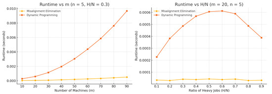
Figure 4. Comparison of misalignment elimination and dynamic programming runtime under varying machine numbers and heavy job ratios.

In contrast, the misalignment elimination method achieves significantly faster runtime and better scalability. By targeting only local conflicts and incrementally refining job assignments, it avoids the combinatorial overhead of global enumeration. The observed runtime follows a near-quadratic pattern, consistent with its theoretical bound of $\mathcal{O}\left(n{m}^2\right)$, yet with substantially smaller constant factors. This efficiency enables it to handle large-scale instances with minimal delay, demonstrating clear practical advantages over dynamic programming.

Scaling with Heavy Job Ratio: With machine and slot counts fixed at $m=20$ and $n=5$, the heavy job ratio $\rho \in [0.1,0.9]$ was varied. The right panel of Figure 4 shows that dynamic programming runtime increases with $\rho$, peaking around $\rho =0.6$ due to a denser and more complex state space. Slight reductions beyond this point are attributed to more uniform job types reducing branching complexity.

Meanwhile, misalignment elimination remains consistently fast across all $\rho$, showing only minor variation. This robustness arises from its conflict-driven logic, which depends primarily on local slot-level constraints rather than the global distribution of job types.

Across both scaling dimensions, misalignment elimination demonstrates significantly better runtime performance than dynamic programming. It achieves reliable low-latency execution consistent with the $\mathcal{O}\left(n{m}^2\right)$ bound, making it more suitable for large-scale or real-time scheduling scenarios where computational efficiency is critical.

5. Conclusions

This paper investigates an energy-aware scheduling problem in which a fixed sequence of heterogeneous jobs must be assigned to multiple identical machines with monotonically increasing slot costs. A key observation is that the contribution of light jobs remains invariant across all feasible assignments. This enables the problem to be reformulated as minimizing the cumulative cost associated with heavy job placements. To address the cost asymmetry under structural constraints, we propose the concept of monotonic machine assignment, which imposes index-based rules to guide job placement and restore regularity. This structure-aware reformulation narrows the solution space without sacrificing optimality, thereby facilitating efficient algorithmic design.

Based on this framework, we develop two optimal algorithms: a dynamic programming method with time complexity $O\left(n^2{m}^2\right)$ and a more scalable misalignment elimination algorithm that achieves global optimality in $O\left(n{m}^2\right)$ time. Although the machines are structurally symmetric, inherent asymmetry in job costs and arrival order can lead to imbalanced naive assignments. In contrast, optimal solutions restore regularity through structured job allocation. Beyond algorithmic efficiency, the monotonic assignment model offers structural insight into how order-based constraints can be exploited to reduce complexity in asymmetric scheduling environments. This contributes to the broader literature on structure-aware optimization and highlights the role of latent regularities in enabling efficient scheduling under combinatorial constraints. Moreover, the simplicity and modularity of the proposed algorithms make them suitable for deployment in decentralized controllers, energy-sensitive embedded processors, and edge computing environments with real-time constraints.

While our algorithms are designed under a fixed job sequence and deterministic slot costs, this structural assumption reflects many real-world systems such as embedded controllers, pipelined compute chains, and energy-aware edge processors. In such environments, jobs typically arrive in a fixed order due to sensing or control dependencies, and energy or delay costs increase with position as a result of thermal buildup or battery degradation. Compared to heuristic or learning-based scheduling strategies, our model-driven approach provides structural transparency and provable optimality, without relying on extensive parameter tuning or large training datasets. Future research may explore online extensions or hybrid models that integrate structure-aware optimization with adaptive learning mechanisms. In addition, further directions include handling dynamically arriving jobs, accommodating heterogeneous machine architectures, and formulating multi-objective strategies that balance trade-offs between energy efficiency, latency, and fairness. It would also be valuable to investigate learning-based scheduling frameworks that adapt to workload patterns over time, as well as stochastic models that incorporate uncertainty in job characteristics and energy estimation.

References

- Gelenbe, E.; Caseau, Y. The impact of information technology on energy consumption and carbon emissions. Ubiquity 2015, 2015, 1–15. [Google Scholar] [CrossRef]
- Freitag, C.; Berners-Lee, M.; Widdicks, K.; Knowles, B.; Blair, G.; Friday, A. The climate impact of ICT: A review of estimates, trends and regulations. arXiv 2021, arXiv:2102.02622. [Google Scholar]
- Venu, G.; Vijayanand, K. Task scheduling in cloud computing: A survey. Int. J. Res. Appl. Sci. Eng. Technol. (IJRASET) 2020, 8, 2258–2266. [Google Scholar] [CrossRef]
- Ding, L.; Guan, Z.; Luo, D.; Rauf, M.; Fang, W. An adaptive search algorithm for multiplicity dynamic flexible job shop scheduling with new order arrivals. Symmetry 2024, 16, 641. [Google Scholar] [CrossRef]
- Mei, X.; Wang, Q.; Chu, X.; Liu, H.; Leung, Y.W.; Li, Z. Energy-aware task scheduling with deadline constraint in DVFS-enabled heterogeneous clusters. arXiv 2021, arXiv:2104.00486. [Google Scholar]
- Sharifi, M.; Taghipour, S. Optimal production and maintenance scheduling for a degrading multi-failure modes single-machine production environment. Appl. Soft Comput. 2021, 106, 107312. [Google Scholar] [CrossRef]
- Chen, N.; Chen, Y.; Yi, W.; Pei, Z. A novel DQN-based hybrid algorithm for integrated scheduling and machine maintenance in dynamic flexible job shops. IET Collab. Intell. Manuf. 2025, 7, e70028. [Google Scholar] [CrossRef]
- Kocot, B.; Czarnul, P.; Proficz, J. Energy-aware scheduling for high-performance computing systems: A survey. Energies 2023, 16, 890. [Google Scholar] [CrossRef]
- Yao, F.; Demers, A.; Shenker, S. A scheduling model for reduced CPU energy. In Proceedings of the IEEE 36th Annual Foundations of Computer Science, Milwaukee, WI, USA, 23–25 October 1995; pp. 374–382. [Google Scholar]
- Ben Alla, S.; Ben Alla, H.; Touhafi, A.; Ezzati, A. An efficient energy-aware tasks scheduling with deadline-constrained in cloud computing. Computers 2019, 8, 46. [Google Scholar] [CrossRef]
- Jiang, F.; Xia, Y.; Yan, L.; Liu, W.; Zhang, X.; Li, H.; Peng, J. Battery-aware workflow scheduling for portable heterogeneous computing. IEEE Trans. Sustain. Comput. 2024, 9, 677–694. [Google Scholar] [CrossRef]
- Albers, S. Energy-efficient algorithms. Commun. ACM 2010, 53, 86–96. [Google Scholar] [CrossRef]
- Mosheiov, G. Scheduling jobs under simple linear deterioration. Comput. Oper. Res. 1994, 21, 653–659. [Google Scholar] [CrossRef]
- Boddy, M.; Dean, T.L. Solving Time-Dependent Planning Problems; Brown University, Department of Computer Science: Providence, RI, USA, 1989. [Google Scholar]
- Ho, K.I.; Leung, J.Y.; Wei, W. Complexity of scheduling tasks with time-dependent execution times. Inf. Process. Lett. 1993, 48, 315–320. [Google Scholar] [CrossRef]
- Etgar, R.; Shtub, A.; LeBlanc, L.J. Scheduling projects to maximize net present value—The case of time-dependent, contingent cash flows. Eur. J. Oper. Res. 1997, 96, 90–96. [Google Scholar] [CrossRef]
- Ng, C.T.; Cheng, T.E.; Bachman, A.; Janiak, A. Three scheduling problems with deteriorating jobs to minimize the total completion time. Inf. Process. Lett. 2002, 81, 327–333. [Google Scholar] [CrossRef]
- Wang, Z.; Goudarzi, M.; Gong, M.; Buyya, R. Deep reinforcement learning-based scheduling for optimizing system load and response time in edge and fog computing environments. arXiv 2023, arXiv:2309.07407. [Google Scholar] [CrossRef]
- Hou, H.; Agos Jawaddi, S.N.; Ismail, A. Energy efficient task scheduling based on deep reinforcement learning in cloud environment: A specialized review. Future Gener. Comput. Syst. 2024, 151, 214–231. [Google Scholar] [CrossRef]
- López, M.; Stafford, E.; Bosque, J.L. Intelligent energy pairing scheduler (InEPS) for heterogeneous HPC clusters. J. Supercomput. 2025, 81, 427. [Google Scholar] [CrossRef]
- Mokhtari, M.; Mohamadi, P.H.A.; Aernouts, M.; Singh, R.K.; Vanderborght, B.; Weyn, M.; Famaey, J. Energy-aware multi-robot task scheduling using meta-heuristic optimization methods for ambiently-powered robot swarms. Robot. Auton. Syst. 2025, 186, 104898. [Google Scholar] [CrossRef]
- Mahmood, A.; Khan, S.A.; Albalooshi, F.; Awwad, N. Energy-aware real-time task scheduling in multiprocessor systems using a hybrid genetic algorithm. Electronics 2017, 6, 40. [Google Scholar] [CrossRef]
- Khaitan, S.K.; McCalley, J.D. Design techniques and applications of cyberphysical systems: A survey. IEEE Syst. J. 2015, 9, 350–365. [Google Scholar] [CrossRef]
- Esmaili, A.; Pedram, M. Energy-aware scheduling of jobs in heterogeneous cluster systems using deep reinforcement learning. In Proceedings of the 2020 21st International Symposium on Quality Electronic Design (ISQED), Santa Clara, CA, USA, 25–26 March 2020; pp. 426–431. [Google Scholar]
- Zhang, Y.W.; Chen, R.K. A survey of energy-aware scheduling in mixed-criticality systems. J. Syst. Archit. 2022, 127, 102524. [Google Scholar] [CrossRef]
- Kulkarni, J.; Munagala, K. Algorithms for cost-aware scheduling. In Proceedings of the International Workshop on Approximation and Online Algorithms, Ljubljana, Slovenia, 13–14 September 2012; Springer: Berlin/Heidelberg, Germany, 2012; pp. 201–214. [Google Scholar]
- Im, S.; Kulkarni, J.; Munagala, K. Competitive algorithms from competitive equilibria: Non-clairvoyant scheduling under polyhedral constraints. J. ACM 2017, 65, 1–33. [Google Scholar] [CrossRef]
- Chen, L.; Megow, N.; Rischke, R.; Stougie, L.; Verschae, J. Optimal algorithms and a PTAS for cost-aware scheduling. In Proceedings of the International Symposium on Mathematical Foundations of Computer Science, Milan, Italy, 24–28 August 2015; Springer: Berlin/Heidelberg, Germany, 2015; pp. 211–222. [Google Scholar]
- Epstein, L.; Levin, A.; Marchetti-Spaccamela, A.; Megow, N.; Mestre, J.; Skutella, M.; Stougie, L. Universal sequencing on a single machine. In Proceedings of the Integer Programming and Combinatorial Optimization, Lausanne, Switzerland, 9–11 June 2010; Springer: Berlin/Heidelberg, Germany, 2010; pp. 230–243. [Google Scholar]
- Burkard, R.E.; Rudolf, R.; Woeginger, G.J. Three-dimensional axial assignment problems with decomposable cost coefficients. Discret. Appl. Math. 1996, 65, 123–139. [Google Scholar] [CrossRef]
- Caseau, Y.; Laburthe, F. Solving various weighted matching problems with constraints. In Proceedings of the Principles and Practice of Constraint Programming-CP97, Linz, Austria, 29 October–1 November 1997; Smolka, G., Ed.; Springer: Berlin/Heidelberg, Germany, 1997; pp. 17–31. [Google Scholar]
- Chuzhoy, J.; Guha, S.; Khanna, S.; Naor, J.S. Machine minimization for scheduling jobs with interval constraints. In Proceedings of the 45th annual IEEE Symposium on Foundations of Computer Science, Rome, Italy, 17–19 October 2004; pp. 81–90. [Google Scholar]
- Im, S.; Li, S.; Moseley, B.; Torng, E. A dynamic programming framework for non-preemptive scheduling problems on multiple machines. In Proceedings of the Twenty-sixth Annual ACM-SIAM Symposium on Discrete Algorithms. SIAM, San Diego, CA, USA, 4–6 January 2015; pp. 1070–1086. [Google Scholar]
- Bansal, N.; Pruhs, K. The geometry of scheduling. SIAM J. Comput. 2014, 43, 1684–1698. [Google Scholar] [CrossRef]
- Wang, X.; Cao, J.; Buyya, R. Adaptive cloud bundle provisioning and multi-workflow scheduling via coalition reinforcement learning. IEEE Trans. Comput. 2022, 72, 1041–1054. [Google Scholar] [CrossRef]
- Chandrasiri, S.; Meedeniya, D. Energy-efficient dynamic workflow scheduling in cloud environments using deep learning. Sensors 2025, 25, 1428. [Google Scholar] [CrossRef]
- Hussain, M.; Wei, L.F.; Lakhan, A.; Wali, S.; Ali, S.; Hussain, A. Energy and performance-efficient task scheduling in heterogeneous virtualized cloud computing. Sustain. Comput. Inform. Syst. 2021, 30, 100517. [Google Scholar] [CrossRef]
- Grami, M. An energy-aware scheduling of dynamic workflows using big data similarity statistical analysis in cloud computing. J. Supercomput. 2022, 78, 4261–4289. [Google Scholar] [CrossRef]
- Brännvall, R.; Stark, T.; Gustafsson, J.; Eriksson, M.; Summers, J. Cost optimization for the edge-cloud continuum by energy-aware workload placement. In Proceedings of the Companion Proceedings of the 14th ACM International Conference on Future Energy Systems, New York, NY, USA, 20–23 June 2023; e-Energy ’23 Companion. pp. 79–84. [Google Scholar]
Disclaimer/Publisher’s Note: The statements, opinions and data contained in all publications are solely those of the individual author(s) and contributor(s) and not of MDPI and/or the editor(s). MDPI and/or the editor(s) disclaim responsibility for any injury to people or property resulting from any ideas, methods, instructions or products referred to in the content. |
© 2025 by the authors. Licensee MDPI, Basel, Switzerland. This article is an open access article distributed under the terms and conditions of the Creative Commons Attribution (CC BY) license (https://creativecommons.org/licenses/by/4.0/).