Composite Anti-Disturbance Static Output Control of Networked Nonlinear Markov Jump Systems with General Transition Probabilities Under Deception Attacks

Abstract

This paper studies the composite anti-disturbance static output feedback control problem of networked nonlinear Markov jump systems with general transition probabilities subject to multiple disturbances and deception attacks. The transition probabilities cover the known, uncertain with known bounds, and unknown cases. The unmatched disturbance and deception attacks are attenuated by the static output controller, while the matched disturbance is observed and compensated by the disturbance observer. Then, a composite anti-disturbance static output controller, including a linear part and a nonlinear part, is constructed to satisfy the stochastic $H_{\infty }$ stability. By using the Finsler lemma, sufficient conditions formed as symmetric linear matrix inequalities are derived to design the gains of disturbance observer and the output feedback controller. Finally, some simulations are given to illustrate the feasibility of the developed strategy.

1. Problem Statement and Preliminaries

As one type of representative stochastic systems, Markov jump systems (MJSs) have gained more and more attention and interest for their widespread applications in practical areas, such as networked systems, chemical processes, and manufacturing systems [1]. Regarding this system, fruitful works about stability and stabilization [2,3], sliding mode control [4,5], and event-triggered control [6,7] have been reported. These works always need a common hypothesis whereby the transition probabilities (TPs) are known completely. However, this is hard to realize due to measurement cost and error, and environment conditions, which limit its engineering applications. For example, in practical Markov jump power systems, TPs between normal and fault modes may be bounded using statistical fault rates due to unpredictable disturbances. Furthermore, for networked MJSs, communication delays and packet dropouts may cause abrupt mode changes with unknown TPs. Considering the TPs with known bounds, Ref. [8] studied the stability and stabilization issues for linear MJSs. Ref. [9] investigated the stabilization problem of linear MJSs with completely known and completely unknown TPs. In [10], a general case of TPs with known, uncertain, and unknown TPs was handled for the $H_{\infty }$ filtering problem of MJSs. Recently, with the development of the network technique, networked MJSs have become an interesting topic due to their features of low cost and high flexibility [11,12]. With the introduction of communication networks, the risk of communicated data being attacked by hackers increases dramatically, which could further cause system performance degradation and instability [13,14]. It is noted that the above outcomes are mostly based on the secure data transmissions of wired/wireless communication channel, while the cyber-attacks have been ignored.

On the other hand, it is known that disturbances caused by measurement noises and environment changes could degrade the system performance and even its stability. As an effective anti-disturbance control scheme, the disturbance-observer-based control (DOBC) has been investigated to compensate the degraded control performance caused by disturbances. Based on this scheme, many theoretical results can be found in [15,16,17,18], which are also applied in unmanned aerial vehicles [19], power systems [20], motor control systems [21], and so on. There are two main steps of the DOBC scheme. The first step is to obtain the estimation of the disturbance by constructing an observer. The second step is to design the linear control laws to satisfy the desired performance and add the estimated disturbance obtained by the observer into the control input to compensate the real disturbance. However, the simulation results in [15] show that if the disturbance contains norm-bounded terms, the DOBC scheme is infeasible for a class of nonlinear systems. To control the systems with multiple disturbances, composite control laws constituting DOBC and another control strategy have been addressed, for instance, robust control [22,23], and sliding mode control [24,25]. It is noted that most the above works are based on the full system state. However, the full state is difficult to obtain in real systems due to constraints of measurement costs and devices. As a result, Ref. [26] addressed the DOB output feedback control of the nonlinear MJSs. In their work, TPs were assumed to be known completely and a structure constraint was imposed on the Lyapunov variable. In addition, the dynamic output controller was designed in [26] to deal with the full state unavailable case, which is more complex and difficult than static output feedback control. In networked nonlinear MJSs, the matched disturbances induced by environment noises and changes of control channel, and the unmatched disturbances caused by parametric uncertainties or nonlinear dynamics, are usually unavoidable. In addition, due to the introduction of communication networks, the transmitted signals are highly likely to be attacked by adversaries. These factors make the control problems more complex, and some challenges are given below. First, the DOB compensation scheme for handling matched disturbance is based on measured output, which introduces some nonlinear terms raised from the disturbance observer gains and Lyapunov matrices. Second, the static output $H_{\infty }$ controller for dealing with mismatched disturbance and deception attacks is difficult to design due to the randomness of attacks and nonlinearity caused by controller gains and Lyapunov matrices. Third, the combination of the above two challenges and the nonlinearities resulting from general TPs of networked nonlinear MJSs further increases the challenge of solving the composite anti-disturbance static output control problem.

Inspired by the above observations, we investigate the composite anti-disturbance static output control of networked nonlinear MJSs with general TPs and deception attacks. First, a general case of TPs with known, uncertain with known bounds, and unknown parameters is considered. Second, a composite anti-disturbance static output controller is constructed to cope with the multiple disturbances. Specifically, the mismatched disturbance is attenuated by a static output controller and the matched disturbance is observed and mitigated by a disturbance observer. Third, the deception attacks on the control signal are modeled via a stochastic Bernoulli variable. Resorting to the Finsler lemma, the coupling among Lyapunov variable matrices and controller gains is removed by introducing new slack variables, and the diagonal structure constraint imposed on Lyapunov variable matrices in existing results [23,26] is not required any more. Meanwhile, this lemma can eliminate the nonlinearities caused by static output controller gains and slack variables. Compared to existing composite anti-disturbance control methods with completely known TPs [23,26], the unknown TPs are treated based on TP property and the proposed static output feedback controller. Moreover, it is easier to implement than the dynamic output controller in [26]. The control synthesis conditions are formed by linear matrix inequalities (LMIs), where matrix symmetry plays a critical role. The Lyapunov matrices and LMIs derived in the sufficient conditions inherently rely on symmetric properties to ensure stochastic $H_{\infty }$ stability, reflecting the mathematical symmetry in control system designs. Finally, a numerical example shows the validity of the proposed method.

• Notation: The symmetric elements in a matrix are represented by ∗. $He\left(X\right)$ means the operation of adding the matrix X and its transpose together. $\mathcal{E}\left\{x\right\}$ is the mathematical expectation of x. ${\mathcal{B}}^{\perp }$ denotes the null space matrix of $\mathcal{B}$.

Consider the following networked nonlinear MJSs:

$$\begin{array}{c}\hfill \left\{\begin{array}{c}\dot{x}\left(t\right)=A\left(r_t\right)x\left(t\right)+F\left(r_t\right)f(x\left(t\right),t)+G\left(r_t\right)[u\left(t\right)+d_1\left(t\right)]+H\left(r_t\right)d_2\left(t\right)]\hfill \\ z\left(t\right)=C_1\left(r_t\right)x\left(t\right)\hfill \\ y\left(t\right)=C\left(r_t\right)x\left(t\right)\hfill \end{array}\right.,\end{array}$$

(1)

where $x\left(t\right)\in {\mathbb{R}}^n$, $f(x\left(t\right),t)\in {\mathbb{R}}^p$, $u\left(t\right)\in {\mathbb{R}}^m$, $z\left(t\right)\in {\mathbb{R}}^q$, and $y\left(t\right)\in {\mathbb{R}}^p$ represent system state, nonlinear vector function, control input, performance output, and measured output, respectively. The disturbance $d_1\left(t\right)\in {\mathbb{R}}^m$, given in Assumption 1, can be used to describe the constant or harmonic noises. Another disturbance $d_2\left(t\right)\in {\mathbb{R}}^q$ belonging to ${\mathcal{L}}_2[0,\infty )$ can represent an arbitrary signal. $r_t\in \mathcal{I}=\{1,2,\dots ,s\}$ is a Markov process and simplified as i. The TPs are shown as follows:

$$Pr\{r_{t+h}=j|r_t=i\}=\left\{\begin{array}{cc}\hfill {\pi }_{ij}h+o\left(h\right),& i\ne j\hfill \\ \hfill 1+{\pi }_{ii}h+o\left(h\right),& i=j\hfill \end{array}\right.,$$

(2)

where $h>0$, ${\pi }_{ij}⩾0$ for $i\ne j$ and ${\pi }_{ii}=-{\displaystyle \sum _{j=1,j\ne i}^s}{\pi }_{ij}$ for each mode i, ${\displaystyle \underset{h\to 0}{lim}}o\left(h\right)/h=0$.

To deal with the difficulty of obtaining the complete TPs in practical systems, this paper considers the TPs with known, uncertain, and unknown cases. To see them clearly, we give a TP matrix ∏ with three modes as follows:

$$\prod =\left[\begin{array}{ccc}{\pi }_{11}& {\pi }_{12}& {\pi }_{13}\\ ?& ?& {\pi }_{23}+{\Delta }_{23}\\ {\pi }_{31}& {\pi }_{32}& {\pi }_{33}\end{array}\right],$$

(3)

where the known, uncertain, and unknown parameters are denoted by ${\pi }_{ij}$, ${\Delta }_{ij}\in [-{ϵ}_{ij}{ϵ}_{ij}]$, and “?”, respectively. For the convenience of derivation, all TPs are formulated via ${\widehat{\pi }}_{ij}$, which can be divided into the known (uncertain) and completely unknown cases:

$$\begin{array}{ccc}\hfill {\mathcal{I}}_k^i& =& \{j:{\widehat{\pi }}_{ij}denotesknownoruncertain\};\hfill \\ \hfill {\mathcal{I}}_{uk}^i& =& \{j:{\widehat{\pi }}_{ij}denotesunknown\}.\hfill \end{array}$$

Remark 1. 

It is noted that if all TPs are entirely unknown, stability analysis conditions and controller design conditions cannot be obtained by the TP-based method in this work. Then, the mode-dependent composite controller will become infeasible. Under this case, only TP-independent stability analysis and control design methods can be applied to stabilize the system.

Assumption 1 

([23]). The formulation of the disturbance $d_1\left(t\right)$ is given as follows:

$$\begin{array}{c}\hfill \left\{\begin{array}{c}\dot{\omega }\left(t\right)=W_i\omega \left(t\right)+M_i{d}_3\left(t\right)\hfill \\ d_1\left(t\right)=V_i\omega \left(t\right)\hfill \end{array}\right.,\end{array}$$

(4)

in which $W_i\in {\mathbb{R}}^{r\times r}$, $M_i\in {\mathbb{R}}^{r\times l}$, and $V_i\in {\mathbb{R}}^{m\times r}$ denote the constant matrices. $d_3\left(t\right)\in {\mathbb{R}}^l$ means the disturbance induced by the exogenous perturbations and uncertainties, which also satisfies ${\mathcal{L}}_2[0,\infty )$.

In order to compensate the effect of the disturbance $d_1\left(t\right)$ on control performance, the following disturbance observer model based on system output $y\left(t\right)$ is adopted to estimate $d_1\left(t\right)$:

$$\begin{array}{c}\hfill \left\{\begin{array}{c}{\widehat{d}}_1\left(t\right)=V_i\widehat{\omega }\left(t\right)\hfill \\ \widehat{\omega }\left(t\right)=v\left(t\right)-L_{i}y\left(t\right)\hfill \\ \dot{v}\left(t\right)=(W_i+L_i{C}_i{G}_i{V}_i)(v\left(t\right)-L_{i}y\left(t\right))+L_i{C}_i{G}_{i}u\left(t\right)\hfill \end{array}\right.,\end{array}$$

(5)

where $v\left(t\right)$ means observer state, $\widehat{\omega }\left(t\right)$ and ${\widehat{d}}_1\left(t\right)$ are the estimations of $\omega \left(t\right)$ and $d_1\left(t\right)$, and $L_i$ denotes the observer gain.

When the control signal is transmitted over the communication network, it is vulnerable to being attacked by external adversaries. Then, by using the measured output $y\left(t\right)$ and the estimated disturbance ${\widehat{d}}_1\left(t\right)$, the composite anti-disturbance static output controller is constructed as follows:

$$\begin{array}{c}\hfill u\left(t\right)=K_{i}y\left(t\right)-{\widehat{d}}_1\left(t\right)+\beta \left(t\right)\theta \left(t\right),\end{array}$$

(6)

in which $K_i$ means the controller matrix, $\theta \left(t\right)$ is the deception attack to change the control signal and satisfies

$$\begin{array}{c}\hfill {\parallel \theta \left(t\right)\parallel }_2\le {\parallel \mathsf{\Theta }x\left(t\right)\parallel }_2,\end{array}$$

(7)

with a constant known matrix $\mathsf{\Theta }$ representing the upper bound of attack function $\theta \left(t\right)$, and $\beta \left(t\right)$ is a random Bernoulli variable represents the attack happening or not. Specifically, $\beta \left(t\right)=1$ and $\beta \left(t\right)=0$ denote that the control signal is attacked and not attacked, respectively. Therefore, the occurrence probability of deception attacks is $\mathcal{E}\left\{\beta \left(t\right)\right\}={\beta }_1$.

Remark 2. 

Without considering the estimated disturbance ${\widehat{d}}_1\left(t\right)$ and deception attack $\theta \left(t\right)$, the composite anti-disturbance static output controller (6) reduces to

$$\begin{array}{c}\hfill u\left(t\right)=K_{i}y\left(t\right),\end{array}$$

(8)

which is the standard static output controller.

By combining (1), (4), (5), and (6), the augmented system is established as follows:

$$\begin{array}{c}\hfill \left\{\begin{array}{c}\dot{\xi }\left(t\right)={\overline{A}}_i\xi \left(t\right)+{\overline{F}}_{i}f(\xi \left(t\right),t)+{\overline{H}}_{i}d\left(t\right)+\beta \left(t\right){\overline{G}}_{i}g\left(t\right)\hfill \\ z\left(t\right)=C_{1i}x\left(t\right)+C_{2i}{e}_{\omega }\left(t\right)\triangleq {\overline{C}}_i\xi \left(t\right)\hfill \end{array}\right.\end{array}$$

(9)

with

$$\begin{array}{cc}\hfill & \xi \left(t\right)\triangleq \left[\begin{array}{c}x\left(t\right)\\ e_{\omega }\left(t\right)\end{array}\right],e_{\omega }\left(t\right)=\omega \left(t\right)-\widehat{\omega }\left(t\right),d\left(t\right)\triangleq \left[\begin{array}{c}{d}_2\left(t\right)\\ d_3\left(t\right)\end{array}\right],f(\xi \left(t\right),t)=f(x\left(t\right),t),\hfill \\ \hfill & {\overline{A}}_i=\left[\begin{array}{cc}{A}_i+G_i{K}_i{V}_i& G_i{V}_i\\ L_i{C}_i{A}_i& W_i+L_i{C}_i{G}_i{V}_i\end{array}\right],{\overline{F}}_i=\left[\begin{array}{c}{F}_i\\ L_i{C}_i{F}_i\end{array}\right],\hfill \\ \hfill & {\overline{H}}_i=\left[\begin{array}{cc}{H}_i& 0\\ L_i{C}_i{H}_i& M_i\end{array}\right],{\overline{G}}_i=\left[\begin{array}{c}{G}_i\\ 0\end{array}\right],{\overline{C}}_i=\left[\begin{array}{cc}{C}_{1i}& C_{2i}\end{array}\right].\hfill \end{array}$$

This paper aims to design a composite anti-disturbance static output controller (6) such that

• The closed-loop system (9) with $d\left(t\right)=0$ is stochastically stable;
• The augmented closed-loop system meets

$$\begin{array}{c}\hfill \mathcal{E}\left\{{\int }_0^{\infty }{z}^T\left(t\right)z\left(t\right)dt\right\}<\mathcal{E}\left\{{\gamma }^2{\int }_0^{\infty }{d}^T\left(t\right)d\left(t\right)dt\right\}\end{array}$$

(10)

for any $d\left(t\right)\ne 0$ and $\dot{\xi }\left(0\right)=0$, where $\gamma$ represents the $H_{\infty }$ index and means the attenuation level of the designed controller to the disturbance $d\left(t\right)$.

To this end, some assumptions and technical lemmas are given as follows:

Assumption 2 

([26]). (i) $f(0,t)=0$;

(ii) $\parallel f(x_1\left(t\right),t)-f(x_2\left(t\right),t)\parallel \le \parallel U(x_1\left(t\right)-x_2\left(t\right))\parallel$ where U denotes a fixed constant matrix.

Assumption 3 

([26]). $(W_i,G_i{V}_i)$ is observable.

Assumption 4 

([26]). $G_i$ meets full column rank.

Lemma 1 

([27]). For given $\mathcal{P}={\mathcal{P}}^T\in {\mathbb{R}}^{n\times n}$ and $\mathcal{B}\in {\mathbb{R}}^{m\times n}$, the next equivalent statements can be derived:

(a) 

${\upsilon }^T\mathcal{P}\upsilon <0$, for all $\upsilon \ne 0$, $\mathcal{B}\upsilon =0$;

(b) 

${{\mathcal{B}}^{\perp }}^T\mathcal{P}{\mathcal{B}}^{\perp }<0$;

(c) 

$\exists \mathcal{S}\in {\mathbb{R}}^{n\times m}$ such that $\mathcal{P}+He\left(\mathcal{SB}\right)<0.$

Lemma 2 

([28]). There exist matrices $\mathcal{X}$, $\mathcal{Y}$ such that

$$\mathcal{X}\mathcal{Y}+{\left(\mathcal{X}\mathcal{Y}\right)}^T\le \mu \mathcal{X}{\mathcal{X}}^T+{\mu }^{-1}\mathcal{Y}{\mathcal{Y}}^T$$

(11)

holds for any $\mu >0$.

2. Main Results

This part gives the stability analysis conditions for nonlinear MJSs with general TPs in Theorem 1. Then, some sufficient LMI conditions are achieved to compute the controller and disturbance observer gains via Theorem 2.

Theorem 1. 

For given ${\lambda }_1$, ${\lambda }_2$, ${\beta }_1$, and γ, under the TP matrix (3), the stochastic stability of system (9) with required $H_{\infty }$ index γ is satisfied if there exist matrices $P_i>0$, $Q_i$, and $R_i$ such that

$$\begin{array}{c}\hfill {\mathsf{\Omega }}_i=\left[\begin{array}{cccccccc}-He\left(Q_i\right)& {\mathsf{\Omega }}_{i12}& Q_i{\overline{F}}_i& Q_i{\overline{H}}_i& {\beta }_1{Q}_i{\overline{G}}_i& 0& 0& 0\\ \ast & {\mathsf{\Omega }}_{i22}& R_i{\overline{F}}_i& R_i{\overline{H}}_i& {\beta }_1{R}_i{\overline{G}}_i& E^T{U}^T& E^T{\mathsf{\Theta }}^T& {\overline{C}}_{1i}^T\\ \ast & \ast & -{\displaystyle \frac{1}{{\lambda }_1^2}}I& 0& 0& 0& 0& 0\\ \ast & \ast & \ast & -{\gamma }^{2}I& 0& 0& 0& 0\\ \ast & \ast & \ast & \ast & -{\displaystyle \frac{1}{{\lambda }_2^2}}I& 0& 0& 0\\ \ast & \ast & \ast & \ast & \ast & -{\lambda }_1^{2}I& 0& 0\\ \ast & \ast & \ast & \ast & \ast & 0& -{\lambda }_2^{2}I& 0\\ \ast & \ast & \ast & \ast & \ast & \ast & \ast & -I\end{array}\right]<0,\end{array}$$

(12)

where

$$\begin{array}{cc}\hfill & E^T=\left[\begin{array}{cc}I& 0\end{array}\right],{\mathsf{\Omega }}_{i12}=P_i+Q_i{\overline{A}}_i-R_i^T,{\mathsf{\Omega }}_{i22}={\displaystyle \sum _{i=1}^s}{\widehat{\pi }}_{ij}{P}_j+He\left(R_i{\overline{A}}_i\right).\hfill \end{array}$$

Proof. 

Select the Lyapunov–Krasovskii functional candidate for system (9) as

$$\begin{array}{cc}\hfill V(\xi \left(t\right),i,t)={\xi }^T\left(t\right)P_i\xi \left(t\right)& +{\displaystyle \frac{1}{{\lambda }_1^2}}{\int }_0^t\left({\parallel Ux\left(s\right)\parallel }^2-{\parallel f(x\left(s\right),s)\parallel }^2\right)ds\hfill \\ \hfill & +{\displaystyle \frac{1}{{\lambda }_2^2}}{\int }_0^t\left({\parallel \mathsf{\Theta }x\left(s\right)\parallel }^2-{\parallel g\left(s\right)\parallel }^2\right)ds.\hfill \end{array}$$

(13)

Computing the derivative of (13), it yields

$$\begin{array}{cc}\hfill & \dot{V}(\xi \left(t\right),i,t)={\dot{\xi }}^T\left(t\right)P_i\xi \left(t\right)+{\xi }^T\left(t\right)P_i\dot{\xi }\left(t\right)+{\xi }^T\left(t\right){\displaystyle \sum _{i=1}^s}{\widehat{\pi }}_{ij}{P}_j\xi \left(t\right)\hfill \\ \hfill & +{\displaystyle \frac{1}{{\lambda }_1^2}}{x}^T\left(t\right)U^{T}Ux\left(t\right)-{\displaystyle \frac{1}{{\lambda }_1^2}}{f}^T(x\left(t\right),t)f(x\left(t\right),t)+{\displaystyle \frac{1}{{\lambda }_2^2}}{x}^T\left(t\right){\mathsf{\Theta }}^T\mathsf{\Theta }x\left(t\right)-{\displaystyle \frac{1}{{\lambda }_2^2}}{g}^T\left(t\right)g\left(t\right).\hfill \end{array}$$

(14)

Based on $\sigma \left(t\right)={\left[\begin{array}{ccccc}{\dot{\xi }}^T\left(t\right)& {\xi }^T\left(t\right)& f^T(x\left(t\right),t)& d^T\left(t\right)& g^T\left(t\right)\end{array}\right]}^T$, (14) can be rewritten as

$$\begin{array}{c}\hfill \dot{V}(\xi \left(t\right),i,t)={\sigma }^T\left(t\right)\left[\begin{array}{ccccc}0& P_i& 0& 0& 0\\ \ast & {\displaystyle \sum _{i=1}^s}{\widehat{\pi }}_{ij}{P}_j+{\displaystyle \frac{1}{{\lambda }_1^2}}{E}^T{U}^{T}UE+{\displaystyle \frac{1}{{\lambda }_2^2}}{E}^T{\mathsf{\Theta }}^T\mathsf{\Theta }E& 0& 0& 0\\ \ast & \ast & -{\displaystyle \frac{1}{{\lambda }_1^2}}I& 0& 0\\ \ast & \ast & \ast & 0& 0\\ \ast & \ast & \ast & \ast & -{\displaystyle \frac{1}{{\lambda }_2^2}}I\end{array}\right]\sigma \left(t\right).\end{array}$$

(15)

Revisiting the $H_{\infty }$ performance formulated in (10), we have

$$\begin{array}{c}\hfill \mathcal{J}=\mathcal{E}\left\{{\int }_0^{\infty }\left(\dot{V}(\xi \left(t\right),i,t)+z^T\left(t\right)z\left(t\right)-{\gamma }^2{d}^T\left(t\right)d\left(t\right)\right)dt\right\}.\end{array}$$

(16)

From (14), (15), and (16), one can obtain

$$\begin{array}{c}\hfill \mathcal{J}⩽\mathcal{E}\left\{{\int }_0^{\infty }{\sigma }^T\left(t\right){\mathsf{\Psi }}_i\sigma \left(t\right)dt\right\},\end{array}$$

(17)

where

$$\begin{array}{cc}\hfill & {\mathsf{\Psi }}_i=\left[\begin{array}{ccccc}0& P_i& 0& 0& 0\\ \ast & {\displaystyle \sum _{i=1}^s}{\widehat{\pi }}_{ij}{P}_j+{\displaystyle \frac{1}{{\lambda }_1^2}}{E}^T{U}^{T}UE+{\displaystyle \frac{1}{{\lambda }_2^2}}{E}^T{\mathsf{\Theta }}^T\mathsf{\Theta }E& 0& 0& 0\\ \ast & \ast & -{\displaystyle \frac{1}{{\lambda }_1^2}}I& 0& 0\\ \ast & \ast & \ast & -{\gamma }^{2}I& 0\\ \ast & \ast & \ast & \ast & -{\displaystyle \frac{1}{{\lambda }_2^2}}I\end{array}\right].\hfill \end{array}$$

Based on the description of system (9) and Lemma 1, it leads to

$$\begin{array}{c}\hfill \mathcal{E}\left\{{\int }_0^{\infty }{\sigma }^T\left(t\right)\left({\mathsf{\Psi }}_i+He\left(\mathcal{MH}\right)\right)\sigma \left(t\right)dt\right\}<0,\end{array}$$

(18)

where

$$\begin{array}{c}\hfill \mathcal{M}={\left[\begin{array}{ccccc}{Q}_i^T& R_i^T& 0& 0& 0\end{array}\right]}^T,\mathcal{H}=\left[\begin{array}{ccccc}-I& {\overline{A}}_i& {\overline{F}}_i& {\overline{H}}_i& {\beta }_1{\overline{G}}_i\end{array}\right].\end{array}$$

Then, (18) is satisfied once the following inequality holds:

$$\begin{array}{c}\hfill {\widehat{\mathsf{\Psi }}}_i=\left[\begin{array}{ccccc}-He\left(Q_i\right)& {\widehat{\mathsf{\Psi }}}_{i12}& Q_i{\overline{F}}_i& Q_i{\overline{H}}_i& {\beta }_1{Q}_i{\overline{G}}_i\\ \ast & {\widehat{\mathsf{\Psi }}}_{i22}& R_i{\overline{F}}_i& R_i{\overline{H}}_i& {\beta }_1{R}_i{\overline{G}}_i\\ \ast & \ast & -{\displaystyle \frac{1}{{\lambda }_1^2}}I& 0& 0\\ \ast & \ast & \ast & -{\gamma }^{2}I& 0\\ \ast & \ast & \ast & \ast & -{\displaystyle \frac{1}{{\lambda }_2^2}}I\end{array}\right]<0,\end{array}$$

(19)

where

$$\begin{array}{cc}\hfill & {\widehat{\mathsf{\Psi }}}_{i12}=P_i+Q_i{\overline{A}}_i-R_i^T,\hfill \\ \hfill & {\widehat{\mathsf{\Psi }}}_{i22}={\displaystyle \sum _{i=1}^s}{\widehat{\pi }}_{ij}{P}_j+{\displaystyle \frac{1}{{\lambda }_1^2}}{E}^T{U}^{T}UE+{\displaystyle \frac{1}{{\lambda }_2^2}}{E}^T{\mathsf{\Theta }}^T\mathsf{\Theta }E+He\left(R_i{\overline{A}}_i\right)+{\overline{C}}_{1i}^T{\overline{C}}_{1i}.\hfill \end{array}$$

By applying the Schur complement, (19) can be transformed to (12), which completes the proof. □

Theorem 2. 

For given ${\lambda }_1$, ${\lambda }_2$, ${\beta }_1$, $b_1$, $b_2$, $b_3$, $b_4$, and γ, under the TP matrix (3), the stochastic stability of system (9) with required $H_{\infty }$ index γ is satisfied if there exist $P_i=\left[\begin{array}{cc}{P}_{i1}& P_{i2}\\ P_{i2}^T& P_{i3}\end{array}\right]>0$, $J_{ij}=\left[\begin{array}{cc}{J}_{ij1}& J_{ij2}\\ J_{ij2}^T& J_{ij3}\end{array}\right]>0$, $Q_i=\left[\begin{array}{cc}{Q}_{i1}& b_1{Q}_{i2}\\ Q_{i3}& b_2{Q}_{i2}\end{array}\right]$, $R_i=\left[\begin{array}{cc}{R}_{i1}& b_3{Q}_{i2}\\ R_{i3}& b_4{Q}_{i2}\end{array}\right]$, $X_i$, such that

$$\begin{array}{c}\hfill \left[\begin{array}{cc}{\Sigma }_i^1& {\Sigma }_i^2\\ \ast & {\Sigma }_i^3\end{array}\right]<0,\end{array}$$

(20)

$$\begin{array}{cc}\hfill & P_l⩽P_i(i\in {\mathcal{I}}_{uk}^i,l\in {\mathcal{I}}_{uk}^i),\end{array}$$

(21)

where $j_a\in {\mathcal{I}}_k^i$, $j_a\ne i$, $l\in {\mathcal{I}}_{uk}^i$

$$\begin{array}{cc}\hfill & \begin{array}{c}\hfill {\Sigma }_i^1=\left[\begin{array}{cccccccccccc}{\Sigma }_{i11}^1& {\Sigma }_{i12}^1& {\Sigma }_{i13}^1& {\Sigma }_{i14}^1& {\Sigma }_{i15}^1& {\Sigma }_{i16}^1& b_1{Q}_{i2}{M}_i& {\beta }_1{Q}_{i1}{G}_i& 0& 0& 0& {\Sigma }_{i110}^1\\ \ast & {\Sigma }_{i22}^1& {\Sigma }_{i23}^1& {\Sigma }_{i24}^1& {\Sigma }_{i25}^1& {\Sigma }_{i26}^1& b_2{Q}_{i2}{M}_i& {\beta }_1{Q}_{i3}{G}_i& 0& 0& 0& {\Sigma }_{i210}^1\\ \ast & \ast & {\Sigma }_{i33}^1& {\Sigma }_{i34}^1& {\Sigma }_{i35}^1& {\Sigma }_{i36}^1& b_3{Q}_{i2}{M}_i& {\beta }_1{R}_{i1}{G}_i& U^T& {\mathsf{\Theta }}^T& C_{1i}^T& {\Sigma }_{i310}^1\\ \ast & \ast & \ast & {\Sigma }_{i44}^1& {\Sigma }_{i45}^1& {\Sigma }_{i46}^1& b_4{Q}_{i2}{M}_i& {\beta }_1{R}_{i3}{G}_i& 0& 0& C_{2i}^T& {\Sigma }_{i410}^1\\ \ast & \ast & \ast & \ast & -{\displaystyle \frac{1}{{\lambda }_1^2}}I& 0& 0& 0& 0& 0& 0& 0\\ \ast & \ast & \ast & \ast & \ast & -{\gamma }^{2}I& 0& 0& 0& 0& 0& 0\\ \ast & \ast & \ast & \ast & \ast & \ast & -{\gamma }^{2}I& 0& 0& 0\\ \ast & \ast & \ast & \ast & \ast & \ast & \ast & -{\displaystyle \frac{1}{{\lambda }_2^2}}I& 0& 0& 0& 0\\ \ast & \ast & \ast & \ast & \ast & \ast & \ast & \ast & -{\lambda }_1^{2}I& 0& 0& 0\\ \ast & \ast & \ast & \ast & \ast & \ast & \ast & \ast & \ast & -{\lambda }_2^{2}I& 0& 0\\ \ast & \ast & \ast & \ast & \ast & \ast & \ast & \ast & \ast & \ast & -I& 0\\ \ast & \ast & \ast & \ast & \ast & \ast & \ast & \ast & \ast & \ast & \ast & -\tau He\left(N_i\right)\end{array}\right],\end{array}\hfill \\ \hfill & {\Sigma }_{i11}^1=-He\left(Q_{i1}\right),{\Sigma }_{i12}^1=-b_1{Q}_{i2}-Q_{i3}^T,{\Sigma }_{i13}^1=P_{i1}+Q_{i1}{A}_i+G_i{Y}_i{C}_i+b_1{X}_i{C}_i{A}_i-R_{i1}^T,\hfill \\ \hfill & {\Sigma }_{i14}^1=P_{i2}+Q_{i1}{G}_i{V}_i+b_1{Q}_{i2}{W}_i+b_1{X}_i{C}_i{G}_i{V}_i-R_{i3}^T,{\Sigma }_{i15}^1=Q_{i1}{F}_i+b_1{X}_i{C}_i{F}_i,\hfill \\ \hfill & {\Sigma }_{i16}^1=Q_{i1}{H}_i+b_1{X}_i{C}_i{H}_i,{\Sigma }_{i22}^1=-He\left(b_2{Q}_{i2}\right),{\Sigma }_{i23}^1=P_{i2}^T+Q_{i3}{A}_i+G_i{Y}_i{C}_i-b_3{Q}_{i2}^T,\hfill \\ \hfill & {\Sigma }_{i24}^1=P_{i3}+Q_{i3}{G}_i{V}_i+b_2{X}_i{C}_i{G}_i{V}_i-b_4{Q}_{i2}^T,{\Sigma }_{i25}^1=Q_{i3}{F}_i+b_2{X}_i{C}_i{F}_i,\hfill \\ \hfill & {\Sigma }_{i26}^1=Q_{i3}{F}_i+b_2{X}_i{C}_i{H}_i,{\Sigma }_{i35}^1=Q_{i3}{F}_i+b_3{X}_i{C}_i{F}_i,{\Sigma }_{i36}^1=Q_{i3}{F}_i+b_3{X}_i{C}_i{H}_i,\hfill \\ \hfill & {\Sigma }_{i45}^1=Q_{i3}{F}_i+b_4{X}_i{C}_i{F}_i,{\Sigma }_{i46}^1=Q_{i3}{F}_i+b_4{X}_i{C}_i{H}_i,{\Sigma }_{i110}^1=Q_{i1}{G}_i-G_i{N}_i,\hfill \\ \hfill & {\Sigma }_{i210}^1=Q_{i3}{G}_i-G_i{N}_i,{\Sigma }_{i310}^1=R_{i1}{G}_i-G_i{N}_i+\tau {\left(Y_i{C}_i\right)}^T,{\Sigma }_{i410}^1=R_{i3}{G}_i-G_i{N}_i,\hfill \\ \hfill & {\Sigma }_{i33}^1=He\left(R_{i1}{A}_i\right)+G_i{Y}_i{C}_i+b_3{X}_i{C}_i{A}_i)\hfill \\ \hfill & +\left\{\begin{array}{c}\left[\begin{array}{c}I\\ 0\end{array}\right]{\displaystyle \sum _{j\in {\mathcal{I}}_k^i}}\left({\displaystyle \frac{{ϵ}_{ij}^2}{4}}{J}_{ij}+{\pi }_{ij}(P_j-P_l)\right){\left[\begin{array}{c}I\\ 0\end{array}\right]}^T(i\in {\mathcal{I}}_k^i)\hfill \\ \left[\begin{array}{c}I\\ 0\end{array}\right]{\displaystyle \sum _{j\in {\mathcal{I}}_k^i}}\left({\displaystyle \frac{{ϵ}_{ij}^2}{4}}{J}_{ij}+{\pi }_{ij}(P_j-P_i)\right){\left[\begin{array}{c}I\\ 0\end{array}\right]}^T(i\in {\mathcal{I}}_{uk}^i)\hfill \end{array}\right.,\hfill \\ \hfill & {\Sigma }_{i34}^1=R_{i1}{G}_i{V}_i+b_3{Q}_{i2}{W}_i+b_3{X}_i{C}_i{G}_i{V}_i+{(R_{i3}{A}_i+G_i{Y}_i{C}_i+b_4{X}_i{C}_i{A}_i)}^T\hfill \\ \hfill & +\left\{\begin{array}{c}\left[\begin{array}{c}I\\ 0\end{array}\right]{\displaystyle \sum _{j\in {\mathcal{I}}_k^i}}\left({\displaystyle \frac{{ϵ}_{ij}^2}{4}}{J}_{ij}+{\pi }_{ij}(P_j-P_l)\right){\left[\begin{array}{c}0\\ I\end{array}\right]}^T(i\in {\mathcal{I}}_k^i)\hfill \\ \left[\begin{array}{c}I\\ 0\end{array}\right]{\displaystyle \sum _{j\in {\mathcal{I}}_k^i}}\left({\displaystyle \frac{{ϵ}_{ij}^2}{4}}{J}_{ij}+{\pi }_{ij}(P_j-P_i)\right){\left[\begin{array}{c}0\\ I\end{array}\right]}^T(i\in {\mathcal{I}}_{uk}^i)\hfill \end{array}\right.,\hfill \\ \hfill & {\Sigma }_{i44}^1=He(R_{i3}{G}_i{V}_i+b_4{Q}_{i2}{W}_i+b_4{X}_i{C}_i{G}_i{V}_i)\hfill \\ \hfill & +\left\{\begin{array}{c}\left[\begin{array}{c}0\\ I\end{array}\right]{\displaystyle \sum _{j\in {\mathcal{I}}_k^i}}\left({\displaystyle \frac{{ϵ}_{ij}^2}{4}}{J}_{ij}+{\pi }_{ij}(P_j-P_l)\right){\left[\begin{array}{c}0\\ I\end{array}\right]}^T(i\in {\mathcal{I}}_k^i)\hfill \\ \left[\begin{array}{c}0\\ I\end{array}\right]{\displaystyle \sum _{j\in {\mathcal{I}}_k^i}}\left({\displaystyle \frac{{ϵ}_{ij}^2}{4}}{J}_{ij}+{\pi }_{ij}(P_j-P_i)\right){\left[\begin{array}{c}0\\ I\end{array}\right]}^T(i\in {\mathcal{I}}_{uk}^i)\hfill \end{array}\right.,\hfill \\ \hfill & {\Sigma }_i^2=\left\{\begin{array}{c}\left[\begin{array}{ccccc}0& 0& ...& 0& 0\\ 0& 0& ...& 0& 0\\ {\mathcal{P}}_{k1}^1& {\mathcal{P}}_{k2}^1& ...& {\mathcal{P}}_{k1}^m& {\mathcal{P}}_{k2}^m\\ {\left({\mathcal{P}}_{k2}^1\right)}^T& {\mathcal{P}}_{k3}^1& ...& {\left({\mathcal{P}}_{k2}^m\right)}^T& {\mathcal{P}}_{k3}^m\\ ⋮& & \ddots & & ⋮\\ 0& 0& ...& 0& 0\end{array}\right](i\in {\mathcal{I}}_k^i)\hfill \\ \left[\begin{array}{ccccc}0& 0& ...& 0& 0\\ 0& 0& ...& 0& 0\\ {\mathcal{P}}_{uk1}^1& {\mathcal{P}}_{uk2}^1& ...& {\mathcal{P}}_{uk1}^m& {\mathcal{P}}_{uk2}^m\\ {\left({\mathcal{P}}_{uk2}^1\right)}^T& {\mathcal{P}}_{uk3}^1& ...& {\left({\mathcal{P}}_{uk2}^m\right)}^T& {\mathcal{P}}_{uk3}^m\\ ⋮& & \ddots & & ⋮\\ 0& 0& ...& 0& 0\end{array}\right](i\in {\mathcal{I}}_{uk}^i)\hfill \end{array}\right.,\hfill \\ \hfill & {\mathcal{P}}_k^m=P_{j_m}-P_l-P_i,{\mathcal{P}}_{uk}^m=P_{j_m}-P_i,{\Sigma }_i^3=\left[\begin{array}{ccc}-J_{i{j}_1}& ...& 0\\ \ast & \ddots & ⋮\\ \ast & \ast & -J_{i{j}_m}\end{array}\right].\hfill \end{array}$$

Moreover, the controller and observer gains are computed by

$$\begin{array}{c}\hfill K_i=N_i^{-1}{Y}_i,L_i=Q_{i2}^{-1}{X}_i.\end{array}$$

(22)

Proof. 

Substituting the matrices $P_i$, $Q_i$, and $R_i$ into (12) results in

$$\begin{array}{c}\hfill \begin{array}{c}\hfill {\mathsf{\Xi }}_i=\left[\begin{array}{ccccccccccc}{\mathsf{\Xi }}_{i11}& {\mathsf{\Xi }}_{i12}& {\mathsf{\Xi }}_{i13}& {\mathsf{\Xi }}_{i14}& {\mathsf{\Xi }}_{i15}& {\mathsf{\Xi }}_{i16}& b_1{Q}_{i2}{M}_i& {\beta }_1{Q}_{i1}{G}_i& 0& 0& 0\\ \ast & {\mathsf{\Xi }}_{i22}& {\mathsf{\Xi }}_{i23}& {\mathsf{\Xi }}_{i24}& {\mathsf{\Xi }}_{i25}& {\mathsf{\Xi }}_{i26}& b_2{Q}_{i2}{M}_i& {\beta }_1{Q}_{i3}{G}_i& 0& 0& 0\\ \ast & \ast & {\mathsf{\Xi }}_{i33}& {\mathsf{\Xi }}_{i34}& {\mathsf{\Xi }}_{i35}& {\mathsf{\Xi }}_{i36}& b_3{Q}_{i2}{M}_i& {\beta }_1{R}_{i1}{G}_i& U^T& {\mathsf{\Theta }}^T& C_{1i}^T\\ \ast & \ast & \ast & {\mathsf{\Xi }}_{i44}& {\mathsf{\Xi }}_{i45}& {\mathsf{\Xi }}_{i46}& b_4{Q}_{i2}{M}_i& {\beta }_1{R}_{i3}{G}_i& 0& 0& C_{2i}^T\\ \ast & \ast & \ast & \ast & -{\displaystyle \frac{1}{{\lambda }_1^2}}I& 0& 0& 0& 0& 0& 0\\ \ast & \ast & \ast & \ast & \ast & -{\gamma }^{2}I& 0& 0& 0& 0& 0\\ \ast & \ast & \ast & \ast & \ast & \ast & -{\gamma }^{2}I& 0& 0& 0& 0\\ \ast & \ast & \ast & \ast & \ast & \ast & \ast & -{\displaystyle \frac{1}{{\lambda }_2^2}}I& 0& 0& 0\\ \ast & \ast & \ast & \ast & \ast & \ast & \ast & \ast & -{\lambda }_1^{2}I& 0& 0\\ \ast & \ast & \ast & \ast & \ast & \ast & \ast & \ast & \ast & -{\lambda }_2^{2}I& 0\\ \ast & \ast & \ast & \ast & \ast & \ast & \ast & \ast & \ast & \ast & -I\end{array}\right]<0\end{array},\end{array}$$

(23)

where

$$\begin{array}{cc}\hfill & {\mathsf{\Xi }}_{i11}=-He\left(Q_{i1}\right),{\mathsf{\Xi }}_{i12}=-b_1{Q}_{i2}-Q_{i3}^T,\hfill \\ \hfill & {\mathsf{\Xi }}_{i13}=P_{i1}+Q_{i1}{A}_i+Q_{i1}{G}_i{K}_i{C}_i+b_1{Q}_{i2}{L}_i{C}_i{A}_i-R_{i1}^T,\hfill \\ \hfill & {\mathsf{\Xi }}_{i14}=P_{i2}+Q_{i1}{G}_i{V}_i+b_1{Q}_{i2}{W}_i+b_1{Q}_{i2}{L}_i{C}_i{G}_i{V}_i-R_{i3}^T,\hfill \\ \hfill & {\mathsf{\Xi }}_{i15}=Q_{i1}{F}_i+b_1{Q}_{i2}{L}_i{C}_i{F}_i,{\mathsf{\Xi }}_{i16}=Q_{i1}{H}_i+b_1{Q}_{i2}{L}_i{C}_i{H}_i,\hfill \\ \hfill & {\mathsf{\Xi }}_{i22}=-He\left(b_2{Q}_{i2}\right),{\mathsf{\Xi }}_{i23}=P_{i2}^T+Q_{i3}{A}_i+Q_{i3}{G}_i{K}_i{C}_i-b_3{Q}_{i2}^T,\hfill \\ \hfill & {\mathsf{\Xi }}_{i24}=P_{i3}+Q_{i3}{G}_i{V}_i+b_2{Q}_{i2}{L}_i{C}_i{G}_i{V}_i-b_4{Q}_{i2}^T,\hfill \\ \hfill & {\mathsf{\Xi }}_{i25}=Q_{i3}{F}_i+b_2{Q}_{i2}{L}_i{C}_i{F}_i,{\mathsf{\Xi }}_{i26}=Q_{i3}{F}_i+b_2{Q}_{i2}{L}_i{C}_i{H}_i,\hfill \\ \hfill & {\mathsf{\Xi }}_{i33}=He\left(R_{i1}{A}_i\right)+R_{i1}{G}_i{K}_i{C}_i+b_3{Q}_{i2}{L}_i{C}_i{A}_i)+{\displaystyle \sum _{j=1}^s}{\widehat{\pi }}_{ij}{P}_{j1},\hfill \\ \hfill & {\mathsf{\Xi }}_{i34}=R_{i1}{G}_i{V}_i+b_3{Q}_{i2}{W}_i+b_3{Q}_{i2}{L}_i{C}_i{G}_i{V}_i\hfill \\ \hfill & +{(R_{i3}{A}_i+R_{i3}{G}_i{K}_i{C}_i+b_4{Q}_{i2}{L}_i{C}_i{A}_i)}^T+{\displaystyle \sum _{j=1}^s}{\widehat{\pi }}_{ij}{P}_{j2},\hfill \\ \hfill & {\mathsf{\Xi }}_{i35}=Q_{i3}{F}_i+b_3{Q}_{i2}{L}_i{C}_i{F}_i,{\mathsf{\Xi }}_{i36}=Q_{i3}{F}_i+b_3{Q}_{i2}{L}_i{C}_i{H}_i,\hfill \\ \hfill & {\mathsf{\Xi }}_{i44}=He(R_{i3}{G}_i{V}_i+b_4{Q}_{i2}{W}_i+b_4{Q}_{i2}{L}_i{C}_i{G}_i{V}_i)+{\displaystyle \sum _{j=1}^s}{\widehat{\pi }}_{ij}{P}_{j3},\hfill \\ \hfill & {\mathsf{\Xi }}_{i45}=Q_{i3}{F}_i+b_4{Q}_{i2}{L}_i{C}_i{F}_i,{\mathsf{\Xi }}_{i46}=Q_{i3}{F}_i+b_4{Q}_{i2}{L}_i{C}_i{H}_i.\hfill \end{array}$$

Then, (23) can be expressed as

$$\begin{array}{c}\hfill {{\mathcal{B}}^{\perp }}^T\mathcal{P}{\mathcal{B}}^{\perp }<0,\end{array}$$

(24)

where

$$\begin{array}{c}\hfill {\mathcal{B}}^{\perp }=\left[\begin{array}{c}I\\ {\mathcal{B}}_1^{\perp }\end{array}\right],{\mathcal{B}}_1^{\perp }=\left[\begin{array}{ccccccccccc}0& 0& K_i{C}_i& 0& 0& 0& 0& 0& 0& 0& 0\end{array}\right],\mathcal{P}=\left[\begin{array}{cc}{\mathsf{\Xi }}_i& 0\\ 0& 0\end{array}\right].\end{array}$$

Applying Lemma 1 to (24) yields

$${\widehat{\mathsf{\Xi }}}_i=\mathcal{P}+He\left(\mathcal{SB}\right)<0,$$

(25)

where

$$\begin{array}{cc}\hfill & \begin{array}{c}\hfill {\widehat{\mathsf{\Xi }}}_i=\left[\begin{array}{cccccccccccc}{\mathsf{\Xi }}_{i11}& {\mathsf{\Xi }}_{i12}& {\widehat{\mathsf{\Xi }}}_{i13}& {\mathsf{\Xi }}_{i14}& {\mathsf{\Xi }}_{i15}& {\mathsf{\Xi }}_{i16}& b_1{Q}_{i2}{M}_i& {\beta }_1{Q}_{i1}{G}_i& 0& 0& 0& {\widehat{\mathsf{\Xi }}}_{i110}\\ \ast & {\mathsf{\Xi }}_{i22}& {\widehat{\mathsf{\Xi }}}_{i23}& {\mathsf{\Xi }}_{i24}& {\mathsf{\Xi }}_{i25}& {\mathsf{\Xi }}_{i26}& b_2{Q}_{i2}{M}_i& {\beta }_1{Q}_{i3}{G}_i& 0& 0& 0& {\widehat{\mathsf{\Xi }}}_{i210}\\ \ast & \ast & {\widehat{\mathsf{\Xi }}}_{i33}& {\widehat{\mathsf{\Xi }}}_{i34}& {\mathsf{\Xi }}_{i35}& {\mathsf{\Xi }}_{i36}& b_3{Q}_{i2}{M}_i& {\beta }_1{R}_{i1}{G}_i& U^T& {\mathsf{\Theta }}^T& C_{1i}^T& {\widehat{\mathsf{\Xi }}}_{i310}\\ \ast & \ast & \ast & {\mathsf{\Xi }}_{i44}& {\mathsf{\Xi }}_{i45}& {\mathsf{\Xi }}_{i46}& b_4{Q}_{i2}{M}_i& {\beta }_1{R}_{i3}{G}_i& 0& 0& C_{2i}^T& {\widehat{\mathsf{\Xi }}}_{i410}\\ \ast & \ast & \ast & \ast & -{\displaystyle \frac{1}{{\lambda }_1^2}}I& 0& 0& 0& 0& 0& 0& 0\\ \ast & \ast & \ast & \ast & \ast & -{\gamma }^{2}I& 0& 0& 0& 0& 0& 0\\ \ast & \ast & \ast & \ast & \ast & \ast & -{\gamma }^{2}I& 0& 0& 0\\ \ast & \ast & \ast & \ast & \ast & \ast & \ast & -{\displaystyle \frac{1}{{\lambda }_2^2}}I& 0& 0& 0& 0\\ \ast & \ast & \ast & \ast & \ast & \ast & \ast & \ast & -{\lambda }_1^{2}I& 0& 0& 0\\ \ast & \ast & \ast & \ast & \ast & \ast & \ast & \ast & \ast & -{\lambda }_2^{2}I& 0& 0\\ \ast & \ast & \ast & \ast & \ast & \ast & \ast & \ast & \ast & \ast & -I& 0\\ \ast & \ast & \ast & \ast & \ast & \ast & \ast & \ast & \ast & \ast & \ast & -\tau He\left(N_i\right)\end{array}\right]\end{array},\hfill \\ \hfill & {\widehat{\mathsf{\Xi }}}_{i13}=P_{i1}+Q_{i1}{A}_i+G_i{Y}_i{C}_i+b_1{Q}_{i2}{L}_i{C}_i{A}_i-R_{i1}^T,\hfill \\ \hfill & {\widehat{\mathsf{\Xi }}}_{i23}=P_{i2}^T+Q_{i3}{A}_i+G_i{Y}_i{C}_i-b_3{Q}_{i2}^T,\hfill \\ \hfill & {\widehat{\mathsf{\Xi }}}_{i33}=He\left(R_{i1}{A}_i\right)+G_i{Y}_i{C}_i+b_3{Q}_{i2}{L}_i{C}_i{A}_i)+{\displaystyle \sum _{j=1}^s}{\widehat{\pi }}_{ij}{P}_{j1},\hfill \\ \hfill & {\widehat{\mathsf{\Xi }}}_{i34}=R_{i1}{G}_i{V}_i+b_3{Q}_{i2}{W}_i+b_3{Q}_{i2}{L}_i{C}_i{G}_i{V}_i+{(R_{i3}{A}_i+G_i{Y}_i{C}_i+b_4{Q}_{i2}{L}_i{C}_i{A}_i)}^T+{\displaystyle \sum _{j=1}^s}{\widehat{\pi }}_{ij}{P}_{j2},\hfill \\ \hfill & {\widehat{\mathsf{\Xi }}}_{i110}={\Sigma }_{i110}^1,{\widehat{\mathsf{\Xi }}}_{i210}={\Sigma }_{i210}^1,{\widehat{\mathsf{\Xi }}}_{i310}={\Sigma }_{i310}^1,{\widehat{\mathsf{\Xi }}}_{i410}={\Sigma }_{i410}^1,\hfill \\ \hfill & \mathcal{S}={\left[\begin{array}{cccccccccccc}{\mathcal{S}}_1& {\mathcal{S}}_2& {\mathcal{S}}_3& {\mathcal{S}}_4& 0& 0& 0& 0& 0& 0& 0& \tau N_i^T\end{array}\right]}^T,\hfill \\ \hfill & {\mathcal{S}}_1={(G_i{N}_i-Q_{i1}{G}_i)}^T,{\mathcal{S}}_2={(G_i{N}_i-Q_{i3}{G}_i)}^T,{\mathcal{S}}_3={(G_i{N}_i-R_{i1}{G}_i)}^T,{\mathcal{S}}_4={(G_i{N}_i-R_{i3}{G}_i)}^T,\hfill \\ \hfill & \mathcal{B}=\left[\begin{array}{cccccccccccc}0& 0& K_i{C}_i& 0& 0& 0& 0& 0& 0& 0& 0& -I\end{array}\right].\hfill \end{array}$$

To cope with the nonlinear term ${\widehat{\pi }}_{ij}{P}_j$, we consider the following two scenarios.

Case I: ${\widehat{\pi }}_{ii}$ is known, namely, ${\widehat{\pi }}_{ii}\in {\mathcal{I}}_k^i$.

According to $\{{\displaystyle \sum _{j\in {\mathcal{I}}_{uk}^i}}{\widehat{\pi }}_{ij}\}/\{-{\displaystyle \sum _{j\in {\mathcal{I}}_k^i}}{\widehat{\pi }}_{ij}\}=1$, ${\widehat{\mathsf{\Xi }}}_i$ is transformed as

$$\begin{array}{cc}\hfill & \begin{array}{c}\hfill {\widehat{\mathsf{\Xi }}}_i^1=\left[\begin{array}{cccccccccccc}{\mathsf{\Xi }}_{i11}& {\mathsf{\Xi }}_{i12}& {\widehat{\mathsf{\Xi }}}_{i13}& {\mathsf{\Xi }}_{i14}& {\mathsf{\Xi }}_{i15}& {\mathsf{\Xi }}_{i16}& b_1{Q}_{i2}{M}_i& {\beta }_1{Q}_{i1}{G}_i& 0& 0& 0& {\widehat{\mathsf{\Xi }}}_{i110}\\ \ast & {\mathsf{\Xi }}_{i22}& {\widehat{\mathsf{\Xi }}}_{i23}& {\mathsf{\Xi }}_{i24}& {\mathsf{\Xi }}_{i25}& {\mathsf{\Xi }}_{i26}& b_2{Q}_{i2}{M}_i& {\beta }_1{Q}_{i3}{G}_i& 0& 0& 0& {\widehat{\mathsf{\Xi }}}_{i210}\\ \ast & \ast & {\widehat{\mathsf{\Xi }}}_{i33}^1& {\widehat{\mathsf{\Xi }}}_{i34}^1& {\mathsf{\Xi }}_{i35}& {\mathsf{\Xi }}_{i36}& b_3{Q}_{i2}{M}_i& {\beta }_1{R}_{i1}{G}_i& U^T& {\mathsf{\Theta }}^T& C_{1i}^T& {\widehat{\mathsf{\Xi }}}_{i310}\\ \ast & \ast & \ast & {\mathsf{\Xi }}_{i44}^1& {\mathsf{\Xi }}_{i45}& {\mathsf{\Xi }}_{i46}& b_4{Q}_{i2}{M}_i& {\beta }_1{R}_{i3}{G}_i& 0& 0& C_{2i}^T& {\widehat{\mathsf{\Xi }}}_{i410}\\ \ast & \ast & \ast & \ast & -{\displaystyle \frac{1}{{\lambda }_1^2}}I& 0& 0& 0& 0& 0& 0& 0\\ \ast & \ast & \ast & \ast & \ast & -{\gamma }^{2}I& 0& 0& 0& 0& 0& 0\\ \ast & \ast & \ast & \ast & \ast & \ast & -{\gamma }^{2}I& 0& 0& 0\\ \ast & \ast & \ast & \ast & \ast & \ast & \ast & -{\displaystyle \frac{1}{{\lambda }_2^2}}I& 0& 0& 0& 0\\ \ast & \ast & \ast & \ast & \ast & \ast & \ast & \ast & -{\lambda }_1^{2}I& 0& 0& 0\\ \ast & \ast & \ast & \ast & \ast & \ast & \ast & \ast & \ast & -{\lambda }_2^{2}I& 0& 0\\ \ast & \ast & \ast & \ast & \ast & \ast & \ast & \ast & \ast & \ast & -I& 0\\ \ast & \ast & \ast & \ast & \ast & \ast & \ast & \ast & \ast & \ast & \ast & -\tau He\left(N_i\right)\end{array}\right]\end{array}\hfill \end{array}$$

(26)

with

$$\begin{array}{cc}\hfill & {\widehat{\mathsf{\Xi }}}_{i33}^1=He\left(R_{i1}{A}_i\right)+G_i{Y}_i{C}_i+b_3{Q}_{i2}{L}_i{C}_i{A}_i)+{\displaystyle \sum _{j\in {\mathcal{I}}_k^i}}{\widehat{\pi }}_{ij}(P_{j1}-P_{l1}),\hfill \\ \hfill & {\widehat{\mathsf{\Xi }}}_{i34}^1=R_{i1}{G}_i{V}_i+b_3{Q}_{i2}{W}_i+b_3{Q}_{i2}{L}_i{C}_i{G}_i{V}_i\hfill \\ \hfill & +{(R_{i3}{A}_i+G_i{Y}_i{C}_i+b_4{Q}_{i2}{L}_i{C}_i{A}_i)}^T+{\displaystyle \sum _{j\in {\mathcal{I}}_k^i}}{\widehat{\pi }}_{ij}(P_{j2}-P_{l2}),\hfill \\ \hfill & {\widehat{\mathsf{\Xi }}}_{i44}^1=He(R_{i3}{G}_i{V}_i+b_4{Q}_{i2}{W}_i+b_4{Q}_{i2}{L}_i{C}_i{G}_i{V}_i)+{\displaystyle \sum _{j\in {\mathcal{I}}_k^i}}{\widehat{\pi }}_{ij}(P_{j3}-P_{l3}).\hfill \end{array}$$

Thus, if ${\widehat{\mathsf{\Xi }}}_i^1<0$, one can obtain ${\widehat{\mathsf{\Xi }}}_i<0$.

Before moving further, the uncertain terms are rewritten as

$$\begin{array}{c}\hfill {\displaystyle \sum _{j\in {\mathcal{I}}_k^i}}{\Delta }_{ij}(P_j-P_l)={\displaystyle \sum _{j\in {\mathcal{I}}_k^i,j\ne i}}{\Delta }_{ij}(P_j-P_l)+{\Delta }_{ii}(P_i-P_l).\end{array}$$

(27)

Based on ${\displaystyle \sum _{j\in \mathcal{I}}}{\Delta }_{ij}=0$, it yields ${\Delta }_{ii}⩽-{\displaystyle \sum _{j\in {\mathcal{I}}_k^i,j\ne i}}{\Delta }_{ij}$.

From this fact, (27) is relaxed as

$$\begin{array}{ccc}\hfill {\displaystyle \sum _{j\in {\mathcal{I}}_k^i}}{\Delta }_{ij}(P_j-P_l)& ⩽& {\displaystyle \sum _{j\in {\mathcal{I}}_k^i,j\ne i}}{\Delta }_{ij}(P_j-P_l-P_i)+{\Delta }_{ii}(-P_l)={\displaystyle \sum _{j\in {\mathcal{I}}_k^i}}{\Delta }_{ij}(P_j-P_l-P_i).\hfill \end{array}$$

(28)

Consequently, with the help of Lemma 2, ${\widehat{\mathsf{\Xi }}}_i^1<0$ is ensured once the following inequality holds:

$$\begin{array}{c}\hfill {\widehat{\mathsf{\Xi }}}_i^2=\left[\begin{array}{cccccccccccc}{\mathsf{\Xi }}_{i11}& {\mathsf{\Xi }}_{i12}& {\widehat{\mathsf{\Xi }}}_{i13}& {\mathsf{\Xi }}_{i14}& {\mathsf{\Xi }}_{i15}& {\mathsf{\Xi }}_{i16}& b_1{Q}_{i2}{M}_i& {\beta }_1{Q}_{i1}{G}_i& 0& 0& 0& {\widehat{\mathsf{\Xi }}}_{i110}\\ \ast & {\mathsf{\Xi }}_{i22}& {\widehat{\mathsf{\Xi }}}_{i23}& {\mathsf{\Xi }}_{i24}& {\mathsf{\Xi }}_{i25}& {\mathsf{\Xi }}_{i26}& b_2{Q}_{i2}{M}_i& {\beta }_1{Q}_{i3}{G}_i& 0& 0& 0& {\widehat{\mathsf{\Xi }}}_{i210}\\ \ast & \ast & {\widehat{\mathsf{\Xi }}}_{i33}^2& {\widehat{\mathsf{\Xi }}}_{i34}^2& {\mathsf{\Xi }}_{i35}& {\mathsf{\Xi }}_{i36}& b_3{Q}_{i2}{M}_i& {\beta }_1{R}_{i1}{G}_i& U^T& {\mathsf{\Theta }}^T& C_{1i}^T& {\widehat{\mathsf{\Xi }}}_{i310}\\ \ast & \ast & \ast & {\mathsf{\Xi }}_{i44}^2& {\mathsf{\Xi }}_{i45}& {\mathsf{\Xi }}_{i46}& b_4{Q}_{i2}{M}_i& {\beta }_1{R}_{i3}{G}_i& 0& 0& C_{2i}^T& {\widehat{\mathsf{\Xi }}}_{i410}\\ \ast & \ast & \ast & \ast & -{\displaystyle \frac{1}{{\lambda }_1^2}}I& 0& 0& 0& 0& 0& 0& 0\\ \ast & \ast & \ast & \ast & \ast & -{\gamma }^{2}I& 0& 0& 0& 0& 0& 0\\ \ast & \ast & \ast & \ast & \ast & \ast & -{\gamma }^{2}I& 0& 0& 0\\ \ast & \ast & \ast & \ast & \ast & \ast & \ast & -{\displaystyle \frac{1}{{\lambda }_2^2}}I& 0& 0& 0& 0\\ \ast & \ast & \ast & \ast & \ast & \ast & \ast & \ast & -{\lambda }_1^{2}I& 0& 0& 0\\ \ast & \ast & \ast & \ast & \ast & \ast & \ast & \ast & \ast & -{\lambda }_2^{2}I& 0& 0\\ \ast & \ast & \ast & \ast & \ast & \ast & \ast & \ast & \ast & \ast & -I& 0\\ \ast & \ast & \ast & \ast & \ast & \ast & \ast & \ast & \ast & \ast & \ast & -\tau He\left(N_i\right)\end{array}\right]<0\end{array},$$

(29)

where

$$\begin{array}{cc}\hfill {\widehat{\mathsf{\Xi }}}_{i33}^2=& \left[\begin{array}{c}I\\ 0\end{array}\right]{\displaystyle \sum _{j\in {\mathcal{I}}_k}}\left({\pi }_{ij}(P_j-P_l)+{\displaystyle \frac{{ϵ}_{ij}^2}{4}}{J}_{ij}+(P_j-P_l-P_i)T_{ij}^{-1}(P_j-P_l-P_i)\right){\left[\begin{array}{c}I\\ 0\end{array}\right]}^T\hfill \\ \hfill & +He\left(R_{i1}{A}_i\right)+G_i{Y}_i{C}_i+b_3{Q}_{i2}{L}_i{C}_i{A}_i),\hfill \\ \hfill {\widehat{\mathsf{\Xi }}}_{i34}^2=& \left[\begin{array}{c}I\\ 0\end{array}\right]{\displaystyle \sum _{j\in {\mathcal{I}}_k}}\left({\pi }_{ij}(P_j-P_l)+{\displaystyle \frac{{ϵ}_{ij}^2}{4}}{J}_{ij}+(P_j-P_l-P_i)T_{ij}^{-1}(P_j-P_l-P_i)\right){\left[\begin{array}{c}0\\ I\end{array}\right]}^T\hfill \\ \hfill & +R_{i1}{G}_i{V}_i+b_3{Q}_{i2}{W}_i+b_3{Q}_{i2}{L}_i{C}_i{G}_i{V}_i+{(R_{i3}{A}_i+G_i{Y}_i{C}_i+b_4{Q}_{i2}{L}_i{C}_i{A}_i)}^T,\hfill \\ \hfill {\widehat{\mathsf{\Xi }}}_{i44}^2=& \left[\begin{array}{c}0\\ I\end{array}\right]{\displaystyle \sum _{j\in {\mathcal{I}}_k}}\left({\pi }_{ij}(P_j-P_l)+{\displaystyle \frac{{ϵ}_{ij}^2}{4}}{J}_{ij}+(P_j-P_l-P_i)T_{ij}^{-1}(P_j-P_l-P_i)\right){\left[\begin{array}{c}0\\ I\end{array}\right]}^T\hfill \\ \hfill & +He(R_{i3}{G}_i{V}_i+b_4{Q}_{i2}{W}_i+b_4{Q}_{i2}{L}_i{C}_i{G}_i{V}_i).\hfill \end{array}$$

Then, applying the Schur complement to (29) and taking $X_i=Q_{i2}{L}_i$, we obtain that (29) is equivalent to (20) for $i\in {\mathcal{I}}_k^i$.

Case II: $i\in {\mathcal{I}}_{uk}^i$ is unknown. Under this situation, by adopting ${\widehat{\pi }}_{ii}=-{\displaystyle {\displaystyle \sum _{j\in {\mathcal{I}}_k^i,j\ne i}}}{\pi }_{ij}-{\displaystyle {\displaystyle \sum _{l\in {\mathcal{I}}_{uk}^i,l\ne i}}}{\pi }_{il}$ and following in the similar way as Case I, (20) can also be obtained. Therefore, the proof is finished. □

Remark 3. 

In some existing results [23,26], the Lyapunov variable $P_i$ is always assumed to be diagonal, which could result in design conservativeness. However, in our work, this constraint imposed in $P_i$ is removed by introducing two sets of variables, $Q_i$ and $R_i$. With the help of this technique, we have the potential to increase the degrees of LMIs, and it is useful for obtaining less conservative results.

Remark 4. 

In practical systems, some TPs may be undetectable due to measurement cost and device constraints. In such cases, the methods proposed in [23,26] fail to design the corresponding composite anti-disturbance controllers. In addition, the dynamic output controller in [26] requires more design controller gains and leads to extra complexity. To overcome these problems, the unknown TPs are handled by making use of the TP property, and the static output feedback controller, which is easier to implement, is designed. These indicate that our proposed composite anti-disturbance static output control strategy is more general and practical than the existing methods [23,26].

Remark 5. 

With the help of the Finsler lemma, no extra equality constraint or iterative algorithm are required any more to handle the nonlinearity induced by the static output controller in many existing results, which makes the output control scheme easier to implement.

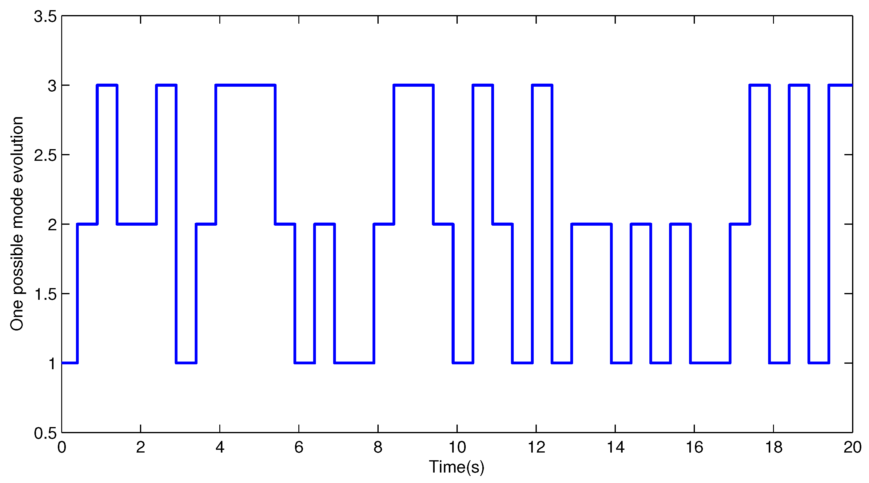
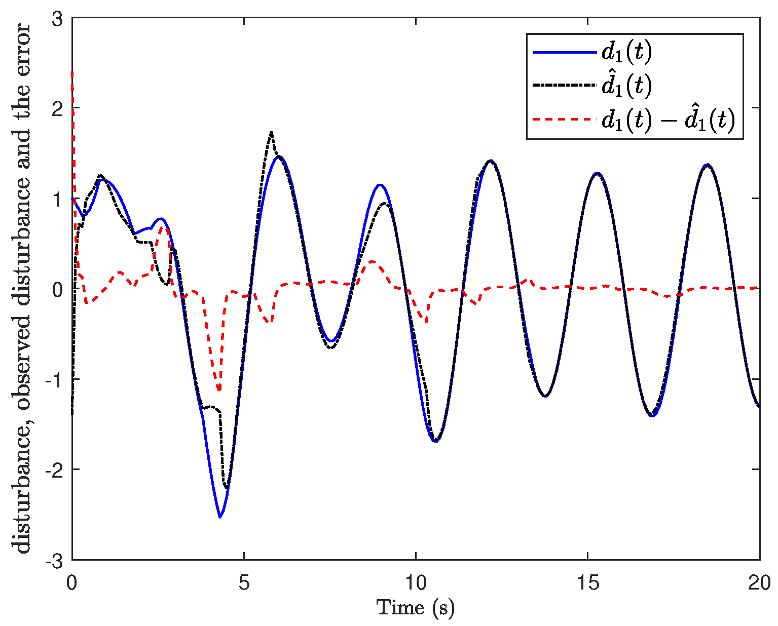
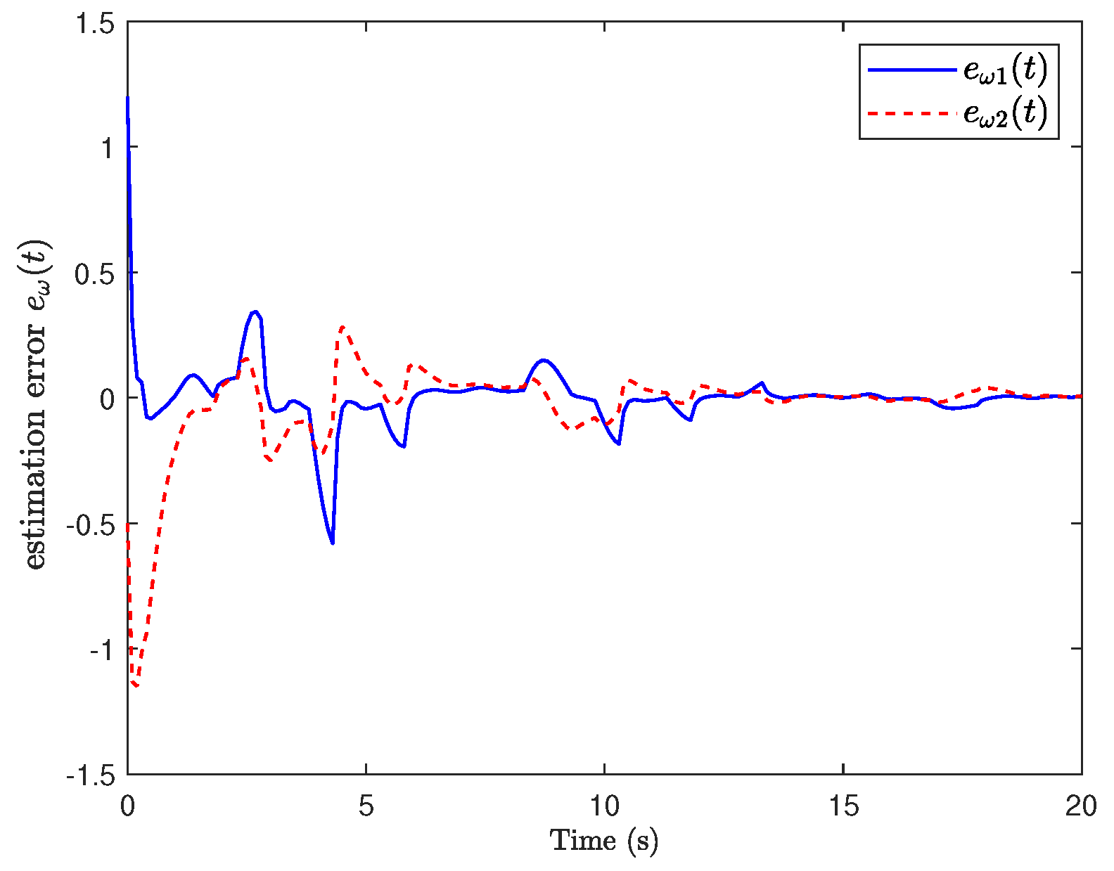
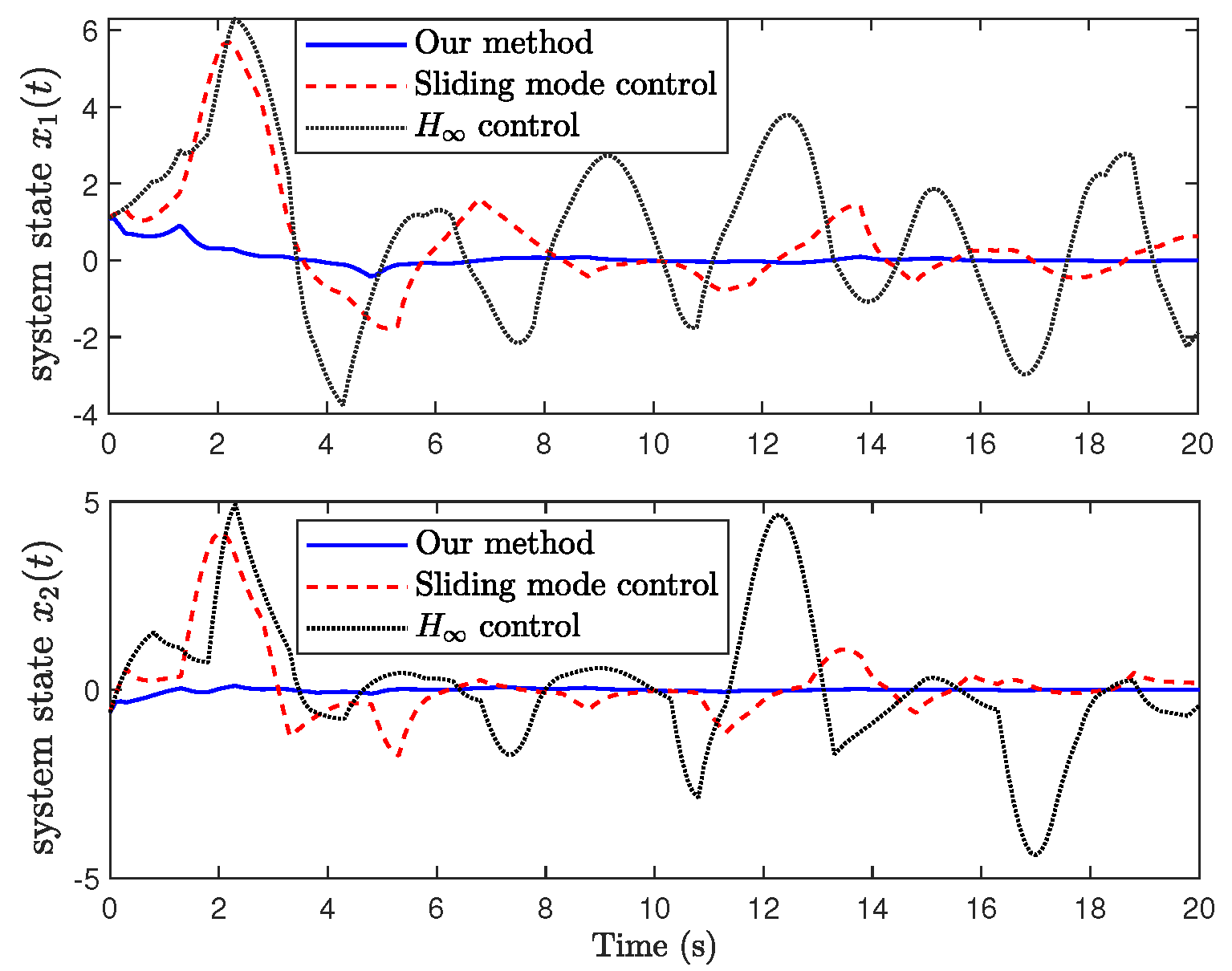
3. Simulation Results

The parameters of the system and TP matrix are given as follows:

$$\begin{array}{cc}\hfill & A_1=\left[\begin{array}{cc}-1.2& 1.5\\ 0& 0.2\end{array}\right],F_1=\left[\begin{array}{c}1.1\\ 0.1\end{array}\right],G_1=\left[\begin{array}{c}3\\ 5\end{array}\right],H_1=\left[\begin{array}{c}1.2\\ 1\end{array}\right],M_1=\left[\begin{array}{c}0.1\\ 0.1\end{array}\right],\hfill \\ \hfill & C_1=\left[\begin{array}{cc}1& 1\end{array}\right],C_{11}=\left[\begin{array}{cc}0.5& 1\end{array}\right],C_{21}=\left[\begin{array}{cc}0.2& 0\end{array}\right],V_1=\left[\begin{array}{cc}2& 0\end{array}\right],\hfill \\ \hfill & A_2=\left[\begin{array}{cc}0.6& 0.1\\ 0.5& -2.2\end{array}\right],F_2=\left[\begin{array}{c}0.2\\ 0.1\end{array}\right],G_2=\left[\begin{array}{c}8\\ 3\end{array}\right],H_2=\left[\begin{array}{c}0.6\\ 0.4\end{array}\right],M_2=\left[\begin{array}{c}0.2\\ 0.2\end{array}\right],\hfill \\ \hfill & C_2=\left[\begin{array}{cc}1& 0.5\end{array}\right],C_{12}=\left[\begin{array}{cc}1.2& 0.1\end{array}\right],C_{22}=\left[\begin{array}{cc}0.5& 0\end{array}\right],V_2=\left[\begin{array}{cc}1& 0\end{array}\right],\hfill \\ \hfill & A_3=\left[\begin{array}{cc}0.4& 0.1\\ 0.3& -1.4\end{array}\right],F_3=\left[\begin{array}{c}0.5\\ 0.2\end{array}\right],G_3=\left[\begin{array}{c}4\\ 1\end{array}\right],H_3=\left[\begin{array}{c}0.3\\ 0.4\end{array}\right],M_3=\left[\begin{array}{c}0.3\\ 0.3\end{array}\right],\hfill \\ \hfill & C_3=\left[\begin{array}{cc}0.5& 1\end{array}\right],C_{13}=\left[\begin{array}{cc}0.2& 0.5\end{array}\right],C_{23}=\left[\begin{array}{cc}0.2& 0.2\end{array}\right],V_3=\left[\begin{array}{cc}0.5& 0\end{array}\right],\hfill \\ \hfill & W_1=W_2=W_3=\left[\begin{array}{cc}0& 2\\ -2& 0\end{array}\right],U=\left[\begin{array}{cc}0& 0\\ 0& 1\end{array}\right],\prod =\left[\begin{array}{ccc}-1& 0.4& 0.6\\ ?& ?& 0.3+{\Delta }_{23}\\ 0.5& 0.4& -0.9\end{array}\right].\hfill \end{array}$$

The deception attack is considered as $\theta \left(t\right)=2tanh\left(x_1\left(t\right)\right)$, with $\mathsf{\Theta }=\left[\begin{array}{cc}2& 0\\ 0& 0\end{array}\right]$ and ${\beta }_1=0.8$. For given $\tau =10$, $b_1=b_2=b_3=b_4=1$, ${\lambda }_1={\lambda }_2=1$, ${\Delta }_{23}\in [-0.1,0.1]$, the corresponding $H_{\infty }$ performance indices obtained by different deception attack rates ${\beta }_1$ are shown in

Table 1. $H_{\infty }$ index $\gamma$ obtained by different deception attack rates ${\beta }_1$.

${\mathit{\beta }}_1$	0.3	0.5	0.8
$\gamma$	0.6134	0.7852	0.9725

. From this table, one observes that the larger the deception attack rate that is selected, the larger the $H_{\infty }$ index $\gamma$ that is obtained, which implies that more attacks are launched by adversaries and the control performance will be degraded.

Next, for simulation, the $H_{\infty }$ performance $\gamma$ and the controller and observer gains solved by Theorem 2 under ${\beta }_1=0.8$ are given as

$$\begin{array}{cc}\hfill & \gamma =0.9725,K_1=-0.1167,K_2=-0.4617,K_3=-0.2424,\hfill \\ \hfill & L_1=\left[\begin{array}{c}-0.8509\\ -0.5983\end{array}\right],L_2=\left[\begin{array}{c}-1.4175\\ -0.9852\end{array}\right],L_3=\left[\begin{array}{c}-1.1077\\ -1.0013\end{array}\right].\hfill \end{array}$$

Suppose that $f(x\left(t\right),t)=x_2\left(t\right)sin\left(t\right)$, which ensures that $\parallel f\left(x\right(t),t)\parallel \le \parallel Ux\left(t\right)\parallel$. The multiple disturbances are considered as $d_2\left(t\right)={\displaystyle \frac{6cos\left(2\pi t\right)}{5+10t}}$ and $d_3\left(t\right)=10sin\left(t\right)e^{-0.2t}$, and one possible Markov mode is drawn in Figure 1. The curves of $d_1\left(t\right)$, ${\widehat{d}}_1\left(t\right)$, and $d_1\left(t\right)-{\widehat{d}}_1\left(t\right)$ are drawn in Figure 2. Figure 3 shows the estimation error $e_{\omega }\left(t\right)$. Then, Figure 4 depicts the system state responses.

From Figure 2 and Figure 3, one can see that the disturbance observer is able to estimate the disturbance $d_1\left(t\right)$ effectively. According to Figure 4, it is observed that the matched disturbance can be observed well with the designed DOB. Then, with the utilization of estimated disturbance, the proposed composite anti-disturbance controller can stabilize the system state effectively for networked nonlinear MJSs with multiple disturbances and deception attacks.

To show the advantages of the proposed method and some existing methods, the comparison results are depicted in the following figures.

Specifically, the comparison results with the traditional $H_{\infty }$ control and sliding mode control are depicted in Figure 5. From this figure, it is seen that our proposed composite anti-disturbance control method is able to achieve better control performance than the traditional $H_{\infty }$ control and sliding mode control. To be specific, the convergence time of the state responses under our method is about 6 s, while the system responses do not converge to steady state under $H_{\infty }$ control and sliding mode control. Meanwhile, the maximum overshoots for the first state $x_1\left(t\right)$ and the second state $x_1\left(t\right)$ obtained by our method are 1.2 and 0.5, respectively, which are much less than the corresponding values obtained by $H_{\infty }$ control, with 6.2 and 4.9, and sliding mode control, with 5.7 and 4.1. In addition, it is fair to say that the computational complexity of our composite anti-disturbance control approach is higher than the other two methods due to the extra design of the disturbance observer and the estimated disturbance added in the controller.

Then, the actual values of the $H_{\infty }$ index obtained by our composite anti-disturbance static output control method and traditional $H_{\infty }$ control method are compared in Figure 6. From this figure, it is seen that the index $\gamma$ converges to 0.5682 under our method, which is less than the theoretical value $\gamma =0.9725$. However, under the traditional $H_{\infty }$ control method, the system state can not be stabilized as the existence of matched disturbance $d_1\left(t\right)$ and the index $\gamma$ diverges. This further confirms the advantage of our proposed control method.

Next, the number of design variables in the control strategy and number of stability conditions under our static output control method and existing dynamic output control method [26] are compared in

Table 2. The comparisons between our method and the existing method [26].

Methods	Our Method	Existing Method [26]
Number of design variables in control strategy	3	27
Number of stability analysis conditions	3	3

. In terms of this table, it is seen that fewer design variables are required in our method than the existing method [26], and the same stability analysis conditions are obtained, which indicates that the computational complexity of our method is much lower than [26]. The reason is that the dynamic output control requires more controller gains and Lyapunov variables than the static output control.

Finally, Figure 7 shows the compared state responses of the closed-loop system with the designed composite anti-disturbance controller and the standard static output controller (8). It is observed that the system state responses can be controlled well by our designed controller while they are unstable under the standard static output controller without considering disturbance compensation and deception attacks. This further confirms the effectiveness of the proposed control method for stabilizing the system under multiple disturbances and deception attacks.

In this simulation, the practical problems like multiple disturbances and deception attacks of networked nonlinear MJSs were considered. However, some other common issues, such as communication delays and packet dropouts in network channels, were not taken into account. Furthermore, the limited bandwidth of real-world communication networks is ignored, which could lead to network congestion when large numbers of signals are transmitted in short times. In order to obtain more practical and accurate results, the above issues can be considered in the simulation setup in our following research.

4. Conclusions

In this article, the composite anti-disturbance static output control issue was addressed for nonlinear MJSs with general TPs against multiple disturbances and deception attacks. Based on the constructed composite anti-disturbance static output controller, the matched and mismatched disturbances can be compensated and attenuated, respectively. In terms of the Finsler lemma, sufficient LMIs conditions were established to ensure the system stability and the required performance. The validity of the developed approach was testified via several numerical simulations. The fact that the controller gains may be sensitive to implementation error or disturbances in practical environments could lead to some uncertainties in accurate controller values and degradation of the control performance. Therefore, in our future work, the nonfragile controller design problem will be investigated to reduce the sensitivity of the controller uncertainties on control performance, and to increase the controller robustness. Furthermore, as the effectiveness of the proposed control method is verified via a numerical simulation system, its application to some practical systems like power systems [29], robotic systems [30], and unmanned surface vehicles [31] will be investigated in the future to increase its feasibility to real-world scenarios.

References

1. Shi, P.; Liu, M.; Zhang, L. Fault-tolerant sliding-mode-observer synthesis of Markovian jump systems using quantized measurements. IEEE Trans. Ind. Electron. 2015, 62, 5910–5918. [Google Scholar] [CrossRef]
2. Wang, B.; Zhu, Q. The stabilization problem for a class of discrete-time semi-Markov jump singular systems. Automatica 2025, 171, 111960. [Google Scholar] [CrossRef]
3. Tartaglione, G.; Ariola, M.; Amato, F. An observer-based output feedback controller for the finite-time stabilization of Markov jump linear systems. IEEE Control Syst. Lett. 2019, 3, 763–768. [Google Scholar] [CrossRef]
4. Tan, Y.; Liu, J.; Xie, X.; Tian, E.; Liu, J. Dynamic-memory event-triggered sliding-mode secure control for nonlinear semi-Markov jump systems with stochastic cyber attacks. IEEE Trans. Autom. Sci. Eng. 2024, 21, 202–214. [Google Scholar] [CrossRef]
5. Cao, Z.; Niu, Y.; Zou, Y. Adaptive neural sliding mode control for singular semi-Markovian jump systems against actuator attacks. IEEE Trans. Syst. Man Cybern. Syst. 2019, 51, 1523–1533. [Google Scholar] [CrossRef]
6. Zong, G.; Ren, H. Guaranteed cost finite-time control for semi-Markov jump systems with event-triggered scheme and quantization input. Int. J. Robust Nonlinear Control 2019, 29, 5251–5273. [Google Scholar] [CrossRef]
7. Shen, M.; Gu, Y.; Zhu, S.; Zong, G.; Zhao, X. Mismatched quantized H output-feedback control of fuzzy Markov jump systems with a dynamic guaranteed cost triggering scheme. IEEE Trans. Fuzzy Syst. 2023, 32, 1681–1692. [Google Scholar] [CrossRef]
8. Li, X.; Zhang, W.; Lu, D. Stability and stabilization analysis of Markovian jump systems with generally bounded transition probabilities. J. Frankl. Inst. 2020, 357, 8416–8434. [Google Scholar] [CrossRef]
9. Zhang, L.; Boukas, E.K. Stability and stabilization of Markovian jump linear systems with partly unknown transition probabilities. Automatica 2009, 45, 463–468. [Google Scholar] [CrossRef]
10. Shen, M.; Ye, D.; Wang, Q.G. Event-triggered H filtering of Markov jump systems with general transition probabilities. Inf. Sci. 2017, 418, 635–651. [Google Scholar] [CrossRef]
11. Liu, X.; Ma, G.; Pagilla, P.R.; Ge, S.S. Dynamic output feedback asynchronous control of networked Markovian jump systems. IEEE Trans. Syst. Man Cybern. Syst. 2018, 50, 2705–2715. [Google Scholar] [CrossRef]
12. Antunes, D.J.; Qu, H. Frequency-domain analysis of networked control systems modeled by Markov jump linear systems. IEEE Trans. Control Netw. Syst. 2021, 8, 906–916. [Google Scholar] [CrossRef]
13. Yan, S.; Gu, Z.; Park, J.H.; Shen, M. Fusion-based event-triggered H state estimation of networked autonomous surface vehicles with measurement outliers and cyber-attacks. IEEE Trans. Intell. Transp. Syst. 2024, 25, 7541–7551. [Google Scholar] [CrossRef]
14. Yan, S.; Gu, Z.; Park, J.H.; Xie, X.; Dou, C. Probability-density-dependent load frequency control of power systems with random delays and cyber-attacks via circuital implementation. IEEE Trans. Smart Grid 2022, 13, 4837–4847. [Google Scholar] [CrossRef]
15. Guo, L.; Chen, W. Disturbance attenuation and rejection for systems with nonlinearity via DOBC approach. Int. J. Robust Nonlinear Control 2005, 15, 109–125. [Google Scholar] [CrossRef]
16. Wang, B.; Zhu, Q.; Li, S. Stabilization of discrete-time hidden semi-Markov jump linear systems with partly unknown emission probability matrix. IEEE Trans. Autom. Control 2024, 69, 1952–1959. [Google Scholar] [CrossRef]
17. Chen, M.; Shi, P.; Lim, C.C. Robust constrained control for MIMO nonlinear systems based on disturbance observer. IEEE Trans. Autom. Control 2015, 60, 3281–3286. [Google Scholar] [CrossRef]
18. Ding, K.; Zhu, Q. Extended dissipative anti-disturbance control for delayed switched singular semi-Markovian jump systems with multi-disturbance via disturbance observer. Automatica 2021, 128, 109556. [Google Scholar] [CrossRef]
19. Wang, F.; Gao, H.; Wang, K.; Zhou, C.; Zong, Q.; Hua, C. Disturbance observer-based finite-time control design for a quadrotor UAV with external disturbance. IEEE Trans. Aerosp. Electron. Syst. 2020, 57, 834–847. [Google Scholar] [CrossRef]
20. Alhelou, H.H.; Parthasarathy, H.; Nagpal, N.; Agarwal, V.; Nagpal, H.; Siano, P. Decentralized stochastic disturbance observer-based optimal frequency control method for interconnected power systems with high renewable shares. IEEE Trans. Ind. Inform. 2021, 18, 3180–3192. [Google Scholar]
21. Ding, S.; Hou, Q.; Wang, H. Disturbance-observer-based second-order sliding mode controller for speed control of PMSM drives. IEEE Trans. Energy Convers. 2022, 38, 100–110. [Google Scholar] [CrossRef]
22. Liu, Y.; Wang, H.; Guo, L. Composite robust H control for uncertain stochastic nonlinear systems with state delay via a disturbance observer. IEEE Trans. Autom. Control 2018, 63, 4345–4352. [Google Scholar] [CrossRef]
23. Yao, X.; Guo, L. Composite anti-disturbance control for Markovian jump nonlinear systems via disturbance observer. Automatica 2013, 49, 2538–2545. [Google Scholar] [CrossRef]
24. Zhao, Y.; Li, X.; Song, S. Observer-based sliding mode control for stabilization of mismatched disturbance systems with or without time delays. IEEE Trans. Syst. Man Cybern. Syst. 2021, 51, 7337–7345. [Google Scholar] [CrossRef]
25. Hwang, S.; Kim, H.S. Extended disturbance observer-based integral sliding mode control for nonlinear system via T–S fuzzy model. IEEE Access 2020, 8, 116090–116105. [Google Scholar] [CrossRef]
26. Yao, X.; Guo, L. Composite disturbance-observer-based output feedback control and passive control for Markovian jump systems with multiple disturbances. IET Control Theory Appl. 2014, 8, 873–881. [Google Scholar] [CrossRef]
27. Boyd, S.P.; Ghaoui, L.E.; Feron, E.; Balakrishnan, V. Linear Matrix Inequalities in Systems and Control Theory; SIAM: Philadelphia, PA, USA, 1994. [Google Scholar]
28. Wang, Y.; Xie, L.; de Souza, C.E. Robust control of a class of uncertain nonlinear systems. Syst. Control Lett. 1992, 19, 139–149. [Google Scholar] [CrossRef]
29. Yan, S.; Gu, Z.; Park, J.H.; Xie, X. Sampled memory-event-triggered fuzzy load frequency control for wind power systems subject to outliers and transmission delays. IEEE Trans. Cybern. 2023, 53, 4043–4053. [Google Scholar] [CrossRef]
30. Yao, X.; Zhang, L.; Zheng, W.X. Uncertain disturbance rejection and attenuation for semi-Markov jump systems with application to 2-degree-freedom robot arm. IEEE Trans. Circuits Syst. Regul. Pap. 2021, 68, 3836–3845. [Google Scholar] [CrossRef]
31. Yan, S.; Gu, Z.; Ahn, C.K. Memory-event-triggered H filtering of unmanned surface vehicles with communication delays. IEEE Trans. Circuits Syst. II Express Briefs 2021, 68, 2463–2467. [Google Scholar] [CrossRef]
Figure 1. One possible Markov mode.
Symmetry 17 00658 g001
Figure 2. The disturbance. d 1 ( t ) , estimation d ^ 1 ( t ) , and d 1 ( t ) d ^ ( t ) .
Symmetry 17 00658 g002
Figure 3. The estimation error e ω ( t ) .
Symmetry 17 00658 g003
Figure 4. The system state responses under our composite anti-disturbance static output controller (6).
Symmetry 17 00658 g004
Figure 5. The system state responses under our method, traditional H control, and sliding mode control.
Symmetry 17 00658 g005
Figure 6. The actual values of H index γ under different methods.
Symmetry 17 00658 g006
Figure 7. The system state responses under our method and the standard static output controller (8).
Symmetry 17 00658 g007