On Design of IIR Cascaded-Resonator-Based Complex Filter Banks

Abstract

This paper extends the research on cascaded-resonator (CR)-based filter banks introduced in previous studies. These IIR filter banks are online adaptive, making them highly suitable for spectral decomposition and signal analysis. The multiple-resonator-based structure offers an efficient design with low side lobes and high stopband attenuation. While earlier works focused on the fundamental structure and principles of these filter banks, the efficiency of their design was not thoroughly explored. In this study, thanks to the full periodicity of the frequency response, significant improvements in the modeling of the characteristic polynomial (the denominator of the transfer function) and preprocessing filters are introduced, resulting in an enhanced sparsity and a computational efficiency. Additionally, the previously employed linear programming algorithm for solving semi-infinite problems including a large number of linear constraints is replaced by more advanced quadratic programming (QP) or linear least-squares (LLS) optimization methods. These changes lead to a much faster and more powerful design process, even for filter banks with a larger number of resonator cascades and/or resonators per cascade. Furthermore, additional enhancements to the design methodology are proposed, further improving the robustness and applicability of the filters. These advancements enable the creation of highly efficient filter banks capable of handling complex and dynamic spectral analysis tasks in real time.

1. Introduction

Filter banks are essential components in a wide range of engineering applications, such as speech analysis, bandwidth reduction, radar and sonar signal processing, spectral parameterization, adaptive noise suppression, and sub-band coding. Functioning as arrays of digital bandpass filters that share either a common input or output, filter banks are fundamental to both the analysis and synthesis stages of signal processing systems. Complex filter banks, which leverage complex-valued transfer functions and coefficients, have demonstrated superior performance in tasks where the separation of amplitude and phase information is critical. These applications extend to telecommunications, adaptive filtering, and speech processing, enabling efficient representation and interpretation of signal dynamics.

Introducing adaptability into filter banks allows them to dynamically adjust their characteristics in real time, significantly broadening their utility. This adaptability is commonly achieved using algorithms such as least mean squares (LMS), recursive least squares (RLS), or modern machine-learning-inspired methods. These adaptive approaches, coupled with complex transfer functions, provide considerable advantages in tasks like channel equalization, interference cancellation, and beamforming [1,2]. Furthermore, advances in computational capabilities have made real-time implementation of adaptive filter banks feasible, even in resource-constrained environments. Practical implementations include their use in echo cancellation systems, speech enhancement, and dynamic spectrum management in cognitive radio systems.

Among the most promising developments in this field are resonator-based filter banks, particularly cascaded-resonator (CR)-based filters. These filters have shown exceptional potential in spectral decomposition and signal analysis due to their efficient structures and desirable frequency characteristics, including low side lobes and high stopband attenuation. Previous studies have explored their application in infinite-impulse-response (IIR) systems for adaptive spectral analysis, utilizing symmetrical pole placement to achieve uniform harmonic frequency responses [3,4]. However, while these studies laid a strong foundation, challenges in computational complexity and design efficiency remained.

This paper builds on earlier work by addressing key limitations in the design and implementation of CR-based filter banks. To overcome these challenges, we propose a series of methodological improvements that serve as the primary research objectives of this work. Specifically, by leveraging the full periodicity of the frequency responses, we enhance the modeling of the characteristic polynomial (i.e., the denominator of the transfer function) and introduce more efficient preprocessing filters, resulting in significantly sparser filter structures. These advancements reduce computational demands and improve the adaptability of the filter banks for real-time applications. Based on previous experience with linear programming (LP) methods in earlier research, the current study adopts quadratic programming (QP) and linear least-squares (LLS) approaches as more computationally efficient alternatives. These methods offer improved scalability and allow for faster optimization, especially in the design of higher-order filter banks. Additionally, the use of faster optimization algorithms—quadratic programming (QP) and linear least-squares (LLS)—in place of previously used linear programming further accelerates the design process and enables the use of higher-order resonators and additional cascades. Altogether, the proposed methodological enhancements result in more robust, efficient, and flexible filter banks capable of handling complex spectral analysis tasks in real time.

The practical applications of CR-based filter banks underscore their importance. One key application is in speech signal analysis and speaker recognition, where the ability to conduct precise, real-time analysis of speech frequencies facilitates the generation of probabilistic frequency profiles unique to individual speakers. This capability has significant implications for user authentication, security, and advanced communication systems.

Another critical domain is audiometry and hearing correction. Modern audiometric techniques demand high-resolution frequency analysis to diagnose hearing impairments and design advanced hearing aids. The proposed improvements in CR-based filter banks allow for the creation of high-resolution audiograms with up to 96 center frequencies, catering to the needs of state-of-the-art hearing aids. By dynamically adapting to auditory environments, these filter banks enhance the auditory experience of individuals with severe hearing impairments, enabling them to perform complex auditory tasks such as enjoying music.

Proposed CR-based filter banks can be adapted for real-time applications in dynamic environments like cognitive radio systems by implementing adaptive algorithms that can adjust to varying spectral conditions. Since cognitive radio systems require flexibility to dynamically access different frequency bands, the CR-based filter banks can be designed to quickly reconfigure their filter characteristics based on the environment’s spectrum. This can be achieved through real-time feedback loops and signal processing techniques, allowing the system to efficiently detect and utilize available spectrum, thus enhancing the performance of cognitive radio systems while maintaining low latency and optimal resource usage.

Beyond these applications, CR-based filter banks also have potential in underwater acoustic communication systems, where adaptability to dynamic signal characteristics is essential. Their real-time adaptability and spectral precision make them well suited to such challenging environments.

In conclusion, the advancements presented in this paper address critical limitations of earlier CR-based filter bank designs while broadening their applicability. By combining theoretical improvements with practical applications, this work enhances the computational efficiency and adaptability of these systems, reinforcing their relevance across a diverse range of engineering and biomedical fields.

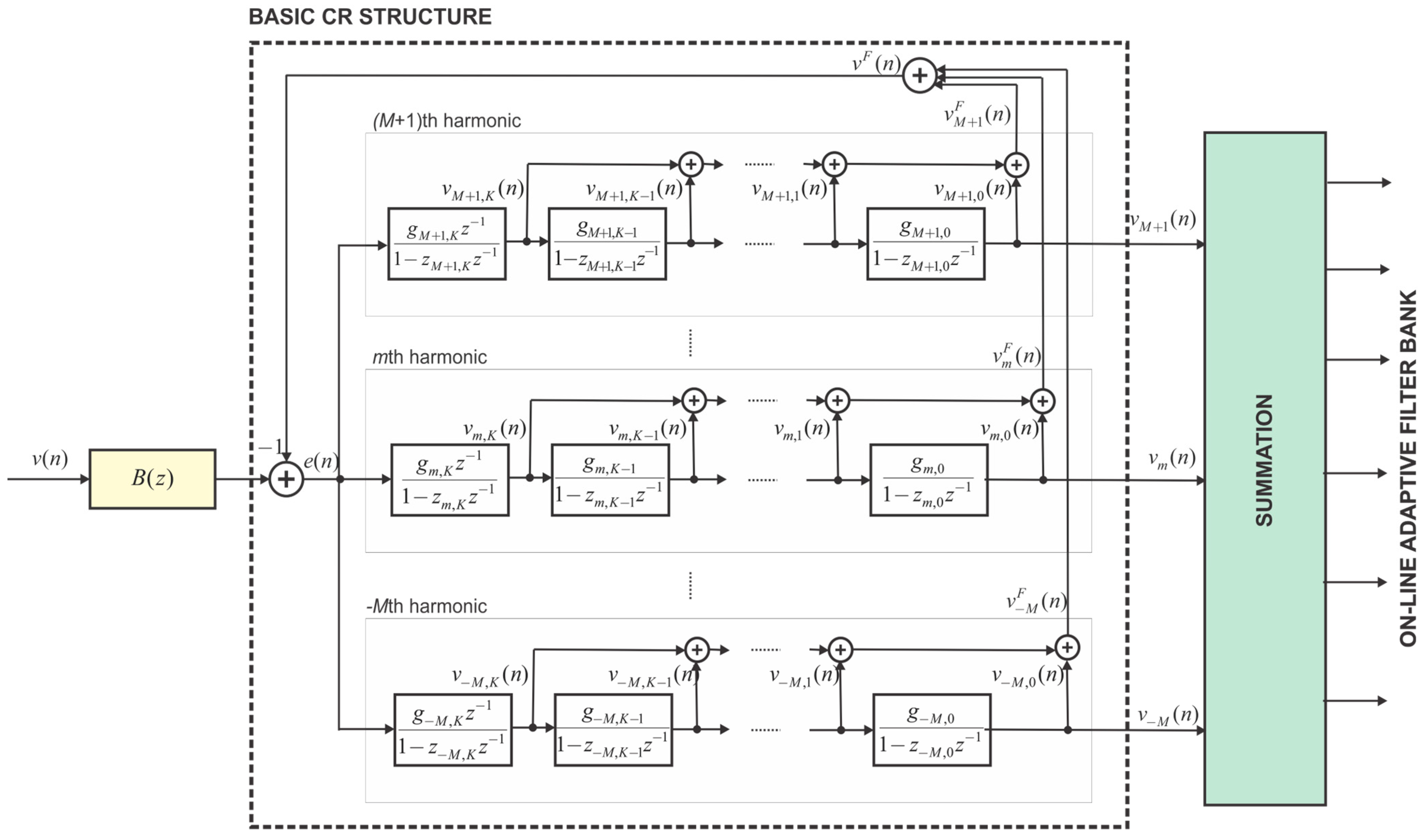
2. CR-Based Structure

The CR-based structure consists of resonator cascades connected parallel and embedded in common feedback. The block diagram of the $K$-type CR-based structure consisting of $K+1$ resonators serially connected in each of $2M+2$ cascades is shown in Figure 1. Each cascade contains $K+1$ complex poles positioned on the unit circle, centered around the corresponding harmonic frequency. Associated with each resonator are complex gains $\left\{g_{m,k},m=-M,\dots ,0,\dots ,M+1,k=0,1,\dots ,K\right\}$, corresponding to poles $\left\{z_{m,k},m=-M,\dots ,0,\dots ,M+1,k=0,1,\dots ,K\right\}$. The closed-loop transfer function for harmonic $m$ is given by the following expression [3]:

$$H_m^{AB}\left(z\right)={\displaystyle \frac{V_m\left(z\right)}{V\left(z\right)}}=g_{m,0}^{\prime }{\displaystyle \frac{{z^{-1}P}_m\left(z\right)B\left(z\right)}{A\left(z\right)}}=H_m\left(z\right){\displaystyle \frac{B\left(z\right)}{A\left(z\right)}}$$

(1)

where $z=e^{j\omega }$, $\omega =2\pi f/f_S$, $f_S$ is the sampling rate, and $f_1$ is the fundamental frequency.

$$H_m\left(z\right)=g_{m,0}^{\prime }{z^{-1}P}_m\left(z\right)$$

(2)

where

$$P_m\left(z\right)=\prod _{\begin{array}{c}n=-M\\ n\ne m\end{array}}^{M+1}\prod _{i=0}^K\left(1-z_{n,i}{z}^{-1}\right),{ g}_{m,k}^{\prime }=\prod _{i=k}^K{g}_{m,i},$$

(3)

It is very important to note that both polynomials $B\left(z\right)$ and $A\left(z\right)$ have periodical frequency responses with a period equal to the sampling frequency divided by the number of harmonic cascades, $2M+2,$ because they are present in the frequency responses of all harmonics (channels), which have to have the same shapes. This periodicity results in a very small number of filter nonzero-coefficients. Only the $\left(2M+2\right)$-th coefficient is different from zero. This important feature can be used for reduction in length of vector of unknown variables during design procedure. In addition, an implementation of the preprocessing filter $B\left(z\right)$ is much ($2M+2$ times) faster. Bearing this in mind, we can assume the following form of $B\left(z\right)$ and $A\left(z\right)$:

$$\begin{gathered} B\left(z\right)=b_0^R+b_1^R{z}^{-(2\mathrm{M}+2)}+\cdots +b_{N_B^R-1}^R{z}^{-\left(N_B^R-1\right)(2\mathrm{M}+2)}+b_{N_B^R}{z}^{-N_B^R(2\mathrm{M}+2)} \\ A\left(z\right)=1+a_1^R{z}^{-(2\mathrm{M}+2)}+\cdots +a_{N_a^R-1}^R{z}^{-\left(N_A^R-1\right)\left(2\mathrm{M}+2\right)}+a_{N_A^R}{z}^{-N_A^R(2\mathrm{M}+2)} \end{gathered}$$

(4)

It is notable that $N_B=N_B^R(2M+2)$ and $N_A=N_A^R(2M+2)$ where $N_B$ and $N_A$ are orders of $B\left(z\right)$ and $A\left(z\right)$, respectively. It means that $2M+2$ times fewer coefficients have to be calculated than in the case when all filter coefficients are supposed unknown and have to be found. The polynomial $A\left(z\right)$ is of the order $N_A=\left(K+1\right)\left(2M+2\right)$, which implies a reduced order, i.e., $N_A^R=K+1.$ It is important to note that, due to symmetry, the order $N_B$ of the polynomial $B\left(z\right)$ must be a multiple of the number of harmonic cascades, i.e., $2M+2$. In addition to that, an implementation of the FIR filter $B\left(z\right)$ is extremely easier due to its sparsity. The sparsity of characteristic polynomial $A\left(z\right)$ does not influence on the implementation but on the values of the gains $g_{m,k}$ only.

It should be noted that the common feedback loop transforms all resonator poles into zeros in the transfer functions $H_m\left(z\right)$, except for those originating from channel $m$, which are inherently canceled by their corresponding pole-generating mechanisms.

An important observation is that increasing the number of resonators in the cascade enhances stopband attenuation and reduces side lobes [3]. However, a higher $K$ value also results in a higher filter order, longer response time, and increased computational complexity.

3. Design Method

3.1. Problem Statement

A key characteristic of the mother filter bank $\left\{H_m\left(z\right),m=-M,\dots ,0,\dots ,M+1\right\}$ is that the phase difference between adjacent filters is $\left(K+1\right)\pi$ within the frequency band between their center frequencies—specifically, zero for odd $K$, and $\pi$ for even $K$—and zero elsewhere. The main concept involves superimposing the frequency responses of a group of adjacent harmonics: using a “+” sign for odd $K$, and alternating “–” and “+” signs for even $K$.

A virtual, composite transfer function $H\left(z\right)$ is constructed by combining segments of the individual transfer functions, corresponding to the frequency bands between two adjacent harmonic frequencies. For each pair of neighboring harmonics, $m$ and $m+1$, their combined response over the band $\left(m{f}_1,\left(m+1\right)f_1\right)$ is defined as

$$H\left(z\right)=H_m\left(z\right)\mp H_{m+1}\left(z\right)=z^{-1}\left[g_{m,0}^0{P}_m\left(z\right)\mp {g_{m+\mathrm{1,0}}^{0}P}_{m+1}\left(z\right)\right],$$

(5)

for $f\in \left(m{f}_1,\left(m+1\right)f_1\right)$, where $m=-M,\dots ,0,\dots ,M+1$, and the gain coefficients $g_{m,0}^0=z_m/P_m\left(z_m\right)$, for $m=-M,\dots ,0,\dots ,M+1$, ensure unity gains in the frequencies $m{f}_1$ and $\left(m+1\right)f_1$. The minus sign ($-$) is applied for even $K$ (i.e., $K=0,2,4,\dots$ ), and the plus sign ($+$) is used for an odd $K$ (i.e., $K=1,3,5,\dots$).

It is also important to mention that for $m=M+1$, the corresponding frequency band becomes $f\in \left(-\left(M+1\right)f_1,-M{f}_1\right)$ and the function simplifies to $H\left(z\right)=H_{M+1}\left(z\right)\mp H_{-M}\left(z\right)$.

In cases where the output filter bandwidth spans more than two harmonic bands, there may be interference from harmonics of order less than $m$ or greater than $m+1$ within the band $\left(m{f}_1,\left(m+1\right)f_1\right)$. This influence, however, is generally negligible, particularly for larger values of $K$.

$$\begin{array}{c}{H}^{\prime }\left(z\right)=H_m\left(z\right)\mp H_{m+1}\left(z\right)+H_{m+2}\left(z\right)\\ =z^{-1}\left[g_{m,0}^0{P}_m\left(z\right)\mp {g_{m+\mathrm{1,0}}^{0}P}_{m+1}\left(z\right)+{g_{m+\mathrm{2,0}}^{0}P}_{m+2}\left(z\right)\right],\end{array}$$

(6)

Again, as in (5), the “$-$” is used for an even $K$ ($K=0,2,4,\dots$), and “$+$” is used for an odd $K$ ($K=1,3,5,\dots$). Note that for $m=M+1$, $f\in \left(-\left(M+1\right)f_1,-M{f}_1\right)$ and $H^{\prime }\left(z\right)=H_{M+1}\left(z\right)\mp H_{-M}\left(z\right)+H_{-M+1}\left(z\right)$.

The group delay (in samples) and phase response of $H\left(z\right)$ are ${\tau }_H=\left(K+1\right)\left(2M+2\right)/2$ and $\mathrm{a}\mathrm{r}\mathrm{g}\left(H\left(z\right)\right)={\tau }_H\left(\omega -m{\omega }_1\right)$, respectively.

The corresponding desired linear phase transfer function is defined as follows

$$H^d\left(z\right)=e^{-j\left[{\tau }_H\left(\omega -m{\omega }_1\right)+{\tau }_B\omega \right]},$$

(7)

$$\mathrm{for} f\in \left(m{f}_1,\left(m+1\right)f_1\right),m=-M, \dots ,0, \dots ,M+1,$$

The desired group delay is increased by a fixed amount ${\tau }_B$, which arises due to the presence of $B\left(z\right)/A\left(z\right)$, where the delay is a multiple of $N_B$.

Our goal is to find causal stable rational functions $H^{AB}\left(z\right)=H\left(z\right)B\left(z\right)/A\left(z\right)$ and $H^{AB\prime }\left(z\right)=H^{\prime }\left(z\right)B\left(z\right)/A\left(z\right)$ that best approximate $H^d\left(z\right)$ in the defined least-squares sense.

The basic weighted least-squares formulation for stable IIR filters is given by

$$J_2\left(\mathit{x}\right)=\sum _{i=0}^{N_F-1}W\left(z_i\right)\left\{{\left|{\displaystyle \frac{H\left(z_i\right)B\left(z_i\right)}{A\left(z_i\right)}}-H^d\left(z_i\right)\right|}^2+{\left|{\displaystyle \frac{H\prime \left(z_i\right)B\left(z_i\right)}{A\left(z_i\right)}}-H^d\left(z_i\right)\right|}^2\right\}$$

(8)

Since $H\left(z\right)$ and $H^{\prime }\left(z\right)$ are defined in terms of poles $\left\{z_{m,k}\right\}$, with $m=-M,\dots ,0,\dots ,M+1$ and $k=0,1,\dots ,K$, it is necessary to determine the coefficients of the filter $B\left(z\right)/A\left(z\right)$. Once $A\left(z\right)$ is established, the corresponding gains $g_{m,k}^{\prime }$, and $g_{m,k}$ can be computed accordingly.

3.2. Linearization

The optimization problem in (8) poses two notable technical challenges. First, the presence of the denominator polynomial $A\left(z\right)$ transforms (8) into a constrained rational approximation problem, introducing a significant degree of nonlinearity. Second, the stability constraint imposes a requirement that the zeros of $A\left(z\right)$ remain strictly within the unit circle. This constraint is particularly challenging to handle, as the relationship between the zeros of a high-order polynomial and its coefficients is both implicit and highly nonlinear [5].

One convenient property of the characteristic polynomial $A\left(z\right)$, as defined in Equation (4), is that it inherently exhibits a periodic frequency response with a period equal to the sampling frequency divided by the number of harmonic cascades, $2M+2$. In most optimization scenarios, this periodicity helps ensure that the poles remain inside the unit circle, thereby resulting in stable transfer functions. Consequently, stability is considered a given, and constraints related to ensuring stability will not be explicitly addressed in the subsequent discussion. This assumption greatly simplifies the optimization process by eliminating the need to account for potential stability violations. It also avoids common pitfalls such as becoming trapped in local minima or encountering convergence issues. Moreover, this approach significantly reduces the computational complexity and time required for optimization, making the process more efficient and streamlined while maintaining reliable results.

The linearized iterative approximation model can be constructed by using $A^{\left(k-1\right)}\left(z\right)$, obtained from the previous optimization iteration $k-1$, as a part of the weighting function [6,7,8].

$$J_2\left(\mathit{x}\right)=\sum _{i=0}^{N_F-1}W\left(z_i\right)\left\{{{\displaystyle \frac{\left|H\left(z_i\right)B\left(z_i\right)-A^{\left(k\right)}\left(z_i\right)H^d\left(z_i\right)\right|}{{\left|A^{\left(k-1\right)}\left(z_i\right)\right|}^2}}}^2+{{\displaystyle \frac{\left|H\prime \left(z_i\right)B\left(z_i\right)-A^{\left(k\right)}\left(z_i\right)H^d\left(z_i\right)\right|}{{\left|A^{\left(k-1\right)}\left(z_i\right)\right|}^2}}}^2\right\}$$

(9)

where $A^{\left(k\right)}\left(z\right)$ and $A^{\left(k-1\right)}\left(z\right)$ represent the characteristic polynomial $A\left(z\right)$ at iterations $k$ and $k-1$, respectively, and $W\left(z\right)$ denotes the selected weighing function. It is important to note that $J_2\left(\mathit{x}\right)$ in (9) is a quadratic function of the filter coefficients. Consequently, least-squares designs of IIR filters can be efficiently achieved using iterative quadratic programming (QP) or linear least-squares (LLS) techniques.

The above equality can be expressed as

$$\begin{array}{cc}{J}_2\left(\mathit{x}\right)={\displaystyle \sum _{i=0}^{N_F-1}}& W\left(z_i\right)\{{\displaystyle \frac{{\left|\left[{\left.{H\left(z_i\right)\mathit{q}}_{\mathit{B}}\right|}_{z=z_i},{\left.-H^d\left(z_i\right){\mathit{q}}_{\mathit{A}}\right|}_{z=z_i}\right]\mathit{x}-H^d\left(z_i\right)\right|}^2}{{\left|A^{\left(k-1\right)}\left(z_i\right)\right|}^2}}\\ & +{\displaystyle \frac{{\left|\left[{\left.{H^{\prime }\left(z_i\right)\mathit{q}}_{\mathit{B}}\right|}_{z=z_i},{\left.-H^d\left(z_i\right){\mathit{q}}_{\mathit{A}}\right|}_{z=z_i}\right]\mathit{x}-H^d\left(z_i\right)\right|}^2}{{\left|A^{\left(k-1\right)}\left(z_i\right)\right|}^2}}\}\hfill \\ & ={\displaystyle \sum _{i=0}^{N_F-1}}\left\{{\left|{\mathit{h}}_{\mathit{i}}\mathit{x}-g_{\mathit{i}}\right|}^2+{\left|{\mathit{h}}_{\mathit{i}}^{\prime }\mathit{x}-g_{\mathit{i}}\right|}^2\right\}\hfill \end{array}$$

(10)

where

$\mathit{x}={\left[\begin{array}{cc}{{\mathit{x}}_{\mathit{B}}}^T& {{\mathit{x}}_{\mathit{A}}}^T\end{array}\right]}^T$,

${\mathit{x}}_{\mathit{B}}={\left[\begin{array}{cccc}{b}_0^R& b_1^R& b_2^R& \cdots \end{array}\begin{array}{ccc} & b_{N_B^R-1}^R& b_{N_B^R}^R\end{array}\right]}^T$,

${\mathit{x}}_{\mathit{A}}={\left[\begin{array}{cc}{a}_1^R& a_2^R\end{array} \cdots \begin{array}{cc}{a}_{N_A^R-1}^R& a_{N_A^R}^R\end{array}\right]}^T$,

${\mathit{q}}_{\mathit{B}}=\left[\begin{array}{ccc}1& z^{-\left(2M+2\right)}& z^{-2\left(2M+2\right)}\end{array} \begin{array}{ccc}\cdots & z^{-\left(N_B^R-1\right)\left(2M+2\right)}& z^{-N_B^R\left(2M+2\right)}\end{array}\right]$,

${\mathit{q}}_{\mathit{A}}=\left[\begin{array}{cc}{z}^{-\left(2M+2\right)}& z^{-2\left(2M+2\right)}\end{array} \begin{array}{ccc}\cdots & z^{-\left(N_A^R-1\right)\left(2M+2\right)}& z^{-N_A^R\left(2M+2\right)}\end{array}\right]$,

$$\begin{array}{cc}{\mathit{h}}_i={\displaystyle \frac{\sqrt{W\left(z_i\right)}\left[{\left.{H\left(z_i\right)\mathit{q}}_{\mathit{B}}\right|}_{z=z_i},{\left.-H^d\left(z_i\right){\mathit{q}}_{\mathit{A}}\right|}_{z=z_i}\right]}{\left|A^{\left(k-1\right)}\left(z_i\right)\right|}}& g_i={\displaystyle \frac{\sqrt{W\left(z_i\right)}{H}^d\left(z_i\right)}{\left|A^{\left(k-1\right)}\left(z_i\right)\right|}}\\ {\mathit{h}}_{\mathit{i}}^{\prime }={\displaystyle \frac{\sqrt{W\left(z_i\right)}\left[{\left.{H^{\prime }\left(z_i\right)\mathit{q}}_{\mathit{B}}\right|}_{z=z_i},{\left.-H^d\left(z_i\right){\mathit{q}}_{\mathit{A}}\right|}_{z=z_i}\right]}{\left|A^{\left(k-1\right)}\left(z_i\right)\right|}}& \end{array}$$

Further, $J_2\left(\mathit{x}\right)$ in (10) can be expressed as

$$J_2\left(\mathit{x}\right)={\displaystyle \frac{1}{2}}{\mathit{x}}^T\mathit{H}\mathit{x}+{\mathit{p}}^T\mathit{x}$$

(11)

where for the time instant step $k$

$$\hspace{1em}\hspace{1em}\hspace{1em}\hspace{1em}\hspace{1em}\hspace{1em}{\mathit{H}}^{\left(k\right)}={\mathit{M}}^{\left(k\right)H}{\mathit{M}}^{\left(k\right)}\mathbf{,} {\mathit{p}}^{\left(k\right)}=-\mathrm{Re}\left\{{\mathit{M}}^H\mathit{g}\right\}, {\mathit{M}}^{\left(k\right)}=\left[\begin{array}{c}\begin{array}{c}{\mathit{h}}_0\\ ⋮\\ {\mathit{h}}_{N_F-1}\end{array}\\ \begin{array}{c}{\mathit{h}}_0^{\prime }\\ ⋮\\ {\mathit{h}}_{N_F-1}^{\prime }\end{array}\end{array}\right], {\mathit{g}}^{\left(k\right)}=\left[\begin{array}{c}\begin{array}{c}{g}_0\\ ⋮\\ g_{N_F-1}\end{array}\\ \begin{array}{c}{g}_0\\ ⋮\\ g_{N_F-1}\end{array}\end{array}\right]$$

(12)

where ${\mathit{M}}^{\left(k\right)}$ is the $2N_F\times \left(N_A^R+N_B^R+1\right)$ matrix with rows ${\mathit{h}}_i$, $i=0, 1,\cdots ,N_F-1$ and ${\mathit{h}}_i^{\prime }$, $i=0, 1,\cdots ,N_F-1$ and ${\mathit{p}}^{\left(k\right)}$ is ${2N}_F\times 1$ an vector with elements $g_i$, $i=0, 1,\cdots ,N_F-1$.

It is worth noting that the matrices ${\mathit{H}}^{\left(k\right)}$ are real-valued and positive semi-definite [9].

Minimizing the objective in (11) is equivalent to solving the system of linear equations

$${\mathit{H}}^{\left(k\right)}\mathit{x}={\mathit{p}}^{\left(k\right)}$$

(13)

While a formal proof of convergence for the algorithm is not available, simulation results consistently demonstrate that the algorithm converges, provided all associated QP subproblems are feasible.

In summary, the optimization procedure, in the first case of the linearization approach, proceeds as follows [9]:

(0) Choose an initial guess ${\mathit{x}}^{\left(0\right)}$ (the simplest chose is ${\mathit{x}}^{\left(0\right)}=0$, which provides a stable IIR filter). Set $k=0$;

(1) Compute ${\mathit{H}}^{\left(k\right)}$ and ${\mathit{p}}^{\left(k\right)}$ from (12);

(2) Solve ${\mathit{H}}^{\left(k\right)}\mathit{x}={\mathit{p}}^{\left(k\right)}$ for $\mathit{x}$, and set ${\mathit{x}}^{\left(k\right)}=\mathit{x}$;

(3) Set ${\mathit{x}}^{(k+1)}={\mathit{x}}^{\left(k\right)}$;

(4) Set $k=k+1$. Go to 1.

Gauss–Newton Method

Another approach to addressing the nonlinearity of error function is to approximate $H\left(z_i\right)$ in the neighborhood of the current iterate ${\mathit{x}}^{\left(k\right)}$ as suggested in [9]:

$$\begin{gathered} H\left(z_i,\mathit{x}\right)\approx H\left(z_i,{\mathit{x}}^{\left(k\right)}\right)+{\nabla }_{ \mathit{x}}^{T}H\left(z_i,{\mathit{x}}^{\left(k\right)}\right)\mathit{\delta } \\ \mathit{\delta }=\mathit{x}-{\mathit{x}}^{\left(k\right)} \end{gathered}$$

(14)

where ${\nabla }_{ \mathit{x}}H\left(z_i,{\mathit{x}}^{\left(k\right)}\right)$ is the gradient vector of $H\left(z_i,\mathit{x}\right)$ evaluated at $\mathit{x}={\mathit{x}}^{\left(k\right)}$. The term on the right-hand side of (14) is the inner product of the gradient ${\nabla }_{ \mathit{x}}H\left(z_i,{\mathit{x}}^{\left(k\right)}\right)$ and the vector $\mathit{\delta }=\mathit{x}-{\mathit{x}}^{\left(k\right)}$. This reduces $J_2\left(\mathit{x}\right)$ to

$${\widehat{J}}_2^{\left(k\right)}\left(\mathit{\delta }\right)=\sum _{i=0}^{N_F-1}W\left(z_i\right)\left[{\left|{\nabla }_{ \mathit{x}}^{T}H\left(z_i,{\mathit{x}}^{\left(k\right)}\right)\mathit{\delta }-D\left(z_i\right)\right|}^2+{\left|{\nabla }_{ \mathit{x}}^T{H}^{\prime }\left(z_i,{\mathit{x}}^{\left(k\right)}\right)\mathit{\delta }-D^{\prime }\left(z_i\right)\right|}^2\right]$$

(15)

where $D\left(z_i\right)$=$H^d\left(z_i\right)-H\left(z_i,{\mathit{x}}^{\left(k\right)}\right)$ and $D^{\prime }\left(z_i\right)=H^d\left(z_i\right)-H^{\prime }\left(z_i,{\mathit{x}}^{\left(k\right)}\right)$.

The reduced objective function ${\widehat{J}}_2^{\left(k\right)}\left(\mathit{\delta }\right)$ in (15) is a quadratic function with respect to $\mathit{\delta }$. Once the optimal ${\mathit{\delta }}^{\left(k\right)}$ is obtained through optimization, the next iterate is updated by setting

$${\mathit{x}}^{(k+1)}={\mathit{x}}^{\left(k\right)}+\alpha {\mathit{\delta }}^{\left(k\right)}.$$

(16)

The choice of $\alpha =0.5$ generally provides satisfactory results in most cases [9]. A more advanced version of the algorithm could include a line search to optimize the step size $\alpha$ at each iteration. However, it is important to note that the step size must satisfy $\alpha <1$.

3.3. FIR Case

When a unit characteristic polynomial is preselected, i.e., $A\left(z\right)$ ($N_A=0$), the resulting transfer function becomes FIR instead of the typical IIR type. This approach eliminates nonlinearities associated with the polynomial $A\left(z\right)$, significantly simplifying the optimization process. There is no need for iterative procedures, no stability concerns, and no issues with local minima.

A potential drawback of this method is that the order of the polynomial $B\left(z\right)$ approximately doubles to achieve a similar level of ripple in the passband. However, since only a small number of coefficients in $B\left(z\right)$ are nonzero, the total computational cost of implementing the filter $B\left(z\right)$ remains negligible compared to the requirements of the primary CR structure.

3.4. Constrained Linear Least-Squares (CLLS) Model

An objective is to find a minimum of the sum of squares of absolute values of ${\mathit{h}}_{\mathit{i}}\mathit{x}-g_{\mathit{i}}$ and ${\mathit{h}}_{\mathit{i}}^{\prime }\mathit{x}-g_{\mathit{i}}$ in the assembly of the $N_F$ selected frequencies subject to the vector $\mathit{x}$, i.e.,

$$\underset{\mathit{x}}{\min }{\sum }_{i=0}^{N_F-1}\left\{{\left|{\mathit{h}}_{\mathit{i}}\mathit{x}-g_{\mathit{i}}\right|}^2+{\left|{\mathit{h}}_{\mathit{i}}^{\prime }\mathit{x}-g_{\mathit{i}}\right|}^2\right\}.$$

(17)

The constrained linear least-squares (CLLS) minimizes a quadratic objective function subject to linear constraints as follows:

$$\underset{\mathit{x}}{\min }{\displaystyle \frac{1}{2}}‖\mathit{C}\mathit{x}-\mathit{d}‖ \mathrm{such} \mathrm{that} \left\{\begin{array}{c}\mathit{A}\mathit{x}\le \mathit{b}\\ {\mathit{A}}_{\mathit{e}\mathit{q}}\mathit{x}\le {\mathit{b}}_{\mathit{e}\mathit{q}}\\ \mathit{l}\mathit{b}\le \mathit{x}\le \mathit{u}\mathit{b}\end{array}\right..$$

(18)

$\mathit{C}$, $\mathit{A}$, and ${\mathit{A}}_{\mathit{e}\mathit{q}}$ are matrices, and $\mathit{f}$, $\mathit{b}$, ${\mathit{b}}_{\mathit{e}\mathit{q}}$, $\mathit{l}\mathit{b}$, $\mathit{u}\mathit{b}$, and $\mathit{x}$ are vectors. $\mathit{f}$, $\mathit{l}\mathit{b}$, and $\mathit{u}\mathit{b}$ can be passed as vectors or matrices. In this paper the constraint part in (18) is not present, while

$$\mathit{C}=\left[\begin{array}{c}\begin{array}{c}{\mathit{h}}_0\\ ⋮\\ {\mathit{h}}_{N_F-1}\end{array}\\ \begin{array}{c}{\mathit{h}}_0^{\prime }\\ ⋮\\ {\mathit{h}}_{N_F-1}^{\prime }\end{array}\end{array}\right], \mathit{d}=\left[\begin{array}{c}\begin{array}{c}{g}_0\\ ⋮\\ g_{N_F-1}\end{array}\\ \begin{array}{c}{g}_0\\ ⋮\\ g_{N_F-1}\end{array}\end{array}\right].$$

(19)

3.5. Quadratic Programming (QP) Model

The optimization problem defined in (9) or (15) is a convex quadratic programming (QP) problem that can be efficiently solved using modern optimization techniques. Notably, MATLAB’s Optimization Toolbox provides a built-in command that serves as an effective solver for such QP problems.

The quadratic programming (QP) finds a minimum for a problem specified by

$$\underset{\mathit{x}}{\min }{\displaystyle \frac{1}{2}}{\mathit{x}}^T\mathit{H}\mathit{x}+{\mathit{f}}^T\mathit{x} \mathrm{such} \mathrm{that} \left\{\begin{array}{c}\mathit{A}\mathit{x}\le \mathit{b}\\ {\mathit{A}}_{\mathit{e}\mathit{q}}\mathit{x}\le {\mathit{b}}_{\mathit{e}\mathit{q}}\\ \mathit{l}\mathit{b}\le \mathit{x}\le \mathit{u}\mathit{b}\end{array}\right.$$

(20)

$\mathit{H}$, $\mathit{A}$, and ${\mathit{A}}_{\mathit{e}\mathit{q}}$ are matrices, and $\mathit{f}$, $\mathit{b}$, ${\mathit{b}}_{\mathit{e}\mathit{q}}$, $\mathit{l}\mathit{b}$, $\mathit{u}\mathit{b}$, and $\mathit{x}$ are vectors. $\mathit{f}$, $\mathit{l}\mathit{b}$, and $\mathit{u}\mathit{b}$ can be passed as vectors or matrices. In this paper the constraint part in (20) is not present.

3.6. Resonators’ Gains Calculation

For a given polynomial $A\left(z\right)$, the gain coefficients can be directly determined using Lagrange’s interpolation formula, resulting in closed form expressions [10].

Once the polynomial $A\left(z\right)$ is determined, applying the Lagrange interpolation formula yields the following closed-form equations for calculating the gain coefficients:

$$\begin{array}{c}{g_{m,k}^{\prime }=\left.{\displaystyle \frac{A\left(z\right)-z^{-1}{P}_m\left(z\right){\sum }_{j=0}^{k-1}\left[g_{m,j}^{\prime }{\prod }_{i=0}^{j-1}\left(1-z_{m,i}{z}^{-1}\right)\right]}{z^{-1}{P}_m\left(z\right)\prod _{i=0}^{k-1}\left(1-z_{m,i}{z}^{-1}\right)}}\right|}_{z=z_{m,k},}\\ m=-M,\dots ,0,\dots ,M+1, k=0,1,\dots ,K.\end{array}$$

(21)

Finally, based on $g_{m,k}^{\prime }$, the values $g_{m,k}$ are obtained using the following formula:

$$g_{m,k}=g_{m,k}^{\prime }/g_{m,k+1}^{\prime },\left(g_{m,K+1}^{\prime }=1\right), m=-M,\dots ,0,\dots ,M+1, k=0,1,\dots ,K$$

(22)

It is important to note that this formula is valid only for single resonators, not for multiple resonators. Since this refers to the so-called quasi-MR-based estimator, the poles of resonators within the same cascade, corresponding to the same harmonic frequency, are selected to be very close to each other, while maintaining a minimum critical distance.

4. Design Examples

In this section, some characteristic examples are presented for demonstration purposes. In all examples, the following parameters are fixed:$W\left(z\right)=1,\alpha =0.5,$ and ${\mathit{x}}_0=0$.

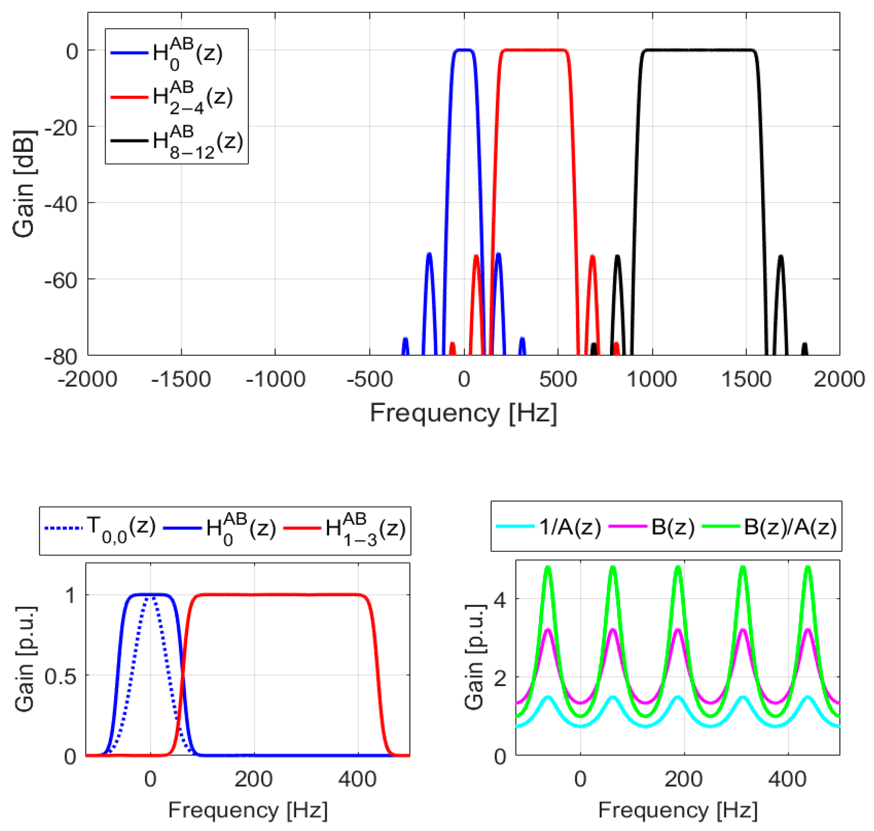
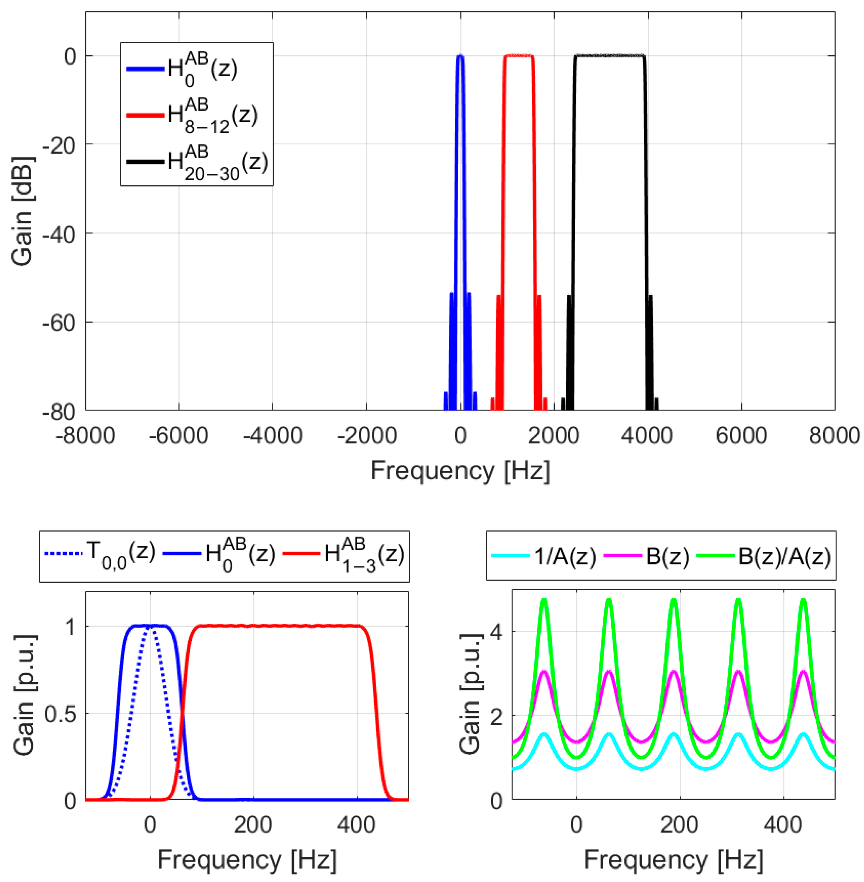
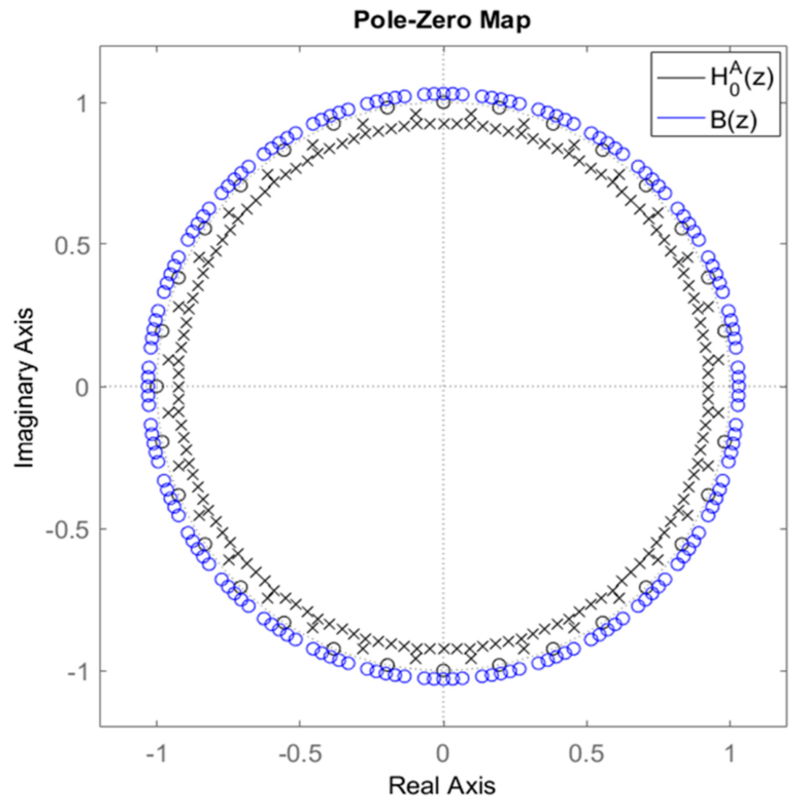
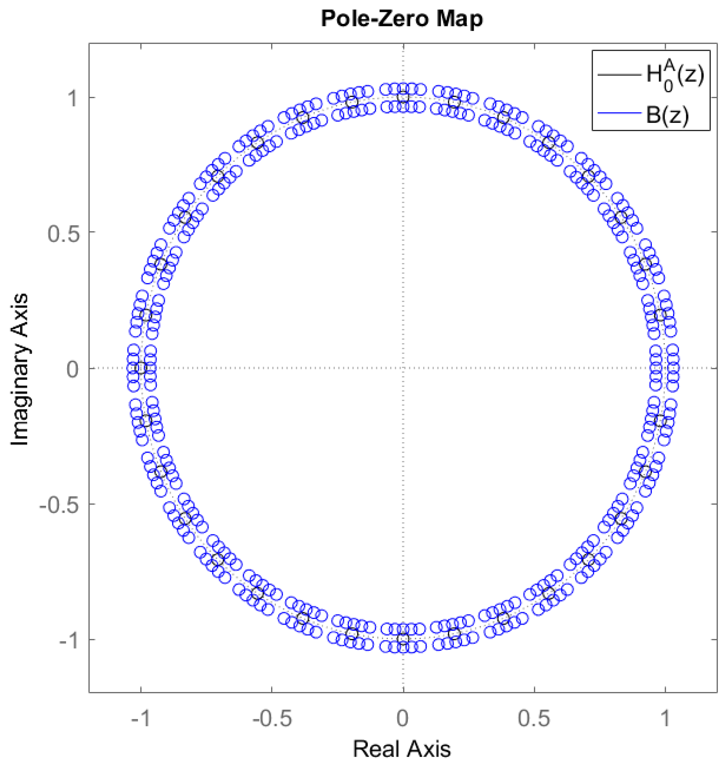
The first example (Figure 2) presents a $K=4$ type IIR CR-based filter bank, with $f_S=4 \mathrm{k}\mathrm{H}\mathrm{z}$, $f_1=125 \mathrm{H}\mathrm{z}$, and $M=15$. The parameters are set as $N_A=N_B=\left(K+1\right)\left(2M+2\right)$ and ${\tau }_B=N_B$. It is worth nothing that the ripples in the passband are minimal, with the maximum value of 0.02 dB. Figure 3 displays pole-zero maps of the transfer functions $H\left(z\right)$, $A\left(z\right),$ and $B\left(z\right)$. The diagram clearly shows full periodicity, with the pole-zero-maps for other harmonic components able to be obtained by rotating this one. Note that for the harmonic $m=0$ (DC component), zeros around the pole $z=1$ (corresponding to frequency 0 Hz) are absent, whereas for the other harmonics, they are present with multiplicity of 5 ($\mathrm{t}\mathrm{h}\mathrm{a}\mathrm{t}\mathrm{i}\mathrm{s}\mathrm{e}\mathrm{q}\mathrm{u}\mathrm{a}\mathrm{l}\mathrm{t}\mathrm{o} K+1$). Additionally, simulations indicate that setting $N_A^R=2$, i.e., $N_A=2\left(2M+2\right)$, is sufficient, as further increases do not yield significant improvements in design performance. Indeed, reducing $N_A$ does not reduce the computational burden during implementation; however, it decreases the number of optimization parameters, thereby shortening the design time. Unlike $N_A$, increasing $N_B$ has a significant impact on performance improvement, particularly in reducing ripple in the passband. However, the downside is an increase in group delay ${\tau }_B$.

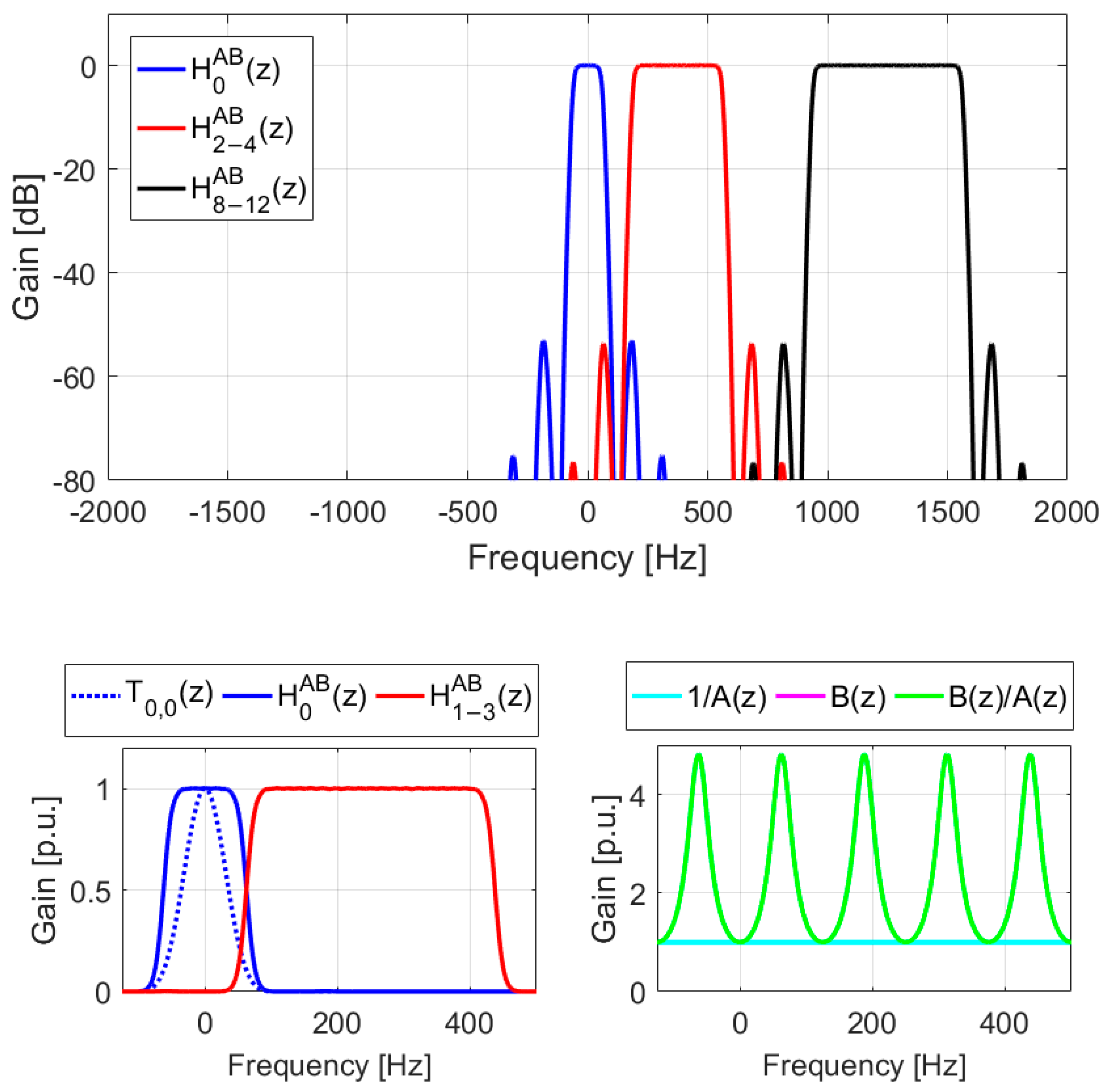
Figure 4 and Figure 5 show the results obtained for the case of FIR transfer functions. The parameters were set to $N_A=0$, $N_B=2\left(K+1\right)\left(2M+2\right)$ $\mathrm{a}\mathrm{n}\mathrm{d}{\tau }_B=N_B/2$, while all other parameters remained the same as in the previous case. Note that the required group delays are identical in both cases, ${\tau }_B=\left(K+1\right)\left(2M+2\right)$.

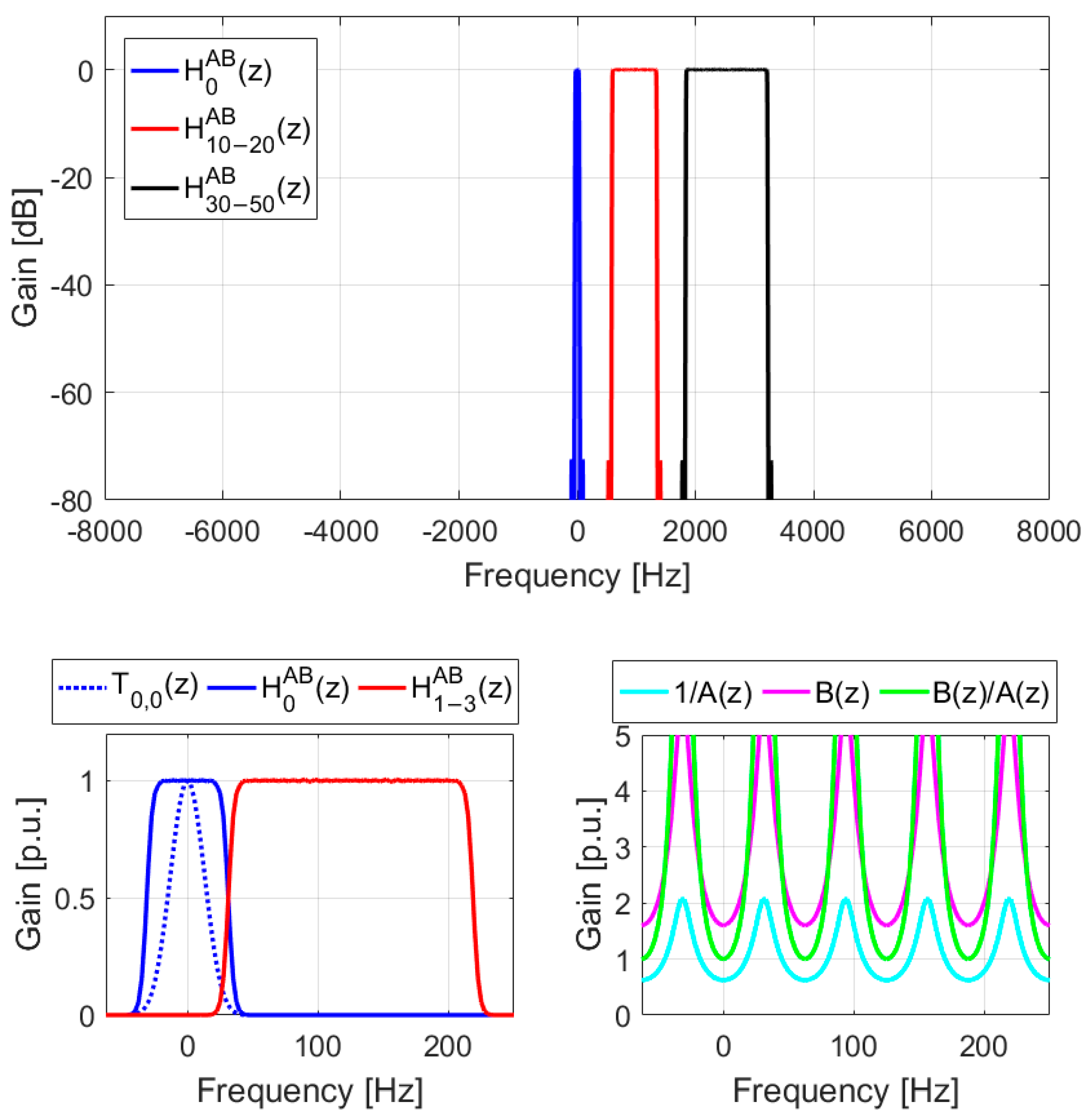
Figure 6 shows the frequency characteristics of the filter bank obtained under the same conditions as in the previous example, but with a higher sampling frequency of $f_S=16 \mathrm{k}\mathrm{H}\mathrm{z}$. This enables a broader frequency range up to $f=\pm 8 \mathrm{k}\mathrm{H}\mathrm{z}$, or 64 frequency bands with a bandwidth of 125 Hz per band.

In the last example (Figure 7), with $K=6,$ $f_S=16 \mathrm{k}\mathrm{H}\mathrm{z}$, $f_1=62.5 \mathrm{H}\mathrm{z}$, and $M=127$, both $N_A$ and $N_B$ are selected as $\left(K+1\right)\left(2M+2\right),$ and ${\tau }_B=N_B$. The maximum ripple in the passband is 0.02 dB. In this case, due to higher value of $K$, the impact of the sidelobes of harmonic filters in the primary filter bank is negligible. The frequency responses of the filters $A\left(z\right)$ and $B\left(z\right)$, shown in the inset figures at the bottom of the main figure, exhibit higher amplitudes compared to when $K=4$. Additionally, it is evident that the analyzers with a higher number of resonators result in lower sidelobes and improved sharpness.

The passband widths can be easily adjusted in real time by modifying the number of adjacent output signals from the CR structure. The frequency responses indicate that as $K$ increases, the amplitudes of the frequency responses in the compensation part also rise. This leads to an increase in the primary sidelobes in the stopbands of the filters in the desired filter banks when compared to the basic bank filters. The magnitude of this increase in sidelobes corresponds to the magnitude of the frequency response of the transfer function $B\left(z\right)/A\left(z\right)$.

The height of the lateral lobes depends on the value of $K$, with the relationship between these two parameters shown in

Table 1. Sidelobe levels as functions of $K$.

$\mathit{K}$	Sidelobe Level
1	−20 dB
2	−35 dB
3	−43 dB
4	−55 dB
5	−63 dB
6	−73 dB

. Sidelobe levels can be reduced by introducing constraints into the optimization process; however, this may compromise the flatness of the passband. It should also be noted that the optimization errors are influenced by the chosen value of ${\tau }_B$, which is selected heuristically. Additionally, ${\tau }_B$ affects the amplitude ratio between the frequency responses $A\left(z\right)$ and $B\left(z\right)$.

5. Conclusions

Considering the periodicity of the frequency responses, this paper presented significant advancements in the design and optimization of cascaded-resonator (CR)-based filter banks, focusing on improving computational efficiency and adaptability for real-time signal analysis. By introducing modifications to the characteristic polynomial modeling and employing quadratic programming optimization, the proposed method achieves faster, more robust filter bank designs, even in complex systems. These improvements enhance the applicability of CR-based filter banks in various fields, such as speech analysis, hearing correction, and dynamic spectrum management. Future work could explore further optimization strategies and their real-world implementations in communication systems.

A key advantage of this approach is its ability to dynamically adjust the bandwidths of filters in real time. This is accomplished through the simple inclusion or exclusion of output signals from adjacent channels within the basic filter bank. Moreover, the selectivity can be increased to any desired level. However, the main drawback of this method is its relatively high computational complexity, which may be a limiting factor in cost-sensitive or low-power applications.