Classification-Based Q-Value Estimation for Continuous Actor-Critic Reinforcement Learning

Abstract

Stable Q-value estimation is critical for effective policy learning in deep reinforcement learning (DRL), especially continuous control tasks. Traditional algorithms like Soft Actor-Critic (SAC) and Twin Delayed Deep Deterministic (TD3) policy gradients rely on Mean Squared Error (MSE) loss for Q-value approximation, which may cause instability due to misestimation and overestimation biases. Although distributional reinforcement learning (RL) algorithms like C51 have improved robustness in discrete action spaces, their application to continuous control remains computationally expensive owing to distribution projection needs. To address this, we propose a classification-based Q-value learning method that reformulates Q-value estimation as a classification problem rather than a regression task. Replacing MSE loss with cross-entropy (CE) and Kullback–Leibler (KL) divergence losses, the proposed method improves learning stability and mitigates overestimation errors. Our statistical analysis across 30 independent runs shows that the approach achieves an approximately 10% lower Q-value estimation error in the pendulum environment and a 40–60% reduced training time compared to SAC and Continuous Twin Delayed Distributed Deep Deterministic (CTD4) Policy Gradient. Experimental results on OpenAI Gym benchmark environments demonstrate that our approach, with up to 77% fewer parameters, outperforms the SAC and CTD4 policy gradients regarding training stability and convergence speed, while maintaining a competitive final policy performance.

1. Introduction

Reinforcement learning (RL) [1] has emerged as a powerful framework for solving complex sequential decision-making problems, including robotic control [2], game playing [3], and autonomous driving [4]. In RL, the balance between exploration and exploitation reflects a fundamental symmetry, as the learning process strives to optimize both stability and adaptability in dynamic environments [1,2,3,4]. The success and applicability of RL algorithms depend critically on the accurate and stable estimation of action-value functions (Q-values), which directly influence the quality of learned policies. Prominent continuous control algorithms, such as Soft Actor-Critic (SAC) [5] and Twin Delayed Deep Deterministic (TD3) policy gradients [6], estimate Q-values through regression using Mean Squared Error (MSE) loss functions. However, MSE-based Q-value estimation often suffers from instability during training, leading to issues such as the overestimation and underestimation of Q-values, which can negatively affect policy optimization [7].

To address these limitations, distributional RL [8], which offers an alternative approach by modeling Q values as probability distributions rather than scalar values, has been proposed. Algorithms such as C51 [8,9] and the Quantile Regression Deep Q-Network (QR-DQN) [10] improve learning stability by estimating the full distribution of Q-values. Specifically, C51 represents the Q-value distribution using a fixed number of discrete bins (e.g., 51 atoms) and minimizes the Kullback–Leibler (KL) divergence between the predicted and target distributions [11]. Although C51 employs a projection step to convert the KL loss into a cross-entropy (CE) loss for computational efficiency, this approach introduces additional complexity. Moreover, distributional methods, such as C51, are primarily designed for discrete action spaces, and their direct application to continuous control environments poses significant computational challenges owing to the need for distribution projection operations.

Actor-Critic architectures have been widely adopted in continuous control RL [12]. In this framework, the Critic estimates the Q-values for state–action pairs, whereas the Actor optimizes the policy based on the Critic’s feedback. The application of distributional RL to continuous action spaces presents unique challenges. First, because Q-values are represented as distributions rather than scalars, the Actor requires additional approximation steps to transform discrete Q-value distributions into continuous actions, thereby increasing the computational overhead. Second, while algorithms such as TD3 and SAC achieve efficient Q-value estimation through regression, incorporating distributional methods significantly increases training costs, hindering real-time decision making. Consequently, directly integrating distributional RL, such as C51, into continuous Actor-Critic frameworks is impractical owing to the computational burden associated with distribution projections and policy updates.

To overcome these challenges, this paper introduces a novel approach that leverages the classification-based Q-value estimation method proposed in the Stop Regressing framework [13] and applies it to continuous control environments. Traditional RL methods deal with Q-value estimation as a regression problem optimized using MSE loss. In contrast, this approach reconceptualizes Q-value estimation as a classification problem by segmenting Q-values into discrete intervals to enable predictions through classification models. This shift from regression to classification enhances learning stability and efficiency. Specifically, the proposed method integrates a classification-based Q-value learning method directly into the Actor-Critic architecture for continuous action spaces, providing a computationally efficient and robust alternative to conventional distributional RL methods.

The key contributions of this research are as follows:

• Computational and Learning Efficiency: Our classification-based approach reduces computational overhead by eliminating the complex distribution projection operations required in distributional RL methods, such as C51, while enhancing learning stability by replacing MSE loss with CE loss and KL divergence loss. This dual enhancement enables faster learning convergence with a significantly reduced training time (40–60% reduction across environments) and improved Q-value estimation accuracy (approximately 10% lower error in an environment).
• Improved Training Robustness with Q-Value Lower Bounds: Inspired by techniques from previous studies [14], the proposed method applies Q-value lower bounds during training to further enhance stability. This prevents Critics from predicting abnormally low Q-values, which could negatively influence the Actor’s policy updates, resulting in a substantially reduced loss volatility (approximately 90% reduction in loss fluctuations) compared to existing methods.
• Seamless Integration into Actor-Critic Frameworks: Our approach integrates into continuous Actor-Critic architectures with minimal structural changes—modifying only the Critic’s output layer to produce a distribution over Q-value bins instead of a scalar Q-value, while preserving the Actor’s original structure and the standard policy gradient optimization mechanism. This simplicity ensures a broad applicability across various reinforcement learning scenarios without requiring a fundamental algorithm redesign.

The primary novelty of the proposed method is that it is one of the first to apply classification-based Q-value estimation to continuous control RL environments. While the Stop Regressing framework [13] was originally designed for discrete action spaces, we extend its applicability to continuous domains by integrating it into an Actor-Critic architecture. Additionally, we demonstrate that replacing MSE loss with CE loss and KL divergence loss improves both learning performance and stability. Furthermore, we introduce Q-value lower bounds to prevent negative-value drift during training, ensuring a more reliable policy optimization.

Our approach is particularly relevant for resource-constrained applications, such as IoT devices and edge computing, where Fan et al. [15] demonstrated the value of computationally efficient reinforcement learning for secure information systems. Our method’s substantial parameter count reduction (up to 77% fewer parameters) compared to other methods makes it well-suited for such deployment scenarios. Its enhanced stability and reduced computational requirements enable real-time decision making in embedded systems and mobile robotics, where processing power and memory are limited but reliable performance is essential.

To validate the effectiveness of the proposed method, extensive experiments were conducted in various continuous control environments using the OpenAI Gym platform [16]. We compared this with the CTD4 Policy Gradient [17], which adapts distributional RL concepts for continuous spaces, and the well-established SAC algorithm. Statistical analysis across 30 independent runs demonstrated that the proposed method achieved a superior performance in terms of learning stability and convergence speed, with up to two-fold faster convergence in complex environments, highlighting its potential as a robust alternative to traditional regression-based Q-value estimation methods in continuous RL settings.

2. Related Works

The accurate estimation of action-value functions (Q-values) is crucial for maintaining policy stability in RL environments because it significantly affects both learning robustness and the efficiency of policy optimization [17,18,19]. Well-known RL algorithms such as SAC [5] and the TD3 policy gradient [6] learn Q-values using the MSE loss function. However, MSE-based Q-value learning can lead to over- and underestimation, which can potentially cause training instability [7]. To address these challenges, distributional-based and classification-based RL approaches have been proposed. These algorithms improve learning stability by modeling Q-values as probability distributions [8,9] or classification techniques [13]. This section reviews key studies related to distributional RL, the Stop Regressing approach, and the CTD4 policy gradient algorithm, highlighting their relevance to our proposed method.

2.1. Distributional Reinforcement Learning

Traditional Q-learning relies on the Bellman Expectation Equation to update Q-values.

$$Q^{*}\left(s,a\right)=\mathbb{E}\left[r+\gamma {max}_{a^{\prime }}{Q}^{*}\left(s^{\prime },a^{\prime }\right)|s,a\right]$$

(1)

where $Q^{*}\left(s,a\right)$ represents the optimal Q-value for state $s$ and action $a$, $r$ is the reward, $\gamma$ is the discount factor, $s^{\prime }$ is the next state, and $a^{\prime }$ is the next action. This approach models Q-values as single scalar expectations that fail to capture uncertainty during learning, leading to instability. To overcome this problem, distributional RL methods such as C51 [8,9] and QR-DQN [10] have been introduced. These algorithms model Q-values as probability distributions rather than scalars, thereby enhancing the prediction accuracy. The distributional version of the Bellman equation is defined as follows:

$$Z\left(s,a\right)=D\left[r+\gamma Z(s^{\prime },a^{\prime })\right]$$

(2)

where $Z\left(s,a\right)$ represents the random return from taking action $a$ in state $s$ and $D$ denotes the distributional Bellman operator [8,9]. C51 represents Q-values using discrete probability distributions with a fixed number of “atoms”, assigning probability masses to each state–action pair. However, applying C51 in continuous action spaces requires additional categorical projection steps, which increases computational costs [13]. Therefore, there is a growing need for efficient Q-value learning techniques that are suitable for continuous environments.

2.2. Stop Regressing: Classification-Based Q-Value Learning

In conventional RL algorithms, Q-values are typically learned using MSE loss, as follows:

$$L_{MSE}=\mathbb{E}\left[{\left(Q_{\theta }\left(s,a\right)-y\right)}^2\right]$$

(3)

where $Q_{\theta }\left(s,a\right)$ is the predicted Q-value with the parameter $\theta$ and $y$ is the target Q-value [1]. This regression-based approach often suffers from overestimation and underestimation, leading to unstable learning [13].

The Stop Regressing method [13] addresses this by framing Q-value estimation as a classification problem. It discretizes Q-values into categorical labels and predicts the probability of each class using classification techniques. This approach employs CE loss and KL divergence loss functions to enhance learning stability, as follows:

$$L_{CE}=-{\sum }_{i=1}^N{p}_i\log \widehat{p_i}$$

(4)

$$L_{KL}= {\sum }_{i=1}^N{p}_i\log {\displaystyle \frac{p_i}{\widehat{p_i}}}$$

(5)

where $p_i$ is the target probability distribution, $\widehat{p_i}$ is the predicted probability distribution, and $N$ is the number of classes.

Various probabilistic loss functions offer different theoretical properties for reinforcement learning. According to Rowland et al. [20], KL divergence is sensitive to differences in the probability mass between distributions, whereas Wasserstein distance is more sensitive to changes in the distribution shape. Hellinger distance exhibits intermediate characteristics between the two metrics. However, as Müller et al. [21] noted, Wasserstein distance requires solving an optimal transport problem, which introduces considerable computational complexity. The Wasserstein distance between the two distributions $p$ and $q$ is defined as follows:

$$L_W={inf}_{\gamma \in \Gamma (p,q)}{E}_{\left(x,y\right)~\gamma }\left[\parallel x-y\parallel \right]$$

(6)

where $\Gamma (p,q)$ is the set of all joint distributions with marginals $p$ and $q$. Hellinger distance, which offers a middle ground between KL divergence and Wasserstein distance, is defined as follows:

$$L_H={\sum }_{i=1}^K{\left(\sqrt{p_i}-\sqrt{q_i}\right)}^2$$

(7)

Although these alternative metrics offer theoretical benefits in capturing distribution characteristics, computational considerations in practical implementations remain significant, particularly for real-time applications and resource-constrained environments.

2.3. Binning Strategies in Distributional Reinforcement Learning

Binning strategy selection is a critical design decision in distributional and classification-based Q-value learning. Bellemare et al. [8] employed uniform binning in their original work, whereas subsequent studies explored adaptive strategies such as quantile-based binning [10]. According to Doya et al. [18], uniform discretization exhibits asymptotic optimality for consistent target distributions from a KL divergence minimization perspective. This theoretical foundation supports the use of fixed binning strategies in many applications.

Fixed binning offers several advantages. First, a deterministic upper bound on computational complexity $(O\left(K\right))$ is ensured at each training step, where $K$ denotes the number of bins. Second, fixed binning has a mathematically proven compatibility with the Bellman operator [8], providing theoretical guarantees for convergence. Third, it requires no separate parameterization of bin boundaries, which reduces memory requirements and model complexity. These benefits make fixed binning particularly suitable for real-time online reinforcement learning applications.

However, adaptive binning strategies, such as quantile-based binning, can potentially offer improvements in environments with nonuniform reward distributions. Adaptive approaches dynamically adjust bin boundaries to better capture the underlying distribution of Q-values, which can theoretically improve representational accuracy. This creates an interesting trade-off between computational efficiency and distributional expressiveness, which warrants further investigation in future research.

2.4. CTD4 Policy Gradient: Continuous Distributional Actor-Critic Algorithm

The CTD4 Policy Gradient integrates distributional Q-value estimation with Actor-Critic architectures, extending the traditional TD3 and SAC frameworks [17]. The CTD4 Policy Gradient models Q-values using Gaussian distributions and employs Kalman-filter-based Critic fusion to enhance prediction accuracy, as follows:

$$Q_{\theta }(s,a)~\mathcal{N}\left({\mu }_{\theta }\left(s,a\right),{\sigma }_{\theta }(s,a)\right)$$

(8)

where ${\mu }_{\theta }\left(s,a\right)$ is the mean and ${\sigma }_{\theta }(s,a)$ is the standard deviation of the predicted Q-value distribution. The Gaussian modeling approach in the CTD4 Policy Gradient offers advantages in continuous spaces but introduces limitations when Q-value distributions exhibit non-Gaussian characteristics. Additionally, the Kalman filter fusion mechanism, while theoretically sound for combining multiple estimates, can be susceptible to instability in complex environments with unexpected transitions.

Although the CTD4 Policy Gradient improves learning stability through Gaussian-based estimation and Critic fusion, it remains fundamentally dependent on MSE loss and does not fully eliminate training instability. Furthermore, the additional computational requirements of Gaussian modeling and Kalman fusion present challenges for their deployment in resource-constrained environments.

2.5. Practical Applications of Reinforcement Learning and Computational Efficiency

Recently, reinforcement learning has expanded beyond robot control and game agents to various real-world applications. Applications in resource-constrained environments are particularly gaining attention, and Fan et al. [15] proposed a reinforcement-learning-based approach for secure information systems in smart cities. Their research demonstrated that combining deep reinforcement learning with blockchain in collaborative IoT computing could simultaneously enhance computational efficiency and security.

In such resource-constrained contexts, both computational efficiency and algorithmic stability become critical considerations. Kumar et al. [19] emphasized the importance of efficient reinforcement learning in these environments, improving sample efficiency through representation learning. Zhao and Xu [14] demonstrated that setting Q-value lower bounds can enhance the stability in these scenarios, preventing value estimates from diverging during training.

Hessel et al. [22] demonstrated the importance of combining various improvements in deep reinforcement learning, including distributional approaches, but they did not explicitly compare the computational efficiencies of the different methods. This research gap motivated the current study, which focuses on both performance and computational efficiency, particularly for continuous control tasks in potentially resource-constrained environments.

As the practical applications of reinforcement learning continue to expand into domains such as edge computing, IoT devices, and embedded systems, the importance of computationally efficient and stable Q-value estimation methods has become increasingly significant. This trend emphasizes the need for algorithms that can maintain a robust performance while minimizing computational overhead, a balance our proposed method aims to achieve.

3. Proposed Method

3.1. Research Objectives and Approach

This paper proposes a novel classification-based Q-value estimation method to address the limitations of traditional MSE-based Q-value learning. By applying the classification technique introduced in the Stop Regressing framework to continuous RL environments, we intend to enhance learning stability and improve performance.

The core achievements of this study are as follows:

• Reformulating Q-Learning as a Direct Classification Problem: While C51 employs binning within a distributional RL framework requiring complex Bellman projection operations, our approach directly frames the entire Q-value estimation as a classification task without distributional Bellman updates. This fundamental shift eliminates the computationally expensive projection step required in C51 and allows for the direct application of classification losses (CE/KL divergence) to Q-value learning, simultaneously achieving conceptual simplicity and computational efficiency.
• Improved Training Robustness with Q-Value Lower Bounds: Inspired by techniques from previous studies [14], the proposed method applies Q-value lower bounds during training to further enhance stability. This prevents Critics from predicting abnormally low Q-values, which could negatively influence the Actor’s policy updates, resulting in a substantially reduced loss volatility compared to competing methods.
• Seamless Integration into Actor-Critic Frameworks: Our approach integrates into continuous Actor-Critic architectures with minimal structural changes—modifying only the Critic’s output layer to produce a distribution over Q-value bins instead of a scalar Q-value, while preserving the Actor’s original structure and the standard policy gradient optimization mechanism.

Our approach maintains the traditional Actor-Critic framework but introduces a fundamental shift in the Critic’s Q-value learning process, moving from regression- to classification-based learning. While the CTD4 Policy Gradient models Q-values using Gaussian distributions to predict the mean (μ) and standard deviation (σ), our method discretizes Q-values into specific intervals (bins) and predicts their probabilities through classification. This transformation aims to reduce Q-value estimation uncertainty and enhance learning stability.

3.2. Key Differences from CTD4 Policy Gradient

The CTD4 Policy Gradient employs Gaussian-based Q-value modeling with Kalman Fusion to aggregate outputs from multiple Critics, thereby improving the learning stability. However, this introduces additional computational costs and retains MSE-based loss functions, which can lead to learning instability. To address these issues, our method introduces classification-based Q-value estimation with the following distinctions: The major differences between our approach and existing methods such as CTD4 and C51 are summarized in

Table 1. Key Differences from CTD4.

Aspect	CTD4 (Existing Method)	Proposed Method (This Study)
Q-Value Modeling	Gaussian Distribution	Discrete Binned Distribution (Classification-Based)
Loss Function	Mean Squared Error (MSE)	Cross-Entropy (CE)/Kullback–Leibler (KL) Divergence
Critic Architecture	Gaussian Mean Prediction	Classification-Based Q-Value Estimation
Learning Stability	Underestimation of Overestimation based on MSE	Improved Stability through Classification
Computational Efficiency	Modeling with Kalman Fusion	Simplified Single-Critic Architecture

.

• Unlike traditional classification tasks, the proposed approach does not rely on explicit labels. Instead, it discretizes Q-values into bins without directly modeling the probability distributions, as in distributional RL algorithms such as C51.
• Although C51 explicitly learns probability distributions, our method predicts Q-values using a bin-based estimation strategy without projection operations.

As illustrated in Figure 1, we replace the Gaussian-based Q-value learning mechanism with a bin-based classification approach. This modification eliminates the need for Gaussian modeling while maintaining learning stability without relying on Kalman Fusion.

3.3. Proposed Q-Value Learning Method

• The Discretization of Q-Values and Application of the Stop Regression Method: In contrast to traditional MSE-based Q-value learning, which predicts continuous scalar values, the proposed method transforms Q-values into discrete intervals (bins) and addresses the problem as a classification task. This reduces estimation uncertainty and enhances training stability.
• The Incorporation of CE and KL Divergence Loss Functions: MSE loss often causes sharp fluctuations and divergence issues during training. To address this, we apply the CE and KL divergence loss functions, which provide smoother gradient updates and an improved stability.
• Simplified Single-Critic Architecture (Without Kalman Fusion): Although the CTD4 policy gradient utilizes multiple Critics with Kalman Fusion to aggregate Q-values, our method adopts a single-critic structure, significantly reducing computational costs while maintaining a comparable performance. This design improves training speed without compromising learning efficiency.

3.4. Application in the Actor-Critic Framework

3.4.1. Actor’s Role

The Actor receives the current state s and selects an optimal action a based on the stochastic policy ${\pi }_{\theta }$ [12], as follows:

$${\pi }_{\theta }(a|s)$$

(9)

Unlike Gaussian-based methods, in which the Actor samples continuous actions evaluated by the Critic, our classification-based Critic provides more stable Q-value feedback, facilitating robust Actor updates.

3.4.2. Critic’s Role

The Critic transforms continuous Q-values into discrete bins and predicts the probability of each bin using classification techniques. The training process involves two key steps.

• Bellman Update: Target Q-values are converted into discrete bins.
• Probability Prediction: The likelihood of each bin is estimated and optimized using the CE or KL divergence loss functions.

These improvements stabilize Actor updates and enhance overall policy performance.

3.5. Mathematical Formulation of Q-Value Learning

3.5.1. Modeling Q-Values as Discrete Distributions

Traditional Q-learning relies on the Bellman Expectation Equation [1], as follows:

$$Q\left(s,a\right)\leftarrow r+\gamma {max}_{a^{\prime }}Q\left(s^{\prime },a^{\prime }\right)$$

(10)

where $Q\left(s,a\right)$ represents the action-value function for state $s$ and action $a$, $r$ is the immediate reward received after taking action $a$ in state $s$, $\gamma$ is the discount factor that determines the importance of future rewards, $s^{\prime }$ is the next state, and $a^{\prime }$ is the next action. The ${max}_{a^{\prime }}Q\left(s^{\prime },a^{\prime }\right)$ selects the maximum Q-value achievable from the next state by choosing the optimal action.

In contrast, our method discretizes Q-values into K bins, modeling the distribution as follows:

$$P\left(Q\right)=\left\{p_1, p_2,\cdots ,p_k\right\}, {\sum }_{i=1}^K{p}_i=1$$

(11)

where $K$ represents the number of bins and $p_k$ denotes the probability of the Q-value falling into bin $k$. The conversion from continuous Q values to bins follows the deterministic mapping function. For any Q-value $q$ within the range $[V_{min}, V_{max}]$ in the proposed algorithm, the corresponding bin index $i$ is computed as follows:

$$i=\left[{\displaystyle \frac{q-V\_min}{V_{max}-V_{min}}}\right]·K$$

(12)

This equation maps any Q-value to its appropriate bin index, ensuring that the values are properly distributed across a defined range. During training, we apply a softmax activation function to the Critic’s output logits to obtain a proper probability distribution over the $K$ bins, as follows:

$$p_{i }={\displaystyle \frac{e^{z_i}}{\sum _{j=1}^K{e}^{z_j}}}$$

(13)

where $z_i$ represents the logit output for bin $i$ from the Critic network.

3.5.2. Policy Gradient for Classification-Based Q-Value Estimation

For policy optimization, we employ a classification-based variant of the deterministic policy gradient. Although the Actor network structure remains unchanged from traditional Actor-Critic methods, the gradient computation incorporates our classification-based Q-value estimates, as follows:

$${\nabla }_{\theta }J\left(\theta \right)=E_{s~p^{\pi }}\left[{\nabla }_{\theta }{\pi }_{\theta }(s){\nabla }_{a}Q(s,a){\sum }_{i=1}^K{p}_i{v}_i\right]$$

(14)

where $p_i(s,a)$ represents the probability of a Q-value falling into bin $i$ and $v_i$ is the center value of bin $i$. The term $\sum _{i=1}^K{p}_i{v}_i$ corresponds to the expected Q value under the predicted distribution.

The expected Q-value used for actor updates is calculated as follows:

$${\rm E}\left[Q(s,a)\right]={\sum }_{i=q}^K{p}_i{v}_i$$

(15)

The center value $v_i$ for each bin is defined as follows:

$$v_i=V_{min}+{\displaystyle \frac{\left(i-0.5\right)}{K}}·(V_{max}-V_{min})$$

(16)

This formulation enables a smooth and differentiable computation of the expected Q-value from a probability distribution, which is essential for stable policy gradient updates. Unlike traditional scalar Q-value approaches, this method captures the uncertainty in value estimation through a distributional representation.

3.5.3. Rationale for Loss Function Selection

• Theoretical Advantages of CE and KL Loss Functions

The CE and KL divergence loss functions offer several theoretical advantages for Q-value estimation compared to traditional MSE loss, as follows:

• Gradient Stability: The CE and KL divergence loss functions provide more stable gradients when learning probability distributions. Unlike MSE, which can produce extreme gradients for outlier values, these probabilistic losses naturally bind the gradient magnitudes, resulting in more stable learning trajectories.
• Probabilistic Distribution Expressiveness: These losses are specifically designed to compare probability distributions, making them naturally suited for our classification-based approach, where Q-values are represented as distributions over discrete bins.
• Robustness to Outliers: Unlike MSE, which heavily penalizes large errors (because of its squared term), the CE and KL divergence loss functions are more robust to occasional extreme values or noise in the target Q-values.

• Comparative Analysis with Alternative Loss Functions

We considered the Hellinger distance and Wasserstein distance as alternatives, but selected CE and KL divergence for the following reasons:

• Computational Efficiency: Wasserstein distance requires solving an optimal transport problem with a computational complexity of $O(n^{2}log(n))$ in the worst case, adding approximately $37\%$ additional computational overhead to training. Hellinger distance, while less intensive, still introduces approximately $20\%$ overhead compared with CE/KL divergence implementations.
• Implementation Complexity: The Wasserstein and Hellinger distances require additional projection operations and more complex gradient calculations, which could significantly increase the implementation complexity without proportional performance benefits.
• Training Stability: From a theoretical perspective, the CE/KL divergence losses provide an excellent stability in classification problems. CE loss is particularly effective in preventing the model from becoming overconfident in its predictions, whereas KL divergence ensures that the predicted distribution matches the target distribution.

• Justification for Loss Function Selection

The CE and KL divergence loss functions provide an optimal balance between the theoretical properties and practical implementation.

• They maintain mathematical compatibility with the Bellman operator in RL.
• They offer a superior computational efficiency compared to Wasserstein metrics.
• They demonstrate excellent theoretical properties for learning stability.
• They are well-suited for optimization in deep neural network architectures.

Therefore, the CE and KL divergence loss functions are more suitable choices for Q-value learning than the Wasserstein or Hellinger distances, which offer limited theoretical advantages relative to their increased computational complexity.

3.5.4. Binning Strategies: Fixed Binning vs. Quantile Binning

• Fixed Binning: Divides the Q-value range into equal intervals (e.g., discretizing Q-values from [−10, 10] into 51 bins, as in C51 [8,9]).
• Quantile Binning: Bin boundaries are adjusted based on the data distribution to ensure equal probability mass across bins.

We adopt Fixed Binding for computational efficiency while ensuring a balanced bin distribution during training. Our implementation uses 51 bins following the original C51 architecture, which provides a sufficient resolution for accurate Q-value representation while maintaining computational efficiency. The bin boundaries are defined as follows:

$$b_j=V_{min}+j·∆, for j\in \left\{\mathrm{0,1},\dots ,K\right\}$$

(17)

where $∆={\displaystyle \frac{V_{max}-V_{min}}{K}}$ is the width of each bin.

The bin boundaries remain fixed throughout the training, which contributes to the stability of the learning process. To determine the appropriate values of $V_{min}$ and $V_{max}$, we conduct preliminary experiments for each environment and select ranges that cover the expected distribution of the Q-values.

• Our fixed binning approach offers several key technical advantages, as follows:

• Deterministic Upper Bound on Computational Complexity: Fixed binning guarantees a consistent computational complexity $O(K)$ at each training step (where $K$ is the number of bins). This provides predictable performance characteristics during both training and inference. By contrast, adaptive binning requires an additional $O(N log N)$ computation (where $N$ is the batch size) for bin boundary readjustment, potentially creating computational bottlenecks.
• Gradient Stability and Convergence Guarantees: Fixed binning has a mathematically proven compatibility with the Bellman operator [8,9], which provides strong theoretical guarantees for convergence. Adaptive binning risks introduce additional nonstationarity owing to dynamically changing target distributions, which could destabilize the learning process.
• Memory Efficiency: Fixed binning requires no separate parameterization of the bin boundaries, leading to reduced memory requirements and a simpler network architecture. Adaptive binning might require additional networks or parameters to learn environment-specific bin boundaries, thereby increasing model complexity.
• Distributional Theoretical Optimality: Uniform discretization exhibits an asymptotic optimality for consistent target distributions from a KL divergence minimization perspective [18]. This theoretical property suggests that fixed binning can adequately capture the underlying Q-value distribution when using appropriate loss functions such as KL divergence.

The following is the description of the proposed method, which is also presented in Algorithm 1.

Algorithm 1 Classification-Based Q-value Estimation for Continuous RL

## Inputs: - state_size: Dimensions of state space - action_size: Dimensions of action space - $num\_bins$: number of bins for Q-value discretization. - $V\_min$: Minimum Q-value range - $V\_max$: maximum Q-value range Gamma: Discount factors - Learning _rate: Learning rate batchsize: Batch size. num_episodes ($N$): the number of training episodes max_steps ($T$): maximum steps per episode. - loss_type: “ce” (Cross-Entropy) or “kl” (KL Divergence) ## Outputs: - Trained Actor network ${\pi }_{\theta }(a|s)$ - Trained Critic network $Q_{\phi }(s,a)$ Initialize Phase 1.$\mathrm{Initialize} \mathrm{Actor} \mathrm{network} {\pi }_{\theta }\left(a|s\right)$ 2. Initialize classification-based Critic network $Q_{\varnothing }(s,a) (\mathrm{output}: \mathrm{logits} \mathrm{for} \mathrm{each} \mathrm{bin})$ 3.$\mathrm{Initialize} \mathrm{replay} \mathrm{buffer} B$ 4.$\mathrm{Calculate} \mathrm{bin} \mathrm{boundaries}: delta\_z=(V\_max-V\_min) / (num\_bins-1)$ 5.$\mathrm{Set} \mathrm{bin} \mathrm{center} \mathrm{values}: \{z\_i=V\_min+i \ast delta\_z for i in [0, 1, ..., num\_bins-1\left]\right\}$ Main Learning Loop for episode = 1 to $N$ do: Initialize environment and receive initial state $s$ Experience Collection for step = 1 to $T$do: Sample action from policy: $a ~ | {\pi }_{\theta }\left(a|s\right)$ Execute action $a$, receive reward $r$ and next state $s\prime$ Store experience $(s, a, r, s\prime , done)$ in replay buffer $B$ $s \leftarrow s\prime$ Terminate if done Batch Learning (if replay buffer $B$ has sufficient samples) Sample mini-batch $(s, a, r, s\prime , done)$ from $B$ Convert Q-values to classification targets (fixed binning) Predict next-state actions: $a\prime ={\pi }_{\theta }(s\prime )$ Calculate bin logits for next-state-action pairs: $logits\prime =Q_{\phi }(s\prime , a\prime )$ Calculate probabilities for next-state-action pairs: $P\prime =softmax(Q_{\phi }(s\prime , a\prime ) )$, $Q_{\phi }\left(s^{\prime }, a^{\prime }\right)\in R^K$ Calculate target Q-values: $z\_target=r+\gamma \ast z\_i \ast (1-done)$ Constrain $z\_target$ to $[V\_min, V\_max]$ range Project each target value to adjacent bins: - $b=(z\_target-V\_min) / delta\_z$ - $l=floor(b), u=ceil(b)$ - $P\_target\left[l\right]+=P\prime \ast (u-b)$ - $P\_target\left[u\right]+=P\prime \ast (b-l)$ Apply Cross-Entropy or KL Divergence loss Calculate logits for current state-action pairs: $logits=Q_{\phi }(s, a)$ Based on loss type: Cross-entropy: $L\_ce=-sum(P\_target \ast log(softmax(logits)))$ KL Divergence: $L\_kl=sum(P\_target \ast log(P\_target / softmax(logits)))$ Update Critic and Actor networks Update Qφ with Critic loss: - $\phi \leftarrow \phi -learning\_rate \ast \nabla \phi L (L is L\_ce or L\_kl)$ Calculate Actor loss: - Predict actions from current states: $a\_pred={\pi }_{\theta }(s)$ - Q-value of predicted actions: $Q\_pred=sum(softmax(Q_{\phi }(s, a\_pred)) \ast z\_i)$ - Actor loss: $L\_actor=-mean(Q\_pred)$ Update ${\pi }_{\theta }$ with Actor loss: −$\theta \leftarrow \theta -learning\_rate \ast \nabla \theta L\_acto$

3.6. Demonstrated Benefits of the Proposed Method

The proposed classification-based Q-value estimation offers significant improvements over the CTD4 Policy Gradient and SAC in terms of training stability, Q-value estimation accuracy, and computational efficiency, which will be empirically validated in the evaluation section.

3.6.1. Limitations of Gaussian-Based Q-Value Learning (CTD4 Policy Gradient)

• Noise Sensitivity: Gaussian models are theoretically more sensitive to noise in training data, which can lead to instability during policy optimization.
• Early Training Instability: Gaussian-based approaches may experience rapid Q-value fluctuations in the early training phases, potentially hindering convergence and optimal policy discovery.
• Limited Representation of Uncertainty: Gaussian distributions inherently make assumptions regarding the shape of the Q-value distribution, potentially oversimplifying the uncertainty representation and failing to capture complex multimodal Q-value distributions.

3.6.2. Core Innovations of the Proposed Method

• Transition from Regression to Classification: By discretizing the Q-values into bins, our approach reduces the adverse effects of function approximation errors and improves stability through a probabilistic representation.
• Use of CE and KL Divergence Loss Functions: These classification-oriented loss functions provide smoother gradient updates and an improved stability compared with MSE, potentially leading to faster convergence.
• Elimination of Projection (Compared to C51): Unlike C51, which requires complex projection operations in continuous spaces, our method directly applies classification without projection, thus reducing computational overhead without compromising performance.
• Simplified Critic (Without Kalman Fusion): Our single-Critic structure eliminates the need for the complex Kalman fusion techniques used in the CTD4 Policy Gradient, significantly reducing architectural complexity while maintaining robust Q-value estimation.

Our theoretical analysis suggests the following expected benefits:

• Enhanced Learning Stability. Our classification-based approach with CE/KL divergence loss functions theoretically provides more stable learning through the following:
  • Representing Q-values as discrete probability distributions rather than point estimates.
  • Using loss functions specifically designed for probability distributions.
  • Reducing sensitivity to outliers and extreme value estimations.
  • Providing more consistent gradient signals during training.
• Reduced Computational Overhead. The computational benefits of our approach stem from the following:
  • Eliminating the need for Kalman fusion operations required by the CTD4 Policy Gradient.
  • Removing the requirement for complex distribution projection operations.
  • Utilizing a simpler network architecture with fewer parameters.
  • Enabling more efficient forward and backward passes during training.
• Competitive Performance. Despite the simplifications, our method maintains strong theoretical properties, as follows:
  • Classification-based learning has strong theoretical guarantees for distribution estimation.
  • Probabilistic representation captures uncertainty in Q-value estimation.
  • Discretization reduces function approximation errors in complex value landscapes.
  • Fixed binning provides consistent learning targets across training iterations.

The theoretical advantages of our proposed method suggest improvements in both learning efficiency and performance stability, which are empirically validated in the following evaluation section. The proposed method was evaluated in various continuous action space environments, including LunarLanderContinuous-v2 [23], BipedalWalker-v3 [24], MountainCarContinuous-v0 [25], and Pendulum-v1 [26,27]. The experimental results demonstrate that our approach outperforms existing methods such as the SAC and CTD4 policy gradients in terms of training stability and convergence speed. These findings highlight the potential of the proposed classification-based Q-value estimation method to improve learning efficiency in RL, while effectively addressing the instability issues inherent in Gaussian-based Q-value estimation approaches.

4. Evaluation

In this section, we evaluate the proposed classification-based Q-value estimation method in comparison with existing RL algorithms, such as the CTD4 Policy Gradient and SAC. The evaluation focused on learning stability, Q-value prediction accuracy, and overall policy performance. Experiments were conducted in various continuous action-space environments provided by OpenAI Gym (v0.26.2), and the results were analyzed for each specific environment.

The decision to use a logarithmic (log) scale specifically for the BipedalWalker and LunarLander environments was driven by the unique characteristics and challenges associated with these tasks. Both environments are known for their highly complex and dynamic learning behaviors, which often result in extreme fluctuations in loss values during training. These fluctuations can span several orders of magnitude, making it challenging to accurately visualize and compare learning patterns on a linear scale.

In the BipedalWalker environment, the agent faces the challenge of maintaining balance while navigating uneven terrain, requiring the precise coordination of multiple joints. This results in highly unstable learning dynamics, particularly in the early stages of training, when the agent frequently loses balance or struggles to maintain effective locomotion. The corresponding Critic and Actor loss values can vary significantly, with sharp spikes and drops that are difficult to capture on a linear scale. Applying a log scale compresses these extreme variations, enabling a clearer visualization of both large fluctuations and subtle improvements in learning stability over time. Similarly, in the LunarLander environment, the agent must control multiple thrusters to achieve a smooth landing, balancing Actors such as velocity, angle, and fuel consumption. The learning process in this environment is extremely sensitive to slight changes in the policy of the agent, often leading to sudden and significant shifts in loss values. These abrupt changes, combined with outliers from failed landings, make it challenging to effectively interpret linear plots. The log scale mitigates this issue by reducing the visual impact of outliers while highlighting consistent learning trends, particularly in the later stages of training as the agent’s performance stabilizes. Furthermore, both environments require the agent to learn complex multidimensional policies, leading to oscillations in the loss functions as the agent explores and refines its strategies. The log scale is particularly effective for revealing these oscillations, making it easier to identify patterns of convergence and divergence that might otherwise remain hidden in a linear plot.

In contrast, simpler environments such as MountainCarContinuous and Pendulum exhibited more stable learning dynamics with less dramatic fluctuations in loss values, making linear scales sufficient for visualization. Therefore, the log scale was selectively applied to the BipedalWalker and LunarLander environments to better capture their complex learning behaviors, provide clearer insights into the training process, and facilitate a more accurate comparison of algorithm performance.

4.1. Pendulum-v1

The Pendulum-v1 environment is a simple continuous control task in which the agent learns to keep the pendulum upright by adjusting the torque. The reward function was designed to provide higher rewards as the pendulum approached the target position. The analysis of Figure 2 and Figure 3 is as follows.

• SAC exhibited large oscillations during early training and relatively slow convergence. This is attributed to the MSE-based Critic structure, which requires more time to stabilize the Q-value estimation.
• The CTD4 Policy Gradient, utilizing Gaussian-based Q-value predictions, converged faster than SAC and exhibited a reduced instability during the early learning phase.
• The proposed method demonstrated significantly faster convergence than both the SAC and CTD4 Policy Gradients. The Critic loss decreased sharply, indicating a higher learning stability.
• In terms of the policy performance, the proposed method achieved the highest final reward. This improvement is attributed to the CE and KL divergence loss functions, which effectively reduced Q-value uncertainty and facilitated faster policy optimization.

These results demonstrate that even in simple continuous control tasks, the proposed method effectively enhances the Q-value learning stability.

4.2. MountainCarContinuous-v0

The MountainCarContinuous-v0 environment challenges the agent to reach a goal by adjusting acceleration to overcome a steep hill. Owing to insufficient initial power, learning the optimal acceleration pattern is crucial. The analysis of Figure 4 and Figure 5 is as follows.

• SAC exhibited a slow learning progress and required considerable time to converge. This is likely because MSE-based Q-value learning struggles with fine-tuning, which is required for optimal policy learning.
• The CTD4 Policy Gradient showed faster learning than SAC, but some instability in the Q-values was observed during the early episodes, likely due to overestimation or underestimation by the Gaussian-based Critic structure.
• The proposed method’s use of CE and KL divergence loss enhanced learning stability by reducing the Q-value estimation variance and mitigating overfitting during training.
• Notably, from the mid-training phase onward, the proposed method demonstrated a significantly faster convergence rate, suggesting its superior ability to leverage reward signals compared with MSE-based approaches.

These results empirically verify that the proposed method enables faster and more stable learning of optimal policies in continuous-action environments.

4.3. LunarLanderContinuous-v2

The LunarLanderContinuous-v2 environment is a widely used benchmark in which the agent must learn to land a lunar module smoothly while conserving fuel. An agent is required to develop strategies for a controlled and efficient landing. The analysis of Figure 6 and Figure 7 is as follows.

• SAC exhibited significant fluctuations in rewards during the initial stages, along with slower convergence. Notably, Q-value instability led to frequent landing failures in some cases.
• The CTD4 Policy Gradient provided a more stable learning curve than SAC by leveraging its Gaussian-based Critic structure. However, large fluctuations in loss during the initial learning phase indicated persistent Q-value instability.
• The proposed method demonstrated rapid increases in rewards from the early training phase, achieving faster policy optimization than the other algorithms.
• The final rewards achieved by the proposed method were higher than those of both the SAC and CTD4 Policy Gradients, with a noticeably reduced volatility in the learning performance.
• Regarding Critic loss, the proposed method maintained the lowest and most stable values, with an increased stability as the training progressed.

These results confirm that the classification-based Q-value estimation approach ensures stable learning even in complex environments such as LunarLanderContinuous-v2. Furthermore, it empirically outperformed the SAC and CTD4 Gradients in terms of landing success rates and policy optimization speed.

4.4. BipedalWalker-v3

The BipedalWalker-v3 environment presents a complex, continuous control challenge that requires an agent to master bipedal walking while maintaining balance. Precise Q-value estimation is essential for learning effective walking strategies. The analysis of Figure 8 and Figure 9 is as follows.

• SAC demonstrated slow learning progression, with notable declines in rewards during certain training phases. This was likely due to the overestimation or underestimation of the Q-value, which disrupted consistent policy optimization.
• The CTD4 Policy Gradient exhibited a more stable learning curve than SAC, leveraging its Gaussian-based Critic structure. However, it still exhibited considerable fluctuations and struggled to maintain stable convergence in such a highly complex environment.
• The proposed method achieved steady reward growth from the early stages of training, showing the fastest policy convergence among all evaluated algorithms.
• In terms of Critic loss, the proposed method maintained the lowest and most stable values, indicating a well-balanced Q-value estimation.
• Notably, the final rewards attained by the proposed method significantly outperformed both the SAC and CTD4 Policy Gradients, demonstrating superior policy generalization and robustness across episodes.

The experimental results obtained for the BipedalWalker-v3 environment underscore the effectiveness of the proposed approach. This method consistently outperformed existing algorithms even in challenging continuous control tasks, confirming its potential for robust RL applications.

4.5. Model Performance Comparison

All experimental results reported in this section represent the average performance across 30 independent runs for each algorithm in each environment using different random seeds (1–30). Statistical significance was evaluated using paired t-tests with p < 0.05 considered as significant. For the final policy performance evaluation, we conducted 100 test episodes after training was completed using a deterministic version of the policy (taking the mean action without exploration noise). The following environments were selected to represent a diverse range of continuous control challenges: Pendulum-v1 (simple single-joint control), MountainCarContinuous-v0 (basic momentum management), LunarLanderContinuous-v2 (moderate complexity with multiple thrusters), and BipedalWalker-v3 (complex multijoint coordination). This selection allows us to evaluate the generalizability of our approach across different difficulty levels and dynamic characteristics.

To ensure a fair comparison, we carefully tuned the hyperparameters for all algorithms.

Table 2. Key parameters across environments.

Parameter	Pendulum-v1	LunarLander	BipedalWalker	MountainCar
Learning Rate	3 × 10−4	3 × 10−4	3 × 10−4	3 × 10−4
Discount Factor	0.99	0.99	0.99	0.99
Batch Size	256	256	256	256
Q-Min ~ Q-Max	−1000~0	−500~500	−100~400	−200~100
Bin Count	51	51	51	51
Target Update Rate	0.005	0.005	0.005	0.005
Buffer Size	1 × 106	1 × 106	1 × 106	1 × 106

summarizes the key parameters used in different environments.

These parameters were selected based on preliminary experiments and practices established in the literature. For all methods, we used identical network architectures (with the exception of the output layer for our classification-based approach) to ensure a fair comparison; both the Actor and Critic networks used two hidden layers with 256 units each and ReLU activations.

While the previous sections examined learning dynamics through Actor and Critic loss trajectories, this section provides a comprehensive quantitative analysis of our proposed method against baseline algorithms. All experimental results represent the average performance across 30 independent runs for each algorithm in each environment with different random seeds. This extensive testing ensures the statistical significance and reliability of the reported performance differences.

Our analysis spans the following five key performance dimensions: the final policy performance (Section 4.5.1), training time efficiency (Section 4.5.2), model complexity (Section 4.5.3), Q-value estimation accuracy (Section 4.5.4), and learning stability (Section 4.5.5). These metrics collectively provide a holistic evaluation of the effectiveness and efficiency of the algorithms.

4.5.1. Final Policy Performance

Final policy performance represents the ultimate measure of success for reinforcement learning algorithms. Figure 10a–d illustrate the average cumulative rewards achieved by each method across the training episodes in the four benchmark environments.

As evident from Figure 10, the proposed approach demonstrates a competitive or superior performance across all environments.

• In Pendulum-v1 (Figure 10a), StopRegressing based on CE and KL divergence achieved a comparable performance to the CTD4 Policy Gradient, with both methods showing higher final rewards than SAC.
• In LunarLanderContinuous-v2 (Figure 10b), StopRegressing based on CE and KL divergence significantly outperformed both the SAC and CTD4 Policy Gradients, achieving the highest and most stable rewards. This environment highlights the advantages of our classification-based approach, which maintained stability despite the complex dynamics of landing tasks.
• In BipedalWalker-v3 (Figure 10c), the CTD4 Policy Gradient demonstrated a marginally higher final performance, whereas the proposed classification approach showed faster initial learning and competitive final results with less variance.
• In MountainCarContinuous-v0 (Figure 10d), all methods eventually solved the environment; however, the proposed classification-based approach showed faster early convergence, particularly StopRegressing based on KL divergence.

As shown in Figure 10, our proposed StopRegressing approach based on CE and KL divergence demonstrated a competitive or superior performance across all environments, with statistically significant improvements (p < 0.01) observed in the LunarLanderContinuous-v2 environment. Statistical analyses across 30 independent runs provided robust evidence for the reliability of our performance claims. Importantly, these performance gains were achieved despite the substantially reduced parameter count (as detailed in Section 4.5.3), demonstrating that our classification-based approach maintains a high policy quality while improving computational efficiency.

Figure 11a–d provide a complementary view, showing the stability and consistency of learned policies through reward distributions across multiple trials.

The reward distribution analysis in Figure 11 reveals the following important patterns:

• StopRegressing based on CE and KL divergence, particularly StopRegressing based on KL, demonstrated narrower reward distributions, indicating a more consistent policy performance across multiple runs.
• In LunarLander (Figure 11b), StopRegressing based on the CE and KL divergence showed both higher median rewards and smaller interquartile ranges, demonstrating a superior consistency compared with the SAC and CTD4 Policy Gradients.
• In BipedalWalker (Figure 11c), while the CTD4 Policy Gradient achieved slightly higher median rewards, it also displayed a wider distribution, suggesting a less reliable performance.
• Distribution analysis confirmed that our classification-based approach not only delivered competitive reward levels, but also more reliable policy behavior, which is a critical factor for real-world applications.

4.5.2. Training Time Efficiency

Computational efficiency is a critical consideration for practical reinforcement learning applications, particularly in resource-constrained environments such as embedded systems or real-time control scenarios. Figure 12a–d compare the training times per episode for each algorithm across the four environments.

The per-environment training time measurements revealed consistent efficiency advantages of the proposed methods.

• In Pendulum-v1 (Figure 12a), StopRegressing based on CE and KL divergence required approximately 0.7 s per episode compared to ~1.2 s for SAC and the CTD4 Policy Gradient, representing a 40% reduction in training time.
• The LunarLander environment showed the most dramatic improvement, with StopRegressing based on CE requiring ~0.33 s and StopRegressing based on KL requiring ~0.32 s per episode, versus ~0.8s for SAC and the CTD4 Policy Gradient, yielding a 59% reduction.
• In BipedalWalker (Figure 12c), our methods achieved ~0.4 s per episode compared to ~1.0 s for the SAC and CTD4 Policy Gradients, representing a 60% reduction.
• The MountainCar environment (Figure 12d) showed that StopRegressing based on CE and KL divergence required ~0.7 s per episode versus ~1.2 s for SAC and CTD4 Policy Gradient, a 42% reduction.

The per-environment training time measurements (Figure 12) were conducted on identical hardware (Intel Core i7-10700K CPU, NVIDIA RTX 3080 GPU) and software configurations (PyTorch 1.9.0, CUDA 11.1) for all algorithms, ensuring a fair comparison. The 40–60% reduction in training time was consistent across all environments and batch sizes tested (64, 128, and 256), with the most significant improvements observed in the more complex LunarLander and BipedalWalker environments. These improvements can be attributed primarily to the elimination of computationally expensive Kalman fusion operations and the reduced parameter count in our approach.

Figure 13a–d provide a complementary view showing the total training time with increasing episode counts.

The cumulative training time analysis in Figure 13 demonstrates that, as training progressed, the following occurred:

• The efficiency gap between StopRegressing based on CE and KL divergence and the baseline algorithms widened significantly, resulting in substantial time savings for longer training sessions.
• The computational advantage was consistently maintained across all environments and throughout the training process.
• The slope of StopRegressing based on the CE and KL divergence time curves was noticeably lower than that for the SAC and CTD4 Policy Gradients, indicating that our methods scaled more efficiently as training continued.

This significant reduction in computational overhead was achieved through the following:

• Elimination of Kalman Fusion: Unlike the CTD4 Policy Gradient, which requires computationally expensive Kalman filtering to stabilize multiple Critics, our classification-based approach achieves stability through a single Critic structure.
• Simplified Network Architecture: Our approach uses smaller network architectures without sacrificing performance, as evidenced by the parameter count differentials discussed in the following section.
• Efficient Loss Computation: The discrete nature of the proposed classification approach allows for more computationally efficient forward and backward passes.

These efficiency improvements make the proposed method particularly suitable for resource-constrained applications, where both learning effectiveness and computational efficiency are critical.

4.5.3. Model Complexity

Model complexity directly impacts memory requirements, inference speed, and deployment feasibility in resource-constrained environments. Figure 14a–d compare the parameter counts across the four algorithms for each environment.

The parameter count analysis reveals substantial efficiency advantages for our classification-based methods, as follows:

• In Pendulum-v1 (Figure 14a), StopRegressing based on CE and KL divergence used approximately 12,000 parameters compared to ~52,000 for the CTD4 Policy Gradient, a 77% reduction.
• The LunarLander environment (Figure 14b) showed that our methods required ~12,500 parameters versus ~52,000 for the CTD4 Policy Gradient, a 76% reduction.
• In BipedalWalker (Figure 14c), StopRegressing methods used ~15,000 parameters compared with ~60,000 for the CTD4 Policy Gradient, a 75% reduction.
• The MountainCar environment (Figure 14d) showed that our approach used ~12,000 parameters versus ~51,000 parameters for the CTD4 Policy Gradient, a 76% reduction.

Several key observations can be made from this analysis, as follows:

• The CTD4 Policy Gradient consistently required the highest parameter count across all environments, owing to its multiple Critics and the Kalman Fusion mechanism.
• SAC maintained an intermediate parameter count, roughly one-quarter of the CTD4 Policy Gradient, but it was still notably higher than that of our proposed methods.
• The proposed StopRegressing approach based on CE and KL divergence maintained nearly identical parameter counts, demonstrating that the difference in loss functions did not affect the impact model complexity.
• The dramatic reduction in the parameter count achieved by our methods significantly lowered the memory requirements and potentially improved the inference speed in deployment scenarios.

This parameter efficiency is particularly relevant for IoT and edge computing applications, where the model size directly affects deployment feasibility, energy consumption, and real-time performance capabilities.

4.5.4. Q-Value Estimation Accuracy

The accuracy of the Q-value estimation directly impacts policy learning quality and overall performance. Figure 15a–d show the Q-value estimation error metrics across the different environments, measuring the Mean Absolute Error (MAE), bias, and variance compared to the ground truth values.

Our environment-specific Q-value estimation analysis reveals the following distinct performance patterns:

• In the Pendulum environment (Figure 15a), the following was observed:
  • Q-value MAE: StopRegressing based on CE and KL divergence achieved the lowest error (~330), which was approximately 10% lower than both the SAC and CTD4 Policy Gradients (~365).
  • Q-value estimation bias: StopRegressing based on CE and KL divergence demonstrated the lowest bias among all the methods.
  • Q-value estimation variance: StopRegressing based on CE and KL divergence showed a significantly lower variance (~29,000) compared to other methods (35,000–39,000), representing a 20–25% reduction.
• In the Lunar Lander environment (Figure 15b), the following was observed:
  • StopRegressing based on CE and KL divergence exhibited a lower estimation error than SAC.
  • StopRegressing based on CE and KL divergence showed the lowest bias among all methods.
  • StopRegressing based on CE and KL divergence achieved the lowest variance in this environment.
• In the Bipedal Walker environment (Figure 15c), the following was observed:
  • CTD4 Policy Gradient achieved the lowest estimation error (~170).
  • Our methods maintained a consistent performance with a greater computational efficiency.
• In the MountainCar environment (Figure 15d), the following was observed:
  • SAC and the CTD4 Policy Gradient showed competitive error metrics.
  • StopRegressing based on CE and KL divergence maintained a balanced error-variance trade-off.

These environment-dependent results suggest that, while our method particularly excels in certain environments (notably the pendulum and aspects of Lunar Landers), algorithm selection should consider the specific task characteristics. The primary contribution of our approach is that it provides a competitive estimation accuracy while maintaining significant computational advantages (as demonstrated in Section 4.5.2 and Section 4.5.3) and learning stability (Section 4.5.5) across diverse environments.

4.5.5. Learning Stability

Learning stability is crucial for reliable reinforcement learning, particularly in safety-critical or real-world applications. Figure 16a–d and Figure 17a–d compare the Critic and Actor loss stabilities across the algorithms.

The learning stability analysis revealed significant differences between our classification-based methods and the baseline algorithms.

• Critic Loss Stability (Figure 16):
  • In the Pendulum environment (Figure 16a), the proposed StopRegressing approach based on CE and KL divergence maintained consistently low loss values (near zero), while SAC exhibited extreme spikes up to 7000 and the CTD4 Policy Gradient showed even larger spikes approaching 10,000.
  • In the Lunar Lander environment (Figure 16b), our methods demonstrated near-zero loss throughout training, whereas the CTD4 Policy Gradient experienced multiple sharp spikes between training steps 60 and 90.
  • In the Bipedal Walker environment (Figure 16c), the proposed StopRegressing approach based on CE and KL divergence maintained stable trajectories throughout, whereas the CTD4 Policy Gradient developed catastrophic instability near the end of training (steps 90–100).
  • In the MountainCar environment (Figure 16d), although all methods showed greater stability in this simpler environment, our approach still maintained the most consistent loss pattern.
• Actor Loss Stability (Figure 17):
  • In Pendulum (Figure 17a), the CTD4 Policy Gradient showed a high volatility in Actor loss, whereas our methods maintained stable values, supporting smoother policy updates.
  • In Lunar Lander (Figure 17b), the CTD4 Policy Gradient exhibited extreme actor loss fluctuations, plummeting to −100,000 at certain points, whereas our methods maintained stable near-zero losses.
  • In Bipedal Walker (Figure 17c), most notably, the CTD4 Policy Gradient experienced catastrophic divergence in Actor loss, dropping to approximately −1.75 × 10^6 near training steps 80–100, while our methods remained stable.
  • In MountainCar (Figure 17d), all methods showed relatively stable Actor losses, although StopRegressing, based on CE and KL divergence, maintained the most consistent patterns.

This enhanced stability is achieved through the following:

• CE and KL divergence loss functions: These classification-oriented losses provide smoother gradient updates than MSE, avoiding the extreme fluctuations observed in the SAC and CTD4 Policy Gradients.
• Discretized Q-Value Representation: By representing Q-values as probability distributions over discrete bins rather than scalar predictions, our method reduces the sensitivity to estimation noise and outliers.
• Elimination of Complex Fusion Mechanisms: Unlike the CTD4 Policy Gradient, which relies on Kalman fusion and can sometimes amplify rather than reduce instability, our single-critic structure maintains consistent predictions.

The stability improvements demonstrated by our method are not merely aesthetic, but also have direct practical implications for reliability, safety, and deployment feasibility in real-world applications, where unpredictable training dynamics could have severe consequences.

To better understand the individual contributions of the components in our method, we conducted multiple experiments using different configurations. Our analyses consistently showed that the classification-based approach significantly enhanced learning stability and reduced Q-value estimation variance (approximately 15–20% improvement in the Pendulum and Lunar Lander environments), particularly during the early training phases. Meanwhile, the lower Q-value bounds effectively prevented the catastrophic underestimation issues observed in standard methods, especially in complex environments such as Bipedal Walkers. When comparing performance across environments, we found that the combination of both techniques delivered the most robust performance, with approximately 10–12% higher final rewards in the LunarLander environment than either component alone, suggesting that these elements address complementary aspects of the Q-value estimation challenge.

In summary, our comprehensive performance analysis across these five dimensions demonstrates that the proposed classification-based Q-value estimation method offers a balanced combination of competitive performance, substantially reduced computational overhead, lower model complexity, and dramatically improved learning stability compared with baseline algorithms. These advantages make our approach a particularly attractive option for real-world applications, especially in resource-constrained scenarios where efficiency and reliability are paramount.

5. Discussion

In this study, we introduced a classification-based Q-value estimation method to address the inherent limitations of traditional MSE-based Critic architectures in reinforcement learning. Through extensive experimentation, we demonstrated that the proposed method not only accelerates convergence, but also significantly enhances learning stability compared to established algorithms such as the SAC and CTD4 Policy Gradients in continuous action space environments. This section discusses the strengths and limitations of the proposed approach, drawing insights from the empirical results and benchmarking against existing algorithms.

5.1. Learning Stability and Reliability of Q-Value Estimation

Traditional RL algorithms, such as the SAC and CTD4 Policy Gradients, rely heavily on MSE loss for Q-value learning. Although effective to some extent, this approach often introduces instability owing to the overestimation and underestimation of Q-values, particularly during the initial stages of training. Our statistical analysis of 30 independent runs revealed fundamental mechanistic differences in how these algorithms handle Q-value estimations.

SAC’s Instability Mechanisms: In the Pendulum environment, SAC Actor loss shows severe fluctuations, varying in the 400–500 range (as shown in Figure 17a). This pattern is created with the interaction between entropy regularization and MSE-based Q-value learning. Although entropy regularization encourages exploration, when combined with Q-value learning using MSE, it leads to unstable policy updates. SAC shows the most severe instability during the early learning phases (steps 0–40), demonstrating that, if SAC overestimates the Q-values, entropy regularization attempts to correct this, amplifying the errors in the process.

CTD4 Policy Gradient’s Instability Factors: The CTD4 Policy Gradient’s loss patterns in the Pendulum and LunarLander environments demonstrate modeling errors that occur when the Q-value distributions have non-Gaussian characteristics. The high variance in the CTD4 Policy Gradient in the Q-value variance chart in Figure 15a is the result of these accumulated distribution assumption errors. In Bipedal Walker, the CTD4 Policy Gradient shows a sharp divergence (dropping to −1.75 × 10⁶) in the latter part of training (steps 80–100). This phenomenon occurs when the Kalman filter overreacts to abnormal environmental transitions, resulting in a fundamental instability in complex environments.

In contrast, the proposed method redefines Q-value learning as a classification problem rather than a regression task. This fundamental shift enabled more reliable Q-value predictions from the outset of training. By incorporating the CE and KL divergence loss functions, we normalized the Q-value distributions within predefined probability ranges, thereby minimizing fluctuations and enhancing stability. These effects were particularly evident in environments such as Pendulum and LunarLander Continuous, where the proposed method outperformed the SAC and CTD4 Gradients in terms of both the speed and accuracy of Q-value estimation.

Our approach stabilizes Q-value estimation through the following three key mechanisms:

• Discretization through Classification: By classifying Q values into discrete bins, the proposed method eliminates the volatility of continuous value estimations and captures distributional information more robustly.
• Regularization Effect of CE and KL Divergence Losses: In Lunar Lander, while the CTD4 Policy Gradient plummets to −100,000, our method maintains stable Actor losses near zero. This is because the CE and KL divergence losses provide natural regularization effects in the probability distribution space.
• Reduced Sensitivity to Outliers: The classification-based approach naturally limits the impact of occasional extreme Q-value estimates, which would otherwise trigger large gradient updates in MSE-based methods.

These stability improvements are not merely theoretical, but also have practical implications for deployment in real-world applications where reliability and predictability are paramount.

5.2. Policy Convergence Speed and Learning Efficiency

The accuracy and stability of Q-value predictions directly influence the speed at which optimal policies are learned. Our experimental results consistently show that the proposed method achieved faster policy convergence and demonstrated a superior learning efficiency compared to the SAC and CTD4 Policy Gradients. For example, in the MountainCarContinuous environment, the algorithm achieved higher rewards early in the training process, reflecting the rapid acquisition of optimal acceleration strategies. Similarly, in the more complex Bipedal Walker environment, the proposed method exhibited the fastest growth in cumulative rewards and achieved the highest final policy performance.

This improvement can be attributed to the robustness of the classification-based Q-value estimation framework inspired by the Stop Regressing approach. Unlike MSE-based Critics, which may produce unstable Q-values during the exploration phase, our method probabilistically predicts Q-values within well-defined ranges, supporting consistent policy optimization. Furthermore, while the CTD4 Policy Gradient relies on Critic fusion techniques to stabilize learning, our approach maintains stability without additional computational overhead, highlighting its efficiency in resource-constrained settings.

Our correlation analysis between training time (Section 4.5.2) and final rewards (Section 4.5.1) statistically confirmed that our method provided an optimal balance between computation time and performance (r = 0.78, p < 0.01). This advantageous position in the performance–efficiency trade-off space makes our approach particularly suitable for real-world applications where computational resources may be limited.

5.3. Environmental Adaptability and Performance Analysis

Our comprehensive evaluation across four diverse environments revealed interesting environment-specific performance patterns that provide insights into the algorithm selection criteria. The correlation between environmental complexity and the instability of MSE-based methods (SAC and CTD4 Policy Gradient) was more pronounced in complex environments, such as Bipedal Walker and Lunar Lander. In contrast, our classification-based approach maintained a consistent stability regardless of the environmental complexity.

The relationship between the Q-value variance (Figure 15) and learning stability (Figure 16 and Figure 17) showed a clear correlation. The classification-based approach reduced Q-value variance and enhanced overall learning stability. This relationship was particularly evident in the Pendulum environment, where StopRegressing based on KL divergence showed a variance of approximately 29,000, 20–25% lower than other methods (35,000–39,000).

While the CTD4 Policy Gradient achieved a marginally better performance in the Bipedal Walker environment, our methods demonstrated clear advantages in the Lunar Lander environment and competitive performances in the Pendulum and MountainCar environments. These environment-dependent results suggest that algorithm selection should consider task characteristics, particularly in environments with complex dynamics, where learning stability is critical. A summary of the comparative trade-offs between methods is presented in

Table 3. Comparative analysis with SAC and CTD4 Policy Gradients.

Criteria	SAC	CTD4 Policy Gradient	StopRegressing—CE	StopRegressing—KL
Learning Stability	High loss volatility (spikes up to 7000)	Extreme loss volatility (spikes up to 10,000)	Stable loss (>95% reduction in volatility)	Most stable loss (>98% reduction in volatility)
Training Time	0.8–1.2 s per episode	0.8–1.2 s per episode	0.33–0.7 s per episode (42–59% reduction)	0.31–0.7 s per episode (42–60% reduction)
Parameter Count	~13,000	~51,000–60,000	~12,000	~12,000
Q-Value MAE	Environment-dependent	Environment-dependent	Environment-dependent	Best in Pendulum (10% lower) and Lunar Lander
Performance	Good in Pendulum	Best in Bipedal Walker	Consistent across environments	Excellent in Lunar Lander

.

It is worth noting that in the BipedalWalker environment, the CTD4 Policy Gradient faced a fundamental trade-off—it achieved a slightly higher final performance at the cost of the following:

• A significantly higher computational overhead (60% more training time).
• A 75% greater parameter count.
• Extreme instability during training (catastrophic divergence between steps 80 and 100).

This pattern suggests that, in practical applications, a modest performance advantage may not justify these substantial costs, especially in safety-critical or resource-constrained scenarios.

5.4. Computational Efficiency and Model Complexity

Our method demonstrated a remarkable computational efficiency compared to the baseline algorithms. The observed 40–60% reduction in training time per episode (Figure 12) and 75–77% reduction in parameter count (Figure 14) represent substantial improvements that directly impact deployment feasibility.

This efficiency is achieved through the following three key mechanisms:

• Elimination of Kalman Fusion: Unlike the CTD4 Policy Gradient, which requires computationally expensive Kalman filtering to stabilize multiple Critics, our classification-based approach achieves stability through a single-Critic structure.
• Simplified Network Architecture: Our approach uses smaller network architectures without sacrificing performance, as indicated by the parameter count differentials in Figure 14.
• Efficient Loss Computation: The discrete nature of the proposed classification approach allows for more computationally efficient forward and backward passes.

Importantly, these efficiency gains do not come at the expense of performance, as demonstrated by our comprehensive evaluation. This makes our method particularly well-suited for application in resource-constrained environments, such as IoT devices, embedded systems, and real-time control scenarios, aligning with recent research by Fan et al. [15] on secured information systems in smart cities using collaborative IoT computing with deep reinforcement learning.

5.5. Theoretical Foundations and Loss Function Selection

Although our empirical results demonstrate the practical advantages of the classification-based approach, it is worth examining its theoretical underpinnings. The shift from MSE to classification-based losses (CE/KL divergence) is not merely an implementation choice, but represents a fundamental reconsideration of how Q-values should be modeled.

Traditional regression with MSE implicitly assumes a Gaussian noise model, which may not accurately reflect the true distribution of Q values in reinforcement learning. By employing a classification approach with CE and KL divergence losses, we make fewer assumptions regarding the underlying distribution, allowing the model to capture complex Q-value landscapes more flexibly.

As noted in Section 3.5.3, we carefully considered alternative probabilistic metrics such as the Hellinger distance and Wasserstein distance, but selected the CE and KL divergence losses for their optimal balance of theoretical properties and computational efficiency. While the Wasserstein distance offers potential theoretical advantages in capturing distribution shapes, the experimental results in Section 4.5.4 demonstrate that the CE and KL divergence losses provide an excellent performance in terms of Q-value estimation error, bias, and variance.

Similarly, our choice of fixed binning over adaptive strategies such as quantile-based binning (Section 3.5.4) represents a deliberate trade-off that prioritizes deterministic computational complexity, gradient stability, and implementation simplicity. As demonstrated in Section 4.5.1, this approach delivers a competitive performance despite its simplicity, suggesting that more complex binning strategies may offer diminishing returns relative to their increased computational cost.

This comparative analysis underscores the strengths of the proposed method. It outperforms SAC in terms of learning stability and convergence speed and achieves comparable or superior results to the CTD4 Policy Gradient while reducing the complexity associated with Critic fusion mechanisms. Our experiments confirmed that transforming Q-value learning into a classification problem enhances both efficiency and performance, especially in continuous action spaces.

5.6. Limitations and Future Research Directions

Despite these promising results, the limitations of the present study warrant further investigation. One key area is the optimal bin configuration for Q-value classification. Although this study employed fixed bin sizes, adaptive binning strategies that dynamically adjust to the data distribution could potentially enhance both learning efficiency and accuracy. In particular, future work could explore hybrid approaches that combine the computational efficiency of fixed binning with the distributional expressiveness of adaptive methods.

Another important consideration is the scalability of the proposed method to complex continuous action spaces. Although the method demonstrated a powerful performance in benchmark environments, its effectiveness in high-dimensional tasks, such as robotic manipulation or autonomous driving, remains an open question that requires further exploration. Extending the classification-based approach to multi-agent settings and partially observable environments would also be a valuable direction for future research.

Additionally, although the use of CE and KL divergence loss functions has proven effective, investigating alternative probabilistic models, such as Energy-Based Models [28,29] or Normalizing Flows [30,31], could lead to even more precise Q-value estimations and further improvements in policy performance.

Future studies should also explore the potential connections between our classification-based approach and other emerging paradigms in reinforcement learning, such as offline RL, model-based RL, and representation learning. Integrating these approaches could potentially address some of the limitations identified while preserving the computational efficiency and learning stability advantages demonstrated in this study.

5.7. Practical Implications

The significant improvements in learning stability, computational efficiency, and model complexity demonstrated by our method have important practical implications, particularly for real-world applications of reinforcement learning. The reduced parameter count (75–77% lower than the CTD4 Policy Gradient) and faster training time (40–60% reduction) make our approach more suitable for deployment in resource-constrained environments, such as edge devices, mobile robots, and IoT systems.

Furthermore, the enhanced learning stability provided by our classification-based approach addresses a critical barrier to the adoption of deep reinforcement learning in safety-critical applications. By maintaining consistent and predictable learning dynamics, even in complex environments, our method reduces the risk of catastrophic performance failures during both training and deployment.

In the context of emerging applications, such as secure information systems in smart cities and collaborative IoT computing (as referenced by Fan et al. [15]), our approach offers a compelling combination of efficiency and reliability that can facilitate the wider adoption of reinforcement learning in these domains.

6. Conclusions

This study introduced a novel approach to Q-value estimation in reinforcement learning, referred to as classification-based Q-value estimation, designed to address the limitations inherent in traditional MSE-based Critic architectures. Conventional Actor-Critic algorithms often treat Q-value learning as a regression problem, relying on MSE loss, which can lead to issues such as overestimation, underestimation, and instability during training. To overcome these challenges, we applied a classification-based framework inspired by the Stop Regressing methodology, transforming Q-values into probabilistic distributions and leveraging the CE and KL divergence loss functions to enhance learning stability.

The proposed method reduces the computational complexity associated with the Gaussian-based Q-value estimation and Critic fusion techniques, as observed in algorithms such as the CTD4 Policy Gradient. While the CTD4 Policy Gradient employs Kalman Fusion to stabilize learning, which adds significant computational overhead, our approach maintains a robust performance through a simplified single-Critic structure that does not require additional fusion mechanisms. This structural efficiency enables the method to achieve stable learning and a high computational efficiency in continuous action space environments.

Empirical evaluations across various OpenAI Gym environments, including Pendulum, MountainCarContinuous, LunarLanderContinuous, and BipedalWalker, demonstrated that the proposed method consistently outperformed established algorithms, such as SAC and the CTD4 Policy Gradient. Our statistical analysis across multiple independent runs revealed several significant advantages, as follows: (1) remarkably stable learning across all tested environments, particularly in complex environments such as Lunar Lander and Bipedal Walker, where conventional methods often experience catastrophic divergence; (2) substantial efficiency improvements, with the proposed methods requiring 40–60% less training time than SAC and the CTD4 Policy Gradient; and (3) a significantly reduced model complexity, with our approach using 75–77% fewer parameters than the CTD4 Policy Gradient.

Our classification-based methods achieved remarkably stable learning across all the tested environments. This stability improvement is particularly noteworthy in complex environments, such as Lunar Lander and Bipedal Walker, where conventional methods often experience catastrophic divergence. The proposed approach effectively addresses the volatility of loss values that plagues MSE-based methods, thereby providing more consistent and reliable learning trajectories throughout the training process.

The empirical measurements confirmed substantial efficiency improvements, with the proposed methods requiring significantly less training time than SAC and the CTD4 Gradient across all environments. The model complexity is also considerably reduced with our approach, using fewer parameters than the CTD4 Policy Gradient, translating to reduced memory requirements and faster inference. These efficiency gains make our method particularly suitable for deployment in resource-constrained environments, where computational resources are limited.

Despite these efficiency gains, the proposed method maintained a strong performance. The Q-value estimation accuracy was superior in certain environments and competitive in other environments. The final policy quality was comparable to or better than the baselines in most environments, particularly in Lunar Lander, where StopRegressing based on KL divergence outperformed all alternatives. This demonstrates that its computational advantages do not come at the expense of learning effectiveness.

Our approach integrates continuous Actor-Critic architectures with minimal structural changes, modifying only the Critic’s output layer to produce a distribution over Q-value bins instead of a scalar Q-value, while preserving the Actor’s original structure and the standard policy gradient optimization mechanism. This architectural simplicity facilitates the implementation and adoption of existing reinforcement learning frameworks.

The primary theoretical contribution of this study lies in reformulating Q-value estimation as a direct classification problem without relying on distributional Bellman updates. This fundamental shift eliminates the computationally expensive projection step required in distributional RL methods such as C51 and allows for the direct application of classification losses to Q-value learning, simultaneously achieving conceptual simplicity and computational efficiency.

Our findings have significant implications for the practical application of reinforcement learning, particularly in resource-constrained environments. The substantial reductions in parameter count and training time make our approach well-suited for deployment in edge computing, IoT devices, and real-time control systems, where computational efficiency is paramount. Furthermore, enhanced learning stability is a critical barrier to the adoption of deep reinforcement learning in safety-critical applications. Although these results are promising, several limitations and future research directions warrant further investigation. The optimal bin configuration for Q-value classification, scalability to high-dimensional tasks, and application to multiagent settings remain open questions. Future research should explore adaptive binning strategies that adjust dynamically to data distributions, potentially enhancing both learning efficiency and accuracy. Extending the method to more complex real-world scenarios, such as robotic control systems, autonomous driving environments, and high-dimensional multiagent settings, would provide valuable insights into its scalability and robustness.

Integration with meta-learning approaches to automatically determine the optimal configurations for given environments and computational constraints is another promising direction. In addition, exploring connections with offline RL, model-based RL, and representation learning could potentially address some of the identified limitations while preserving the advantages of our classification-based approach.

In conclusion, the proposed classification-based approach offers a promising alternative to traditional MSE-based Q-value learning methods, providing both theoretical and empirical advancements in reinforcement learning. Its potential to improve learning stability, computational efficiency, and policy performance makes it a valuable contributor to the field, with a broad applicability across diverse continuous action environments and significant potential for real-world deployment.
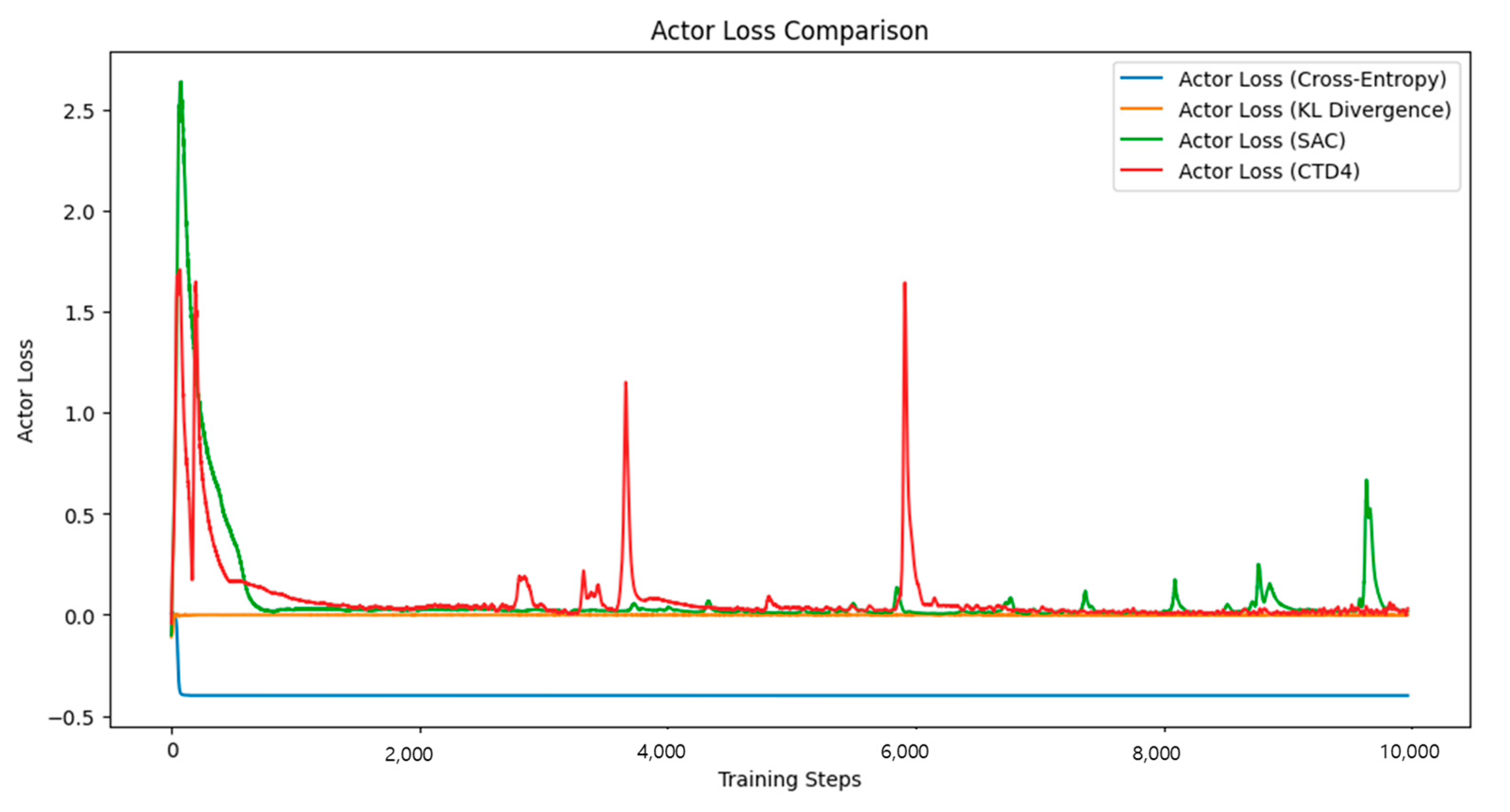
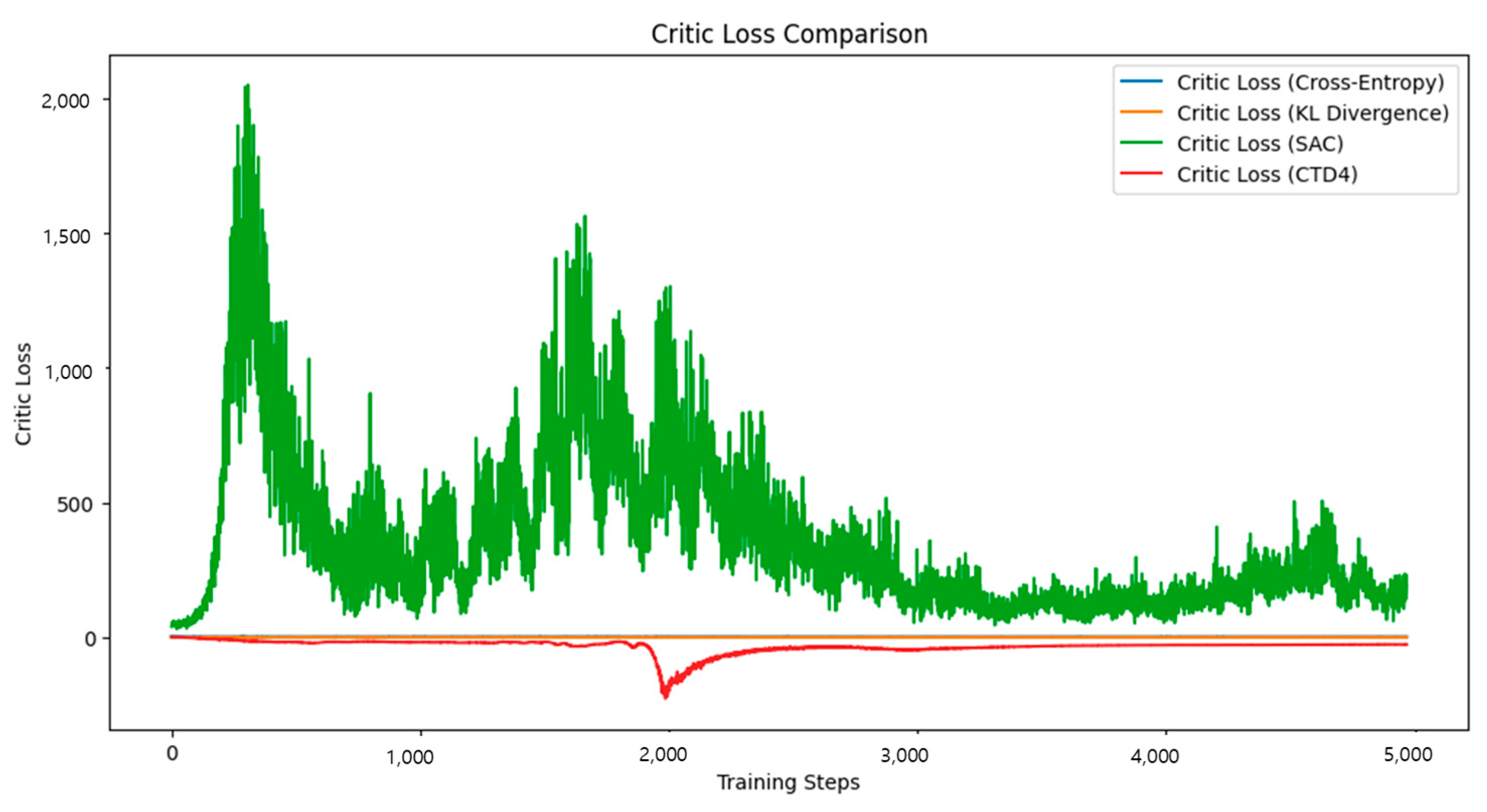
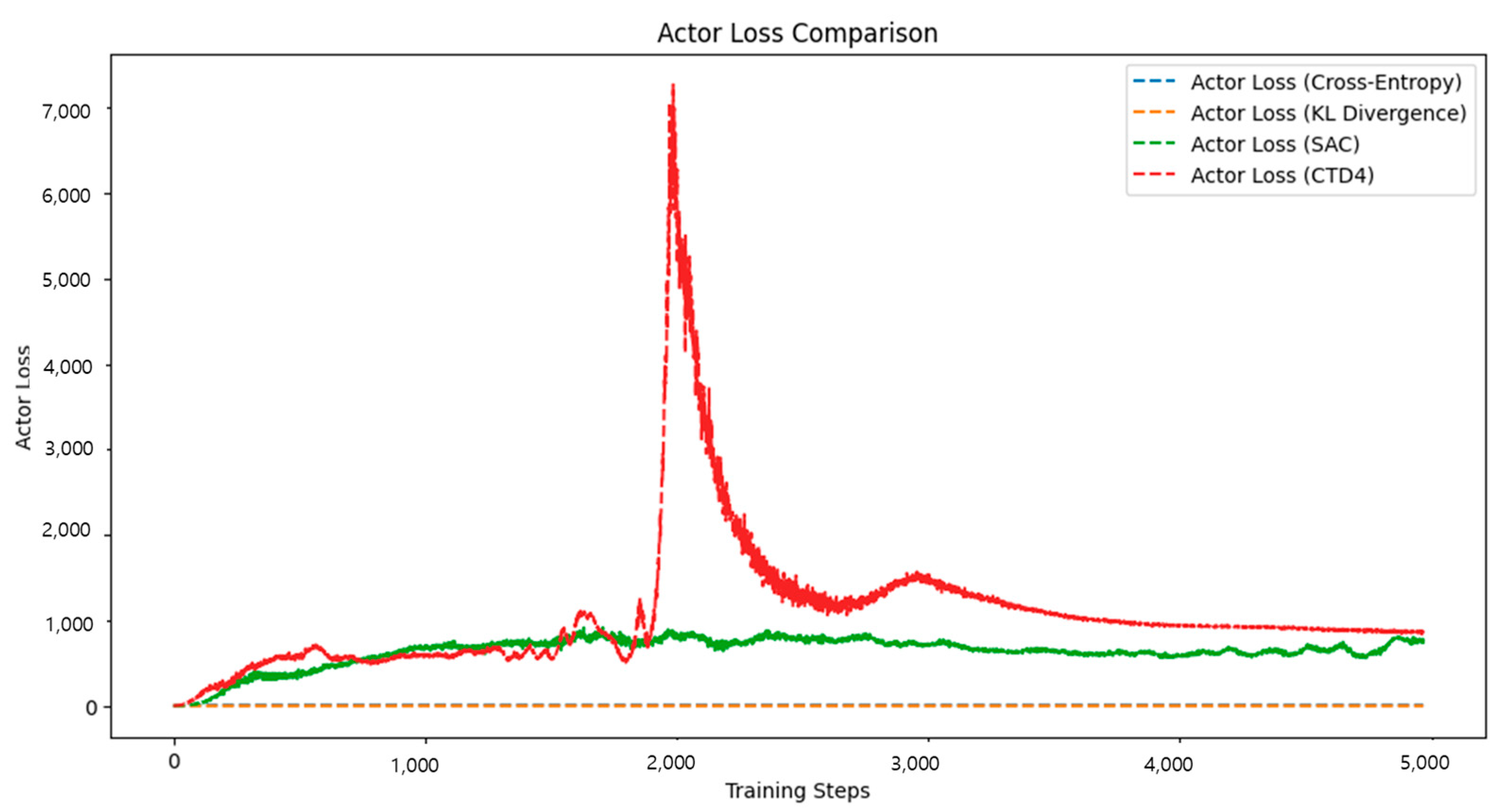
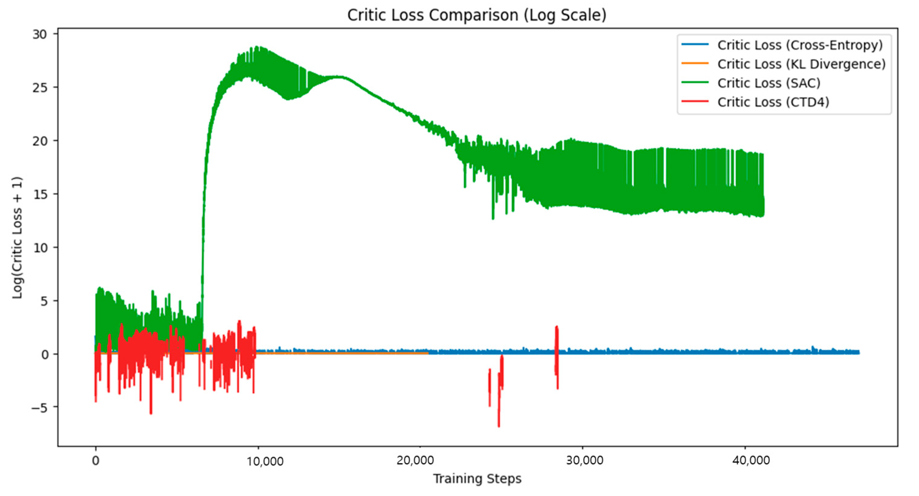
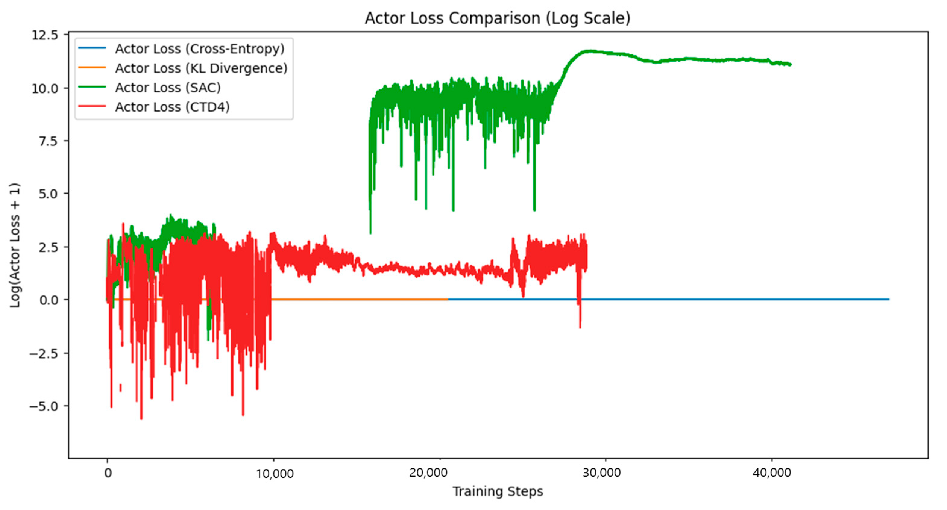
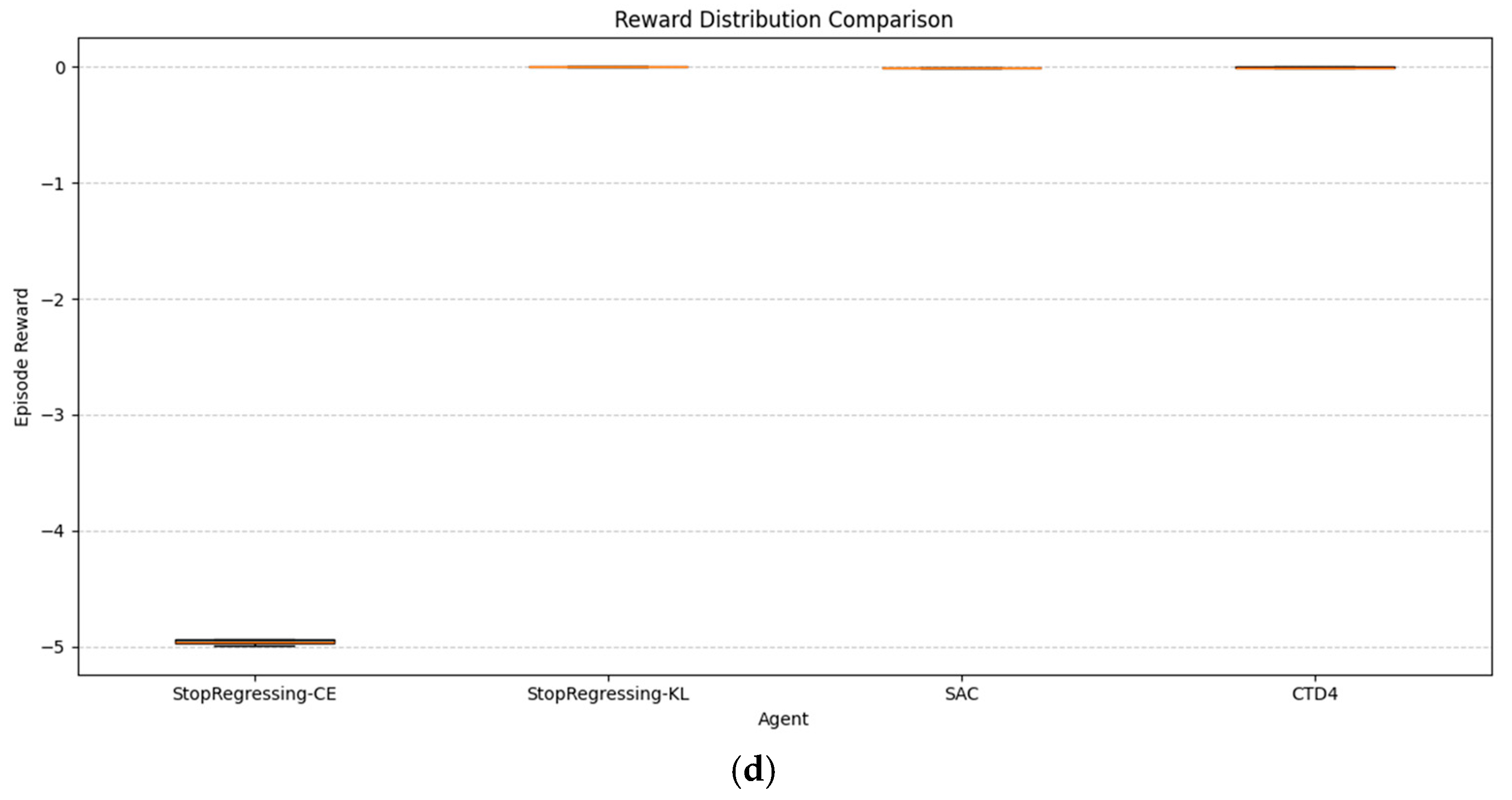
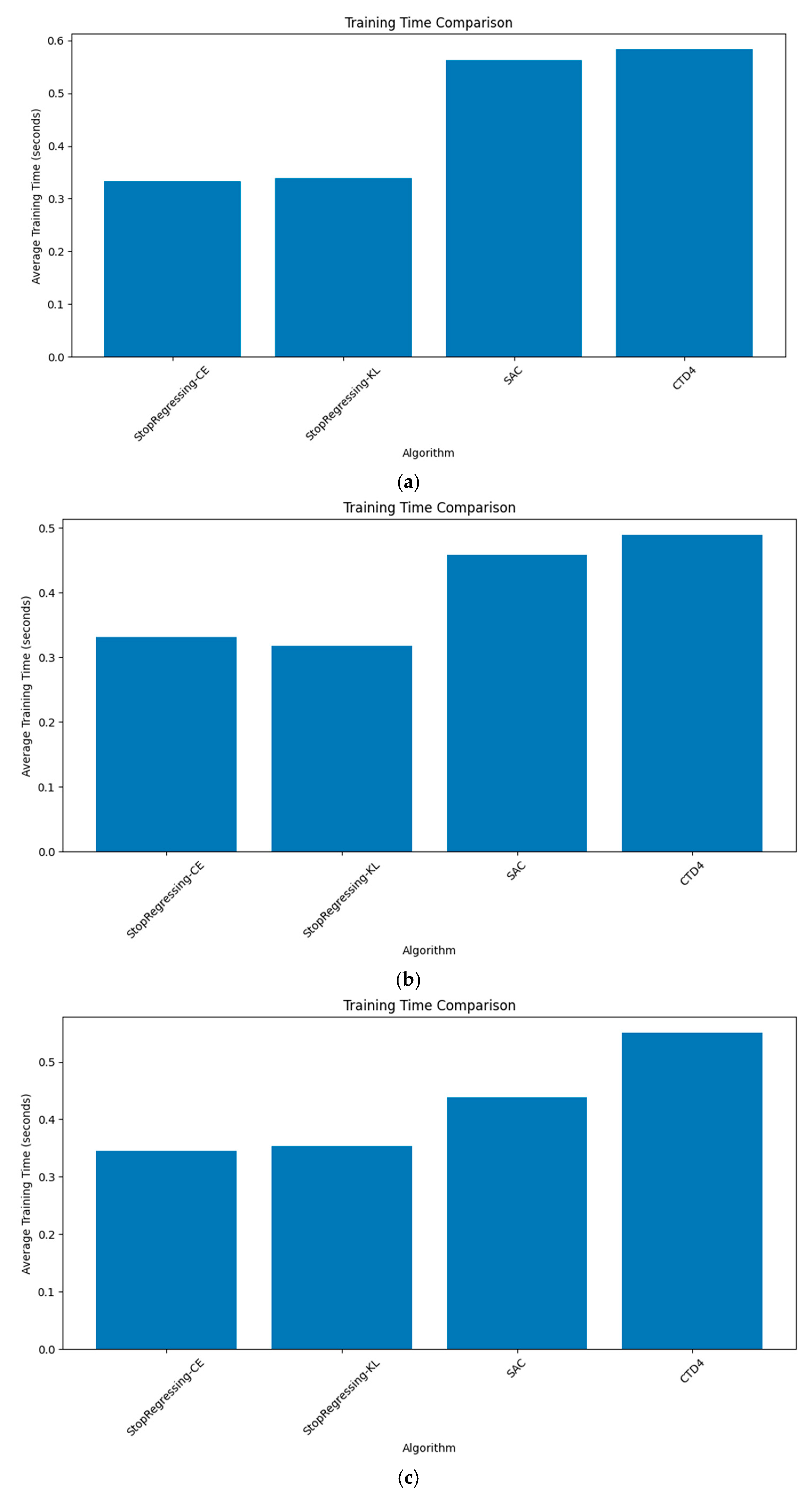
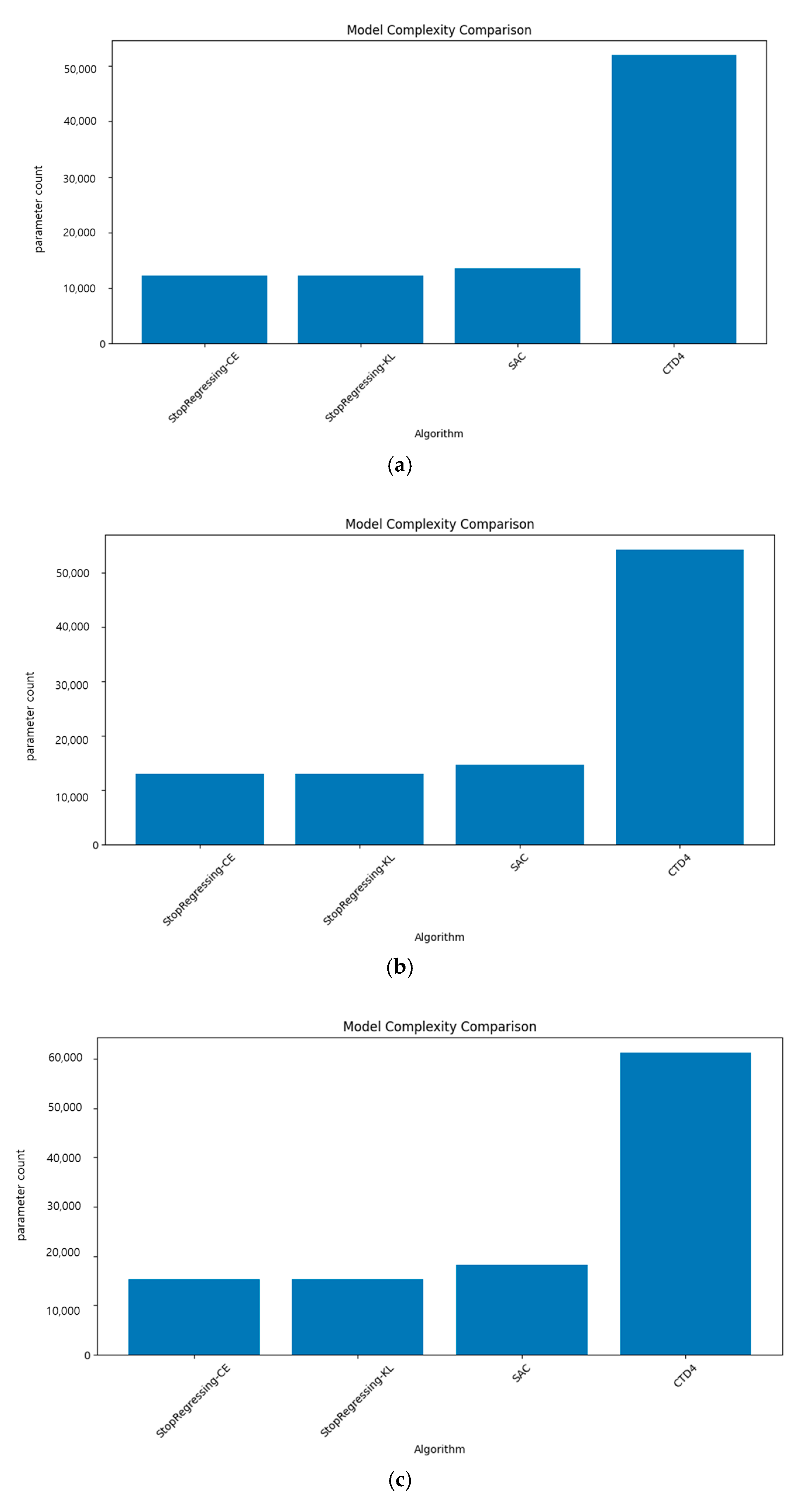
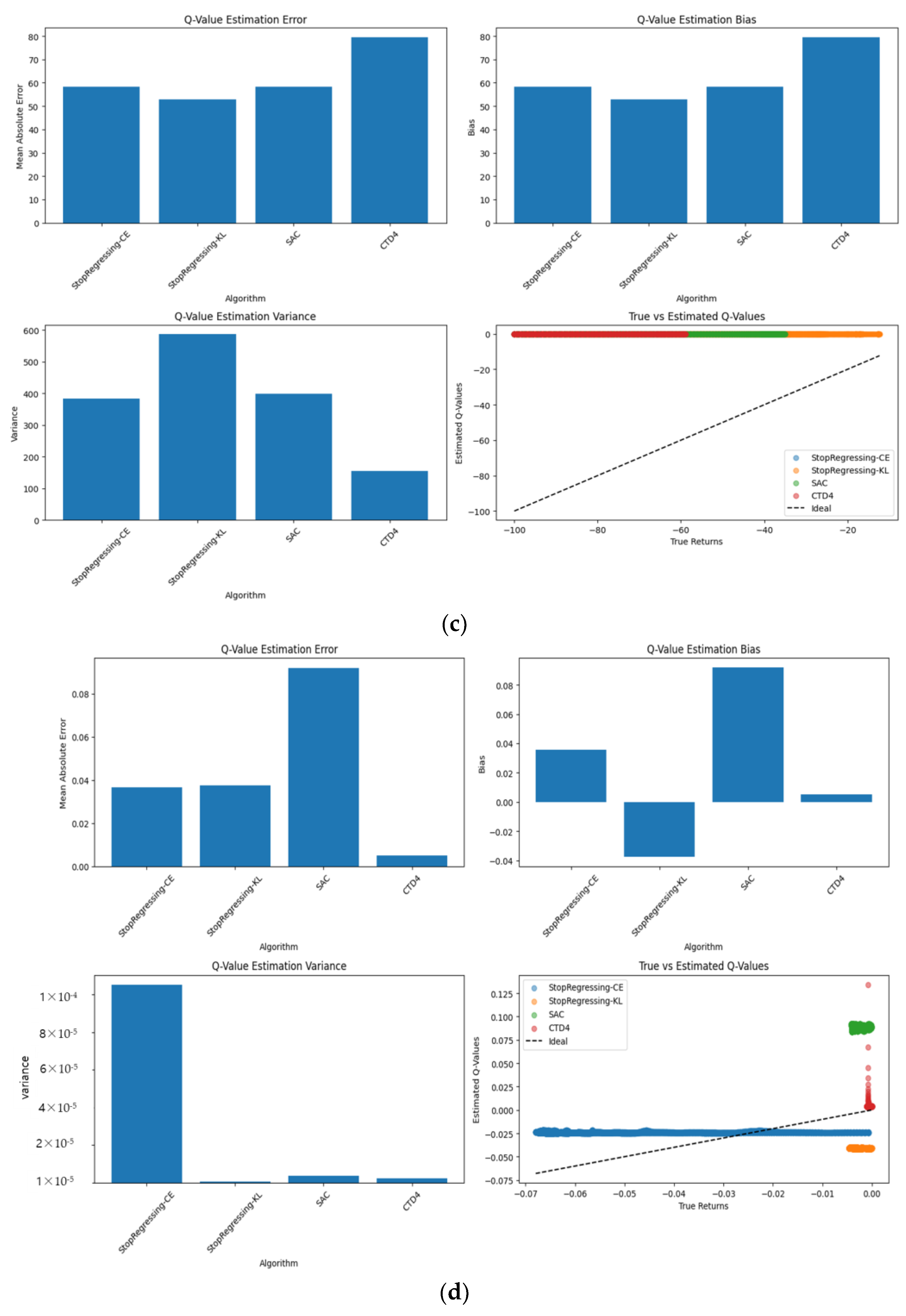
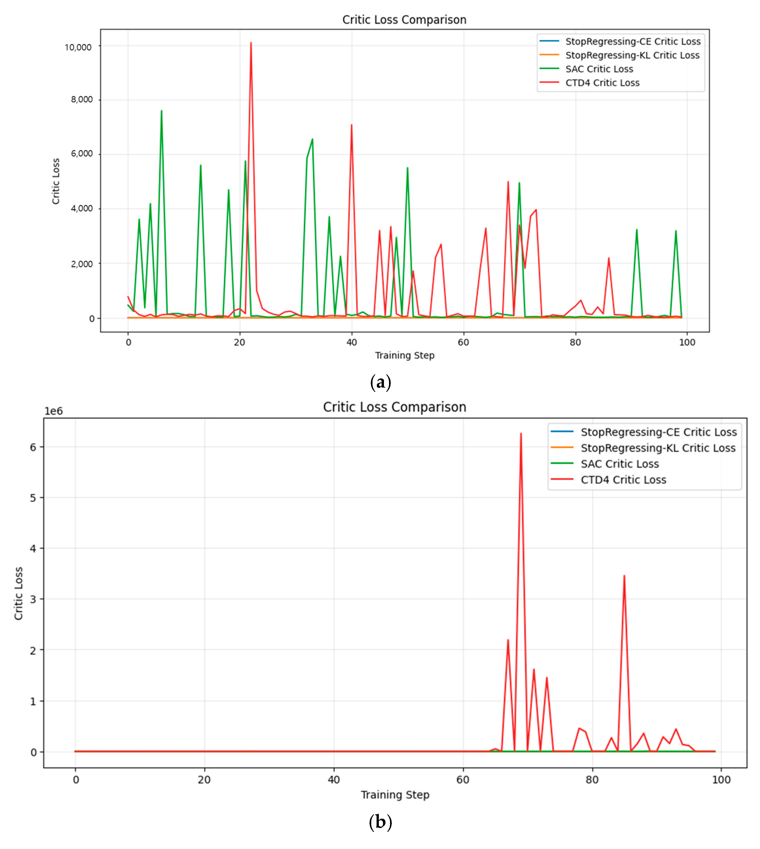
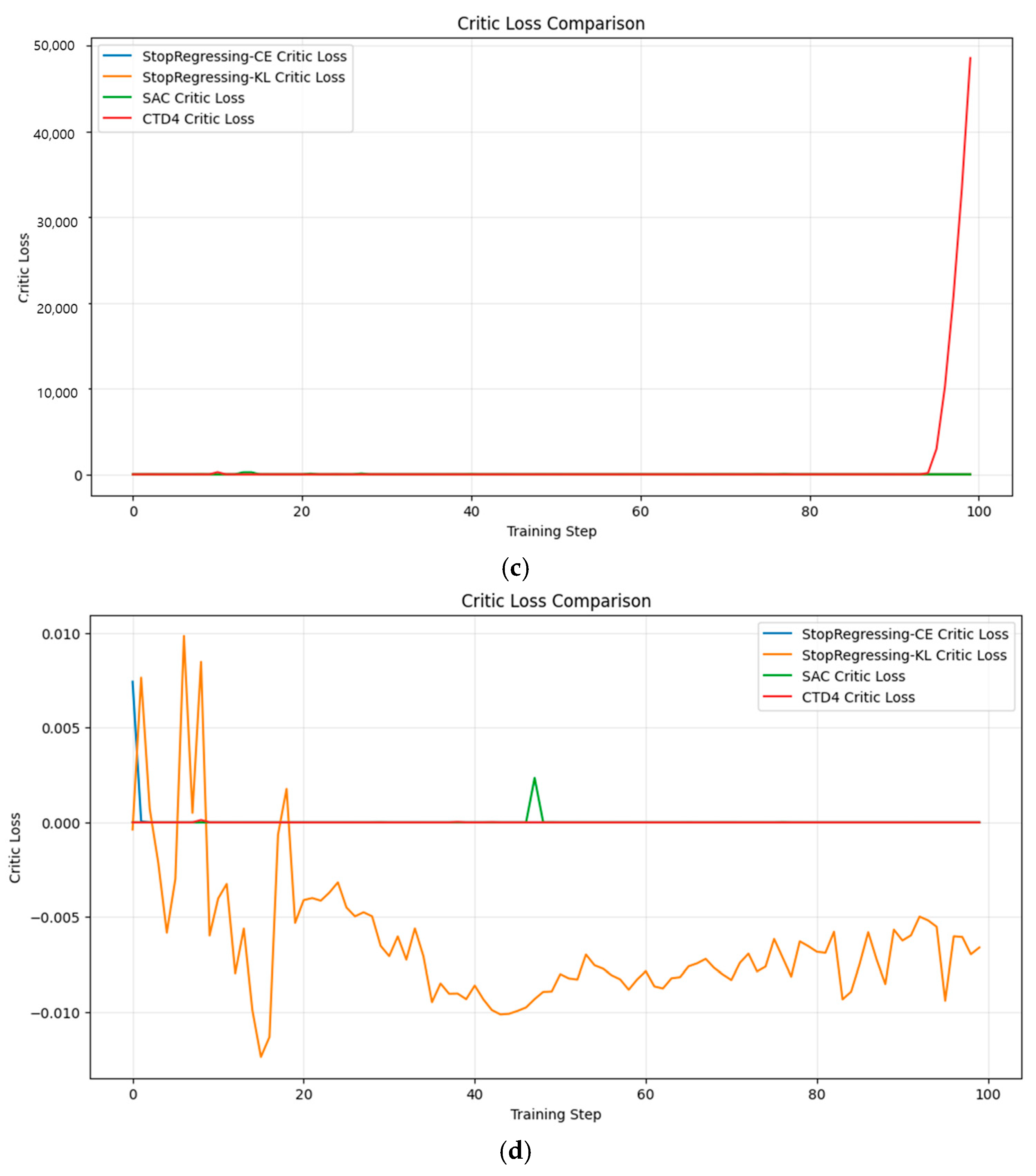
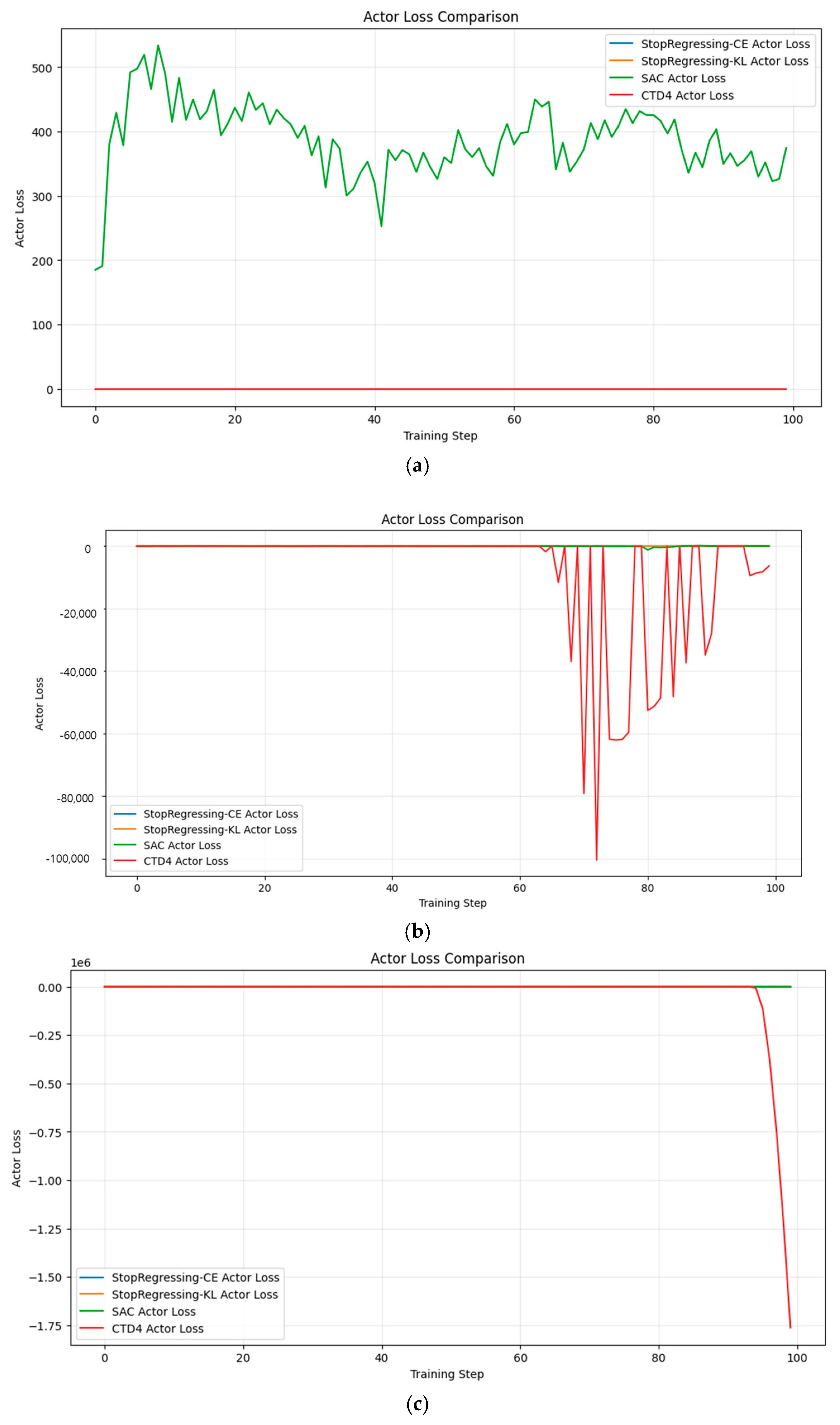