Performance Evaluation of ARIMA, Autoformer, and Symmetric LSTNFCL Models for Traffic Accident Emergency Prediction

Abstract

The prediction of pre-hospital medical emergencies based on historical timing data holds significant potential for enhancing individual safety. In this study, we constructed ARIMA (Autoregressive Integrated Moving Average Model), Autoformer, and the structurally symmetric deep learning model LSTNFCL (Long-Short-Term Network with Conv2Former, CBAM (Convolutional Block Attention Module), and LSTM) using the time-period symmetric pre-hospital traffic accident medical emergency calls in Chengdu from 1 January 2022 to 31 December 2023. We systematically evaluated the prediction efficiency of the three models on pre-hospital traffic accident medical emergency call demand. The experiments show the following: The MAE (mean absolute error) of Autoformer is 0.849 and the RMSE (root mean square error) is 0.922, but its inference takes longer; LSTNFCL achieves competitive performance with an MAE of 1.681 and an RMSE of 3.301 under a lightweight architecture by integrating LSTM (Long Short-Term Memory), Conv2Former, and CBAM modules. It demonstrates notably superior computational efficiency and reasoning time compared to ARIMA. Furthermore, it surpasses Autoformer in terms of efficiency and reasoning time. Ablation experiments demonstrate that the Conv2Former module reduces the MSE (mean squared error) by 21%, while the CBAM module further optimizes the MAPE (mean absolute percentage error) to 0.891%. This study provides a prediction scheme that balances accuracy and real-time performance for pre-hospital emergency systems, and the results show that Autoformer is suitable for offline high-precision scenarios, while LSTNFCL is more suitable for real-time prediction needs with resource constraints. Focusing on the public safety, this paper offers an effective early prediction method for the pre-hospital emergency medical system.

1. Introduction

The World Health Organization (WHO) reported in 2023 that globally about 1.3 million people die each year from road traffic accidents (2.3% of all deaths), resulting in a loss of 3–5% of global GDP (about USD 1.8 trillion/year) [1]. This underscores the vital necessity to reinforce the capabilities of pre-hospital medical emergency services and to improve the capacity of monitoring and early prediction of the emergency system. A significant proportion of pre-hospital medical emergency calls are from traffic accidents, which highlights the necessity for the development of a predictive model. However, researchers have conducted little research in this field.

The data pertaining to pre-hospital traffic accident emergency calls exhibits patterns and trends over time. The collated data comprise a series of data points arranged in chronological order, which reflects the state of a system or process at different points in time. Consequently, this paper treats the aforementioned data as time series data for the purposes of analyzing and predicting the number of future callers. Time series analysis methods leverage the relationship between the current and past values of the series, as well as stochastic factors, to construct prediction models with a certain degree of accuracy [2]. These include autoregressive (AR), moving average (MA), autoregressive moving (ARMA), and autoregressive integrated moving average (ARIMA) models. Among these models, the ARIMA model [3] excels at extracting deterministic information from non-stationary time series, and achieves this efficiently by using the characteristics of the difference method. This has important applications in the study and forecasting of fluctuating time series. Thirugiri et al. [4] developed an ARIMA-based mobility prediction model to predict the future mobility speed of nodes in a mobile autonomous network (MANET). Dey et al. [5] developed and compared a variety of linear and nonlinear regression models, as well as the ARIMA model, with the objective of predicting gasoline demand in India. Zhao et al. [6] used an ARIMA model to predict the number of COVID-19 confirmed cases using a dataset from 1 November 2021 to 17 February 2022. However, the ARIMA model can only capture linear relationships in a time series and fails to model complex nonlinear patterns, making it difficult to capture dependencies between distant time steps.

The inherently temporal nature of time series data is a key property that deep learning models can capture, which is particularly significant when handling sequence data. For example, the Hetero-ConvLSTM model, which uses heterogeneous spatiotemporal data, and the traffic accident prediction method, which employs the LSTM-GBRT model, are adept at handling complex data [7,8], but the model fusion architecture is complex, requires multimodal data alignment, and incurs high data preprocessing costs in real-world applications. These models not only enhance the precision of prediction, but also offer novel insights into traffic management. Furthermore, deep-learning-based frameworks for traffic accident severity prediction have demonstrated their potential in accident consequence assessment [9], but are not dynamically adaptable enough to real-time data to handle sudden road condition changes. A deep learning approach was employed to construct models for time series research utilizing Convolutional Neural Networks (CNNs), Recurrent Neural Networks (RNNs) [10], Long Short-Term Memory (LSTM) [11], Gated Recurrent Unit (GRU) [12], and Transformer [13]. Lai et al. [14] synthesized the proposed LSTNet (Long and Short-term Time series Network) model by combining the network structure of CNN with RNN, LSTM, and GRU, thereby achieving superior results in the exchange-rate dataset, but lacked the self-attention module to integrate the entire time series to improve the overall feature relevance of the model to the data. Wu et al. [15] employed the Transformer to construct the Autoformer model and conducted model validation on six datasets (ETT, Electricity, Exchange, Traffic, Weather, and ILI) spanning diverse domains. The best results were achieved on all datasets, but the model parametric quantities and inference times were large, and the computational resource requirements were too high to be deployed on lightweight devices. However, the Transformer model, due to its attention mechanism, exhibits an increase in inference time with an increase in the number of parameters in a time series. Li et al. [16] proposed a novel adaptive traffic signal control method based on periodic signal timing and traffic flow prediction, which combines a mixture of Kalman filtering and LSTM to achieve traffic flow prediction. Cai et al. [17] proposed the MHA-Net multiscale higher-order attention mechanism network, which demonstrated a more lightweight performance than the Transformer model, but with lower accuracy in model prediction. This was achieved by reducing the model parameters and inference time. However, there is a paucity of research in the traffic accident emergency prediction field.

Regarding traffic flow prediction, Che et al. [18] proposed a novel traffic flow prediction method based on the fusion of static and dynamic maps, and verified the performance of the proposed method. Wang et al. [19] proposed a hybrid framework combining Long Short-Term Memory Neural Networks (LSTM NNs) and Bayesian Neural Networks (BNNs) for real-time traffic flow prediction and uncertainty quantification based on sequential data. Dong [20] proposed a new integrated entropy cloud model, which includes two algorithms: fused cloud model inference based on DS evidence theory and cloud model inference and prediction based on compensatory mechanism, which are designed to solve the problem of short-term traffic flow prediction by utilizing a cloud model of the historical traffic data to guide the short-term prediction in the future. Wang et al. [21] introduced an innovative traffic flow prediction method, ASTRformer, which emphasizes the integration of spatial and temporal information from historical data through an adaptive spatiotemporal relationship learning mechanism that integrates feature embedding with adaptive spatial and temporal embedding. Chen et al. [22] proposed a traffic flow prediction model based on sequence to sequence time graph convolutional network, designing an innovative Seq2seq architecture based on time graph convolutional network to capture the spatiotemporal features of traffic flow. However, the above study lacks a comparison with traditional time series prediction models (e.g., ARIMA, Autoformer). To address this gap, we conduct statistical characterization and autocorrelation analysis of the measured data, aiming to identify temporal change patterns and forecast future values based on historical observations. In this study, we use the pre-hospital traffic accident emergency calls data of Chengdu City to train three models. The models considered are ARIMA, LSTNFCL (Long-Short-Term Network with Conv2Former, CBAM (Convolutional Block Attention Module), and LSTM) and Autoformer. The optimal model is selected based on the criteria of mean absolute error (MAE) and root mean square error (RMSE). The initial step is to select a historical time series data set of a specified length, which will serve as the modeling dataset. Subsequently, the modeling dataset is evaluated in terms of its smoothness and stochasticity, and an appropriate model is selected for modeling purposes. The main contribution of the model is to improve the LSTNet model and propose a novel LSTNFCL timing prediction framework. First, in the feature extraction stage, the Conv2Former module is introduced to combine the convolutional operation with the self-attention mechanism, which enhances the model’s ability to jointly model local features and global timing dependencies; meanwhile, the CBAM attention mechanism is integrated in the feature fusion session to dynamically adjust the key feature weights through the channel-space dual visual attention. Secondly, at the temporal modeling level, a hybrid loop cell architecture of GRU, LSTM, and RNN is constructed to comprehensively capture the multiscale patterns of temporal data by taking advantage of the complementary nature of different gating mechanisms. In addition, by optimizing the feature interaction paths and adjusting the residual connection structure, the efficient fusion of multilevel features is achieved, which further strengthens the nonlinear representation ability of the model. Then, the loss function MSE is optimized using stochastic gradient descent, which in turn optimizes the model parameters and results in an optimized model. Finally, the model is utilized to predict future pre-hospital traffic accident emergency calls.

1.1. Symmetry in Traffic Patterns

Pre-hospital traffic accident emergency calls in Chengdu exhibit both temporal symmetry and asymmetry. Cyclic symmetry is manifested by mirrored demand patterns during daily peak hours (e.g., 8:00–9:00 vs. 17:00–18:00) and weekly cycles, with weekday peaks forming a self-similar temporal structure. Conversely, holiday diversions and irregular events lead to asymmetry. The LSTNFCL model proposed in this paper decomposes the temporal signal into symmetric and asymmetric components via Conv2Former-CBAM. The GRU layer maintains daily symmetry via reset gates, the LSTM forgetting gates isolate holiday-induced asymmetries, and parallel RNN branching strengthens the stability of short-term patterns. Adaptive residual concatenation dynamically reweights the symmetric/asymmetric features of each layer, and LSTNFCL suppresses overfitting to historical symmetries by suppressing overfitting when dealing with holiday data. Autoformer captures temporal symmetry through its global self-attention mechanism and positional encoding, and recognizes periodic patterns by calculating pairwise correlations across all timestamps. However, its static attention matrix tends to overfit historical symmetries while lacking an explicit mechanism to isolate asymmetric events. In contrast, the LSTNFCL proposed in this study explicitly splits the symmetric/asymmetric components through a hybrid operation of Conv2Former and adaptively reweights them using CBAM to achieve multiscale temporal filtering, which has been validated on data with Chengdu traffic.

1.2. Organization of the Paper

The remainder of this paper is organized as follows. Section 2 describes the methodology for analyzing and predicting pre-hospital traffic accident medical emergency calls in Chengdu, including data processing and modeling. Section 3 validates model performance on historical data, highlighting the lightweight LSTNFCL model’s competitive accuracy with computational efficiency. Section 4 provides an in-depth analysis of the differences between the different models and their applicability scenarios. The last section summarizes the research results of the whole paper, reiterates the importance and practical application value of the research, and proposes possible future research directions.

2. Methods

2.1. Data Preparation

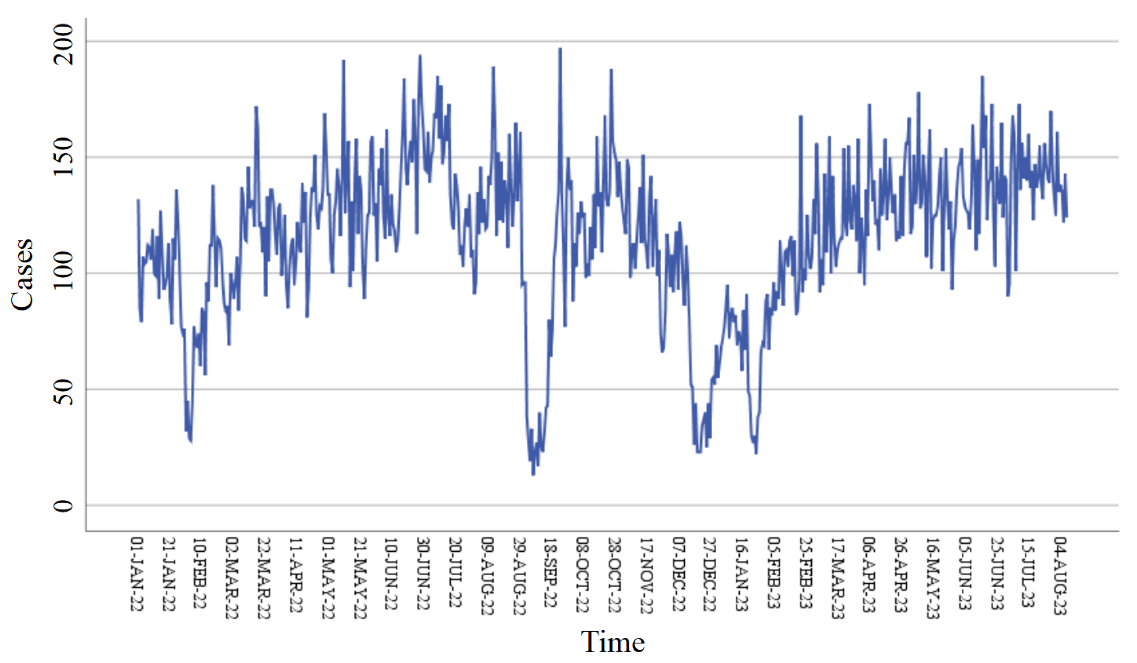
We used pre-hospital medical emergency calls in Chengdu from 1 January 2022 to 31 December 2023, provided by the Chengdu Medical Emergency Center. All data are updated daily. In this study, 730 observations were divided into a training set and a validation set, of which 80% was the training set and the rest (20%) was the test set. The dataset from 1 January 2022 to 6 August 2023 was considered as the training set, and the data from 7 August 2023 to 31 December 2023 was considered as the validation set.

For non-stationary time series, normalization preserves statistical symmetry through linear transformation, while second-order differencing converts asymmetric trends into symmetric and stationary sequences by eliminating trend components. This symmetry transformation is a critical prerequisite for ARIMA modeling.

2.2. ARIMA Model

The ARIMA model is a commonly used non-smooth time series forecasting model, which consists of an autoregressive (AR) model and a sliding average (MA) model. The ARIMA model is generally denoted as ARIMA(p,d,q) (p,d,q are the orders of the AR model, the signal difference and the MA model, respectively), which is an extension of ARMA(p,q). The ARIMA model can only be used for smooth time series, while for the non-smooth time series $Y_t$, ARIMA transforms $Y_t$ into a smooth time series $X_t$ by d-order signal differencing, and then fits the smooth time series $X_t$ with the ARMA(p,q) model, which is the ARMA(p,q) model:

$$\begin{array}{c}\hfill X_t=\sum _{i=1}^p{\varphi }_i{X}_{t-i}+\sum _{j=1}^q{\theta }_j{\epsilon }_{t-j}+{\epsilon }_t\end{array}$$

(1)

where ${\varphi }_i$ and ${\theta }_j$ are autoregressive coefficients and sliding average coefficients, respectively; ${\epsilon }_t$ is a white noise sequence obeying a normal distribution with mean 0. The modeling process of ARIMA is as follows:

• The ADF and KPSS unit root methods are used to test the smoothness of the time series data, respectively.
• If the smoothness test is not passed, the time series is converted to a smooth time series by performing a d-order difference.
• The models are ranked using the Bayesian information criterion (BIC).
• The time series are fitted using a fixed-order model, and the model parameters are estimated using great likelihood estimation.
• The autocorrelation of the residuals of the model fit is tested. The closer the residuals are to the white noise distribution, the more fully the useful information in the time series is extracted.
• After passing the residual test, the specified ARIMA model can be used for time series forecasting. If the residual test is not passed, the model will be re-ordered.

For the ARIMA model, its symmetry arises from the stationarity requirement enforced through differencing, which assumes invariance in statistical properties under time translation. This symmetry enables ARIMA to model linear temporal patterns but restricts its ability to adapt to non-stationary dynamics. In contrast, the LSTNFCL architecture inherently breaks such symmetry via its gating mechanisms, allowing adaptive learning of time-varying patterns in non-stationary regimes.

2.3. LSTNFCL Model

Recurrent Neural Networks (RNNs) [23] are a class of neural network structures specialized in processing sequence data, and are characterized by the possibility of introducing recurrent connections to process the temporal information of sequence data. The specific inference process is as follows, and its structure is shown in Figure 1.

$$\begin{array}{cc}\hfill & a^{<t>}=g(W_{aa}{a}^{<t-1>}+W_{ax}{x}^{<t>}+b_a)\hfill \\ \hfill & {\overline{y}}^{<t>}=g(W_y{a}^{<t>}+b_y)\hfill \end{array}$$

(2)

In the above calculation, y is the information output, a is the information input, W is the weight information, and g is the activation function. It is possible to make the information after a certain time propagation also retain the information of the previous period of time, to have the effect of a short time attention mechanism.

However, the traditional RNN structure suffers from the problems of gradient vanishing and gradient explosion, which leads to difficulties in processing long sequence data and capturing long-term dependencies. In order to solve this problem, the Long Short-Term Memory Network (LSTM) [24] is proposed. The LSTM introduces three key gating structures: input gate, forgetting gate, and output gate, through which the flow of information can be better controlled and long-term dependencies can be captured efficiently, which mitigates the problem of gradient vanishing and gradient exploding and enables LSTM to perform better in dealing with sequential tasks that require long-term memory.

Similar to LSTM, the gated recurrent unit GRU is another structure proposed to solve the gradient problem of the RNN. The GRU [25] is more simplified compared to LSTM, containing only two gating structures, the update gate and the reset gate, which reduces the number of parameters, while maintaining a better performance performance to a certain extent. Therefore, in some scenarios with high requirements on model size and computational efficiency, the GRU model is usually used to solve the gradient problem of RNN. The specific reasoning of LSTM and the GRU is as follows, and its model structure diagram is shown in Figure 2 and Equation (3).

$$\begin{array}{cc}\hfill & \left(\begin{array}{c}i\\ f\\ O\\ g\end{array}\right)=\left(\begin{array}{c}\sigma \\ \sigma \\ \sigma \\ tanh\end{array}\right)W\left(\begin{array}{c}{h}_{t-1}\\ x_t\end{array}\right)\hfill \\ \hfill & c_t=f·c_{t-1}+i·g\hfill \\ \hfill & h_t=O·tanh\left(c_t\right)\hfill \end{array}$$

(3)

where f and i are forgetting gate and input gate functions, respectively; h is the past information output; $c_{t-1}$ synthesizes the past input information; O is the final output; $\sigma$, tanh, and u are the activation functions; and W is the weight information. The GRU, which is similar to this one, includes only the update gate ${\mathrm{\Gamma }}_u$ and the reset gate ${\mathrm{\Gamma }}_r$:

$$\begin{array}{cc}\hfill & {\stackrel{⌢}{c}}_t=u(W_c[{\mathrm{\Gamma }}_r\ast c_{t-1},x_t]+b_c)\hfill \\ \hfill & c_t={\mathrm{\Gamma }}_u{\stackrel{⌢}{c}}_t+(1-{\mathrm{\Gamma }}_u)c_{t-1}\hfill \\ \hfill & h_t=u(W_h{a}_t+b_y)\hfill \\ \hfill & {\mathrm{\Gamma }}_u=\sigma (W_u[c_{t-1},x_t]+b_u)\hfill \\ \hfill & {\mathrm{\Gamma }}_r=\sigma (W_r[c_{t-1},x_t]+b_r)\hfill \end{array}$$

(4)

where W, b are the weights and biases of each parameter, respectively. The importance of c, x is learned, and weight information is obtained by ${\mathrm{\Gamma }}_u$ and ${\mathrm{\Gamma }}_r$, respectively.

As illustrated in Figure 3, the LSTNet method [26] integrates multiple deep learning network structures. It employs a one-dimensional convolutional network to extract data features, followed by an RNN network for temporal feature extraction. Additionally, a GRU structure is embedded within the RNN-skip architecture to capture long-term time series patterns and periodic dependencies. Global attention is implemented via an attention mechanism, while the autoregressive (AR) process is simulated using a linear multilayer perceptron (MLP) through a HighWay module, ensuring the desired output dimensionality.

This paper introduces the LST-Skip model, which combines the LSTM framework with other deep learning architectures and an attention mechanism. This model adopts a structurally symmetric design, enhancing computational efficiency in time series prediction. The symmetry balances the model’s computational load, reduces parameter counts and inference times, and improves generalization capabilities. By capturing bidirectional dependencies in time series data, it ensures balanced forward and backward information flows, mitigating the risk of local optima. Furthermore, the model emphasizes key time points, improving prediction accuracy and leveraging LST-Skip to incorporate prior knowledge of periodicity into the sequence.

Experimental results demonstrate that this model performs exceptionally well in time series forecasting. To address the asymmetry inherent in the original LSTNet model, we propose the LSTNFCL model—a structurally symmetric architecture that offers superior performance and stability compared to LSTNet. The structure of the LSTNFCL model is depicted in Figure 4.

By optimizing the LSTNet model, we propose the LSTNFCL model, which is a complex neural network architecture designed for time series analysis and forecasting. The model integrates a convolutional layer for feature extraction, an attentional mechanism to enhance feature representation, and a recursive layer to capture temporal dependencies. By combining these components, the LSTNFCL model is able to efficiently integrate information from different branches and, thus, excel in tasks that require spatiotemporal understanding of data. In addition, the model introduces an autoregressive layer to further capture the dynamics in the time series, and finally achieves accurate prediction results through the linear and additive layers.

The LSTNFCL model proposed in this paper decomposes the temporal signal into symmetric and asymmetric components via Conv2Former-CBAM. The GRU layer maintains daily symmetry via reset gates, the LSTM forgetting gates isolate holiday-induced asymmetries, and parallel RNN branching strengthens the stability of short-term patterns. Adaptive residual concatenation dynamically reweights the symmetric/asymmetric features of each layer, and LSTNFCL suppresses overfitting to historical symmetries by suppressing overfitting when dealing with holiday data.

2.4. Autoformer Model

Since Transformer was proposed in 2017, starting as a solution to problems in natural language, the self-attention mechanism makes it possible to consider all positions in the input sequence at the same time. Therefore, it better captures global dependencies and is suitable for modeling entire time series. In addition, the Transformer model can be computed in parallel, thus allowing faster training and inference when dealing with time series of longer lengths. However, for longer time series, the computational cost of the Transformer model becomes very high due to the fact that the autoattention mechanism needs to take into account the information of all the positions, which can lead to an increase in computational complexity with the increase in the length of the sequence.

As shown in Figure 5, the Autoformer, proposed by Zeng et al. [27], breaks through the traditional method of sequence decomposition as preprocessing and proposes the decomposition architecture, which is able to decompose more predictable components from complex time patterns.

Based on the theory of stochastic process, the autocorrelation mechanism is proposed to replace the attention mechanism of point-wise connection, to realize series-wise connection and O(nlogn) complexity, and to break the bottleneck of information utilization. The model uses encoder and decoder patterns. The encoder part gradually eliminates the trend term to obtain the time series detection and mainly calculates the period term S, where X is a hidden variable. (Remember SeriesDecomp is $SD$, AutoCorrelation is $AC$, and FeedForward is $FF$):

$$\begin{array}{cc}\hfill & S_{en}^{l,1}=SD(AC\left(X_{en}^{l-1}\right)+X_{en}^{l-1})\hfill \\ \hfill & S_{en}^{l,2}=SD(FF\left(S_{en}^{l,1}\right)+S_{en}^{l,1})\hfill \end{array}$$

(5)

The decoder periodic term is

$$\begin{array}{cc}\hfill & S_{de}^{l,1},T_{de}^{l,1}=SD(AC\left(X_{de}^{l-1}\right)+X_{de}^{l-1})\hfill \\ \hfill & S_{de}^{l,2},T_{de}^{l,2}=SD(AC(S_{de}^{l,1},X_{en}^N)+S_{de}^{l,1})\hfill \\ \hfill & S_{de}^{l,3},T_{de}^{l,3}=SD(FF\left(S_{de}^{l,2}\right)+S_{de}^{l,2})\hfill \\ \hfill & T_{de}^l=T_{de}^{l-1}+\sum _{i=1}^3{W}_{l,i}\ast T_{de}^{l,i}\hfill \end{array}$$

(6)

Autoformer captures temporal symmetry through its global self-attention mechanism and positional encoding, and recognizes periodic patterns by calculating pairwise correlations across all timestamps. However, its static attention matrix tends to overfit historical symmetries while lacking an explicit mechanism to isolate asymmetric events.

2.5. Evaluation of the Prediction Performance

In this article, we use mean absolute error (MAE) and root mean square error (RMSE) to assess the predictive performance of the model; the smaller the value of MAE and RMSE, the better the predictive ability of the model. These equations and other metrics, including BIC (Bayesian information criterion), RSE (relative squared error), RAE (relative absolute error), CORR (correlation coefficient), MAPE (mean absolute percentage error), MSE (mean squared error), and MSPE (mean squared percentage error), are shown below.

$$\begin{array}{cc}\hfill \mathrm{BIC}& =kln\left(n\right)-2ln\left(\widehat{L}\right)\hfill \end{array}$$

(7)

$$\begin{array}{cc}\hfill \mathrm{RSE}& ={\displaystyle \frac{{\sum }_{i=1}^n{(y_i-{\widehat{y}}_i)}^2}{{\sum }_{i=1}^n{(y_i-\overline{y})}^2}}\hfill \end{array}$$

(8)

$$\begin{array}{cc}\hfill \mathrm{RAE}& ={\displaystyle \frac{{\sum }_{i=1}^n|y_i-{\widehat{y}}_i|}{{\sum }_{i=1}^n|y_i-\overline{y}|}}\hfill \end{array}$$

(9)

$$\begin{array}{cc}\hfill \mathrm{CORR}& ={\displaystyle \frac{{\sum }_{i=1}^n(y_i-\overline{y})({\widehat{y}}_i-\overline{\widehat{y}})}{\sqrt{{\sum }_{i=1}^n{(y_i-\overline{y})}^2·{\sum }_{i=1}^n{({\widehat{y}}_i-\overline{\widehat{y}})}^2}}}\hfill \end{array}$$

(10)

$$\begin{array}{cc}\hfill \mathrm{MAPE}& ={\displaystyle \frac{100\%}{n}}\sum _{i=1}^n\left|{\displaystyle \frac{y_i-{\widehat{y}}_i}{y_i}}\right|\hfill \end{array}$$

(11)

$$\begin{array}{cc}\hfill \mathrm{MSE}& ={\displaystyle \frac{1}{n}}\sum _{i=1}^n{(y_i-{\widehat{y}}_i)}^2\hfill \end{array}$$

(12)

$$\begin{array}{cc}\hfill \mathrm{MSPE}& ={\displaystyle \frac{1}{n}}\sum _{i=1}^n{\left({\displaystyle \frac{y_i-{\widehat{y}}_i}{y_i}}\right)}^2\hfill \end{array}$$

(13)

$$\begin{array}{cc}\hfill \mathrm{MAE}& ={\displaystyle \frac{{\sum }_{i=1}^n\left|y_i-{\widehat{y}}_i\right|}{n}}\hfill \end{array}$$

(14)

$$\begin{array}{cc}\hfill \mathrm{RMSE}& =\sqrt{{\displaystyle \frac{{\sum }_{i=1}^n{\left(y_i-{\widehat{y}}_i\right)}^2}{n}}}\hfill \end{array}$$

(15)

where $\widehat{y_i}$ denotes the predicted value for the i-th observation, $y_i$ denotes the (true) value for the i-th observation, n denotes the number of samples, $\overline{y}$ denotes the average of the observations, $\overline{\widehat{y}}$ denotes the average of the predicted values, k denotes the number of model parameters, and $\widehat{L}$ denotes the value of the likelihood function.

3. Results

This study adopts a systematic data preprocessing process to ensure the reproducibility of the experiment. Raw data were first processed for missing values: data segments with consecutive missing time steps less than 3 were filled in by linear interpolation, and long-term missing segments were directly excluded; outliers were identified by the 3$\sigma$ principle and corrected based on sliding-window mean smoothing. All features were divided into training and testing sets after min–max normalization (8:2). The histogram of the distribution after data preprocessing is shown in Figure 6.

3.1. ARIMA Model Results

The pre-hospital emergency call data in Chengdu exhibit significant fluctuations, with periodic upward and downward trends over time (Figure 7). To address this, we applied second-order differencing to stabilize the series. The resulting differenced data display stochastic yet stable behavior, confirming their stationarity (Figure 8), which is further supported by the ADF test results ($t=-18.394$, p < 0.01).

To determine the ARIMA model parameters $(p,q)$, we analyzed the ACF and PACF plots (Figure 9 and Figure 10). The differenced series shows a truncated tail at lags 1 or 2 and an exponentially decaying tail spanning lags 1 to 4. Based on these patterns, we evaluated multiple candidate models: ARIMA(1,2,1), ARIMA(1,2,2), ARIMA(1,2,3), ARIMA(1,2,4), ARIMA(2,2,1), ARIMA(2,2,2), ARIMA(2,2,3), and ARIMA(2,2,4).

In addition, all candidate ARIMA models were tested using Ljung-Box Q for white noise. The results show that only three models passed the Ljung-Box Q test ($p>0.05$): ARIMA(1,2,3), ARIMA(2,2,1), and ARIMA(2,2,4) (

Table 1. Performance of parameter estimation of candidate ARIMA models.

Candidate Models	R-Squared	RMSE	Normalized BIC	Ljung-Box Q(18)
				Statistics	DF	p-Value
ARIMA(2,2,1)	0.702	21.213	6.142	24.540	15	0.056
ARIMA(1,2,3)	0.707	21.025	6.135	17.809	14	0.216
ARIMA(2,2,4)	0.710	20.973	6.152	19.222	12	0.083

). As shown in Table 1, the difference between the R-squared values of the three models was not significant, indicating that the degree of the fitting effect was not different. Furthermore, we found that ARIMA(1,2,3) had the lowest normalized BIC values and passed the t-test ($p<0.001$), indicating that it was the optimum model (

Table 2. Estimates and standard error of three candidate ARIMA models.

Candidate Model			Estimate	SE	t	p-Value
ARIMA(2,2,1)	AR	Lag 1	−0.462	0.041	−11.314	0.000
		Lag 2	−0.239	0.041	−5.865	0.000
	Difference		2
	MA	Lag 1	0.996	0.025	39.842	0.000
ARIMA(1,2,3)	AR	Lag 1	−0.911	0.066	−13.757	0.000
	Difference		2
	MA	Lag 1	0.550	0.124	4.433	0.000
		Lag 2	0.921	0.091	10.109	0.000
		Lag 3	−0.472	0.059	−8.030	0.000
ARIMA(2,2,4)	AR	Lag 1	−0.018	0.725	−0.024	0.981
		Lag 2	0.669	0.565	1.184	0.237
	Difference		2
	MA	Lag 1	1.499	0.322	4.655	0.000
		Lag 2	0.267	0.418	0.640	0.522
		Lag 3	−1.169	0.072	−16.268	0.000
		Lag 4	0.403	0.128	3.153	0.002

). Figure 11 shows that the residual ACF and PACF charts of ARIMA(1,2,3) are stationary time series, which also demonstrates that ARIMA(1,2,3) is the optimum model.

3.2. LSTNFCL Model Results

This paper builds the LSTNFCL model to predict the number of pre-hospital medical emergency calls in Chengdu City every day, through the input data for network training, using 80% of the data for training and 20% of the data for testing the model, in which the test set of evaluation indexes is used as the average of the maximum error and minimum error as the final evaluation indexes. As can be seen from Figure 12, where the LSTNet model is the baseline 0 in Figure 12, compared with the base model LSTNet, there is a significant increase in accuracy, and the model has only a slight decrease in stability and conclusion variance.

3.2.1. Model Comparison Experiments

In order to comprehensively explore the performance of the CNN model, as well as the convolutional attention mechanism model, MHANet model, RNN model, and LSTNet model for pre-hospital medical emergency calls prediction inference, and to explore the effectiveness of each model, the following comparative experiments were designed. All experiments used the same experimental environment configurations and the same hyperparameters, and the experimental results are shown in

Table 3. Model comparison results.

Models	MSE	MAE	RMSE	MAPE (%)	MSPE (%)	RSE	RAE	CORR
CNN	2.931	2.944	3.573	2.937	19.366	0.369	0.394	0.473
MHANet	2.751	3.001	3.697	2.529	21.714	0.363	0.386	0.508
RNN	2.712	2.908	3.541	1.360	18.633	0.359	0.382	0.511
LSTN	2.673	1.899	3.365	1.028	16.531	0.361	0.382	0.496

.

In the early days when CNN networks were not proposed, one-dimensional data time series research was mainly based on Multilayer Perceptron (MLP), but since the LeNet-5 [28] network structure was proposed in Yann LeCun’s article, it marked the beginning of the large-scale use of CNNs. Moreover, the one-dimensional convolution kernel convolution operation can functionally supplant the MLP and also enables parameter sharing, i.e., the same convolution kernel can share parameters when performing convolution operations on input data at different locations, which greatly reduces the number of model parameters and lowers the risk of overfitting. In contrast, each neuron in MLP needs to learn independent weight parameters, resulting in a larger number of parameters. Second, the convolution operation can capture local correlations and feature patterns in the input data, making it more suitable for processing data with local correlations, such as time series data and signal data. Comparatively, MLP has difficulty in fully exploiting local features when dealing with such data.

From Table 3, it can be seen that, compared to the traditional CNN model, MHANet, and RNN model, LSTNet’s MSE, MAE, and RMSE for patient prediction are lower than the other three models, indicating that LSTN is better than the other three models in terms of accuracy. The MAPE and MSPE values are lower, indicating that the model stability is better than the other three models.

3.2.2. Ablation Experiment

In order to comprehensively explore the time series inference performance of the algorithms proposed in this paper, such as LSTNFCL, and to explore the effectiveness of each method and module, the following ablation experiments were designed on the basis of the LSTN model, all of which use the same configuration of the experimental environment and the same hyperparameters, and all of which are introduced as a lightweight structure, and do not cause excessive parameter count changes. Here, L denotes the LSTM module, F denotes the Conv2Former module, and C denotes the CBAM module. The experimental results are shown in

Table 4. Results of ablation experiments.

Models	MSE	MAE	RMSE	MAPE (%)	MSPE (%)	RSE	RAE	CORR
LSTN	2.673	1.899	3.365	1.028	16.531	0.361	0.382	0.496
LSTNL	2.612	1.861	3.411	1.372	15.341	0.359	0.38	0.508
LSTNFL	2.586	1.793	3.341	1.016	15.961	0.351	0.372	0.503
LSTNFCL	2.486	1.681	3.301	0.891	14.363	0.343	0.372	0.488

.

Conv2Former, proposed by Hou et al. [29], is a Convolutional Neural Network used to build a new neural network architecture similar to the Transformer attention mechanism, which shows many advantages when dealing with time series data. The amount of computation and the number of parameters has decreased significantly, making the computation more efficient. Global information and temporal dependencies are captured more effectively. Second, time series data often contain information at multiple levels and scales, such as minute and hourly fluctuations in the data. The cross-layer connection in the module better integrates and utilizes information at different scales, improving the model’s ability to extract features from time series data. The Convolutional Block Attention Module [30] is able to effectively capture the complex spatiotemporal relationships between different time steps and between different feature dimensions in time series data by combining channel attention and spatial attention mechanisms. This capability enables the model to better understand the temporal information in the data, thus improving the modeling capability of time series data. It is also able to adaptively learn important features in the data and improve the generalization performance of the model.

In the second group of experiments, a bidirectional LSTM module is introduced to synthesize the before and after information model; in the third group of experiments, a Conv2Former module is further introduced to add an attention mechanism to the whole time series; and in the fourth group of experiments, a temporal attention mechanism CBAM module is further introduced. The final four groups of ablation experiments conclude that the experimental method in this paper improves the detection performance of the algorithm with little change in the number of parameters, which is more suitable for the prediction of the number of pre-hospital medical emergency calls in different regions.

3.3. Autoformer Model Results

In order to further improve the prediction accuracy, the Transformer module is used to extract the time dimension features and the overall sequence overall information, and the Autoformer model is used for the prediction of the number of pre-hospital medical emergency calls, in which the number of people is standardized for normal distribution. Specific experimental results for the test set fitting effect are shown in Figure 13. Compared to other models, in which MSE and MAE reached 0.76, the model MSPE value is lower, and the model is more stable. Figure 13 demonstrates a higher fit for the number of patients with medium and low attendance, and higher prediction accuracy for data with time series periodicity, but a more conservative prediction of the number of emergencies with a sudden increase in the number of pre-hospital medical emergency calls.

3.4. Comparison of Three Models

As the ARIMA(1,2,3) model is constructed with second-order differencing, only 144 observations are available to compare the predictive performance of the ARIMA, LSTNFCL, and Autoformer models. We use MAE and RMSE to compare the prediction performance of the three models, with smaller values indicating better prediction. As shown in

Table 5. The comparison of MAE and RMSE values of three models.

Evaluating Indicator	ARIMA	Autoformer	LSTNFCL
MAE	18.473	0.661	4.081
RMSE	23.2978	0.898	7.102

, the MAE and RMSE values of the Autoformer model are smaller than those of the other two models, indicating that the Autoformer model has superior fitting and prediction performance and can be used for predicting the daily number of traffic injuries in Chengdu City. The predicted value curves fitted by the Autoformer model basically overlap with the actual trend of the daily number of traffic injuries, which suggests that the Autoformer model can be used to predict the daily number of traffic injuries in Chengdu City. The Autoformer model is able to simulate the number of traffic injuries in Chengdu City well, and can be used to extrapolate the model to predict the number of pre-hospital medical emergency calls in Chengdu City in the future. In addition,

Table 6. Deep learning model inference performance comparison results.

Models	Parameter Number	Model Size (M)	Inference Time (s)
Autoformer	12,846,324	58.1	0.0964
LSTNFCL	116,306	0.498	0.0014

shows the inference performance results for the Autoformer model and the LSTNFCL model, from which it can be seen that the Autoformer model should be considered when the problem focus is on accuracy, and the LSTNFCL model should be used when there is more need to consider real-time performance.

In this article, we constructed and compared the prediction performance of the ARIMA model, the LSTNFCL model, and the Autoformer model on the number of pre-hospital medical emergency calls in Chengdu City, and used the MAE and RMSE values as the evaluation criteria for the prediction performance of the models. It was found that the MAE and RMSE values of the Autoformer model were smaller than those of the ARIMA model and the LSTNFCL model, indicating that the predictive performance of the Autoformer model was optimal. Therefore, we divided the number of pre-hospital medical emergency calls collected from 1 January 2022 to 31 December 2023 in Chengdu City according to the region, which was 13 regions, namely, Jinniu District, Jinjiang District, Longquanyi District, Pixi District, Qingyang District, Shuangliu District, Tianfu New District, Wenjiang District, Wuhou District, Xindu District, Chenghua District, Hi-tech District, and Janyang District, where, due to the very small number of pre-hospital medical emergency calls in Janyang District, we excluded this district. For the remaining 12 districts, we again used the Autoformer model to fit and predict the data for each district, and the fitting results are shown in Figure 14.

The horizontal coordinates 0 to 11 in Figure 14 indicate the 12 districts in Chengdu, namely, Jinniu District, Jinjiang District, Longquanyi District, Pixi District, Qingyang District, Shuangliu District, Tianfu New District, Wenjiang District, Wuhou District, Xindu District, Chenghua District, and High-tech District. As can be seen from Figure 14, the Autoformer model fits the number of pre-hospital medical emergency calls in the 12 districts of Chengdu City with excellent results, and the residuals for each district float up and down around zero. Therefore, the Autoformer model can be used to extrapolate the number of pre-hospital medical emergency calls to achieve the prediction of the number of pre-hospital medical emergency calls in the future, which can provide reasonable suggestions for the problem of dispatching vehicles to each area by the pre-hospital medical emergency system.

The prediction results of the three models are shown in Figure 15. According to the results of the time series prediction comparison, the LSTNFCL model shows a significant balance between prediction efficiency and accuracy: its prediction time consumption is significantly lower than that of Autoformer based on the self-attention mechanism (especially in the long-term series processing), while it maintains a high degree of fit to the real data (the accuracy is only slightly inferior to that of Autoformer). This feature makes it more practical in scenarios with high real-time requirements or limited computational resources. For example, LSTNFCL can quickly capture local fluctuations (e.g., peaks/troughs), and although there is a slight lag in the prediction of long-term trends, its lightweight design and low computational overhead provide flexibility for practical deployment. Therefore, LSTNFCL can be the preferred solution in the trade-off between accuracy and efficiency, especially for fast response or resource-sensitive application scenarios.

4. Conclusions

In this study, we collected regular symmetric pre-hospital medical emergency call data from 1 January 2022 to 31 December 2023 in Chengdu City. In this study, we constructed and compared three models: ARIMA (Autoregressive Integrated Moving Average Model), LSTNFCL (Long-Short-Term Network with Conv2Former, CBAM (Convolutional Block Attention Module), and LSTM), and Autoformer. Firstly, the ARIMA(1,2,3) model was selected through statistical methods and BIC (Bayesian information criterion) evaluation. Secondly, by improving the LSTNet (Long and Short-term Time series Network) model, the LSTNFCL model was proposed, which enhances the joint modeling of local features and global temporal dependencies through its self-attention module. At the temporal modeling level, it utilizes complementary gating mechanisms to comprehensively capture multiscale patterns in time series data, while optimized residual linking achieves efficient fusion of multilevel features, and the model has small parameter sizes and computational complexity, making it particularly effective in real-time prediction. Finally, the Autoformer model was used to predict the data results with high accuracy without considering the time cost. The experimental results show that LSTNFCL maintained a very competitive performance and is particularly suitable for real-time prediction scenarios.

According to the minimum MAE (mean absolute error) and RMSE (root mean square error) criteria, Autoformer’s prediction accuracy is better than that of ARIMA and LSTNFCL; however, due to its larger number of parameters and computational requirements, its inference time is longer, which shows its limitation in real-time applications; it is more suitable for deployment on high-performance hardware. In contrast, LSTNFCL, with an MAE of 1.681, an RMSE of 3.301, and a small inference time, achieved competitive performance while maintaining a low computational overhead, making its prediction results valuable for pre-hospital medical emergency systems. Finally, we used the LSTNFCL model to predict the pre-hospital medical emergency call data in each district of Chengdu, providing actionable insights for optimizing the pre-hospital medical emergency response system.

Existing Autoformer models rely on strong a priori assumptions about periodic patterns, which can fail significantly in the face of chaotic or asymmetric events in reality. For example, unexpected events tend to disrupt the periodic structure of time series data, leading to degraded prediction performance. In contrast, the LSTNFCL model proposed in this paper reduces the reliance on strict periodicity by incorporating multiscale modules and attention mechanisms, and is able to dynamically capture local mutations and global trends in non-smooth time series, thus exhibiting stronger robustness in complex scenarios.

Our analysis shows that temporally symmetric patterns of emergency calls, especially recurring daily peaks, enable proactive ambulance pre-positioning, whereas asymmetric surges (e.g., during holidays) require dynamic reallocation.The LSTNFCL model efficiently balances these requirements by maintaining the dual ability to respond cyclically and to adapt to anomalies, offering practical advantages for optimizing planned deployment of emergency medical systems, and its real-time resource allocation provides practical advantages. This work emphasizes the trade-off between computational efficiency and prediction accuracy in time series forecasting, and the LSTNFCL model represents a balanced solution for resource-constrained real-time applications. The experimental data used in this paper only cover a two-year short-term time series sample from a specific region in Chengdu City, which does not adequately capture cross-geographic heterogeneity; second, the model’s ability to predict extreme low-frequency events (e.g., natural disasters) still needs to be verified, as its training data do not contain such extreme cases, and need to be optimized further by combining with an online learning mechanism. Future work could explore the deep integration of spatiotemporal symmetry (e.g., mirrored event distributions) with dynamic timing models, or develop asymmetry-driven multimodal architectures to enhance anomaly detection and adaptation to chaotic scenarios.

References

1. World Health Organization. Global Status Report on Road Safety 2023: Summary; World Health Organization: Geneva, Switzerland, 2023. [Google Scholar]
2. Liu, H.; Tian, H.Q.; Li, Y.F. Comparison of two new ARIMA-ANN and ARIMA-Kalman hybrid methods for wind speed prediction. Appl. Energy 2012, 98, 415–424. [Google Scholar] [CrossRef]
3. Broomhead, D.S.; Jones, R. Time-series analysis. Proc. R. Soc. Lond. A Math. Phys. Sci. 1989, 423, 103–121. [Google Scholar]
4. Theerthagiri, P. Mobility prediction for random walk mobility model using ARIMA in mobile ad hoc networks. J. Supercomput. 2022, 78, 16453–16484. [Google Scholar] [CrossRef]
5. Dey, B.; Roy, B.; Datta, S.; Ustun, T.S. Forecasting ethanol demand in India to meet future blending targets: A comparison of ARIMA and various regression models. Energy Rep. 2023, 9, 411–418. [Google Scholar] [CrossRef]
6. Zhao, D.; Zhang, R.; Zhang, H.; He, S. Prediction of global omicron pandemic using ARIMA, MLR, and Prophet models. Sci. Rep. 2022, 12, 18138. [Google Scholar] [CrossRef]
7. Yuan, Z.; Zhou, X.; Yang, T. Hetero-convlstm: A deep learning approach to traffic accident prediction on heterogeneous spatio-temporal data. In Proceedings of the 24th ACM SIGKDD International Conference on Knowledge Discovery & Data Mining, New York, NY, USA, 19–23 August 2018; pp. 984–992. [Google Scholar]
8. Zhang, Z.; Yang, W.; Wushour, S. Traffic Accident Prediction Based on LSTM-GBRT Model. J. Control Sci. Eng. 2020, 2020, 4206919. [Google Scholar] [CrossRef]
9. Rahim, M.A.; Hassan, H.M. A deep learning based traffic crash severity prediction framework. Accid. Anal. Prev. 2021, 154, 106090. [Google Scholar] [CrossRef]
10. Zaremba, W.; Sutskever, I.; Vinyals, O. Recurrent neural network regularization. arXiv 2014, arXiv:1409.2329. [Google Scholar]
11. Hochreiter, S.; Schmidhuber, J. Long short-term memory. Neural Comput. 1997, 9, 1735–1780. [Google Scholar] [CrossRef]
12. Chung, J.; Gulcehre, C.; Cho, K.; Bengio, Y. Empirical evaluation of gated recurrent neural networks on sequence modeling. arXiv 2014, arXiv:1412.3555. [Google Scholar]
13. Vaswani, A.; Shazeer, N.; Parmar, N.; Uszkoreit, J.; Jones, L.; Gomez, A.N.; Kaiser, L.; Polosukhin, I. Attention is all you need. Adv. Neural Inf. Process. Syst. 2017, 30. [Google Scholar]
14. Lai, G.; Chang, W.C.; Yang, Y.; Liu, H. Modeling long- and short-term temporal patterns with deep neural networks. In Proceedings of the 41st International ACM SIGIR Conference on Research & Development in Information Retrieval, New York, NY, USA, 8–12 July 2018; pp. 95–104. [Google Scholar]
15. Wu, H.; Xu, J.; Wang, J.; Long, M. Autoformer: Decomposition transformers with auto-correlation for long-term series forecasting. Adv. Neural Inf. Process. Syst. 2021, 34, 22419–22430. [Google Scholar]
16. Li, Y.; Chen, G.; Zhang, Y. Cycle-based signal timing with traffic flow prediction for dynamic environment. Phys. A Stat. Mech. Its Appl. 2023, 623, 128877. [Google Scholar] [CrossRef]
17. Cai, J.; Chen, Y. MHA-Net: Multipath Hybrid Attention Network for building footprint extraction from high-resolution remote sensing imagery. IEEE J. Sel. Top. Appl. Earth Obs. Remote Sens. 2021, 14, 5807–5817. [Google Scholar] [CrossRef]
18. Che, X.; Xiong, W.; Zhang, X.; Zhang, X. An integrated static and dynamic graph fusion approach for traffic flow prediction. J. Supercomput. 2025, 81, 198. [Google Scholar] [CrossRef]
19. Wang, Y.; Ke, S.; An, C.; Lu, Z.; Xia, J. A hybrid framework combining LSTM NN and BNN for short-term traffic flow prediction and uncertainty quantification. KSCE J. Civ. Eng. 2024, 28, 363–374. [Google Scholar] [CrossRef]
20. Dong, J. Short-Term Prediction of Traffic Flow Based on the Comprehensive Cloud Model. Mathematics 2025, 13, 658. [Google Scholar] [CrossRef]
21. Wang, R.; Xi, L.; Ye, J.; Zhang, F.; Yu, X.; Xu, L. Adaptive spatio-temporal relation based transformer for traffic flow prediction. IEEE Trans. Veh. Technol. 2024, 74, 2220–2230. [Google Scholar] [CrossRef]
22. Chen, G.; Wei, Y.; Peng, J.; Zheng, X.; Lu, K.; Li, Z. Spatio-temporal graph neural network based on time series periodic feature fusion for traffic flow prediction. J. Supercomput. 2025, 81, 129. [Google Scholar] [CrossRef]
23. Khaldi, R.; El Afia, A.; Chiheb, R.; Tabik, S. What is the best RNN-cell structure to forecast each time series behavior? Expert Syst. Appl. 2023, 215, 119140. [Google Scholar] [CrossRef]
24. da Silva, D.G.; de Moura Meneses, A.A. Comparing Long Short-Term Memory (LSTM) and bidirectional LSTM deep neural networks for power consumption prediction. Energy Rep. 2023, 10, 3315–3334. [Google Scholar] [CrossRef]
25. Cahuantzi, R.; Chen, X.; Güttel, S. A comparison of LSTM and GRU networks for learning symbolic sequences. In Proceedings of the Science and Information Conference, London, UK, 13–14 July 2023; Springer Nature: Cham, Switzerland, 2023; pp. 771–785. [Google Scholar]
26. Wang, D.; Chen, C. Spatiotemporal Self-Attention-Based LSTNet for Multivariate Time Series Prediction. Int. J. Intell. Syst. 2023, 2023, 9523230. [Google Scholar] [CrossRef]
27. Zeng, A.; Chen, M.; Zhang, L.; Xu, Q. Are transformers effective for time series forecasting? In Proceedings of the AAAI Conference on Artificial Intelligence, Washington, DC, USA, 13–14 February 2023; Volume 37, pp. 11121–11128. [Google Scholar]
28. LeCun, Y.; Bottou, L.; Bengio, Y.; Haffner, P. Gradient-based learning applied to document recognition. Proc. IEEE 1998, 86, 2278–2324. [Google Scholar] [CrossRef]
29. Hou, Q.; Lu, C.Z.; Cheng, M.M.; Feng, J. Conv2former: A simple transformer-style convnet for visual recognition. arXiv 2022, arXiv:2211.11943. [Google Scholar] [CrossRef]
30. Woo, S.; Park, J.; Lee, J.Y.; Kweon, I.S. Cbam: Convolutional block attention module. In Proceedings of the European Conference on Computer Vision, Munich, Germany, 8–14 September 2018; pp. 3–19. [Google Scholar]
Figure 1. An algorithmic framework for an RNN model.
Symmetry 17 00639 g001
Figure 2. An algorithmic framework for the LSTM model.
Symmetry 17 00639 g002
Figure 3. An algorithmic framework for the LSTNet model.
Symmetry 17 00639 g003
Figure 4. An algorithmic framework for the LSTNFCL model.
Symmetry 17 00639 g004
Figure 5. An algorithmic framework for the Autoformer model.
Symmetry 17 00639 g005
Figure 6. The histogram chart of the pre-hospital medical emergency calls.
Symmetry 17 00639 g006
Figure 7. Original sequence list of pre-hospital medical emergency calls from 1 January 2022 to 31 December 2023 in Chengdu.
Symmetry 17 00639 g007
Figure 8. Plot of second-order difference results of pre-hospital medical emergency calls from 1 January 2022 to 31 December 2023 in Chengdu.
Symmetry 17 00639 g008
Figure 9. The ACF chart after second-order differencing of pre-hospital medical emergency calls from 1 January 2022 to 31 December 2023 in Chengdu.
Symmetry 17 00639 g009
Figure 10. The PACF chart after second-order differencing of pre-hospital medical emergency calls from 1 January 2022 to 31 December 2023 in Chengdu.
Symmetry 17 00639 g010
Figure 11. The residual ACF and PACF plots of the ARIMA(1,2,3) model fitted to the pre-hospital medical emergency calls in Chengdu City from 1 January 2022 to 31 December 2023.
Symmetry 17 00639 g011
Figure 12. LSTNFCL model indicator chart.
Symmetry 17 00639 g012
Figure 13. Test set fitting effect plot.
Symmetry 17 00639 g013
Figure 14. The effect of fitting the number of pre-hospital medical emergency calls in each district of Chengdu City.
Symmetry 17 00639 g014
Figure 15. Predictive results of the three models.
Symmetry 17 00639 g015