Based Copula Reliability Estimation with Stress-Strength Model for Bivariate Stress under Progressive Type II Censoring

Abstract

This study investigates the dependence between stress and component strength in a stress–strength model with bivariate stresses by incorporating a specialized Archimedean copula, specifically the 3-dimensional Clayton copula. Diverging from prior research, we consider a scenario where two stresses simultaneously influence the component strength, enhancing the realism of our model. Initially, dependent parameter estimates were obtained through moment estimation. Subsequently, maximum likelihood estimation and Bayesian estimation were employed to acquire point and interval estimates for the model parameters. Finally, numerical simulations and real-world data analysis were conducted to validate the accuracy and practicality of our proposed model. This research establishes a foundation for further exploration of general dependence structures and multi-component stress–strength correlation issues.

1. Introduction

In the field of reliability analysis, the stress–strength model plays a pivotal role. This model characterizes the lifespan of a component with a stochastic strength denoted as X, which is influenced by a random stress represented as Y. Component failure occurs when applied stress surpasses the strength threshold ($Y>X$), while component functionality is maintained when the strength exceeds the stress ($X>Y$). Consequently, equation $R=P(X>Y)$ serves as an indicator for evaluating component reliability. Stress–strength models are widely used in various fields of research, especially engineering, including the simulation of the degradation of concrete pressure vessels, degradation of rocket engines, persistent fatigue of ceramic components and degradation of aircraft frames (see [1]). For further applications in engineering, quality control, medicine, psychology, and mechanics of materials, see [2,3,4,5].

In recent decades, numerous scholars have extensively explored the reliability estimation of single-component stress–strength models under various data types and distribution assumptions related to stress and strength. Kotz et al. [3] provided a comprehensive review of the research development on the reliability issues of stress–strength models up to the year 2003. Baklizi [6] investigated the reliability issues of single-component stress–strength models when stress and strength follow exponential distributions based on recorded values, employing Bayesian methods. Kundu and Gupta [7] discussed the reliability issues of single-component stress–strength models when stress and strength follow Weibull distributions with the same shape parameter but different scale parameters, using both maximum likelihood estimation and asymptotic maximum likelihood estimation. Lio and Tsai [8], based on progressive Type I censoring samples, obtained point estimates of reliability parameters for single-component stress–strength models using maximum likelihood estimation. They also derived asymptotic confidence intervals and Bootstrap confidence intervals for the parameters, where stress and strength follow double-parameter Burr XII distributions. Al-Mutairi et al. [9] employed methods such as consistent unbiased minimum variance, maximum likelihood estimation, Bayesian estimation, and Bootstrap to study point estimates and interval estimates of parameters and reliability for single-component stress–strength models, where stress and strength follow Lindley distributions with different shape parameters. Nadar et al. [10] obtained point estimates and interval estimates of parameters for single-component stress–strength models when stress and strength follow Kumaraswamy distributions with different parameters, using classical statistical methods and Bayesian methods. Bai et al. [11], assuming stress and strength follow truncated proportional hazard rate distributions, provided maximum likelihood estimates and pivotal quantity estimates for model parameters, along with the calculation of asymptotic confidence intervals, corrected generalized confidence intervals, and Bootstrap confidence intervals for the parameters. de la Cruz et al. [12] discussed the reliability issues of single-component stress–strength models when stress and strength follow independent unit-half-normal distribution models, using both maximum likelihood estimation and bootstrap techniques to construct confidence intervals of model parameters. Recently, Yousef et al. [13] obtained various point and interval estimators based on independent progressive type-II censored samples from two-parameter Burr-type XII distributions when the strength variable was subjected to the step-stress partially accelerated life test.

In the context of the stress–strength model, the relationship between stress and strength is not inherently independent, a variety of dependencies exist between them. These varying dependencies consequently have diverse impacts on the system’s reliability. Primarily, there are two methods to characterize the dependency between stress and strength. One approach is based on the joint distribution function between stress and strength, such as the bivariate Weibull distribution (see [14]), bivariate conditional exponential distribution (see [15]), and bivariate log-normal distribution (see [16]). However, a drawback of this method is that the joint distribution often assumes that both marginal distributions are of the same type. The other approach involves the use of copula functions between stress and strength. Domma and Giordano [17] were the first to employ the Farlie Gumbel Morgenstern (FGM) copula to characterize dependence in stress–strength models, where stress and strength follow Burr III distributions with different parameters. Domma and Giordano [18], based on stress and strength following different parameters of the Dagum distribution, utilized the Frank copula to characterize the dependence and studied the reliability of stress–strength models. Recently, James et al. [19] assumed that the dependence between stress and strength is characterized by the FGM copula, with marginal distributions being different parameter Rayleigh distributions. They employed maximum likelihood estimation, marginal inference methods, and semi-parametric methods to conduct statistical analysis on the reliability of single-component stress–strength models.

The aforementioned studies have assumed that the strength X should be smaller than the stress Y. However, as investigated by Kotz et al. [3], many electronic devices exhibit functional limitations at both high and low temperatures. In this paper, we consider the reliability $R=P(Y_1<X<Y_2)$, where $Y_1$ and $Y_2$ are bivariate random stress variables and X is a random strength variable. The strength X should not only be greater than stress $Y_1$ but also be smaller than stress $Y_2$. It may be a useful relationship in many areas.

Reliability engineering: this model is capable of predicting the probability that a certain system or component will fail under a specific predetermined load. Engineers are then able to optimize the design and implement appropriate precautions to minimize the risk of failure. For example, X can be a measure of design performance, such as energy efficiency or cost-effectiveness, $Y_1$ and $Y_2$ can represent the minimum and maximum limits of target performance, and R can assess the probability that the current design meets these performance targets.

Supply chain Management: Enterprises can use this model to assess demand fluctuations in the supply chain. For example, ensuring that inventory levels are maintained within a safe range can meet customer demand while avoiding resource overhang.

Finance field: we can use this model to quantify financial risks. By calculating the probability of the price fluctuations of a certain stock or asset within a given range in a specific period of time, investors can assess and manage risks more accurately and formulate more effective investment strategies.

Medical field: when evaluating the effectiveness of a drug or therapy, X can represent a medical indicator after treatment, such as blood pressure, cholesterol levels, or the percentage of tumor shrinkage. $Y_1$ and $Y_2$ are defined as clinically significant improvement thresholds.

Estimation of this reliability, predicated on independent sampling, has been explored in studies, see [20,21,22,23,24]. Emura and Konno [25] derived the probability $P(Y_1<X<Y_2)$ assuming a trivariate normal distribution for $(Y_1,X,Y_2)$, with conditional independence between $(Y_1,Y_2|X)$. Additionally, Burcu and Selim [26] investigated the stress–strength reliability model $R=P(Y_1<X<Y_2)$, utilizing a copula-based approach to account for dependencies between stresses, under the assumption that the component’s strength lies within these stresses.

To the best of our knowledge, until now a similar task has never been attempted for the evaluation of R, where $Y_1,X,Y_2$ are statistics interdependent. However, this problem is common in daily life, for example, the component strength and stresses are often interdependent due to shared environmental factors, and a stronger system or component can tend to withstand higher levels of stress. Thus, in this study, we investigate the stress–strength reliability model R under the assumption that the strength of a component is between dependent stresses, and stresses $Y_1$ and $Y_2$ are also dependent through a copula-based approach. We model the dependence between stresses and strength variables by Clayton copula functions. Initially, we estimate the dependence parameter using the method of moments. Subsequently, maximum likelihood estimation (MLE) and Bayesian estimation techniques are employed to obtain point estimates and interval estimates for model parameters. Finally, through numerical simulations and real data analysis, we further validate the accuracy and practicality of our findings. Our work primarily contributes to two main areas: First, under the conditions of bivariate stress, we have not only taken into consideration the dependence of stress and strength but also the mutual dependence between stresses. Second, using the method of concomitant order statistics, we have obtained the progressive Type II censored sample of the ternary distribution. These novel contributions augment the understanding of bivariate stress, offer new tools for analyzing censored samples in ternary distributions, and lay a solid foundation for future research on general dependence structures and multi-component stress–strength issues.

The subsequent sections of this paper are structured as follows. Section 2 provides an exposition on copula theory (Archimedean copula), model description and progressive Type II censored scheme. In Section 3, we introduce the method-of-moment for the dependence parameter and the inference of R and model parameters, using MLE, and Bayesian methods. Illustrative simulations and the presentation of real data analysis are found in Section 4 and Section 5, respectively. Concluding remarks are outlined in Section 6.

2. Preliminaries

Before proceeding to the main results, let us first recall concepts of copula and hierarchical Archimedean copula which will be used.

2.1. Archimedean Copula

The copula function has demonstrated its versatility in characterizing the relationship between variables, regardless of their individual marginal behaviors. For readers who are new to the concept of copula and its applications, the foundational sources can be found in the monographs by Joe [27] and Nelsen [28]. Additionally, Durante and Sempi [29] provide a comprehensive compilation of references related to copulas.

Definition 1 

([28]). A copula is a function $C:I^n\to I$ with the following properties

(i) $C(v_1,v_2\dots v_n)$ is increasing in $v_i,i=1,2,\dots ,n,$

(ii) $C(1,\dots ,1,v_i,1,\dots 1)=v_i,$ for all $i=1,2,\dots ,n,$

(iii) $C(0,\dots ,0)=0$ and $C(1,\dots ,1)=1,$ and

(iv) for any $x_1,x_2,\dots ,x_n,y_1,y_2,\dots ,y_n,$ if $x_j\le y_j,j=1,2,\dots ,n,$ then

$$\sum _{i_1=1}^2\sum _{i_2=1}^2\dots \sum _{i_n=1}^2{(-1)}^{i_1+i_2+\dots +i_n}C(v_{1i_1},u_{2i_2},\dots ,v_{n{i}_n})\ge 0,$$

where $v_{j1}=x_j,v_{j2}=y_j,j=1,2,\dots ,n.$

Another reason the copula modeling approach offers significant flexibility is due to the availability of various copula functions. Among these, the Archimedean copula family is a frequently used group of copula functions, it is well known that simple multivariate Archimedean copulas are perfectly symmetric, meaning that $\left(U_1,\dots ,U_k\right){=}_{st}\left(U_{j_1},\dots ,U_{j_k}\right)$, where $(j_1,j_2,\dots ,j_k)$ is any of the $n!$ permutations $(1,2,\dots ,k)$, and ${=}_{st}$ represents the distributional equivalence of the two random variables before and after. Its n-dimensional Archimedean copula function is defined as follows:

$$\begin{array}{c}\hfill C\left(u_1,u_2,\dots ,u_n\right)=\phi \left({\phi }^{-1}\left(u_1\right)+{\phi }^{-1}\left(u_2\right)+\dots +{\phi }^{-1}\left(u_n\right)\right),\phi \in \Phi ,\end{array}$$

(1)

where $\Phi$ represents a class of function families: $\phi :I\to [0,\infty ]$, is a completely monotonic function so that it satisfies

$$\phi \left(0\right)=1,\phi (\infty )=0,{(-1)}^k\frac{d^k}{d{t}^k}\phi \left(t\right)\ge 0,k\in N,0<t<1,$$

the function $\phi$ is recognized as the copula generator, and its inverse is denoted as ${\phi }^{-1}$, commonly defined as ${\phi }^{-1}\left(u\right)=inf\{t:\phi \left(t\right)=u,0\le t\le \phi \left(0\right)\}$ or 0. A comprehensive resource on copulas is provided by Nelsen [28]. In this paper, we consider the Clayton copula defined as

$$C_C(u_1,u_2,u_3)={\left(\sum _{i=1}^3{u}_i^{-\theta }-2\right)}^{-1/\theta },$$

where $\theta \in [0,\infty ),$ then the pdf is

$$\begin{array}{c}\hfill c_C(u_1,u_2,u_3)=(\theta +1)(2\theta +1){\left(\sum _{i=1}^3{u}_i^{-\theta }-2\right)}^{-(3\theta +1)/\theta }\prod _{i=1}^3{u}_i^{-\theta -1}.\end{array}$$

(2)

Definition 2. 

Let variables $(X,Y)$ and $\left(X^{\prime },Y^{\prime }\right)$ be independent identically distributed (i.i.d), the Kendall’s tau is defined as

$$\tau =P\left[\left(X-X^{\prime }\right)\left(Y-Y^{\prime }\right)\ge 0\right]-P\left[\left(X-X^{\prime }\right)\left(Y-Y^{\prime }\right)\le 0\right].$$

If X and Y are Archimedean copula dependent, according to Definition 2, Kendall’s tau of $(X,Y)$ can be written as,

$$\tau =4{\int }_0^1\phi \left(t\right)/{\phi }^{\prime }\left(t\right)dt-1,$$

where $\phi$ is the generator of the Archimedean copula.

2.2. PRHR Model

Let T be the continuous random variable with the cumulative distribution function, probability density function and reserved hazard rate in the form of $G\left(t\right)=F^{\mu }\left(t\right)$, $g\left(t\right)=\mu f\left(t\right)F^{\mu -1}\left(t\right)$, and $r\left(t\right)=\mu r_0\left(t\right)$, respectively, where $F\left(t\right)$ is the baseline distribution and $r_0\left(t\right)=f\left(t\right)/F\left(t\right)$ is baseline reserved hazard rate, then, T is called proportion reserved hazard rate (PHRH) model, this model gives rise to monotonic as well as non-monotonic failure rates even though the baseline failure rate is monotonic (see [30]). It is well known that the PHRH model includes the following distributions.

• Generalized exponential distribution

  $$F(x,\mu )={\left(1-exp(-\lambda x)\right)}^{\mu },$$
• Generalized Rayleigh distribution

  $$F(x,\mu )={\left(1-exp(-\lambda x^2)\right)}^{\mu },$$
• Exponentiated Weibull distribution

  $$F(x,\mu )={\left(1-exp(-\lambda x^{\beta })\right)}^{\mu },$$
• Generalized linear failure rate distribution

  $$F(x,\mu )={\left(1-exp[-(\lambda x+\theta x^2)]\right)}^{\mu },$$
• Power normal distribution

  $$F(x,\mu )={\left(\Phi \left(x\right)\right)}^{\mu }.$$

2.3. Model Description

Suppose that the product’s strength X is a non-negative continuous random variable with cdf $F_X(·)$ and subjected to the two random stresses $Y_1$ and $Y_2$ from cdf $G_{Y_1}(·)$ and $G_{Y_2}(·)$, respectively. The reliability of the product is defined as a probability of strength X and should not only be greater than stress $Y_1$ but also be smaller than stress $Y_2$, that is

$$\begin{array}{c}\hfill R=P(Y_1<X<Y_2).\end{array}$$

(3)

Progressive Type II censored scheme: The traditional censored scheme is usually aimed at the univariate or multivariable independent case. In this paper, we consider three variables that depend on each other. The progressive Type II censored scheme is mainly implemented by the method of concomitants of order statistics (COS).

Let $(X_i,Y_{1i},Y_{2i}),i=1,2,\dots ,n$ be a random sample of size n from a continuous distribution with distribution function $F(x,y_1,y_2)$ and probability density function $f(x,y_1,y_2).$ If these pairs are ordered by the X-variate in increasing order of magnitude as $X_{1:n}\le X_{2:n}\le \dots \le X_{n:n}$ then the $Y_i$-variate paired with these order statistics are denoted by $Y_{i[1:n]},Y_{i[2:n]},$$\dots ,Y_{i[n:n]}$ and termed as COS (see [31]). Basically, $Y_{i[r:n]}$ is a $Y_i$-value associated with $X_{r:n}$ and is not necessarily ordered with respect to $Y_i$-observations. That is, $Y_{i[r:n]}$ does not necessarily have the rank r among all $Y_i^{\prime }s$. If there is a strong positive (negative) correlation between X and $Y_i$ then the values of COS are roughly in increasing (decreasing) order. The ordering of concomitants $Y_{i[r:n]}$ and order statistics $X_{r:n}$ is exactly similar if $corr(X,Y_i)=1$ and completely reversed if $corr(X,Y_i)=-1$, where $i=1,2.$

The progressive Type II censored scheme can be expressed as follows: Set n independent observations placed on life testing and the progressive censoring scheme $r_i,i=1,2,\dots ,m,$ then, we shall denote the m completely observed failure times by $X_{i:m:n},i=1,2,\dots ,m$. At the time of the first failure, $(X_{1:m:n},Y_{1[1:m:n]},Y_{2[1:m:n]})$, $r_1$ units are randomly removed from the remaining $(n-1)$ surviving items, in the time of the second failure, $(X_{2:m:n},Y_{1[2:m:n]},Y_{2[2:m:n]})$, $r_2$ units of the remaining $n-2-r_1$ units are randomly removed and so the test continues until the m-th failure at any time and all the remaining $n-m-{\sum }_{i=1}^{m-1}{r}_i$ units are removed, and last, under the schemes $(n,m,r_1,r_2,\dots ,r_m),$ we can observe a progressively censored sample

$$\begin{array}{c}\hfill \{(x_{1:m:n},y_{1[1:m:n]},y_{2[1:m:n]}),(x_{2:m:n},y_{1[2:m:n]},y_{2[2:m:n]}),\dots ,(x_{m:m:n},y_{1[m:m:n]},y_{2[m:m:n]})\},\end{array}$$

(4)

where $(x_{i:m:n},y_{1[i:m:n]},y_{2[i:m:n]}){|}_{i=1,2,\dots ,m}$ is observed value of $(X_{i:m:n},Y_{1[i:m:n]},Y_{2[i:m:n]}){|}_{i=1,2,\dots ,m},$ and $Y_{1[i:m:n]},Y_{2[i:m:n]}{|}_{i=1,2,\dots ,m}$ are COS of $X_{i:m:m}{|}_{i=1,2,\dots ,m}.$

For more research on the progressive type II censored scheme, please refer to [32,33,34,35].

Assumption 1. 

Strength X, stresses $Y_1$ and $Y_2$ follow PRHR model with a baseline distribution F and proportional parameter ${\mu }_1,{\mu }_2$ and ${\mu }_3,$ respectively, that is

$$F_X(·)=F^{{\mu }_1}\left(t\right),G_{Y_1}=F^{{\mu }_2}\left(t\right),and{G}_{Y_2}=F^{{\mu }_3}\left(t\right).$$

Assumption 2. 

Strength X, and stresses $Y_1$ and $Y_2$ are dependent through a copula-based approach. We model the dependence between stress and strength variables by Archimedean copula, the joint cdf is

$$C(F^{{\mu }_1}\left(t\right),F^{{\mu }_2}\left(t\right),F^{{\mu }_3}\left(t\right))=\phi \left(\sum _{i=1}^2{\phi }^{-1}\left(F^{{\mu }_i}\left(x\right)\right)\right).$$

Based on (3), Assumptions 1 and 2, we find the reliability when the strength variable X is dependent on the stress variables $(Y_1,Y_2)$ in terms of Archimedean copulas such as

$$\begin{array}{ccc}\hfill R=P(Y_1<X<Y_2)& =& {\int }_0^{\infty }P(Y_1<x<Y_2|X=x)\mathrm{d}{F}_X\left(x\right)\hfill \\ & =& {\int }_0^{\infty }\left[P(Y_1<x|X=x)-P(Y_1<x,Y_2<x|X=x)\right]\mathrm{d}{F}_X\left(x\right).\hfill \end{array}$$

Note, that

$$\begin{array}{ccc}\hfill P(Y_1<x|X=x)& =& \underset{▵x\to 0}{lim}\frac{P(Y_1<x,Y_2<\infty ,X<x+▵x)-P(Y_1<x,Y_2<\infty ,X<x)}{P(X<x+▵x)-P(X<x)}\hfill \\ & =& \frac{C\left(F_X(x+▵x),G_{Y_1}\left(x\right),G_{Y_2}(\infty )\right)-C\left(F_X\left(x\right),G_{Y_1}\left(x\right),G_{Y_2}(\infty )\right)}{F_X(x+▵x)-F_X\left(x\right)}\hfill \\ & =& \frac{\partial C\left(F_X\left(x\right),G_{Y_1}\left(x\right)\right)}{\partial F_X\left(x\right)},\hfill \end{array}$$

(5)

and

$$\begin{array}{ccc}\hfill P(Y_1<x,Y_2<x|X=x)& =& \underset{▵x\to 0}{lim}\{\frac{P(Y_1<x,Y_2<x,X<x+▵x)}{P(X<x+▵x)-P(X<x)}\hfill \\ & & -\frac{P(Y_1<x,Y_2<x,X<x)}{P(X<x+▵x)-P(X<x)}\}\hfill \\ & =& \frac{\partial C\left(F_X\left(x\right),G_{Y_1}\left(x\right),G_{Y_2}\left(x\right)\right)}{\partial F_X\left(x\right)}.\hfill \end{array}$$

Therefore, the reliability when the strength variable X is dependent on the stress variables $(Y_1,Y_2)$

$$\begin{array}{ccc}\hfill R& =& {\int }_0^{\infty }\left[\frac{\partial C\left(F_X\left(x\right),G_{Y_1}\left(x\right)\right)}{\partial F_X\left(x\right)}-\frac{\partial C\left(F_X\left(x\right),G_{Y_1}\left(x\right),G_{Y_2}\left(x\right)\right)}{\partial F_X\left(x\right)}\right]\mathrm{d}{F}_X\left(x\right),\hfill \\ \hfill & =& {\mu }_1{\int }_0^{\infty }\frac{\phi \circ {\phi }^{-1}}{{\phi }^{\prime }\circ {\phi }^{-1}}\left(F^{{\mu }_1}\left(x\right)\right)r_0\left(x\right)\left[{\phi }^{\prime }\left(\sum _{i=1}^2{\phi }^{-1}\left(F^{{\mu }_i}\left(x\right)\right)\right)-{\phi }^{\prime }\left(\sum _{i=1}^3{\phi }^{-1}\left(F^{{\mu }_i}\left(x\right)\right)\right)\right]\mathrm{d}x.\hfill \end{array}$$

(6)

3. Inference Model Parameter and Reliability R

3.1. Method-of-Moment for Dependence Parameter

The method-of-moment is a semi-parametric technique for estimating the dependency parameter $\theta$ based on the inverse of Kendall’s Tau. According to Nelsen [28],

$${\tau }_{rs}=1+4{\int }_0^1\frac{\phi \left(t\right)}{{\phi }^{\prime }\left(t\right)}\mathrm{d}\mathrm{t},$$

for all possible pairs $(X_r,X_s)$ with $r,s\in 1,2,3$, we have

$$\begin{array}{ccc}\hfill {\tau }_3& =& \frac{1}{6}\sum _{r\ne s}{\tau }_2(X_r,X_s)=1+4{\int }_0^1\frac{\phi \left(t\right)}{{\phi }^{\prime }\left(t\right)}\mathrm{d}\mathrm{t},\hfill \end{array}$$

(7)

where ${\tau }_3$ is Kendall’s tau of 3-variate copula $C(·,{\theta }_1).$

Further, based on the observed sample (4), the consistent estimator of ${\tau }_3$ can be expressed as

$$\begin{array}{ccc}\hfill {\widehat{\tau }}_{3,m}& =& \frac{1}{6}\sum _{r\ne s}{\widehat{\tau }}_{2,m}(X_r,X_s)\hfill \\ & =& \frac{1}{6}\sum _{r\ne s}\left(\frac{4}{m(m-1)}\sum _{i\ne j}I(X_{ir}\le X_{jr},X_{is}\le X_{js})-1\right).\hfill \end{array}$$

(8)

Therefore, $\widehat{\theta }$ can be obtained from the following nonlinear equation,

$$\begin{array}{ccc}\hfill {\theta }_{\tau ,m}& =& {\xi }^{(-1)}\left({\widehat{\tau }}_{3,m}\right),\hfill \end{array}$$

(9)

where $\xi :\theta \mapsto {\tau }_3.$

In particular, the Kendall’s tau of Clayton copula, ${\xi }_3\left(\theta \right)=\frac{\theta }{\theta +2}$. Then, the consistent estimator of $\theta$ can be obtained by

$${\widehat{\theta }}_C=\frac{2{\widehat{\tau }}_{3,m}}{1-{\widehat{\tau }}_{3,m}}.$$

3.2. Maximum Likelihood Estimators

3.2.1. Point Estimate

Let $\Theta =({\mu }_1,{\mu }_2,{\mu }_3,\theta ),$ and $t_{1i}=x_{i:m:n},t_{2i}=y_{1[i:m:n]},t_{3i}=y_{2[i:m:n]}$, denote

$$\begin{array}{ccc}\hfill c_k(u_1,u_2,u_3)& =& \frac{\partial c(u_1,u_2,u_3)}{\partial u_k},c_{kl}(u_1,u_2,u_3)=\frac{{\partial }^{2}c(u_1,u_2,u_3)}{\partial u_k\partial u_l},\hfill \\ \hfill {\eta }_k(u_1,u_2,u_3)& =& \frac{c_k(u_1,u_2,u_3)}{c(u_1,u_2,u_3)},{\eta }_{kl}(u_1,u_2,u_3)=\frac{c_{kl}(u_1,u_2,u_3)}{c(u_1,u_2,u_3)},\hfill \end{array}$$

where $k,l=1,2,3.$

According to Balakrishnan and Kim [36], the likelihood function $L(t_{1i},t_{2i},y_{3i},\Theta )$ is defined as:

$$\begin{array}{ccc}\hfill L& =& \prod _{i=1}^{m}f(t_{1i},t_{2i},y_{3i},\Theta ){\left[1-F_X\left(t_{1i}\right)\right]}^{r_i},\hfill \\ & =& \prod _{i=1}^m{f}_X\left(t_{1i}\right)f_{Y_1}\left(t_{2i}\right)f_{Y_2}\left(t_{3i}\right)c\left(F_X\left(t_{1i}\right),F_{Y_1}\left(t_{2i}\right),F_{Y_2}\left(t_{3i}\right)\right){\left[1-F_X\left(t_{1i}\right)\right]}^{r_i}\hfill \\ & =& \prod _{k=1}^3\prod _{i=1}^m{\mu }_k{r}_0\left(t_{ki}\right)F^{{\mu }_k}\left(t_{ki}\right)c\left(F^{{\mu }_1}\left(t_{1i}\right),F^{{\mu }_2}\left(t_{2i}\right),F^{{\mu }_3}\left(t_{3i}\right)\right){\left[1-F^{{\mu }_1}\left(t_{1i}\right)\right]}^{r_i}.\hfill \end{array}$$

The log-likelihood function of $L(t_{1i},t_{2i},y_{3i},\Theta )$ can be expressed as

$$\begin{array}{ccc}\hfill l& =& \sum _{k=1}^3\sum _{i=1}^m\left[log\left({\mu }_k\right)+log\left(r_0\left(t_{ki}\right)\right)+{\mu }_{k}log\left(F\left(t_{ki}\right)\right)\right]\hfill \\ & & +\sum _{i=1}^m[log\left[c\left(F^{{\mu }_1}\left(t_{1i}\right),F^{{\mu }_2}\left(t_{2i}\right),F^{{\mu }_3}\left(t_{3i}\right)\right)\right]+r_{i}log\left[\left(1-F^{{\mu }_1}\left(t_{1i}\right)\right)\right]].\hfill \end{array}$$

By setting the first partial derivatives of l with respect to ${\mu }_1,{\mu }_2,{\mu }_3$ to zero, we can derive the likelihood equations.

$$\begin{array}{ccc}\hfill \frac{\partial l}{\partial {\mu }_1}& =& \frac{m}{{\mu }_1}+\sum _{i=1}^{m}log\left(F\left(t_{1i}\right)\right)[1+{\eta }_1\left(F^{{\mu }_1}\left(t_{1i}\right),F^{{\mu }_2}\left(t_{2i}\right),F^{{\mu }_3}\left(t_{3i}\right)\right)F^{{\mu }_1}\left(t_{1i}\right)\hfill \\ & & -\frac{r_i{F}^{{\mu }_1}\left(t_{1i}\right)}{1-F^{{\mu }_1}\left(t_{1i}\right)}],\hfill \end{array}$$

(10)

and

$$\begin{array}{ccc}\hfill \frac{\partial l}{\partial {\mu }_k}& =& \frac{m}{{\mu }_k}+\sum _{i=1}^{m}log\left(F\left(t_{ki}\right)\right){\left[1+{\eta }_k\left(F^{{\mu }_1}\left(t_{1i}\right),F^{{\mu }_2}\left(t_{2i}\right),F^{{\mu }_3}\left(t_{3i}\right)\right)F^{{\mu }_k}\left(t_{ki}\right)\right]}_{k=2,3}.\hfill \end{array}$$

(11)

Denote that

$$\begin{array}{c}\hfill H_1\left({\mu }_1\right)=-\frac{m}{{\sum }_{i=1}^{m}log\left(F\left(t_{1i}\right)\right)\left[1+{\eta }_1\left(F^{{\mu }_1}\left(t_{1i}\right),F^{{\mu }_2}\left(t_{2i}\right),F^{{\mu }_3}\left(t_{3i}\right)\right)F^{{\mu }_1}\left(t_{1i}\right)-\frac{r_i{F}^{{\mu }_1}\left(t_{1i}\right)}{1-F^{{\mu }_1}\left(t_{1i}\right)}\right]},\end{array}$$

(12)

and

$$\begin{array}{c}\hfill H_k\left({\mu }_k\right)=-\frac{m}{{\sum }_{i=1}^{m}log\left(F\left(t_{ki}\right)\right)\left[1+{\eta }_k\left(F^{{\mu }_1}\left(t_{1i}\right),F^{{\mu }_2}\left(t_{2i}\right),F^{{\mu }_3}\left(t_{3i}\right)\right)F^{{\mu }_k}\left(t_{ki}\right)\right]}.\end{array}$$

(13)

Then, from (10), the MLE of ${\mu }_1$ can be obtained by solving the nonlinear equation

$$H_1\left({\mu }_1\right)={\mu }_1.$$

Similarly, from (11), the MLE of ${\mu }_2$ and ${\mu }_3$ can be obtained by solving the nonlinear equation

$$H_k\left({\mu }_k\right)={\mu }_k,$$

respectively.

As the MLEs ${\widehat{\mu }}_k,k=1,2,3$ are hard to solve analytically from (12) and (13), the numerical methods can be considered, such as the Newton–Raphson iteration method or other iteration methods. The following result shows the existence and uniqueness of MLE for parameter ${\mu }_k,k=1,2,3$.

Theorem 1. 

For $k=1,2,3,$ if ${\displaystyle \underset{u_k\to 1}{lim}{\eta }_k(u_1,u_2,u_3)}$ is finite and $u_k{\eta }_k(u_1,u_2,u_3)$ is decreasing in $u_k$, then the MLEs of ${\widehat{\mu }}_k,k=1,2,3$ not only exist but also remain unique.

Proof. 

From (10) and (11), we have

$$\underset{{\mu }_k\to \infty }{lim}\frac{\partial l}{\partial {\mu }_k}=\sum _{i=1}^{m}log\left(F\left(t_{ki}\right)\right)<0,$$

and, note that ${\displaystyle \underset{u_k\to 1}{lim}{\eta }_k(u_1,u_2,u_3)}$ is finite, thus

$$\begin{array}{ccc}\hfill \underset{{\mu }_1\to 0}{lim}\frac{\partial l}{\partial {\mu }_1}& =& \infty ,\hfill \end{array}$$

similarly, ${lim}_{{\mu }_k\to 0}\frac{\partial l}{\partial {\mu }_k}=\infty$ and thus ${\widehat{\mu }}_k$ exists.

On the other hand, it is obvious that $\frac{r_i{F}^{{\mu }_1}\left(t_{1i}\right)}{1-F^{{\mu }_1}\left(t_{1i}\right)}$ is decreasing in ${\mu }_1$, combine with $u_k{\eta }_k(u_1,u_2,u_3)$ decreasing in ${\mu }_k,$ that is, ${\eta }_1\left(F^{{\mu }_1}\left(t_{1i}\right),F^{{\mu }_2}\left(t_{2i}\right),F^{{\mu }_3}\left(t_{3i}\right)\right)F^{{\mu }_1}\left(t_{1i}\right)$ is increasing in ${\mu }_k,$ we have $\partial l^2/\partial {\mu }_k^2<0,$ then MLEs of ${\widehat{\mu }}_k,k=1,2,3$ not only exists but also remains unique.    □

Remark 1. 

For the Clayton copula, according to (2), we have

$$\begin{array}{c}\hfill {\eta }_1(u_1,u_2,u_3)=-\frac{(\theta +1)u_1^{\theta }\left(u_2^{\theta }\left(2u_3^{\theta }-1\right)-u_3^{\theta }\right)+2\theta u_2^{\theta }{u}_3^{\theta }}{u_1\left[u_1^{\theta }\left(u_2^{\theta }\left(2u_3^{\theta }-1\right)-u_3^{\theta }\right)-u_2^{\theta }{u}_3^{\theta }\right]},\end{array}$$

then, for some finite value a, such that

$$\begin{array}{c}\hfill \underset{u_1\to 1}{lim}{\eta }_1(u_1,u_2,u_3)=-\frac{(\theta +1)\left(u_2^{\theta }\left(2u_3^{\theta }-1\right)-u_3^{\theta }\right)+2\theta u_2^{\theta }{u}_3^{\theta }}{[u_2^{\theta }\left(2u_3^{\theta }-1\right)-u_3^{\theta }]-u_2^{\theta }{u}_3^{\theta }}=a,\end{array}$$

further

$$\begin{array}{c}\hfill u_1{\eta }_1(u_1,u_2,u_3)=-\frac{(\theta +1)u_1^{\theta }\left(u_2^{\theta }\left(2u_3^{\theta }-1\right)-u_3^{\theta }\right)+2\theta u_2^{\theta }{u}_3^{\theta }}{u_1^{\theta }\left(u_2^{\theta }\left(2u_3^{\theta }-1\right)-u_3^{\theta }\right)-u_2^{\theta }{u}_3^{\theta }}.\end{array}$$

(14)

Let $u_1^{\theta }=x,$$a_1=(\theta +1)\left(u_2^{\theta }\left(2u_3^{\theta }-1\right)-u_3^{\theta }\right),$$b_1=2\theta u_2^{\theta }{u}_3^{\theta },$$a_2=\left(u_2^{\theta }\left(2u_3^{\theta }-1\right)-u_3^{\theta }\right)$ and $b_2=-u_2^{\theta }{u}_3^{\theta },$ then (14) is

$$\begin{array}{c}\hfill h\left(x\right)=-\frac{a_{1}x+b_1}{a_{2}x+b_2},\end{array}$$

it is obvious that $h^{\prime }\left(x\right){=}_{sgn}{a}_2{b}_1-a_1{b}_2$, note that

$$\begin{array}{ccc}\hfill a_1& =& (\theta +1)\left(u_2^{\theta }\left(2u_3^{\theta }-1\right)-u_3^{\theta }\right)=(\theta +1)\left[u_2^{\theta }\left(u_3^{\theta }-1\right)+u_3^{\theta }\left(u_2^{\theta }-1\right)\right]<0,\hfill \end{array}$$

and thus $h^{\prime }\left(x\right)<0,$ that is $u_1{\eta }_1(u_1,u_2,u_3)$ is decreasing in $u_1.$

By the symmetry of $u_1,u_2,u_3$, it is also satisfied for $k=2,3$. Therefore, for the Clayton copula, the conditions in Theorem 1 can be satisfied.

3.2.2. Asymptotic Confidence Intervals

In this subsection, confidence intervals (CIs) for ${\mu }_k,k=1,2,3$ are constructed by leveraging the asymptotic normality property of MLE. The Fisher information matrix of $({\mu }_1,{\mu }_2,{\mu }_3)$ can be expressed as follows:

$$I\left(\theta \right)=\left(\begin{array}{ccc}{I}_{11}& I_{12}& I_{13}\\ I_{21}& I_{22}& I_{23}\\ I_{31}& I_{32}& I_{33}\end{array}\right)=\left(\begin{array}{ccc}-\frac{{\partial }^{2}l}{\partial {\mu }_1^2}& -\frac{{\partial }^{2}l}{\partial {\mu }_1\partial {\mu }_2}& -\frac{{\partial }^{2}l}{\partial {\mu }_1\partial {\mu }_3}\\ -\frac{{\partial }^{2}l}{\partial {\mu }_2\partial {\mu }_1}& -\frac{{\partial }^{2}l}{\partial {\mu }_2^2}& -\frac{{\partial }^{2}l}{\partial {\mu }_2\partial {\mu }_3}\\ -\frac{{\partial }^{2}l}{\partial {\mu }_3\partial {\mu }_1}& -\frac{{\partial }^{2}l}{\partial {\mu }_3\partial {\mu }_1}& -\frac{{\partial }^{2}l}{\partial {\mu }_3^2}\end{array}\right),$$

where the associated elements are

$$\begin{array}{ccc}\hfill I_{11}& =& \frac{m}{{\mu }_1^2}+\sum _{i=1}^m\{F^{{\mu }_1}\left(t_{1i}\right)log\left(F\left(t_{1i}\right)\right)\frac{r_i}{{\left\{1-F^{{\mu }_1}\left(t_{1i}\right)\right\}}^2}\hfill \\ & & +{\left\{F^{{\mu }_1}\left(t_{1i}\right)log\left(F\left(t_{1i}\right)\right)\right\}}^2[{\left\{{\eta }_1\left(F^{{\mu }_1}\left(t_{1i}\right),F^{{\mu }_2}\left(t_{2i}\right),F^{{\mu }_3}\left(t_{3i}\right)\right)\right\}}^2{F}^{{\mu }_1}\left(t_{1i}\right)\hfill \\ & & -{\eta }_{11}\left(F^{{\mu }_1}\left(t_{1i}\right),F^{{\mu }_2}\left(t_{2i}\right),F^{{\mu }_3}\left(t_{3i}\right)\right)F^{{\mu }_1}\left(t_{1i}\right)-{\eta }_1\left(F^{{\mu }_1}\left(t_{1i}\right),F^{{\mu }_2}\left(t_{2i}\right),F^{{\mu }_3}\left(t_{3i}\right)\right){\displaystyle \left]\right\}},\hfill \\ \hfill I_{{1k|}_{k=2,3}}& =& -\sum _{i=1}^m{F}^{{\mu }_1}\left(t_{1i}\right)F^{{\mu }_k}\left(t_{ki}\right)log\left(F\left(t_{1i}\right)\right)log\left(F\left(t_{ki}\right)\right)[{\eta }_{1k}\left(F^{{\mu }_1}\left(t_{1i}\right),F^{{\mu }_2}\left(t_{2i}\right),F^{{\mu }_3}\left(t_{3i}\right)\right)\hfill \\ & & -{\eta }_1\left(F^{{\mu }_1}\left(t_{1i}\right),F^{{\mu }_2}\left(t_{2i}\right),F^{{\mu }_3}\left(t_{3i}\right)\right){\eta }_k\left(F^{{\mu }_1}\left(t_{1i}\right),F^{{\mu }_2}\left(t_{2i}\right),F^{{\mu }_3}\left(t_{3i}\right)\right){\displaystyle ]}=I_{{k1|}_{k=2,3}},\hfill \end{array}$$

$$\begin{array}{ccc}\hfill I_{{kk|}_{k=2,3}}& =& \frac{m}{{\mu }_k^2}+\sum _{i=1}^m\left\{F^{{\mu }_k}\left(t_{ki}\right){\left\{log\left(F\left(t_{ki}\right)\right)\right\}}^2\right[{\left\{{\eta }_k\left(F^{{\mu }_1}\left(t_{1i}\right),F^{{\mu }_2}\left(t_{2i}\right),F^{{\mu }_3}\left(t_{3i}\right)\right)\right\}}^2{F}^{{\mu }_k}\left(t_{ki}\right)\hfill \\ & & -{\eta }_{kk}\left(F^{{\mu }_1}\left(t_{1i}\right),F^{{\mu }_2}\left(t_{2i}\right),F^{{\mu }_3}\left(t_{3i}\right)\right)F^{{\mu }_k}\left(t_{ki}\right)-{\eta }_k\left(F^{{\mu }_1}\left(t_{1i}\right),F^{{\mu }_2}\left(t_{2i}\right),F^{{\mu }_3}\left(t_{3i}\right)\right)\left]\right\},\hfill \\ \hfill I_{23}& =& -\sum _{i=1}^m{F}^{{\mu }_2}\left(t_{2i}\right)F^{{\mu }_3}\left(t_{3i}\right)log\left(F\left(t_{2i}\right)\right)log\left(F\left(t_{3i}\right)\right)[{\eta }_{23}\left(F^{{\mu }_1}\left(t_{1i}\right),F^{{\mu }_2}\left(t_{2i}\right),F^{{\mu }_3}\left(t_{3i}\right)\right)\hfill \\ & & -{\eta }_2\left(F^{{\mu }_1}\left(t_{1i}\right),F^{{\mu }_2}\left(t_{2i}\right),F^{{\mu }_3}\left(t_{3i}\right)\right){\eta }_3\left(F^{{\mu }_1}\left(t_{1i}\right),F^{{\mu }_2}\left(t_{2i}\right),F^{{\mu }_3}\left(t_{3i}\right)\right)]=I_{32}.\hfill \end{array}$$

By substituting ${\widehat{\mu }}_k$ for ${\mu }_k$ in matrix I, we can obtain the observed Fisher information matrix. Consequently, the approximate asymptotic variance-covariance matrix of parameters ${\mu }_k$ is derived.

$$vc=\left(\begin{array}{ccc}var\left({\widehat{\mu }}_1\right)& cov({\widehat{\mu }}_1,{\widehat{\mu }}_2)& cov({\widehat{\mu }}_1,{\widehat{\mu }}_3)\\ cov({\widehat{\mu }}_2,{\widehat{\mu }}_1)& var\left({\widehat{\mu }}_2\right)& cov({\widehat{\mu }}_2,{\widehat{\mu }}_3)\\ cov({\widehat{\mu }}_3,{\widehat{\mu }}_1)& cov({\widehat{\mu }}_3,{\widehat{\mu }}_2)& var\left({\widehat{\mu }}_3\right)\end{array}\right).$$

For $0\le \gamma \le 1,$ the $100(1-\gamma )\%$ asymptotic confidence intervals (ACIs) of ${\mu }_k,k=1,2,3$ are given by

$$\left({\widehat{\mu }}_k-z_{\gamma /2}\sqrt{var\left({\widehat{\mu }}_k\right)},{\widehat{\mu }}_k+z_{\gamma /2}\sqrt{var\left({\widehat{\mu }}_k\right)}\right),k=1,2,3.$$

It is worth noting that for $i=1,2,3,4,$ it is possible to establish ${\widehat{\mu }}_k-z_{\gamma /2}\sqrt{var\left({\widehat{\mu }}_k\right)}\le 0$. However, this contradicts the fact that ${\mu }_k>0.$ Therefore, employing a logarithmic transformation on ${\widehat{\mu }}_k$ can effectively address this limitation. By utilizing both log-transformation and delta method techniques (see [37]), the modify $100(1-\gamma )\%$ ACIs are

$$\left(\frac{{\widehat{\mu }}_k}{exp\left(z_{\gamma /2}\sqrt{var\left({\widehat{\mu }}_k\right)/{\widehat{\mu }}_k^2}\right)},{\widehat{\mu }}_{i}exp\left(z_{\gamma /2}\sqrt{var\left({\widehat{\mu }}_k\right)/{\widehat{\mu }}_k^2}\right)\right),k=1,2,3.$$

In accordance with the asymptotic normality of maximum likelihood estimation and the multivariate central limit theorem, when $n\to \infty ,$ we have $\left({\widehat{\mu }}_1,{\widehat{\mu }}_2,{\widehat{\mu }}_3\right)\sim N(0,vc).$

Furthermore, according to the multivariate Delta method (see [38]), we have

$${\widehat{R}}_{MLE}\sim N\left(R,var\left({\widehat{R}}_{MLE}\right)\right),$$

where $var\left({\widehat{R}}_{MLE}\right)=R^{\prime }vc{\left(R^{\prime }\right)}^T$ and $R^{\prime }=\left(\frac{\partial R}{\partial {\mu }_1},\frac{\partial R}{\partial {\mu }_2},\frac{\partial R}{\partial {\mu }_3}\right).$

Thus, for $0\le \gamma \le 1,$ the $100(1-\gamma )\%$ ACIs of R is given by

$$\left({\widehat{R}}_{MLE}-z_{\gamma /2}\sqrt{var\left({\widehat{R}}_{MLE}\right)},{\widehat{R}}_{MLE}+z_{\gamma /2}\sqrt{var\left({\widehat{R}}_{MLE}\right)}\right).$$

Note, that $0\le R\le 1,$ then the $100(1-\gamma )\%$ ACIs of R is also given by

$$\left(max\{0,{\widehat{R}}_{MLE}-z_{\gamma /2}\sqrt{var\left({\widehat{R}}_{MLE}\right)}\},min\{1,{\widehat{R}}_{MLE}+z_{\gamma /2}\sqrt{var\left({\widehat{R}}_{MLE}\right)}\}\right).$$

3.3. Bayesian Method

3.3.1. Prior and Posterior

Due to the interdependence of $X,Y_1$, and $Y_2$, we consider a dependent prior distribution for ${\mu }_1,{\mu }_2,$ and ${\mu }_3$ following the Gamma-Dirichlet (GD) distribution. The GD Prior was initially introduced by Pena and Gupta [39]. This prior demonstrates exceptional flexibility, as its joint probability density function can adopt various shapes by adjusting hyperparameters, encompassing both positive and negative correlations. In this study, our focus lies in the reliability analysis of stress strength dependence; therefore, we choose to employ GD priors to characterize the interdependence among model parameters. Furthermore, due to the similarity between the prior form and posterior, it offers convenience in solving the problem at hand.

To obtain the dependent prior distribution of ${\mu }_1,{\mu }_2,{\mu }_3,$ let $\mu ={\mu }_1+{\mu }_2+{\mu }_3,$ and suppose the prior of $\mu$ is

$$\pi \left(\mu \right|a,b)=\frac{b^a}{\Gamma \left(a\right)}{\mu }^{a-1}{e}^{-b\mu },(\mu ,a,b>0).$$

For a given $\mu ,$ the prior distribution of $(\frac{{\mu }_1}{\mu },\frac{{\mu }_2}{\mu },\frac{{\mu }_3}{\mu })$ is a conditional Dirichlet distribution,

$$\pi (\frac{{\mu }_1}{\mu },\frac{{\mu }_2}{\mu }|\mu ,c_1,c_2,c_3)=\frac{\Gamma (c_1+c_2+c_3)}{\Gamma \left(c_1\right)\Gamma \left(c_2\right)\Gamma \left(c_3\right)}{\left(\frac{{\mu }_1}{\mu }\right)}^{c_1-1}{\left(\frac{{\mu }_2}{\mu }\right)}^{c_2-1}{\left(\frac{{\mu }_3}{\mu }\right)}^{c_3-1},$$

where $c_1,c_2,c_3>0,$ are the hyperparameters.

Let $c=c_1+c_2+c_3,$ then, the joint prior of $(\mu ,{\mu }_1,{\mu }_2,{\mu }_3)$ can be expressed as

$$\pi (\mu ,\frac{{\mu }_1}{\mu },\frac{{\mu }_2}{\mu }|a,b,c_1,c_2,c_3)=\frac{\Gamma \left(c\right)}{\Gamma \left(a\right)}{b}^{a-c}{\mu }^{a-c+2}\prod _{j=1}^3\frac{b^{c_j}}{\Gamma \left(c_j\right)}{\mu }_j^{c_j-1}{e}^{-b{\mu }_j}.$$

The joint prior of $({\mu }_1,{\mu }_2,{\mu }_3)$ can be obtained through the following coordinate transformation: Firstly, let $x_1=\frac{{\mu }_1}{\mu }$, $x_2=\frac{{\mu }_1}{\mu }$, and $x_3=\mu$. Subsequently, the Jacobi determinant of this transformation is calculated.

$$\left|J\right|=\left|\begin{array}{ccc}\frac{\partial x_1}{\partial {\mu }_1}& \frac{\partial x_2}{\partial {\mu }_1}& \frac{\partial x_3}{\partial {\mu }_1}\\ \frac{\partial x_1}{\partial {\mu }_2}& \frac{\partial x_2}{\partial {\mu }_2}& \frac{\partial x_3}{\partial {\mu }_2}\\ \frac{\partial x_1}{\partial {\mu }_3}& \frac{\partial x_2}{\partial {\mu }_3}& \frac{\partial x_3}{\partial {\mu }_3}\end{array}\right|=\left|\begin{array}{ccc}\frac{{\mu }_2+{\mu }_3}{{\mu }^2}& -\frac{{\mu }_2}{{\mu }^2}& 1\\ -\frac{{\mu }_1}{{\mu }^2}& \frac{{\mu }_1+{\mu }_3}{{\mu }^2}& 1\\ -\frac{{\mu }_1}{{\mu }^2}& -\frac{{\mu }_2}{{\mu }^2}& 1\end{array}\right|=\frac{1}{{\mu }^2}.$$

Furthermore, by utilizing the distribution equation of the variable transformation, we derive the joint prior of $({\mu }_1,{\mu }_2,{\mu }_3)$ in the following manner:

$$\begin{array}{ccc}\hfill \pi ({\mu }_1,{\mu }_2,{\mu }_3|a,b,c_1,c_2,c_3)& =& \pi (x_1,x_2,x_3|a,b,c_1,c_2,c_3\left)\right|J|\hfill \\ & =& \frac{\Gamma \left(c\right)}{\Gamma \left(a\right)}{b}^{a-c}{\mu }^{a-c}\prod _{k=1}^3\frac{b^{c_k}}{\Gamma \left(c_k\right)}{\mu }_k^{c_k-1}{e}^{-b{\mu }_k}\hfill \\ & :=& GD(a,b,c_1,c_2,c_3),\hfill \end{array}$$

where $GD(a,b,c_1,c_2,c_3)$ is the Gamma-Dirichlet distribution, which is employed to characterize the interdependence among variables, particularly, when $a=c,$ and ${\mu }_1,{\mu }_2$ and ${\mu }_3$ are mutually independent.

Thus, the joint posterior distribution of ${\mu }_1,{\mu }_2,{\mu }_3$ can be expressed as

$$\begin{array}{ccc}\hfill \pi ({\mu }_1,{\mu }_2,{\mu }_3|Data)& \propto & {\mu }^{a-c}\prod _{k=1}^3{\mu }_k^{c_k-1}{e}^{-b{\mu }_k}\prod _{k=1}^3\prod _{i=1}^m{\mu }_k{r}_0\left(t_{ki}\right){\left[F\left(t_{ki}\right)\right]}^{{\mu }_k}\hfill \\ & & \times c\left(F^{{\mu }_1}\left(t_{1i}\right),F^{{\mu }_2}\left(t_{2i}\right),F^{{\mu }_3}\left(t_{3i}\right)\right){\left[1-F^{{\mu }_1}\left(t_{1i}\right)\right]}^{r_i},\hfill \end{array}$$

and we further have

$$\begin{array}{ccc}\hfill log\left(\pi ({\mu }_1,{\mu }_2,{\mu }_3|Data)\right)& =& (a-c)log({\mu }_1+{\mu }_2+{\mu }_3)+\sum _{k=1}^3[(c_k-1)log\left({\mu }_k\right)-b{\mu }_k]\hfill \\ & & +\sum _{k=1}^3\sum _{i=1}^m\left[log\left({\mu }_k\right)+log\left(r_0\left(t_{ki}\right)\right)+{\mu }_{k}log\left(F\left(t_{ki}\right)\right)\right]\hfill \\ & & +\sum _{i=1}^m[log\left[c\left(F^{{\mu }_1}\left(t_{1i}\right),F^{{\mu }_2}\left(t_{2i}\right),F^{{\mu }_3}\left(t_{3i}\right)\right)\right]\hfill \\ & & +r_{i}log\left[\left(1-F^{{\mu }_1}\left(t_{1i}\right)\right)\right]].\hfill \end{array}$$

The Bayesian estimator for any function $g\left(\mu \right)$ of the parameters $\mu =({\mu }_1,{\mu }_2,{\mu }_3)$ under the SELF is calculated using the following procedure:

$$\begin{array}{c}\hfill {\widehat{g}}_{SEL}\left(\mu \right)={\int }_0^{\infty }{\int }_0^{\infty }{\int }_0^{\infty }g\left(\mu \right)\pi ({\mu }_1,{\mu }_2,{\mu }_3|Data)\mathrm{d}{\mu }_1\mathrm{d}{\mu }_2\mathrm{d}{\mu }_3.\end{array}$$

The explicit solutions for these complex integrals are evidently challenging to obtain through direct computation. Markov Chain Monte Carlo (MCMC) sampling methods can be employed to address and resolve these computational challenges.

3.3.2. Markov Chain Monte Carlo Sampling Method

The MCMC method serves as a versatile alternative to conventional approaches, enabling the generation of samples from the posterior distribution for calculating the corresponding Bayesian estimates of unknown parameters $\mu =({\mu }_1,{\mu }_2,{\mu }_3)$. The Metropolis–Hastings (M-H) algorithm is widely used to estimate the desired distribution of the parameters, specifically when the problem dimensional is low. However, the M-H method has the convergence deficiency mainly for the high dimensional case; some scholars have made improvements, such as [40]. In view of the low dimension of the model considered in this paper and the relative simplicity of the Metropolis–Hastings algorithm, we choose to use the MH algorithm. The algorithm’s procedure can be summarized as follows (Algorithm 1):

By repeating Algorithm 1 a total of N times, we can calculate the average bias and mean squared error for point estimates, as well as the average length and coverage probability for interval estimates.

Algorithm 1 The algorithm of Bayesian point estimates and interval estimates

Input:  the progressive type II censored sample $(x_{i:m:n},y_{1[i:m:n]},y_{2[i:m:n]}){|}_{i=1,2,\dots ,m}$ and the initial value ${\mu }_1^0,{\mu }_2^0,{\mu }_3^0,{\theta }^0;$ Output:  ${\widehat{\mu }}_{SEL}$ and ${min}_{l\left(I_s\right)}\left\{I_s\right\}.$ 1: for each $i\in [1,M]$ do 2:     Generate ${\mu }^j$ from $log\left(\pi ({\mu }_1,{\mu }_2,{\mu }_3|Data)\right)$ using M-H sampling method; 3: end for 4: Burn-in first A times, we obtain $$({\mu }^{(A+1)},{\mu }^{(A+2)},\dots ,{\mu }^{\left(M\right)});$$ 5: Under the SELF, the Bayesian estimator of the parameters $\mu =({\mu }_1,{\mu }_2,{\mu }_3)$ is calculated as follows: $$\begin{array}{c}\hfill {\widehat{\mu }}_{SEL}=\frac{1}{M-A}\sum _{j=A+1}^M{\mu }^{\left(j\right)}.\end{array}$$ 6: Arrange $({\mu }^{(A+1)},{\mu }^{(A+2)},\dots ,{\mu }^{\left(M\right)}),$ in ascending order to obtain the order vector $({\mu }^{[A+1]},{\mu }^{[A+2]},\dots ,{\mu }^{\left[M\right]}),$ then, the HPD CIs based on $100(1-\gamma )\%$ are given by $$\underset{l\left(I_s\right)}{min}\left\{I_s\right\},$$ where $I_s=({\nu }_j^{\left[s\right]},{\nu }_j^{[s+(1-\gamma \left)M\right]}),A+1\le s\le \gamma M,$ and $l\left(I_s\right)$ is the length of interval $I_s.$

4. Simulation

This section presents simulation results to evaluate the effectiveness of the aforementioned techniques. By considering various combinations of $(n,m)$ and different censoring schemes (as shown in Table 1), and using a Clayton copula model with varying levels of dependence ($\theta =2,3,4,5$), we assess the performance of point and interval estimations based on mean bias (AB), mean square error (MSE), interval length (IL), and coverage probability (CP). Regarding the parameters, maintaining generality, we assign (${\mu }_1,{\mu }_2,{\mu }_3$) as (0.2, 0.4, 0.5) and based on (6), the real values of R are (0.43, 0.50, 0.55, 0.60).

Table 1. Censoring schemes using n and m, where $a\ast k=\underset{k}{\underbrace{(a,a,\dots ,a)}}$.

Scheme	(40, 20)	(100, 20)	(100, 40)
S1	$(0\ast 9,20,0\ast 10)$	$(0\ast 9,80,0\ast 10)$	$(0\ast 19,60,0\ast 20)$
S2	$(0\ast 19,20)$	$(0\ast 19,80)$	$(0\ast 39,60)$

Under progressive type II censored schemes, the stress–strength dependent samples can be generated by taking the following Algorithm 2, first, let

$$c_{1|2}\left(v\right|u)=\frac{\partial C(u,v)}{\partial u},\mathrm{and}{c}_{3|12}\left(v_2\right|u,v_1)=\frac{{\partial }^{2}C(u,v_1,v_2)/\partial u\partial v_1}{c(u,v_1)}.$$

Note, that steps 1–3 in Algorithm 2 can be implemented using the “rcopula” package in R language. Please refer to Listing A1 in the Appendix A for the specific code.

For $\theta =2,3,4,5,$ and the obtained lifetime data, using the moment method (Section 3.1), we obtain $\widehat{\theta }$, which is shown in Table 2.

Algorithm 2 The algorithm of generated progressive type II censored scheme sample.

Input:  the progressive type II censored schemes $(n,m,r_1,r_2,\dots ,r_m)$, and ${\mu }_1^0,{\mu }_2^0,{\mu }_3^0,{\theta }^0;$ Output:  the progressive type II censored sample $(x_{i:m:n},y_{1[i:m:n]},y_{2[i:m:n]}){|}_{i=1,2,\dots ,m};$ 1: Generate independent n dimension uniform $(0,1)$ vectors: $\mathbf{u}$, ${\mathbf{v}}_{\mathbf{1}}$ and ${\mathbf{v}}_{\mathbf{2}};$ 2: Calculate $u_{i2}=c_{1|2}^{-1}\left(v_{i1}\right|u_{i1}),$ and $u_{i3}=c_{3|12}^{-1}\left(v_{i2}\right|u_{i1},u_{i2}),i=1,2\dots ,n,$ where $c_{1|2}^{-1}$ and $c_{3|12}^{-1}$ are the pseudo-inverse of $c_{1|2}$ and $c_{3|12},$ respectively; 3: Set $x_i=F_X^{-1}\left(u_{i1}\right),$$y_{i1}=F_{Y_1}^{-1}\left(u_{i2}\right)$ and $y_{i2}=F_{Y_2}^{-1}\left(u_{i3}\right),$ then $(x_i,y_{i1},y_{i2})$ is a random sample from $C(F_X\left(x\right),F_{Y_1}\left(x\right),F_{Y_2}\left(x\right));$ 4: Under the progressive type II censored schemes $(n,m,r_1,r_2,\dots ,r_m)$, obtain the censored sample $$\{(x_{1:m:n},y_{1[1:m:n]},y_{2[1:m:n]}),(x_{2:m:n},y_{1[2:m:n]},y_{2[2:m:n]}),\dots ,(x_{m:m:n},y_{1[m:m:n]},y_{2[m:m:n]})\},$$ where ${\left\{x_{j:m:n}\right\}}_{j=1,2,\dots ,m}$ is progressive type II censored order statistic and ${\left\{y_{1[j:m:n]}\right\}}_{j=1,2,\dots ,m}$ and ${\left\{y_{2[j:m:n]}\right\}}_{j=1,2,\dots ,m}$ are concomitants of order statistics.

Table 2. Results of the K-S test for the real data.

($\mathit{n},\mathit{m}$)	Scheme	$\mathit{\theta }=2$	$\mathit{\theta }=3$	$\mathit{\theta }=4$	$\mathit{\theta }=5$
($40,20$)	S1	1.9944	3.0050	3.9684	5.0028
	S2	1.9968	2.9838	3.9880	5.0225
($100,20$)	S1	2.0217	3.0088	3.9934	4.9857
	S2	2.0040	2.9887	3.9898	4.9638
($100,40$)	S1	1.9976	2.9975	3.9988	5.0323
	S2	2.0008	3.0150	4.0024	4.9905

According to Algorithm 2, the observed data of progressive type II censored scheme were obtained. For MLE, we employ the Newton–Raphson and Delta techniques to derive point estimators and interval estimations of unknown parameters and reliability, respectively. The entire process is replicated 10,000 times. Occasionally, the previously derived asymptotic confidence intervals may exhibit a negative lower limit; therefore, we utilize logarithmic transformation to develop asymptotic confidence intervals (see subSection 3.2.2). For Bayesian estimation, following Congdon’s recommendations (see [41]), we have evaluated nearly non-informative proper priors by setting hyperparameters as $a=b=0.001$ and $c_1=c_2=c_3=1$. In the Metropolis–Hastings algorithm (Algorithm 1), we set N = 10,000 and A = 1000 for simulation purposes with 1000 iterations performed.

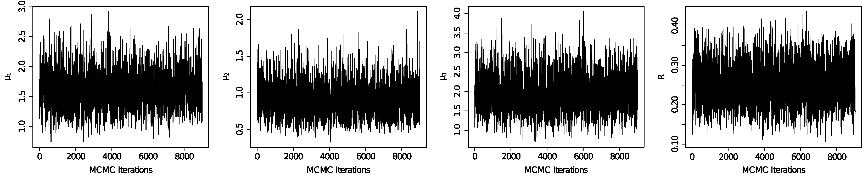
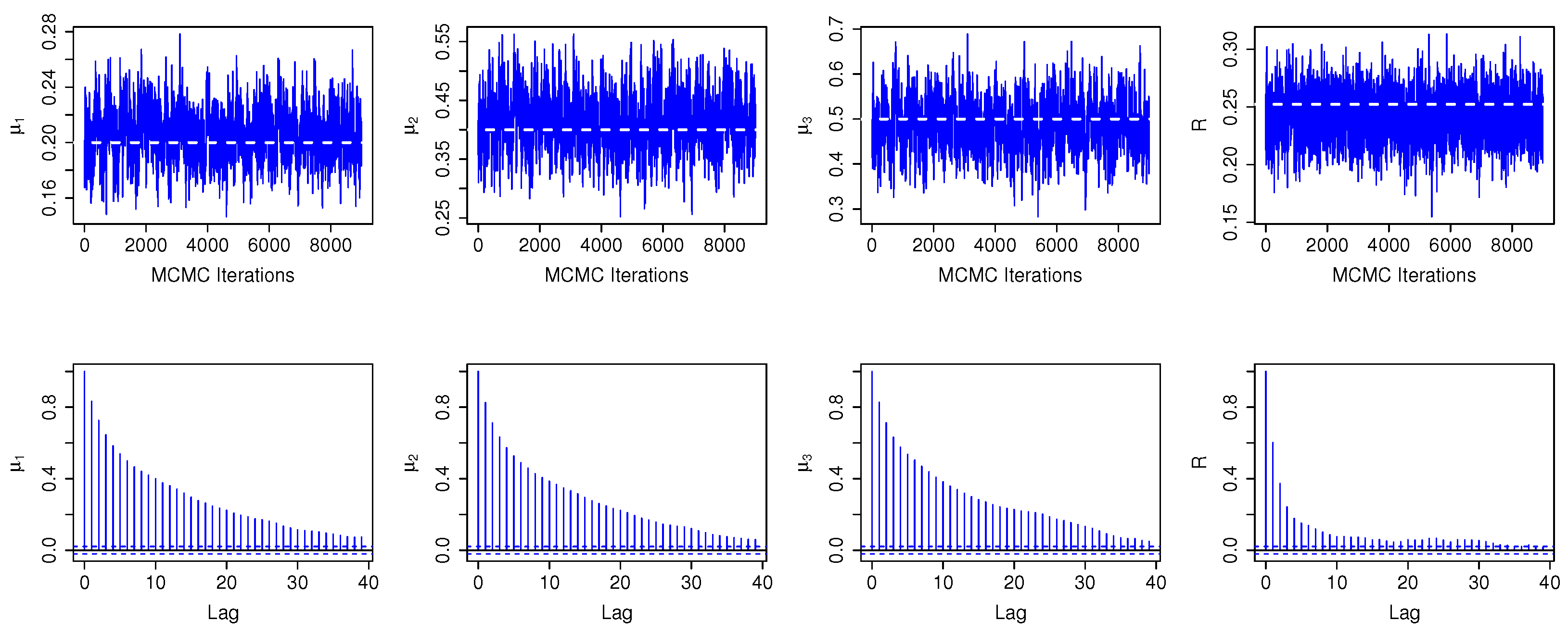
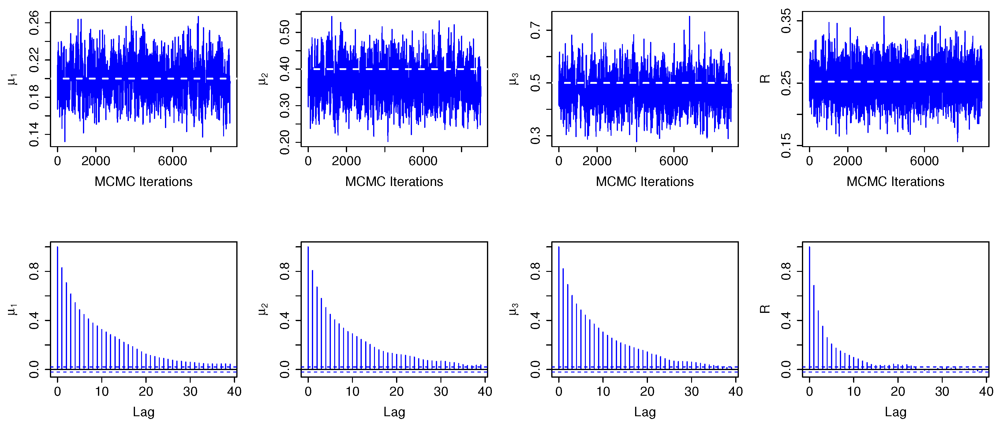
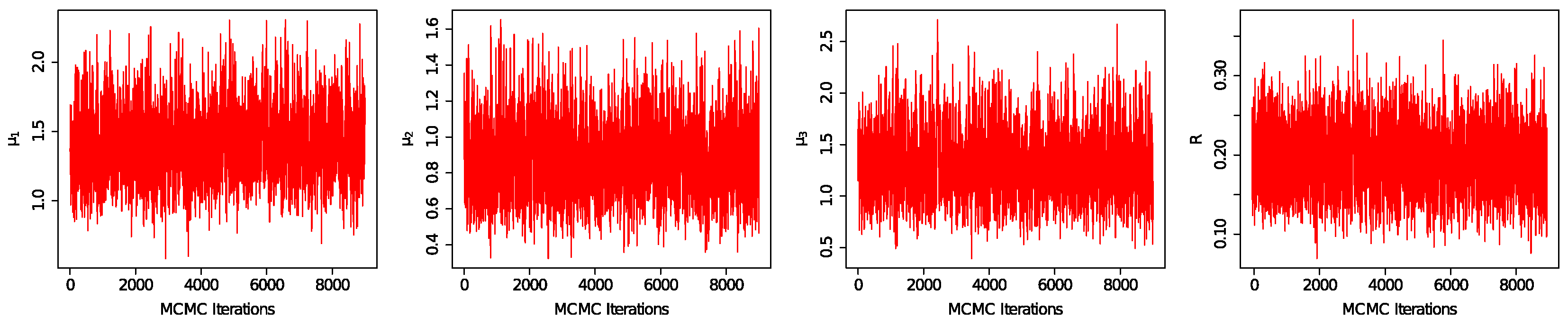
It should be noted that MCMC output analysis is necessary for assessing the convergence of the iteration process in the M-H algorithm, and partial results are presented in Figure 1 and Figure 2 (when n = 100, m = 20; CS = S1 and S2).

Figure 1. The trace and autocorrelation plots of ${\mu }_1,{\mu }_2,{\mu }_3$ and R for MCMC chain based on S1.

Figure 2. The trace and autocorrelation plots of ${\mu }_1,{\mu }_2,{\mu }_3$ and R for MCMC chain based on S2.

All the simulation results of MLE and Bayesian methods are provided from Table 3, Table 4, Table 5 and Table 6.

Table 3. ABs and MSEs (within bracket) for MLE and Bayes point estimation of ${\mu }_1,{\mu }_2$ and ${\mu }_3$.

($\mathit{n},\mathit{m}$)	Scheme	${\widehat{\mathit{\mu }}}_1$		${\widehat{\mathit{\mu }}}_2$		${\widehat{\mathit{\mu }}}_3$
		MLE	Bayesian	MLE	Bayesian	MLE	Bayesian
$\theta =2$
(40, 20)	S1	0.0192 (0.0012)	0.0163 (0.0010)	0.0371 (0.0055)	0.0264 (0.0047)	0.0449 (0.0083)	0.0359 (0.0061)
	S2	0.0072 (0.0008)	0.0030 (0.0007)	0.0145 (0.0033)	0.0033 (0.0032)	0.0198 (0.0059)	0.0121 (0.0062)
(100, 20)	S1	0.0181 (0.0008)	0.0132 (0.0006)	0.0343 (0.0039)	0.0284 (0.0035)	0.0433 (0.0060)	0.0278 (0.0056)
	S2	0.0044 (0.0004)	0.0023 (0.0003)	0.0108 (0.0019)	0.0049 (0.0017)	0.0120 (0.0030)	0.0045 (0.0025)
(100, 40)	S1	0.0172 (0.0006)	0.0225 (0.0008)	0.0324 (0.0027)	0.0414 (0.0035)	0.0379 (0.0040)	0.0488 (0.0055)
	S2	0.0018 (0.0002)	0.0011 (0.0003)	0.0041 (0.0012)	0.0031 (0.0014)	0.0036 (0.0018)	0.0011 (0.0020)
$\theta =3$
(40, 20)	S1	0.0189 (0.0011)	0.0159 (0.0011)	0.0353 (0.0042)	0.0298 (0.0051)	0.0456 (0.0073)	0.0317 (0.0083)
	S2	0.0062 (0.0006)	0.0048 (0.0007)	0.0129 (0.0026)	0.0045 (0.0025)	0.0179 (0.0043)	0.0078 (0.0041)
(100, 20)	S1	0.0170 (0.0008)	0.0158 (0.0007)	0.0326 (0.0035)	0.0310 (0.0031)	0.0416 (0.0055)	0.0354 (0.0043)
	S2	0.0026 (0.0003)	0.0013 (0.0002)	0.0047 (0.0015)	−0.0006 (0.0010)	0.0057 (0.0023)	0.0017 (0.0019)
(100, 40)	S1	0.0151 (0.0005)	0.0102 (0.0002)	0.0286 (0.0023)	0.0124 (0.0002)	0.0354 (0.0036)	0.0020 (0.0001)
	S2	0.0022 (0.0002)	0.0026 (0.0002)	0.0035 (0.0011)	0.0059 (0.0011)	0.0051 (0.0017)	0.0015 (0.0015)
$\theta =4$
(40, 20)	S1	0.0189 (0.0011)	0.0189 (0.0013)	0.0370 (0.0045)	0.0334 (0.0047)	0.0453 (0.0068)	0.0460 (0.0085)
	S2	0.0026 (0.0003)	0.0039 (0.0006)	0.0049 (0.0015)	0.0076 (0.0029)	0.0062 (0.0024)	0.0069 (0.0044)
(100, 20)	S1	0.0165 (0.0008)	0.0141 (0.0007)	0.0319 (0.0032)	0.0243 (0.0028)	0.0399 (0.0051)	0.0308 (0.0043)
	S2	0.0026 (0.0003)	−0.0006 (0.0004)	0.0049 (0.0015)	−0.0023 (0.0020)	0.0062 (0.0024)	0.0001 (0.0029)
(100, 40)	S1	0.0143 (0.0005)	0.0106 (0.0003)	0.0268 (0.0020)	0.0192 (0.0013)	0.0334 (0.0031)	0.0232 (0.0022)
	S2	0.0021 (0.0002)	−0.0008 (0.0002)	0.0042 (0.0010)	−0.0020 (0.0009)	0.0053 (0.0015)	0.0003 (0.0015)
$\theta =5$
(40, 20)	S1	0.0194 (0.0011)	0.0190 (0.0010)	0.0367 (0.0046)	0.0343 (0.0033)	0.0462 (0.0073)	0.0458 (0.0059)
	S2	0.0055 (0.0006)	0.0032 (0.0005)	0.0114 (0.0025)	0.0061 (0.0019)	0.0127 (0.0038)	0.0105 (0.0030)
(100, 20)	S1	0.0161 (0.0008)	0.0161 (0.0007)	0.0320 (0.0032)	0.0313 (0.0027)	0.0395 (0.0050)	0.0413 (0.0043)
	S2	0.0030 (0.0004)	0.0055 (0.0004)	0.0061 (0.0016)	0.0094 (0.0017)	0.0072 (0.0024)	0.0113 (0.0025)
(100, 40)	S1	0.0150 (0.0006)	0.0102 (0.0003)	0.0286 (0.0023)	0.0165 (0.0013)	0.0364 (0.0035)	0.0246 (0.0005)
	S2	0.0015 (0.0002)	0.0012 (0.0005)	0.0028 (0.0010)	0.0017 (0.0002)	0.0026 (0.0016)	0.0014 (0.0010)

Table 4. ABs and MSEs (within bracket) for MLE and Bayes point estimation of R.

($\mathit{n},\mathit{m}$)	Method		$\mathit{\theta }=2$	$\mathit{\theta }=3$	$\mathit{\theta }=4$	$\mathit{\theta }=5$
$(40,20)$	MLE	S1	0.0056 (0.0005)	0.0060 (0.0004)	0.0044 (0.0002)	0.0046 (0.0002)
		S2	0.0029 (0.0005)	0.0026 (0.0003)	0.0026 (0.0002)	0.0026 (0.0003)
	Bayesian	S1	0.0062 (0.0006)	0.0009 (0.0005)	0.0063 (0.0003)	0.0057 (0.0003)
		S2	0.0035 (0.0005)	0.0014 (0.0003)	−0.0011 (0.0002)	0.0020 (0.0001)
$(100,20)$	MLE	S1	0.0061 (0.0003)	0.0053 (0.0002)	0.0043 (0.0001)	0.0035 (0.0001)
		S2	0.0009 (0.0002)	0.0005 (0.0001)	0.0009 (0.0002)	0.0002 (0.0001)
	Bayesian	S1	0.0008 (0.0004)	0.0010 (0.0002)	0.0034 (0.0001)	0.0049 (0.0001)
		S2	−0.0003 (0.0003)	0.0029 (0.0002)	0.0009 (0.0001)	0.0007 (0.0001)
$(100,40)$	MLE	S1	0.0045 (0.0002)	0.0044 (0.0001)	0.0038 (0.0001)	0.0040 (0.0001)
		S2	−0.0001 (0.0001)	0.0007 (0.0001)	0.0004 (0.0001)	−0.0003 (0.0001)
	Bayesian	S1	0.0058 (0.0003)	0.0042 (0.0002)	0.0022 (0.0001)	0.0018 (0.0001)
		S2	−0.0012 (0.0002)	−0.0025 (0.0001)	0.0010 (0.0001)	0.0012 (0.0002)

Table 5. ILs and CPs (within bracket) for MLE and Bayes point estimation of ${\mu }_1,{\mu }_2$ and ${\mu }_3$.

($\mathit{n},\mathit{m}$)	Scheme	${\widehat{\mathit{\mu }}}_1$		${\widehat{\mathit{\mu }}}_2$		${\widehat{\mathit{\mu }}}_3$
		MLE	Bayesian	MLE	Bayesian	MLE	Bayesian
$\theta =2$
(40, 20)	S1	0.1043 (0.8760)	0.0989 (0.9400)	0.2247 (0.8640)	0.2125 (0.9100)	0.2798 (0.8790)	0.2673 (0.9400)
	S2	0.0977 (0.9250)	0.0915 (0.9100)	0.2090 (0.9400)	0.1950 (0.9100)	0.2620 (0.9130)	0.2483 (0.9300)
(100, 20)	S1	0.0825 (0.8590)	0.0759 (0.9000)	0.1846 (0.8610)	0.1746 (0.8900)	0.2308 (0.8600)	0.2155 (0.8900)
	S2	0.0705 (0.9390)	0.0664 (0.9500)	0.1597 (0.9380)	0.1509 (0.9500)	0.1991 (0.9440)	0.1883 (0.9600)
(100, 40)	S1	0.0680 (0.8180)	0.0666 (0.7500)	0.1481 (0.8420)	0.1444 (0.8000)	0.1840 (0.8600)	0.1809 (0.8100)
	S2	0.0616 (0.9520)	0.0585 (0.8900)	0.1340 (0.9380)	0.1275 (0.9100)	0.1669 (0.9500)	0.1586 (0.9400)
$\theta =3$
(40, 20)	S1	0.1000 (0.8780)	0.0935 (0.9100)	0.2071 (0.8950)	0.1954 (0.8800)	0.2596 (0.8880)	0.2423 (0.8400)
	S2	0.0902 (0.9350)	0.0856 (0.8800)	0.1875 (0.9230)	0.1761 (0.9500)	0.2350 (0.9240)	0.2215 (0.9200)
(100, 20)	S1	0.0811 (0.8580)	0.0760 (0.9000)	0.1720 (0.8610)	0.1622 (0.8700)	0.2152 (0.8600)	0.2015 (0.9200)
	S2	0.0677 (0.9520)	0.0633 (0.9600)	0.1440 (0.9410)	0.1343 (0.9800)	0.1800 (0.9480)	0.1691 (0.9700)
(100, 40)	S1	0.0652 (0.8390)	0.1214 (0.9520)	0.1363 (0.8590)	0.1436 (0.9460)	0.1702 (0.8600)	0.1528 (0.9620)
	S2	0.0578 (0.9450)	0.0546 (0.9300)	0.1207 (0.9420)	0.1149 (0.9400)	0.1511 (0.9340)	0.1420 (0.9300)
$\theta =4$
(40, 20)	S1	0.0984 (0.8620)	0.0920 (0.8400)	0.2011 (0.8660)	0.1877 (0.8500)	0.2510 (0.8780)	0.2371 (0.7800)
	S2	0.0670 (0.9300)	0.0813 (0.9100)	0.1391 (0.9290)	0.1673 (0.9100)	0.1739 (0.9280)	0.2080 (0.8900)
(100, 20)	S1	0.0808 (0.8410)	0.0739 (0.8300)	0.1670 (0.8650)	0.1526 (0.8600)	0.2089 (0.8500)	0.1914 (0.8600)
	S2	0.0670 (0.9300)	0.0618 (0.8900)	0.1391 (0.9290)	0.1285 (0.8800)	0.1739 (0.9280)	0.1616 (0.8700)
(100, 40)	S1	0.0644 (0.8470)	0.0594 (0.9400)	0.1319 (0.8610)	0.1217 (0.9300)	0.1648 (0.8640)	0.1525 (0.9100)
	S2	0.0560 (0.9330)	0.0511 (0.9100)	0.1152 (0.9370)	0.1048 (0.8900)	0.1440 (0.9310)	0.1319 (0.9000)
$\theta =5$
(40, 20)	S1	0.0978 (0.8500)	0.0922 (0.9100)	0.1979 (0.8570)	0.1865 (0.9300)	0.2475 (0.8550)	0.2343 (0.9000)
	S2	0.0846 (0.9310)	0.0805 (0.9000)	0.1722 (0.9220)	0.1640 (0.9100)	0.2146 (0.9290)	0.2059 (0.9200)
(100, 20)	S1	0.0804 (0.8560)	0.0747 (0.8700)	0.1647 (0.8450)	0.1532 (0.8900)	0.2057 (0.8630)	0.1918 (0.8900)
	S2	0.0670 (0.9210)	0.0636 (0.8800)	0.1374 (0.9230)	0.1303 (0.8800)	0.1717 (0.9230)	0.1627 (0.8900)
(100, 40)	S1	0.0644 (0.8310)	0.1205 (0.9300)	0.1307 (0.8300)	0.1036 (0.9200)	0.1636 (0.8240)	0.1545 (0.8500)
	S2	0.0550 (0.9300)	0.0423 (0.8512)	0.1121 (0.9190)	0.0325 (0.8400)	0.1399 (0.9160)	0.0256 (0.9300)

Table 6. ILs and CPs (within bracket) for MLE and Bayes point estimation of R.

($\mathit{n},\mathit{m}$)	Method		$\mathit{\theta }=2$	$\mathit{\theta }=3$	$\mathit{\theta }=4$	$\mathit{\theta }=5$
$(40,20)$	ACI	S1	0.1318 (0.9920)	0.0960 (0.9870)	0.0744 (0.9860)	0.0627 (0.9740)
		S2	0.1214 (0.9870)	0.0866 (0.9890)	0.0691 (0.9790)	0.0567 (0.9670)
	HPD	S1	0.0703 (0.8800)	0.0561 (0.8300)	0.0475 (0.8300)	0.0422 (0.8400)
		S2	0.0663 (0.8200)	0.0534 (0.9200)	0.0450 (0.8900)	0.0396 (0.9200)
$(100,20)$	ACI	S1	0.1019 (0.9950)	0.0730 (0.9900)	0.0561 (0.9770)	0.0468 (0.9630)
		S2	0.0876 (0.9920)	0.0613 (0.9820)	0.0876 (0.9920)	0.0399 (0.9680)
	HPD	S1	0.0549 (0.8000)	0.0386 (0.8900)	0.0359 (0.8900)	0.0312 (0.8900)
		S2	0.0481 (0.8700)	0.0431 (0.8800)	0.0328 (0.8700)	0.0282 (0.8800)
$(100,40)$	ACI	S1	0.0855 (0.9960)	0.0613 (0.9820)	0.0481 (0.9800)	0.0400 (0.9690)
		S2	0.0756 (0.9910)	0.0545 (0.9830)	0.0431 (0.9780)	0.0353 (0.9720)
	HPD	S1	0.0450 (0.8400)	0.0386 (0.8700)	0.0311 (0.9100)	0.0235 (0.9200)
		S2	0.0417 (0.8500)	0.0337 (0.8300)	0.0280 (0.8400)	0.0154 (0.9500)

It can be seen from Table 3 and Table 4 that when the dependent parameters and the censored scheme are given time, the deviation and MSE of the maximum likelihood estimation and Bayes estimation of the model parameters and reliability R gradually decrease with the increase in sample n. When the sample, dependent parameters, and censored scheme are given time, the Bayesian estimation results are better than the maximum likelihood estimation. When the sample and the censored scheme are given, the model parameters and reliability R do not change significantly with the increase in the dependent parameters. When samples and dependent parameters are given, the estimated values of parameters and reliability under scheme S2 are significantly better than those under censored S1, which provides suggestions for our actual data analysis.

As can be seen from Table 5 and Table 6, when the dependent parameters and censored scheme are given, ACI and IL of HPD CIs of model parameters and reliability R gradually decrease with the increase in the sample size, but CP changes are not obvious. When samples, dependent parameters and censored schemes are given, the IL of HPD CIs is smaller than that of ACI. When the sample and the censored scheme are given, the IL of the model parameters and reliability R interval estimation decreases with the increase in the dependent parameters. When samples and dependent parameters are given, the interval IL of parameters and reliability estimated in scheme S2 is significantly smaller than that in scheme S1, but CP changes insignificantly.

Through the above analysis, it is found that better estimation results can be obtained by using Bayesian estimation under the S2.

5. Real Data Application

In this section, we conduct a practical investigation using three actual datasets. Data 1 and Data 2 were examined by [42] for stress–strength reliability analysis and Data 3 was explored by [43] for stress–strength reliability estimations. All the datasets underwent analysis conducted by [44]. In this instance, the three datasets serve as illustrative examples of the aforementioned techniques. The specific details of these four datasets are outlined below.

Data 1: 693.73, 704.66, 323.83, 778.17, 123.06, 637.66, 383.43, 151.48, 108.94, 50.16, 671.49, 183.16, 727.23, 257.44, 291.27, 101.15, 376.42, 163.40, 141.38, 700.74, 262.90, 353.24, 422.11, 43.93, 590.48, 212.13, 303.90, 506.60, 530.55, 177.25

Data 2: 71.46, 419.02, 284.64, 585.57, 456.60, 688.16, 662.66, 113.85, 187.85, 45.58, 578.62, 756.70, 594.29, 166.49, 707.36, 99.72, 765.14, 187.13, 145.96, 350.70, 547.44, 116.99, 375.81, 119.86, 581.60, 48.01, 200.16, 36.75, 244.53, 83.55

Data 3: 6.53, 7, 10.42, 14.48, 16, 10, 22.70, 34, 41.55, 42, 45.28, 49.40, 53.62, 63, 83, 84, 91, 108, 112, 129, 133, 133, 139, 140, 140, 146, 149, 154, 157, 160, 160, 165, 173, 176, 218, 225, 241, 248, 273, 277, 297, 405, 417, 420, 440, 523, 583, 594, 1101, 1146, 1417

To ensure a more efficient analysis of dependencies, it is crucial to maintain a uniform sample size across all datasets. Currently, the sample sizes for Data 1 and Data 2 are both 30, while those for Data 3 exceed this number. To address this issue, we utilized the ’sample()’ function in R to randomly select two sets of 30 data points each from Data 3, which were labeled as Data^∗3.

Data^∗3: 173.00, 16.00, 140.00, 49.40, 22.70, 133.00, 146.00, 273.00, 583.00, 112.00, 523.00, 277.00, 241.00, 10.42, 42.00, 176.00, 218.00, 1417.00, 417.00, 14.48, 140.00, 1146.00, 594.00, 297.00, 53.62, 154.00, 10.00, 7.00, 165.00, 45.28

Without loss of generality, let Data 1 represent stress $Y_1$, Data 2 represent strength X, and Data^∗3 represent stress $Y_2$. For ease of calculation, all the data are divided by 1000, and sorted by COS; the transformed complete data are as follows in Table 7.

Table 7. Complete data sets.

X	0.03675	0.04558	0.04801	0.07146	0.08355	0.09972	0.11385	0.11699
	0.11986	0.14596	0.16649	0.18713	0.18785	0.20016	0.24453	0.28464
	0.35070	0.37581	0.41902	0.45660	0.54744	0.57862	0.58160	0.58557
	0.59429	0.66266	0.68816	0.70736	0.75670	0.76514
$Y_1$	0.00700	0.11200	0.15400	0.17300	0.04528	0.17600	0.27300	1.14600
	0.29700	0.41700	0.01042	1.41700	0.58300	0.01000	0.16500	0.14000
	0.01448	0.59400	0.01600	0.02270	0.14000	0.52300	0.05362	0.04940
	0.24100	0.14600	0.13300	0.04200	0.27700	0.21800
$Y_2$	0.50660	0.05016	0.21213	0.69373	0.17725	0.10115	0.15148	0.35324
	0.04393	0.14138	0.25744	0.16340	0.10894	0.30390	0.53055	0.32383
	0.70074	0.42211	0.70466	0.12306	0.26290	0.67149	0.59048	0.77817
	0.72723	0.38343	0.63766	0.29127	0.18316	0.37642

Assuming that X follows the PRHR model with distribution function $F^{{\mu }_1}\left(x\right)$, $Y_1$ follows the PRHR model with distribution function $F^{{\mu }_2}\left(x\right)$, and $Y_2$ follows the PRHR model with distribution function $F^{{\mu }_3}\left(x\right)$, where the baseline distribution is given by $F\left(x\right)=1-exp(-3.5x)$.

First, it was checked whether the PRHR model can be used or not to analyze the three data sets separately. With the estimated parameters, for X, $Y_1$ and $Y_2$, the Kolmogorov–Smirnov statistics and the corresponding p-value and AD statistics and the corresponding p-value are given in Table 8; the empirical distribution functions are given in Figure 3. The p-value indicates that the PRHR model adequately fits these data sets.

Table 8. Results of the K-S test and AD test for the real data.

	${\widehat{\mathit{\mu }}}_1$	${\widehat{\mathit{\mu }}}_2$	${\widehat{\mathit{\mu }}}_3$	KS	p-Value	AD	p-Value
X	1.5060	-	-	0.1201	0.7650	0.6201	0.6277
$Y_1$	-	0.7718	-	0.0996	0.9270	0.3849	0.8625
$Y_2$	-	-	1.8114	0.1157	0.7743	0.4008	0.8468

Figure 3. Comparative plots of the empirical distribution of the sample data and the fitted distribution of real data sets.

By employing the moment method (Section 3.1), we determine that the dependent parameter $\theta$ for $X,Y_1,Y_2$ is estimated as $\widehat{\theta }=0.1184$. Furthermore, we utilize a goodness-of-fit test for copula to discern the dependence structure between X, $Y_1$, and $Y_2$. This test is rooted in the multiplier central limit theorems and was introduced by [45]. We present the goodness-of-fit test results for Clayton, Gumbel and Frank copula applied to X and $Y_1$ and $Y_2$ in Table 9. The p-value indicates that the Clayton copula provides an adequate fit for the dependence of these data sets.

Table 9. Goodness-of-fit test for copula.

	Clayton	Gumbel	Frank
statistic	0.0349	0.0576	0.0533
p-value	0.5099	0.2129	0.1337

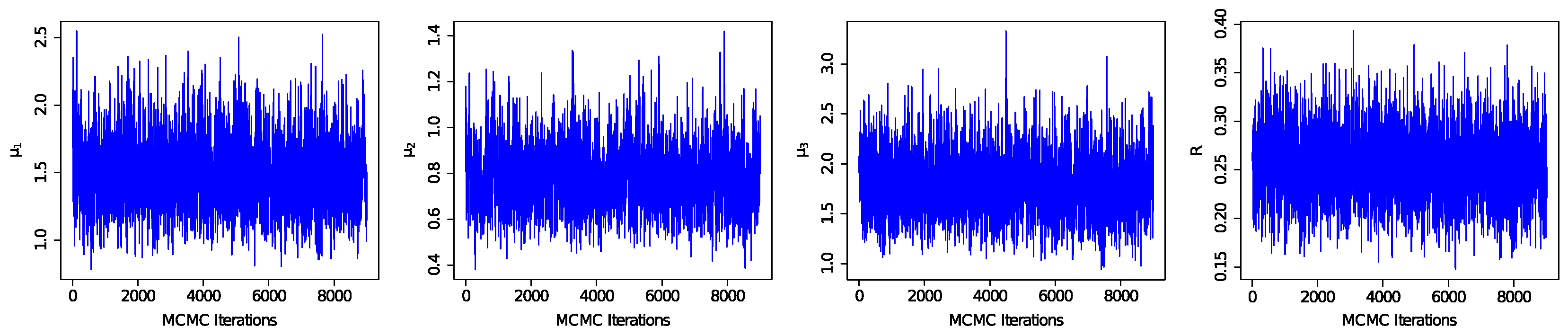
Based on complete data sets (Table 7), the MLEs and Bayesian estimator and 95% ACIs and HPD CIs of ${\mu }_1,{\mu }_2,{\mu }_3$ and R are given in Table 10, and trace plots are given in Figure 4. As can be seen from Figure 4, the estimated value has good convergence and stability.

Table 10. Estimate results of ${\mu }_1,{\mu }_2,{\mu }_3$ and R based on complete data sets.

	${\widehat{\mathit{\mu }}}_1$	${\widehat{\mathit{\mu }}}_2$	${\widehat{\mathit{\mu }}}_3$	$\widehat{\mathit{R}}$
MLE	1.5060	0.7718	1.8114	0.2593
Bayesian	1.5035	0.7867	1.7995	0.2559
ACI	(1.0562, 2.1472)	(0.5410, 1.1010)	(1.2703, 2.5832)	(0, 0.7127)
HPD	(0.9771, 2.0248)	(0.5328, 1.0842)	(1.1715, 2.4180)	(0.1971, 0.3020)

Figure 4. The trail plots of ${\widehat{\mu }}_1$, ${\widehat{\mu }}_2$, ${\widehat{\mu }}_3$ and $\widehat{R}$ under complete sample.

For illustrative purposes, two different progressive type II censored samples have been generated from the above sets:

$$S1:(0\ast 7,n-m,0\ast 7),and,S2:(0\ast (m-1),n-m).$$

Based on schemes $S1$ and $S2,$ the data sets are as follows in Table 11 and Table 12, respectively. The MLEs and Bayesian estimator and 95% ACIs and HPD CIs of ${\mu }_1,{\mu }_2,{\mu }_3$ and R are given in Table 13, and trace plots are given in Figure 5 and Figure 6, respectively. As can be seen from Figure 5 and Figure 6, the estimated value has good convergence and stability. By comparing the complete sample and $S1$ and $S2$, it is easy to find that the estimated results of scheme $S1$ are very close to the complete sample.

Table 11. Censored data sets under $S1$.

X	0.03675	0.04558	0.04801	0.07146	0.08355	0.09972	0.11385	0.11699
	0.58557	0.59429	0.66266	0.68816	0.70736	0.75670	0.76514
$Y_1$	0.00700	0.11200	0.15400	0.17300	0.04528	0.17600	0.27300	1.14600
	0.04940	0.24100	0.14600	0.13300	0.04200	0.27700	0.21800
$Y_2$	0.50660	0.05016	0.21213	0.69373	0.17725	0.10115	0.15148	0.35324
	0.77817	0.72723	0.38343	0.63766	0.29127	0.18316	0.37642

Table 12. Censored data sets under $S2$.

X	0.03675	0.04558	0.04801	0.07146	0.08355	0.09972	0.11385	0.11699
	0.11986	0.14596	0.16649	0.18713	0.18785	0.20016	0.24453
$Y_1$	0.00700	0.11200	0.15400	0.17300	0.04528	0.17600	0.27300	1.14600
	0.29700	0.41700	0.01042	1.41700	0.58300	0.01000	0.16500
$Y_2$	0.50660	0.05016	0.21213	0.69373	0.17725	0.10115	0.15148	0.35324
	0.04393	0.14138	0.25744	0.16340	0.10894	0.30390	0.53055

Table 13. Estimate results of ${\mu }_1,{\mu }_2,{\mu }_3$ and R based on progressive type II censored data sets.

Scheme		${\widehat{\mathit{\mu }}}_1$	${\widehat{\mathit{\mu }}}_2$	${\widehat{\mathit{\mu }}}_3$	$\widehat{\mathit{R}}$
MLE	$S1$	1.6394	0.9155	1.9865	0.2579
	$S2$	1.4159	0.8687	1.3142	0.1953
Bayesian	$S1$	1.6242	0.9300	1.9563	0.2579
	$S2$	1.4068	0.8793	1.3084	0.1952
ACI	$S1$	(1.1249, 2.3894)	(0.5549, 1.5104)	(1.2065, 3.2707)	(0, 0.9555)
	$S2$	(0.9864, 2.0323)	(0.5275, 1.4303)	(0.7956, 2.1706)	(0, 0.5896)
HPD	$S1$	(1.0167, 2.2383)	(0.4821, 1.3829)	(1.0642, 2.9352)	(0.1742, 0.3185)
	$S2$	(0.9048, 1.9051)	(0.4896, 1.3326)	(0.6759, 1.9447)	(0.1276, 0.2478)

Figure 5. The trail plots of ${\widehat{\mu }}_1$, ${\widehat{\mu }}_2$, ${\widehat{\mu }}_3$ and $\widehat{R}$ under scheme $S1$.

Figure 6. The trail plots of ${\widehat{\mu }}_1$, ${\widehat{\mu }}_2$, ${\widehat{\mu }}_3$ and $\widehat{R}$ under sample $S2$.

6. Conclusions

In this paper, the problem of statistical analysis and reliability evaluation of the product-dependent stress–strength model with double stress is deeply studied. In this model, the dependent structure is described by a 3-dimensional Clayton copula function, with marginal distributions selected from the PRHR model. By employing a progressive Type II censoring scheme, we obtained MLE and Bayesian estimates for the model parameters and reliability. The simulation results indicate that both sample size and censoring scheme significantly impact the outcomes, with Bayesian estimation outperforming MLE. The real data analysis further proves that the model can be successfully applied to the statistical modeling analysis of real data.

In the field of reliability engineering, the utilization of this model enhances the comprehension of system and product performance behaviors, improves the accuracy of reliability predictions, and provides robust quantitative foundations for decision-making, which is an indispensable aspect in achieving high-quality, high-performance, and cost-effective engineering practices. In medical applications, this model holds great potential to assist doctors in comprehending the probability of treatment effectiveness, enabling more scientifically informed clinical decisions and ultimately enhancing the efficiency and effectiveness of medical interventions. Through our study outlined in this article, we have identified that defining the research problem accurately is crucial for practical applications; furthermore, it is essential to identify key random variables X and determine the scope of interest $(Y_1,Y_2)$. Subsequently, correct distributional assumptions along with parameter estimation based on the analysis of collected sample data are made to establish a statistical model. Finally, inference is performed on the established model which leads to appropriate formulation or adjustment strategies based on inferred results.

This study solely focused on the dual-stress–strength model of a single component; however, with the development of society and the progress of science and technology, the complexity of products and the diversity of services have led to the emergence of more and more complex systems, most of which are multi-component systems. Therefore, how to study the reliability of multi-component systems has become a topic of wide concern. In the follow-up study, we will consider the reliability evaluation of the multi-component dual stress strength model. As pointed out by the reviewers, the M-H algorithm has the problem of insufficient convergence in the case of high dimensions, so in future research, we will explore the updated method.

References

- Nadarajah, S. Reliability for some bivariate gamma distributions. Math. Probl. Eng. 2005, 2005, 151–163. [Google Scholar] [CrossRef]
- Jeevanand, E. Bayes estimation of P(X2<X1) for a bivariate Pareto distribution. J. R. Stat. Soc. Ser. D Stat. 1997, 46, 93–99. [Google Scholar]
- Kotz, S.; Lumelskii, Y.; Pensky, M. The Stress–Strength Model and Its Generalizations: Theory and Applications; World Scientific: Singapore, 2003. [Google Scholar]
- Nadarajah, S.; Kotz, S. Reliability for some bivariate exponential distributions. Math. Probl. Eng. 2006, 2006, 041652. [Google Scholar] [CrossRef]
- Khodadadian, A.; Noii, N.; Parvizi, M.; Abbaszadeh, M.; Wick, T.; Heitzinger, C. A Bayesian estimation method for variational phase-field fracture problems. Comput. Mech. 2020, 66, 827–849. [Google Scholar] [CrossRef] [PubMed]
- Baklizi, A. Bayesian inference for P(Y<X) in the exponential distribution based on records. Appl. Math. Model. 2014, 38, 1698–1709. [Google Scholar]
- Kundu, D.; Gupta, R.D. Estimation of P(Y<X) for Weibull distributions. IEEE Trans. Reliab. 2006, 55, 270–280. [Google Scholar]
- Lio, Y.; Tsai, T.R. Estimation of δ=P(X<Y) for Burr XII distribution based on the progressively first failure-censored samples. J. Appl. Stat. 2012, 39, 309–322. [Google Scholar]
- Al-Mutairi, D.; Ghitany, M.; Kundu, D. Inferences on stress-strength reliability from Lindley distributions. Commun. Stat.-Theory Methods 2013, 42, 1443–1463. [Google Scholar] [CrossRef]
- Nadar, M.; Kızılaslan, F.; Papadopoulos, A. Classical and Bayesian estimation of P(Y<X) for Kumaraswamy’s distribution. J. Stat. Comput. Simul. 2014, 84, 1505–1529. [Google Scholar]
- Bai, X.; Shi, Y.; Liu, Y.; Liu, B. Reliability inference of stress–strength model for the truncated proportional hazard rate distribution under progressively Type-II censored samples. Appl. Math. Model. 2019, 65, 377–389. [Google Scholar] [CrossRef]
- de la Cruz, R.; Salinas, H.S.; Meza, C. Reliability Estimation for Stress-Strength Model Based on Unit-Half-Normal Distribution. Symmetry 2022, 14, 837. [Google Scholar] [CrossRef]
- Yousef, M.M.; Fayomi, A.; Almetwally, E.M. Simulation Techniques for Strength Component Partially Accelerated to Analyze Stress-Strength Model. Symmetry 2023, 15, 1183. [Google Scholar] [CrossRef]
- Wang, M.; Ye, C.; Xu, D. Estimation of structural reliability relative to a dependent bivariate Weibull distribution. Chin. J. Appl. Probab. Stat. 2005, 22, 127–136. [Google Scholar]
- SenGupta, A. Random stress-dependent strength models through bivariate exponential conditionals distributions. In Advances in Distribution Theory, Order Statistics, and Inference; Birkhäuser: Boston, MA, USA, 2006; pp. 327–339. [Google Scholar]
- Gupta, R.C.; Ghitany, M.; Al-Mutairi, D. Estimation of reliability from a bivariate log-normal data. J. Stat. Comput. Simul. 2013, 83, 1068–1081. [Google Scholar] [CrossRef]
- Domma, F.; Giordano, S. Dependence in stress-strength models with FGM copula and Burr III margins. In Book of Short Papers of the Meeting of the Classification and Data Analysis Group of the Italian Statistical Society; CLEUP: Catania, Italy, 2009; pp. 477–480. [Google Scholar]
- Domma, F.; Giordano, S. A stress–strength model with dependent variables to measure household financial fragility. Stat. Methods Appl. 2012, 21, 375–389. [Google Scholar] [CrossRef]
- James, A.; Chandra, N.; Sebastian, N. Stress-strength reliability estimation for bivariate copula function with rayleigh marginals. Int. J. Syst. Assur. Eng. Manag. 2023, 14, 196–215. [Google Scholar] [CrossRef]
- Chandra, S.; Owen, D.B. On estimating the reliability of a component subject to several different stresses (strengths). Nav. Res. Logist. Q. 1975, 22, 31–39. [Google Scholar] [CrossRef]
- Singh, N. On the estimation of Pr (X1 < Y < X2). Commun. Stat.-Theory Methods 1980, 9, 1551–1561. [Google Scholar]
- Dutta, K.; Sriwastav, G. An n-standby system with P (X < Y < Z). IAPQR Trans. 1986, 12, 95–97. [Google Scholar]
- Ivshin, V. On the estimation of the probabilities of a double linear inequality in the case of uniform and two-parameter exponential distributions. J. Math. Sci. 1998, 88, 819–827. [Google Scholar] [CrossRef]
- Patowary, A.; Sriwastav, G.; Hazarika, J. Inference of R = P (X < Y < Z) for n-Standby System: A Monte-Carlo Simulation Approach. J. Math 2016, 12, 18–22. [Google Scholar]
- Emura, T.; Konno, Y. Multivariate normal distribution approaches for dependently truncated data. Stat. Pap. 2012, 53, 133–149. [Google Scholar] [CrossRef]
- Burcu, H.; Selim, Orhun, S. On the copula-based reliability of stress-strength model under bivariate stress. Int. J. Gen. Syst. 2023, 52, 842–863. [Google Scholar]
- Joe, H. Multivariate Models and Multivariate Dependence Concepts; CRC Press: Boca Raton, FL, USA, 1997. [Google Scholar]
- Nelsen, R.B. An Introduction to Copulas; Springer: New York, NY, USA, 2006. [Google Scholar]
- Durante, F.; Sempi, C. Copula theory and its applications. In Proceedings of the Workshop, Warsaw, Poland, 25–26 September 2009; pp. 25–26. [Google Scholar]
- Ramesh, C. Gupta, P.L.G.; Gupta, R.D. Modeling failure time data by lehman alternatives. Commun. Stat.—Theory Methods 1998, 27, 887–904. [Google Scholar]
- David, H.A.; Nagaraja, H.N. Concomitants of order statistics. Handb. Stat. 1998, 16, 487–513. [Google Scholar]
- Alotaibi, R.; Almetwally, E.M.; Kumar, D.; Rezk, H. Optimal test plan of step-stress model of alpha power Weibull lifetimes under progressively type-II censored samples. Symmetry 2022, 14, 1801. [Google Scholar] [CrossRef]
- Haj Ahmad, H.; Elnagar, K.; Ramadan, D. Investigating the Lifetime Performance Index under Ishita Distribution Based on Progressive Type II Censored Data with Applications. Symmetry 2023, 15, 1779. [Google Scholar] [CrossRef]
- Ghazal, M.G.; Hasaballah, M.M.; EL-Sagheer, R.M.; Balogun, O.S.; Bakr, M.E. Bayesian Analysis Using Joint Progressive Type-II Censoring Scheme. Symmetry 2023, 15, 1884. [Google Scholar] [CrossRef]
- Akdam, N. Bayes Estimation for the Rayleigh and Weibull Distribution Based on Progressive Type-II Censored Samples for Cancer Data in Medicine. Symmetry 2022, 15, 1754. [Google Scholar] [CrossRef]
- Balakrishnan, N.; Kim, J.A. Point and interval estimation for bivariate normal distribution based on progressively Type-II censored data. Commun. Stat.—Theory Methods 2005, 34, 1297–1347. [Google Scholar] [CrossRef]
- Oehlert, G.W. A note on the delta method. Am. Stat. 1992, 46, 27–29. [Google Scholar]
- Wasserman, L. All of Statistics: A Concise Course in Statistical Inference; Springer: New York, NY, USA, 2004; Volume 26. [Google Scholar]
- Peña, E.A.; Gupta, A.K. Bayes estimation for the Marshall–Olkin exponential distribution. J. R. Stat. Soc. Ser. B Stat. Methodol. 1990, 52, 379–389. [Google Scholar] [CrossRef]
- Noii, N.; Khodadadian, A.; Ulloa, J.; Aldakheel, F.; Wick, T.; Francois, S.; Wriggers, P. Bayesian inversion with open-source codes for various one-dimensional model problems in computational mechanics. Arch. Comput. Methods Eng. 2022, 29, 4285–4318. [Google Scholar] [CrossRef]
- Congdon, P. Applied Bayesian Modelling; John Wiley & Sons: New York, NY, USA, 2003. [Google Scholar]
- Saraçoğlu, B.; Kinaci, I.; Kundu, D. On estimation of R=P(Y<X) for exponential distribution under progressive type-II censoring. J. Stat. Comput. Simul. 2012, 82, 729–744. [Google Scholar]
- Iranmanesh, A.; Fathi Vajargah, K.; Hasanzadeh, M. On the estimation of stress strength reliability parameter of inverted gamma distribution. Math. Sci. 2018, 12, 71–77. [Google Scholar] [CrossRef]
- Bai, X.; Li, X.; Balakrishnan, N.; He, M. Statistical inference for dependent stress–strength reliability of multi-state system using generalized survival signature. J. Comput. Appl. Math. 2021, 390, 113316. [Google Scholar] [CrossRef]
- Kojadinovic, I.; Yan, J. A goodness-of-fit test for multivariate multiparameter copulas based on multiplier central limit theorems. Stat. Comput. 2011, 21, 17–30. [Google Scholar] [CrossRef]
Disclaimer/Publisher’s Note: The statements, opinions and data contained in all publications are solely those of the individual author(s) and contributor(s) and not of MDPI and/or the editor(s). MDPI and/or the editor(s) disclaim responsibility for any injury to people or property resulting from any ideas, methods, instructions or products referred to in the content. |
© 2024 by the authors. Licensee MDPI, Basel, Switzerland. This article is an open access article distributed under the terms and conditions of the Creative Commons Attribution (CC BY) license (https://creativecommons.org/licenses/by/4.0/).