Exponentiated Generalized Xgamma Distribution Based on Dual Generalized Order Statistics: A Bayesian and Maximum Likelihood Approach

Abstract

In this paper the exponentiated generalized xgamma distribution is introduced. Some of its properties are presented through some models of stress–strength, moments, mean residual life, mean past lifetime, and order statistics. The maximum likelihood estimators, confidence intervals for the parameters, and the reliability and the hazard rate functions of the exponentiated generalized xgamma distribution based on dual generalized order statistics are obtained. Bayesian estimators for the unknown parameters, reliability, and hazard rate functions of the exponentiated generalized xgamma distribution based on dual generalized order statistics are considered. The results based on lower record values are verified using simulations as well as three real sets of data are adopted to demonstrate the flexibility and potential applications of the distribution.

1. Introduction

In numerous situations involving life testing and reliability studies, several models of ordered random variables are used, such as order statistics, upper record values, Pfeifer records, and sequential order statistics. These models play an important role in statistics in general and in various fields, like reliability theory, life testing, engineering, hydrology, psychology, medicine, and seismology. The concept of generalized order statistics (gos) was introduced by [1] as a unified approach to encompass various types of ordered random variables, including order statistics, sequential order statistics, records, and Pfeifer records.

However, the traditional framework of generalized order statistics (GOS) is limited to increasingly ordered random variables. To address this limitation, ref. [2] introduced the concept of dual generalized order statistics (dgos), which allows for the study of both increasing and decreasing order statistics. This framework encompasses various types of ordered random variables, including reversed order statistics, lower record values, and lower Pfeifer records. Ref. [3] further developed the theory of dgos and provided a comprehensive framework for analyzing these types of ordered random variables. For practical applications, dgos can be particularly useful when the survival function $1-F\left(x\right)$ is in a closed form. In such cases, dgos provide a flexible and unified approach to analyze the statistical properties of these ordered random variables. For more details about dgos, see [4,5,6,7,8,9,10,11,12].

Lower record values are a statistical concept used to describe the smallest observed values in a sequence of random variables. They represent new minimum values as they occur. Lower record values are crucial in various fields, including reliability theory, meteorology, hydrology, seismology, and mining. They help analyze real-life problems and many situations of daily life, e.g., Olympic records, sports events, weather, rainfall, temperature, flood levels, economics, and the lowest stock markets figure. By studying lower record values, researchers can gain insights into the distribution of extreme events and make predictions about future occurrences (see [13,14]).

Let $X_{\left(1,n,m,k\right)},X_{\left(2,n,m,k\right)},{\dots X}_{\left(n,n,m,k\right)}$ be $n$ dgos from an absolutely cumulative distribution function (cdf) with a corresponding probability density function (pdf). Then, the joint pdf has the following form are

$$f_{X_{\left(1,n,m,k\right)}, X_{\left(2,n,m,k\right)}, {\dots X}_{\left(n,n,m,k\right)} }\left(x_{\left(1\right)},\dots ,x_{\left(n\right)}\right)=k \left(\prod _{j_1=1}^{n-1}{\gamma }_{j_1}\right)\left[\prod _{i=1}^{n-1}{\left(F\left(x_{\left(i\right)}\right)\right)}^{m}f\left(x_{\left(i\right)}\right)\right]{\left(F\left(x_{\left(n\right)}\right)\right)}^{k-1}f\left(x_{\left(n\right)}\right);$$

(1)

where $F^{-1}\left(1\right)\ge x_{\left(1\right)}\dots \ge x_{\left(n\right)}\ge F^{-1}\left(0\right)$, $n\in N, k\ge 1, m_1,\dots ,m_{n-1}=m, m\in R$ are the parameters, such that ${\gamma }_r=k+\left(n-r\right)\left(m+1\right)\ge 1, for all 1\le r\le n.$ The joint pdf of the first n lower record values $X_{L\left(1\right)},X_{L\left(2\right)},\dots ,X_{L\left(n\right)}$, for $m=-1, k=1$ in (1) is given by

$$f^{X_L\left(1\right),\dots ,X_L\left(n\right)}\left(x_{L\left(1\right)},\dots {,x}_{L\left(n\right)}\right)=\left(\prod _{i=1}^{n-1}{\displaystyle \frac{f\left(x_{\left(i\right)}\right)}{F\left(x_{\left(i\right)}\right)}}\right)f\left(x_{\left(n\right)}\right),\hspace{1em}\hspace{1em}{x}_{L\left(1\right)}\ge \cdots \ge x_{L\left(n\right)}$$

(2)

General classes of distributions are important as they provide a unified framework for analyzing a wide range of statistical problems. By studying general classes, one can obtain results that can be applied to specific distributions, leading to greater flexibility and flexibility in statistical modeling. Ref. [15] proposed exponentiated generalized (EG) distributions as an extension of the exponentiated type distribution which have greater flexibility in their tails and can be widely applied in many areas of engineering and biology. Many authors focused on the generalized and EG distributions and their applications. Given a non-negative continuous random variable $X$, the cdf of the EG of distributions is defined by the following Equation (3):

$$F\left(x;\alpha ,\beta \right)={\left[1-{\left\{1-G\left(x\right)\right\}}^{\alpha }\right]}^{\beta },\hspace{1em}x>0,\hspace{1em}\alpha ,\beta >0,$$

(3)

where $\alpha \mathrm{a}\mathrm{n}\mathrm{d} \beta$ are additional shape parameters. The corresponding pdf for (3) is given by

$$f\left(x;\alpha ,\beta \right)=\alpha {\beta g\left(x\right)\left\{1-G\left(x\right)\right\}}^{\alpha -1}{\left[1-{\left\{1-G\left(x\right)\right\}}^{\alpha }\right]}^{\beta -1},\hspace{1em}x>0,\hspace{1em}\hspace{1em}\alpha ,\beta >0,$$

(4)

where $g\left(x\right)$ is the first derivative of $G\left(x\right)$ with respect to $x$. $G\left(x\right)$ represents the cdf of the EG of distributions, is a continuous and non-decreasing function defined on the real line, and its range is the interval [0, 1]. The quantile function of $F\left(x\right)$ has a straightforward form, making it particularly tractable for simulations, where $x=Q_G[1-{(1-u^{{\displaystyle \frac{1}{\beta }}})}^{{\displaystyle \frac{1}{\alpha }}}]$ and $Q_G\left(u\right)$ is the baseline quantile function.

By setting $\alpha =1 \mathrm{i}\mathrm{n} \left(4\right)$ the exponentiated type distribution is derived by [16]; furthermore, the exponentiated exponential and exponentiated gamma distributions can be obtained if $G\left(x\right)$ is the exponential cdf or gamma cdf, respectively. For $\beta =1 \mathrm{i}\mathrm{n} \left(4\right)$ and if $G\left(x\right)$ is the Gumbel cdf or Fréchet cdf, then one can obtain the exponentiated Gumbel and exponentiated Fréchet distributions, respectively, as defined by [17]. Thus, the EG class of distributions (4) extends to both exponentiated type distributions.

While the EG class of distributions has been extensively studied in statistical literature, there remains a need for further research, particularly in the context of dual generalized order statistics. Although the EG class of distributions has been introduced, there are limited studies for its statistical properties and applications, especially under dual generalized order statistics, which have not been fully explored. Also, there is a lack of Bayesian analysis in most studies on the EG class of distributions, which have focused on classical statistical methods. A Bayesian approach, which incorporates prior information, can provide more robust and informative inferences. Though the theoretical properties of the EG class of distributions have been investigated, its practical applications to real-world datasets remain limited. The estimation of parameters for the EG class of distributions, particularly under complex censoring schemes, like dual generalized order statistics, can be challenging. A comprehensive statistical analysis, including goodness-of-fit tests, model selection criteria, and residual analysis, is necessary to validate the proposed model. By addressing these research gaps, our paper can make a significant contribution to the field of statistical modeling and analysis.

Some researchers focused on the EG distributions and their applications; for example, ref. [18] provided a generalization of the inverted exponential distribution, and [19] introduced the transmuted EG-G family of distributions. Also, ref. [20] studied an EG extended exponential distribution, ref. [21] proposed the exponentiated general class of distributions, ref. [22] considered the EG exponential Dagum distribution, ref. [23] presented the exponentiated exponential–exponentiated Weibull linear mixed distribution, ref. [24] derived the EG power series family of distributions and studied its sub-model, ref. [25] suggested the extension of the EG family of distributions, and [26] obtained the EG Weibull exponential distribution.

Ref. [27] introduced the xgamma (Xg) distribution, which is generated as a special finite mixture of the exponential $\left(\theta \right)$ and gamma $(3, \theta )$ distributions with the following mixing proportion:

${\pi }_1={\displaystyle \frac{\theta }{1+\theta }} \mathrm{a}\mathrm{n}\mathrm{d} {\pi }_2=1-{\pi }_1={\displaystyle \frac{1}{1+\theta }}$. The cdf and pdf of the Xg distribution are, respectively, as follows:

$$G\left(x;\theta \right)=1-{\displaystyle \frac{1+\theta +\theta x+\frac{{\theta }^2{x}^2}{2}}{1+\theta }}{e}^{-\theta x},\hspace{1em}x>0, \theta >0,$$

(5)

and

$$g\left(x;\theta \right)={\displaystyle \frac{{\theta }^2}{1+\theta }}\left(1+{\displaystyle \frac{\theta x^2}{2}}\right)e^{-\theta x},\hspace{1em}x>0, \theta >0.$$

(6)

The Xg distribution has been successfully applied to time-to-event data, and its properties have been extensively studied. Several researchers have studied the Xg distribution, including [28] who explored the generalized Xg distribution and some statistical properties of this distribution. They employed various estimation methods to estimate the reliability function (rf) and hazard rate function (hrf) of the generalized Xg distribution. Ref. [29] proposed the extended Xg distribution. Some important statistical properties, such as survival characteristics, moments, mean deviation, and random number generation are derived. ML estimation for the estimation of the unknown parameters is discussed for the complete sample [30] introduced the half-logistic Xg distribution, as well as various statistical properties of this distribution, and they derived the ML estimators of the parameters for the half-logistic Xg distribution based on complete and censored samples.

Ref. [31] presented the inverse Xg distribution; some statistical properties of this distribution are discussed. ML, least squares, weighted least squares, Cramèr–von-Mises, and maximum product spacing estimations are derived. Ref. [32] introduced the truncated versions of the Xg distribution. Some properties, such as moments, popular entropy measures, order statistics, and survival characteristics of the upper truncated Xg distribution are discussed. They discussed different estimation methods, the ML, ordinary least squares, weighted least square, and L-Moments. Ref. [33] proposed the discrete power quasi-Xg distribution. They derived statistical properties of this distribution and estimate the parameters using the ML method.

The main objectives of this article are as follows:

• Constructing a new distribution and studying some of its statistical properties.
• Using two methods of estimation, namely ML and Bayesian based on dgos, to investigate the point and interval estimators for the model parameters, particularly focusing on lower record values.
• Through a simulation analysis, the effectiveness of numerous generated estimators using lower record values will be evaluated.
• Using three real datasets to illustrate the study’s applicability and flexibility.

This paper is organized as follows: in Section 2, the EG Xg (EG-Xg) distribution is presented, along with the construction and some statistical properties of this distribution. ML estimators for the parameters, rf, and hrf of the EG-Xg distribution based on dgos are obtained and Bayes estimators for the parameters, rf, and hrf of the EG-Xg distribution based on dgos under squared error $\left(\mathrm{S}\mathrm{E}\right)$ and linear exponential (LINEX) loss functions are derived in Section 3. A numerical study is presented in Section 4 to illustrate the application procedures of the various results developed in this paper.

2. The Exponentiated Generalized Xgamma Distribution

This section is devoted to illustrating the statistical properties of the EG-Xg distribution, through rf, some models of the stress–strength, hrf, reversed hazard rate function (rhrf), measures of central tendency, dispersion, graphical, and order statistics.

2.1. Construction of EG-Xg Distribution

Assuming that X is a random variable distribution with the EG-Xg distribution with shape parameters, $\alpha ,\beta >0$ and scale parameter $\theta >0,$ can be obtained using (5) in (3), denoted by $X~$EG-Xg ($\alpha ,\beta ,\theta )$, and the pdf and cdf are given, respectively, by the following:

$${F\left(x;\alpha ,\beta ,\theta \right)=\left[1-{\displaystyle \frac{{(1+\theta +\theta x+\frac{{\theta }^2{x}^2}{2})}^{\alpha }}{{\left(1+\theta \right)}^{\alpha }}}{e}^{-\alpha \theta x}\right]}^{\beta }; x>0, \alpha ,\beta ,\theta >0,$$

(7)

and

$$\begin{gathered} f\left(x;\alpha ,\beta ,\theta \right)={\displaystyle \frac{\alpha \beta {\theta }^2{e}^{-\alpha \theta x}}{{\left(1+\theta \right)}^{\alpha }}}\left(1+{\displaystyle \frac{\theta x^2}{2}}\right){\left(1+\theta +\theta x+{\displaystyle \frac{{\theta }^2{x}^2}{2}}\right)}^{\alpha -1} \\ {\times \left[1-{\displaystyle \frac{{\left(1+\theta +\theta x+\frac{{\theta }^2{x}^2}{2}\right)}^{\alpha }}{{\left(1+\theta \right)}^{\alpha }}}{e}^{-\alpha \theta x}\right]}^{\beta -1};x>0,\hspace{1em}\hspace{1em}\alpha ,\beta ,\theta >0.\hspace{1em}\hspace{1em}\hspace{1em}\hspace{1em} \end{gathered}$$

(8)

The Xg distribution is a special case from the EG-Xg distribution, when $\alpha =\beta =1$ in (8), and the exponentiated Xg ($\theta ,\beta )$ is a special case from the EG-Xg distribution, when $\alpha =1$ in (8).

2.2. Some Statistical Properties of the EG-Xg Distribution

This subsection presents some statistical properties of the EG-Xg distribution, through some models of stress–strength, moments, mean residual life, mean past lifetime, and order statistics.

2.2.1. Reliability Function and Some Stress–Strength Models

• Reliability function

The rf of the EG-Xg distribution is given by the following:

$$R\left(x;\alpha ,\beta ,\theta \right)=P\left(X>x\right)=1-F\left(x\right)=1-{\left[1-{\displaystyle \frac{{\left(1+\theta +\theta x+\frac{{\theta }^2{x}^2}{2}\right)}^{\alpha }}{{\left(1+\theta \right)}^{\alpha }}}{e}^{-\alpha \theta x}\right]}^{\beta }; x>0. \alpha ,\beta ,\theta >0.$$

(9)

b.

Some stress–strength models

• Let $X$ be the stress component subject strength Y. The random variables X and Y are independent distributions from the EG-Xg ($\alpha ,\theta ,{\beta }_1) \mathrm{a}\mathrm{n}\mathrm{d} (\alpha ,\theta , {\beta }_2)$, respectively, and the rf is given by;

  $$\begin{gathered} R_1\left(x;\alpha ,\beta ,\theta \right)=P\left(X<Y\right)={\int }_0^{\infty }{\int }_0^{y}f\left(y\right)f\left(x\right)dx dy={\int }_0^{\infty }f\left(y\right)F_X\left(y\right)dy \\ ={\int }_0^{\infty }{\displaystyle \frac{\alpha {\beta }_2{\theta }^2{e}^{-\alpha \theta y}}{{\left(1+\theta \right)}^{\alpha }}}\left(1+{\displaystyle \frac{\theta y^2}{2}}\right){\left(1+\theta +\theta y+{\displaystyle \frac{{\theta }^2{y}^2}{2}}\right)}^{\alpha -1} \\ \hspace{1em}\hspace{1em}\hspace{1em}\hspace{1em}\hspace{1em}\hspace{1em}\times {\left[1-{\displaystyle \frac{{\left(1+\theta +\theta y+\frac{{\theta }^2{y}^2}{2}\right)}^{\alpha }}{{\left(1+\theta \right)}^{\alpha }}}{e}^{-\alpha \theta y}\right]}^{{\beta }_1+{\beta }_2-1}dy \\ \hspace{1em}\hspace{1em}\hspace{1em}\hspace{1em}\hspace{1em}\hspace{1em}\hspace{1em}\hspace{1em}\hspace{1em}\hspace{1em}\hspace{1em}\hspace{1em}\hspace{1em}\hspace{1em}\hspace{1em}={\displaystyle \frac{{\beta }_2}{{\beta }_1+{\beta }_2}} \end{gathered}$$

  (10)
• Let X and Z be two independent random stress variables with known cdfs $H_X\left(x\right), G_Z\left(z\right)$ and follow EG-Xg ($\alpha ,\theta ,{\beta }_1)$ and EG-Xg $\left(\alpha ,\theta ,{\beta }_3\right)$, respectively, and let Y be independent of X and let Z be a random strength variable with a known cdf, $F_Y\left(y\right),$ which follows EG-Xg ($\alpha ,\theta ,{\beta }_2)$. Then, it is given by the following:

  $$\begin{array}{l}\hspace{1em}\hspace{1em}\hspace{1em}\hspace{1em}{R}_2\left(x;\alpha ,\beta ,\theta \right)=P\left(X<Y<Z\right)\\ \hspace{1em}\hspace{1em}\hspace{1em}\hspace{1em}\hspace{1em}\hspace{1em}={\int }_0^{\infty }{H}_X\left(y\right) d{F}_Y\left(y\right)-{\int }_0^{\infty }{H}_X\left(y\right)G_Z\left(y\right) d{F}_Y\left(y\right)\\ \hspace{1em}\hspace{1em}\hspace{1em}\hspace{1em}\hspace{1em}={\int }_0^{\infty }\left[{\left[1-{\displaystyle \frac{{\left(1+\theta +\theta x+\frac{{\theta }^2{y}^2}{2}\right)}^{\alpha }}{{\left(1+\theta \right)}^{\alpha }}}{e}^{-\alpha \theta x}\right]}^{{\beta }_1}-{\left[1-{\displaystyle \frac{{\left(1+\theta +\theta x+\frac{{\theta }^2{y}^2}{2}\right)}^{\alpha }}{{\left(1+\theta \right)}^{\alpha }}}{e}^{-\alpha \theta y}\right]}^{{\beta }_1+{\beta }_3}\right] f\left(y\right)dy\\ ={\int }_0^{\infty }{\displaystyle \frac{\alpha {\beta }_2{\theta }^2{e}^{-\alpha \theta y}}{{\left(1+\theta \right)}^{\alpha }}}\left(1+{\displaystyle \frac{\theta y^2}{2}}\right){\left(1+\theta +\theta y+{\displaystyle \frac{{\theta }^2{y}^2}{2}}\right)}^{\alpha -1}\times {\left[1-{\displaystyle \frac{{\left(1+\theta +\theta y+\frac{{\theta }^2{y}^2}{2}\right)}^{\alpha }}{{\left(1+\theta \right)}^{\alpha }}}{e}^{-\alpha \theta y}\right]}^{{\beta }_1+{\beta }_2-1}dy\\ \hspace{1em}-{\int }_0^{\infty }{\displaystyle \frac{\alpha {\beta }_2{\theta }^2{e}^{-\alpha \theta y}}{{\left(1+\theta \right)}^{\alpha }}}\left(1+{\displaystyle \frac{\theta y^2}{2}}\right){\left(1+\theta +\theta y+{\displaystyle \frac{{\theta }^2{y}^2}{2}}\right)}^{\alpha -1}\times {\left[1-{\displaystyle \frac{{\left(1+\theta +\theta y+\frac{{\theta }^2{y}^2}{2}\right)}^{\alpha }}{{\left(1+\theta \right)}^{\alpha }}}{e}^{-\alpha \theta y}\right]}^{{\beta }_1+{\beta }_2+{\beta }_3-1}dy,\\ \hspace{1em}={\displaystyle \frac{{\beta }_2}{{\beta }_1+{\beta }_2}}-{\displaystyle \frac{{\beta }_2}{{\beta }_1+{\beta }_2+{\beta }_3}}\\ \hspace{1em}={\displaystyle \frac{{\beta }_2{\beta }_3}{\left({\beta }_1+{\beta }_2\right)\left({\beta }_1+{\beta }_2+{\beta }_3\right)}}.\end{array}$$

  (11)

2.2.2. Hazard and Reversed Hazard Rate Functions

The hrf and rhrf of the EG-Xg distribution are, respectively, given by the following equations:

$$\begin{gathered} h\left(x;\alpha ,\beta ,\theta \right)={\displaystyle \frac{\frac{\alpha \beta {\theta }^2{e}^{-\alpha \theta x}}{{\left(1+\theta \right)}^{\alpha }}\left(1+\frac{\theta x^2}{2}\right){\left(1+\theta +\theta x+\frac{{\theta }^2{x}^2}{2}\right)}^{\alpha -1}{\left[1-\frac{{\left(1+\theta +\theta x+\frac{{\theta }^2{x}^2}{2}\right)}^{\alpha }}{{\left(1+\theta \right)}^{\alpha }}{e}^{-\alpha \theta x}\right]}^{\beta -1}}{1-{\left[1-\frac{{\left(1+\theta +\theta x+\frac{{\theta }^2{x}^2}{2}\right)}^{\alpha }}{{\left(1+\theta \right)}^{\alpha }}{e}^{-\alpha \theta x}\right]}^{\beta },}}; \\ x>0,\hspace{1em}\alpha ,\beta ,\theta >0 \end{gathered}$$

(12)

and

$$\begin{gathered} rh\left(x;\alpha ,\beta ,\theta \right)={\displaystyle \frac{\alpha \beta {\theta }^2{e}^{-\alpha \theta x}}{{\left(1+\theta \right)}^{\alpha }}}\left(1+{\displaystyle \frac{\theta x^2}{2}}\right){\left(1+\theta +\theta x+{\displaystyle \frac{{\theta }^2{x}^2}{2}}\right)}^{\alpha -1} \\ \hspace{1em}\hspace{1em}\hspace{1em}\hspace{1em}\hspace{1em}\hspace{1em}\hspace{1em}\hspace{1em}\hspace{1em}\hspace{1em}\hspace{1em}\hspace{1em}\hspace{1em}\hspace{1em}\hspace{1em}\hspace{1em}\hspace{1em}{\times \left[1-{\displaystyle \frac{{\left(1+\theta +\theta x+\frac{{\theta }^2{x}^2}{2}\right)}^{\alpha }}{{\left(1+\theta \right)}^{\alpha }}}{e}^{-\alpha \theta x}\right]}^{-1}; x,\alpha ,\beta ,\theta >0. \end{gathered}$$

(13)

Plots of the pdf, hrf, and rhrf of the EG-Xg are, respectively, given in Figure 1, Figure 2 and Figure 3. The plots in Figure 1 show the behavior of the density function and ensure the flexibility of the model graphically with its sub-families; one can observe that the curves of the pdf are monotone, decreasing and increasing with different values of shape and scale parameters. In Figure 2, the curves of the hrf are increasing, decreasing, and bathtub, with different values of shape and scale parameters. The curves of the rhrf for all values are decreasing in Figure 3.

2.2.3. Quantile Function

If $Q\left(p\right)$ is the quantile function of order $p$ of the EG-Xg random variable X, then the quantile function will be the solution of the following equation:

$${p=\left[1-{\displaystyle \frac{{(1+\theta +\theta Q(p)+\frac{{\theta }^2{Q(p)}^2}{2})}^{\alpha }}{{\left(1+\theta \right)}^{\alpha }}}{e}^{-\alpha \theta Q\left(p\right)}\right]}^{\beta },\hspace{1em}0<Q(p)<1,\hspace{1em}\hspace{1em}\alpha ,\beta ,\theta >0.$$

(14)

Equation (14) can be solved numerically using the Newton–Raphson method to obtain the quantile function.

2.2.4. Moments

The $r^{th}$ non-central moments

The $r^{th}$ moment of a random variable $X$ is a statistical measure that provides information about the shape of its probability distribution. It is defined as the expected value of $X$ raised to the power of $\mathit{r}$.

According to the definition of the $r^{th}$ non-central moments and the EG-Xg distribution, Equation (15) is as follows:

$$\begin{gathered} {\stackrel{`}{\mu }}_r=E\left(X^r\right)={\int }_0^{\infty }{x}^{r}f\left(x;\alpha ,\beta ,\theta \right)dx\hspace{1em}\hspace{1em}\hspace{1em}\hspace{1em}\hspace{1em}\hspace{1em}\hspace{1em}\hspace{1em}\hspace{1em}\hspace{1em}\hspace{1em}\hspace{1em}\hspace{1em}\hspace{1em}\hspace{1em}\hspace{1em}\hspace{1em} \\ =\sum _{l^{\ast }}{\tau }_{l^{\ast } }{\displaystyle \frac{\eta }{{\varrho }^{r+\varsigma +1}}}\left[\Gamma \left(r+\varsigma +1\right)+{\displaystyle \frac{\theta \Gamma (r+\varsigma +3)}{2{\varrho }^{r+\varsigma +2}}}\right],\hspace{1em}\hspace{1em}r=1,2,\dots , \end{gathered}$$

(15)

where

$$\begin{gathered} \sum _{l^{\ast }}{\tau }_{l^{\ast } }=\sum _{l_1,l_2,l_5=0}^{\infty }\sum _{l_3=0}^{l_2}\sum _{l_4=0}^{l_3}\sum _{l_6=0}^{l_5}\sum _{l_7=0}^{l_6}{\left(-1\right)}^{l_1}\left({\displaystyle \genfrac{}{}{0pt}{}{\beta -1}{l_1}}\right)\left({\displaystyle \genfrac{}{}{0pt}{}{\alpha l_1}{l_2}}\right)\left({\displaystyle \genfrac{}{}{0pt}{}{l_2}{l_3}}\right)\left({\displaystyle \genfrac{}{}{0pt}{}{l_3}{l_4}}\right)\left({\displaystyle \genfrac{}{}{0pt}{}{\alpha -1}{l_5}}\right)\left({\displaystyle \genfrac{}{}{0pt}{}{l_5}{l_6}}\right)\left({\displaystyle \genfrac{}{}{0pt}{}{l_6}{l_7}}\right), \\ \eta ={\displaystyle \frac{\alpha \beta {\theta }^{2+l_2+l_4+l_5+l_7}}{2^{l_4+l_7}{(1+\theta )}^{\alpha \left(l_1+1\right)}}}, \varrho =\alpha \theta \left(l_1+1\right), \varsigma =l_3+l_4+l_6+l_7 and \Gamma \left(x\right)={\int }_0^{\infty }{t}^{x-1}{e}^{-t}dt. \end{gathered}$$

Proof. 

$$\begin{array}{l}{\stackrel{`}{\mu }}_r={\int }_0^{\infty }{x}^{r}f\left(x;\alpha ,\beta ,\theta \right)dx\\ ={\int }_0^{\infty }{x}^r{\displaystyle \frac{\alpha \beta {\theta }^2{e}^{-\alpha \theta x}}{{\left(1+\theta \right)}^{\alpha }}}{\left(1+\theta +\theta x+{\displaystyle \frac{{\theta }^2{x}^2}{2}}\right)}^{\alpha -1}{\left[1-{\displaystyle \frac{{\left(1+\theta +\theta x+\frac{{\theta }^2{x}^2}{2}\right)}^{\alpha }}{{\left(1+\theta \right)}^{\alpha }}}{e}^{-\alpha \theta x}\right]}^{\beta -1}dx\\ \hspace{1em}\hspace{1em}\hspace{1em}\hspace{1em}\hspace{1em}\hspace{1em}\hspace{1em}+{\int }_0^{\infty }{x}^{r+2}{\displaystyle \frac{\alpha \beta {\theta }^3{e}^{-\alpha \theta x}}{{2\left(1+\theta \right)}^{\alpha }}}{\left(1+\theta +\theta x+{\displaystyle \frac{{\theta }^2{x}^2}{2}}\right)}^{\alpha -1}{\left[1-{\displaystyle \frac{{\left(1+\theta +\theta x+\frac{{\theta }^2{x}^2}{2}\right)}^{\alpha }}{{\left(1+\theta \right)}^{\alpha }}}{e}^{-\alpha \theta x}\right]}^{\beta -1}dx.\end{array}$$

Consider the following generalized binomial expansion:

$$\begin{array}{l}{\left(1-x\right)}^{\kappa }={\displaystyle \sum _{\iota =0}^{\infty }}{\left(-1\right)}^{\iota }\left({\displaystyle \genfrac{}{}{0pt}{}{\kappa }{\iota }}\right)x^{\iota },\hspace{1em}\left|\left.x\right|\right.\le 1.\\ {\stackrel{`}{\mu }}_r={\displaystyle \sum _{l_1=0}^{\infty }}{\displaystyle \sum _{l_2=0}^{\infty }}{\displaystyle \sum _{l_3=0}^{l_2}}{\displaystyle \sum _{l_4=0}^{l_3}}{\left(-1\right)}^{l_1}\left({\displaystyle \genfrac{}{}{0pt}{}{\beta -1}{l_1}}\right)\left({\displaystyle \genfrac{}{}{0pt}{}{\alpha l_1}{l_2}}\right)\left({\displaystyle \genfrac{}{}{0pt}{}{l_2}{l_3}}\right)\left({\displaystyle \genfrac{}{}{0pt}{}{l_3}{l_4}}\right){\displaystyle \frac{\alpha \beta {\theta }^{2+l_2+l_4}}{2^{l_4}{\left(1+\theta \right)}^{\alpha \left(l_1+1\right)}}}\\ \hspace{1em}\hspace{1em}\hspace{1em}\hspace{1em}\hspace{1em}\hspace{1em}\times [{\int }_0^{\infty }{\left(1+\theta +\theta x+{\displaystyle \frac{{\theta }^2{x}^2}{2}}\right)}^{\alpha -1}{x}^{r+l_3+l_4 }{e}^{-x\alpha \theta \left(1+l_3\right)}dx\\ \hspace{1em}\hspace{1em}\hspace{1em}\hspace{1em}\hspace{1em}\hspace{1em}+{\displaystyle \frac{\theta }{2}}{\int }_0^{\infty }{\left(1+\theta +\theta x+{\displaystyle \frac{{\theta }^2{x}^2}{2}}\right)}^{\alpha -1}{x}^{r+l_3+l_4+2 }{e}^{-x\alpha \theta \left(1+l_3\right)}dx]\\ \hspace{1em}\hspace{1em}\hspace{1em}\hspace{1em}\hspace{1em}\hspace{1em}={\displaystyle \sum _{l^{\ast }}}{\tau }_{l^{\ast } }\eta \left[{\int }_0^{\infty }{x}^{r+l_3+l_4+l_6+l_7 }{e}^{-x\alpha \theta \left(l_1+1\right)}dx+{\displaystyle \frac{\theta }{2}}{\int }_0^{\infty }{x}^{r+l_3+l_4+l_6+l_7+2 }{e}^{-x\alpha \theta \left(l_1+1\right)}dx\right]\\ \hspace{1em}\hspace{1em}\hspace{1em}\hspace{1em}\hspace{1em}\hspace{1em}={\displaystyle \sum _{l^{\ast }}}{\tau }_{l^{\ast } }{\displaystyle \frac{\eta }{{\varrho }^{r+\varsigma +1}}}\left[\Gamma \left(r+\varsigma +1\right)+{\displaystyle \frac{\theta \Gamma (r+\varsigma +3)}{2{\varrho }^{r+\varsigma +2}}}\right].\end{array}$$

Thus, the mean, variance, and coefficient of variation of the EG-Xg distribution can be obtained, respectively, as follows:

$${\stackrel{`}{\mu }}_1=E\left(X\right)=\sum _{l^{\ast }}{\tau }_{l^{\ast } }{\displaystyle \frac{\eta }{{\varrho }^{\varsigma +2}}}\left[\Gamma \left(\varsigma +2\right)+{\displaystyle \frac{\theta \Gamma (\varsigma +4)}{2{\varrho }^{\varsigma +3}}}\right],$$

(16)

$${\stackrel{`}{\mu }}_2=\sum _{l^{\ast }}{\tau }_{l^{\ast } }{\displaystyle \frac{\eta }{{\varrho }^{\varsigma +3}}}\left[\Gamma \left(\varsigma +3\right)+{\displaystyle \frac{\theta \Gamma \left(\varsigma +5\right)}{{2\varrho }^{\varsigma +4}}}\right],$$

(17)

and, $V\left(X\right)={\stackrel{`}{\mu }}_2-{\left({\stackrel{`}{\mu }}_1\right)}^2$

$$=\sum _{l^{\ast }}{\tau }_{l^{\ast }}{\displaystyle \frac{\eta }{{\varrho }^{\varsigma +3}}}\left[\Gamma \left(\varsigma +3\right)+{\displaystyle \frac{\theta \Gamma (\varsigma +5)}{2{\varrho }^{\varsigma +4}}}\right]-{\left[\sum _{l^{\ast }}{\tau }_{l^{\ast } }{\displaystyle \frac{\eta }{{\varrho }^{\varsigma +2}}}\left[\Gamma \left(\varsigma +2\right)+{\displaystyle \frac{\theta \Gamma \left(\varsigma +4\right)}{2{\varrho }^{\varsigma +3}}}\right]\right]}^2.$$

(18)

The coefficient of variation $\left(\gamma \right)$ is given by

$$\gamma ={\displaystyle \frac{\sqrt{V\left(X\right)}}{E\left(X\right)}}={\displaystyle \frac{\sqrt{\left[\sum _{l^{\ast }}{\tau }_{l^{\ast } }\frac{\eta }{{\varrho }^{\varsigma +3}}\left[\Gamma \left(\varsigma +3\right)+\frac{\theta \Gamma (\varsigma +5)}{2{\varrho }^{\varsigma +4}}\right]-{\left[\sum _{l^{\ast }}{\tau }_{l^{\ast } }\frac{\eta }{{\varrho }^{\varsigma +2}}\left[\Gamma \left(\varsigma +2\right)+\frac{\theta \Gamma \left(\varsigma +4\right)}{2{\varrho }^{\varsigma +3}}\right]\right]}^2\right]}}{\sum _{l^{\ast }}{\tau }_{l^{\ast } }\frac{\eta }{{\varrho }^{\varsigma +2}}\left[\Gamma \left(\varsigma +2\right)+\frac{\theta \Gamma (\varsigma +4)}{2{\varrho }^{\varsigma +3}}\right]}}$$

(19)

□

2.2.5. Mean Residual Life and Mean Past Lifetime

• The mean residual life is the expected remaining life, $X-x_0,$ given that the item has survived to time $x_0$. It is denoted by $m_1\left(x_0\right)$ and is defined as follows:

  $$m_1\left(x_0\right)=E\left(X-x_0|X\ge x_0\right)={\displaystyle \frac{{\int }_{x_0}^{\infty }R\left(x\right)dx}{R\left(x_0\right)}},$$

The first moment is equivalent to the mean residual life function at $x_0=0,$ as follows:

$$m_1\left(0\right)={\displaystyle \frac{{\int }_0^{\infty }xf\left(x\right)dx}{R\left(0\right)}}=\mu$$

where $R\left(0\right)$ is the rf at time 0 and $R\left(0\right)=1$.

Alternatively, the mean residual life can be written as follows:

$$m_1\left(x_0\right)={\displaystyle \frac{{\int }_{x_0}^{\infty }R\left(x\right)dx}{R\left(x_0\right)}}={\displaystyle \frac{{\int }_0^{\infty }R\left(x\right)dx-{\int }_0^{x_0}R\left(x\right)dx}{R\left(x_0\right)}}={\displaystyle \frac{\mu -{\int }_0^{x_0}R\left(x\right)dx}{R\left(x_0\right)}}.$$

(20)

[See [34]].

The mean residual life of EG-Xg ($\alpha ,\beta ,\theta )$ distribution can be obtained by using (20) as follows in Equation (21):

$$m_1\left(x_0\right)={\displaystyle \frac{\mu -\left[x_0-\sum _{{\mathcal{j}}^{\ast }}{\tau }_{{\mathcal{j}}^{\ast }}{\eta }^{\ast } \Gamma ({\mathcal{j}}_3+{\mathcal{j}}_4+1,x_0)\right]}{R_{EGxg}\left(x_0\right)}},$$

(21)

where

$$\begin{gathered} {\sum }_{{\mathcal{j}}^{\ast }}{\tau }_{{\mathcal{j}}^{\ast }}={\displaystyle {\sum }_{{\mathcal{j}}_1,{\mathcal{j}}_2=0}^{\infty }}{\displaystyle {\sum }_{{\mathcal{j}}_3=0}^{{ı}_2}}{{\displaystyle {\sum }_{{\mathcal{j}}_4=0}^{{ı}_3}}(-1)}^{{\mathcal{j}}_1}\left({\displaystyle \genfrac{}{}{0pt}{}{\beta }{{\mathcal{j}}_1}}\right)\left({\displaystyle \genfrac{}{}{0pt}{}{\alpha {\mathcal{j}}_1}{{\mathcal{j}}_2}}\right)\left({\displaystyle \genfrac{}{}{0pt}{}{{\mathcal{j}}_2}{{\mathcal{j}}_3}}\right)\left({\displaystyle \genfrac{}{}{0pt}{}{{\mathcal{j}}_3}{{\mathcal{j}}_4}}\right), \\ {\eta }^{\ast }={\displaystyle \frac{{\theta }^{{\mathcal{j}}_2+{\mathcal{j}}_4}}{2^{{\mathcal{j}}_4}{\left(1+\theta \right)}^{\alpha {\mathcal{j}}_1}{\left(\alpha \theta {\mathcal{l}}_1\right)}^{{\mathcal{j}}_3+{\mathcal{j}}_4+1}}}, \end{gathered}$$

$\Gamma ({\mathcal{j}}_3+{\mathcal{j}}_4+1,x_0)$ is incomplete gamma function and $R\left(x;\alpha ,\beta ,\theta \right)$ is given by (9).

b.

In a real-life situation, where systems are often not monitored continuously, one might be interested in obtaining more inference about the history of the system, e.g., when the individual components have failed. Assume that a component with lifetime $X$ has failed at or some time before $x_0$, $x_0\ge 0$. Consider the conditional random variable $X-x_0\left|X\le x_0\right.$. This conditional random variable shows, in fact, the time elapsed from the failure of the component given that its lifetime is less than or equal to $x_0$. Hence, the mean past lifetime of the component can be defined as follows:

$$m_2\left(x_0\right)=E\left(X-x_0|X\le x_0\right)={\displaystyle \frac{{\int }_0^{x_0}F\left(x\right)dx}{F\left(x_0\right)}}.$$

(22)

The mean past lifetime of the component can be obtained by using (22) as follows:

$$m_2\left(x_0\right)={\displaystyle \frac{\sum _{{\mathcal{j}}^{\ast }}{\tau }_{{\mathcal{j}}^{\ast }}{\eta }^{\ast } \Gamma ({\mathcal{j}}_3+{\mathcal{j}}_4+1,x_0)}{F_{EGxg}\left(x_0\right)}},$$

(23)

where

$${\sum }_{{\mathcal{j}}^{\ast }}{\tau }_{{\mathcal{j}}^{\ast }}={\sum }_{{\mathcal{j}}_1,{\mathcal{j}}_2=0}^{\infty }{\sum }_{{\mathcal{j}}_3=0}^{{ı}_2}{{\sum }_{{\mathcal{j}}_4=0}^{{ı}_3}(-1)}^{{\mathcal{j}}_1}\left({\displaystyle \genfrac{}{}{0pt}{}{\beta }{{\mathcal{j}}_1}}\right)\left({\displaystyle \genfrac{}{}{0pt}{}{\alpha {\mathcal{j}}_1}{{\mathcal{j}}_2}}\right)\left({\displaystyle \genfrac{}{}{0pt}{}{{\mathcal{j}}_2}{{\mathcal{j}}_3}}\right)\left({\displaystyle \genfrac{}{}{0pt}{}{{\mathcal{j}}_3}{{\mathcal{j}}_4}}\right),{\eta }^{\ast }={\displaystyle \frac{{\theta }^{{\mathcal{j}}_2+{\mathcal{j}}_4}}{2^{{\mathcal{j}}_4}{(1+\theta )}^{\alpha {\mathcal{j}}_1}{\left(\alpha \theta {\mathcal{l}}_1\right)}^{{\mathcal{j}}_3+{\mathcal{j}}_4+1}}},$$

$\Gamma ({\mathcal{j}}_3+{\mathcal{j}}_4+1,x_0)$ is incomplete gamma function and $F\left(x;\alpha ,\beta ,\theta \right)$ is given by (7).

2.2.6. Order Statistics

The pdf and cdf of the $r^{th}$ order statistic $x_{\left(r\right)}$ of a random sample of size n from the EG-Xg ($\alpha ,\beta ,\theta )$ can be obtained, respectively, as given below

$$\begin{gathered} g\left(x_{\left(r\right)}\right)={\displaystyle \frac{n!\alpha \beta {\theta }^2{e}^{-\alpha \theta x_{\left(r\right)}}}{\left(r-1\right)!\left(n-r\right)!{\left(1+\theta \right)}^{\alpha }}}\sum _{{\rm I}=0}^{\infty }\left({\displaystyle \genfrac{}{}{0pt}{}{n-r}{{\rm I}}}\right){(-1)}^{{\rm I}}\left(1+{\displaystyle \frac{\theta x_{\left(r\right)}^2}{2}}\right){\left(1+\theta +\theta x_{\left(r\right)}+{\displaystyle \frac{{\theta }^2{x}_{\left(r\right)}^2}{2}}\right)}^{\alpha -1} \\ \hspace{1em}\hspace{1em}\hspace{1em}\hspace{1em}\hspace{1em}\hspace{1em}\times {\left(1-{\displaystyle \frac{{\left(1+\theta +\theta x_{\left(r\right)}+\frac{{\theta }^2{x}_{\left(r\right)}^2}{2}\right)}^{\alpha }}{{\left(1+\theta \right)}^{\alpha }}}{e}^{-\alpha \theta x_{\left(r\right)}}\right)}^{\beta (r+{\rm I})-1}, x_{\left(r\right)}>0,\hspace{1em}\alpha ,\beta ,\theta >0, \end{gathered}$$

(24)

and

$$\begin{gathered} G\left(x_{\left(r\right)}\right)=\sum _{i=0}^{n-r}{\displaystyle \frac{n!{\left(-1\right)}^i}{i!\left(r-1\right)!\left(n-r-i\right)!\left(r+i\right)}}{\left[1-{\displaystyle \frac{{\left(1+\theta +\theta x_{\left(r\right)}+\frac{{\theta }^2{x}_{\left(r\right)}^2}{2}\right)}^{\alpha }}{{\left(1+\theta \right)}^{\alpha }}}{e}^{-\alpha \theta x_{\left(r\right)}}\right]}^{\beta \left(r+i\right)}, \\ {x}_{\left(r\right)}>0. \alpha ,\beta ,\theta >0. \end{gathered}$$

(25)

The median distribution of a random sample of size n from the EG-Xg ($\alpha ,\beta ,\theta )$ distribution (when n is odd) has the following pdf, using $r=\left({\displaystyle \frac{n+1}{2}}\right) \mathrm{i}\mathrm{n} \left(24\right)$:

$$\begin{gathered} g\left(x_{\left({\displaystyle \frac{n+1}{2}}\right)}\right)={\displaystyle \frac{n!\alpha \beta {\theta }^2{e}^{-\alpha \theta x_{\left(\frac{n+1}{2}\right)}}\sum _{i^{\ast }=0}^{\left(\frac{n-1}{2}\right)}\left(\genfrac{}{}{0pt}{}{\left(\frac{n-1}{2}\right)}{i^{\ast }}\right){\left(-1\right)}^{i^{\ast }}}{{\left(\left(\frac{n-1}{2}\right)!\right)}^2{\left(1+\theta \right)}^{\alpha }}}\left(1+{\displaystyle \frac{\theta x_{\left(\frac{n+1}{2}\right)}^2}{2}}\right){\left(1+\theta +\theta x_{\left({\displaystyle \frac{n+1}{2}}\right)}+{\displaystyle \frac{{\theta }^2{x}_{\left(\frac{n+1}{2}\right)}^2}{2}}\right)}^{\alpha -1} \\ \times {\left\{1-{\displaystyle \frac{{\left(1+\theta +\theta x_{\left(\frac{n+1}{2}\right)}+\frac{{\theta }^2{x}_{\left(\frac{n+1}{2}\right)}^2}{2}\right)}^{\alpha }}{{\left(1+\theta \right)}^{\alpha }}}{e}^{-\alpha \theta x_{\left({\displaystyle \frac{n+1}{2}}\right)}}\right\}}^{\beta \left(\left({\displaystyle \frac{n+1}{2}}\right)+i^{\ast }\right)-1}, \\ \hspace{1em}\hspace{1em}\hspace{1em}\hspace{1em}\hspace{1em}{x}_{\left({\displaystyle \frac{n+1}{2}}\right)}>0.\alpha ,\beta ,\theta >0. \end{gathered}$$

(26)

3. Estimation for the Exponentiated Generalized Xgamma Distribution

This section introduces the ML estimators, confidence intervals (CIs) for the parameters, rf, and hrf of the EG-Xg distribution based on dgos. Also, the parameters, rf and, hrf of the EG-Xg distribution are estimated using the Bayesian method. The Bayes estimators are derived under the SE and the LINEX loss functions. Credible intervals for the parameters, rf, and hrf are obtained.

3.1. Maximum Likelihood Estimation

The ML estimation is used to estimate the parameters, rf, and hrf of the EG-Xg distribution based on dgos, and the asymptotic 100 (1 − $\omega )\%$ CIs for $\alpha , \beta , \mathrm{a}\mathrm{n}\mathrm{d} \theta$ are obtained.

Suppose that $X_{(1, n, m, k)}$, $X_{(2, n, m, k)}$,…, $X_{(n, n, m, k)}$ are n dgos from the EG-Xg distribution. The likelihood function can be derived by substituting (7) and (8) in (1) as follows:

$$\begin{gathered} L\left(\alpha ,\beta ,\theta ;\underset{\_}{x}\right)\propto {\displaystyle \frac{{\alpha }^n{\beta }^n{\theta }^{2n}{e}^{-\alpha \theta \sum _{i=1}^n{x}_i}}{{(1+\theta )}^{n\alpha }}}\prod _{i=1}^n\left(1+{\displaystyle \frac{\theta x_i^2}{2}}\right){{\delta }_i}^{\alpha -1} \\ \times {\prod }_{i=1}^{n-1}{\left[1-{\left({\displaystyle \frac{{\delta }_i}{\left(1+\theta \right)}}\right)}^{\alpha }{e}^{-\alpha \theta x_i}\right]}^{\beta \left(m+1\right)-1}{\left[1-{\left({\displaystyle \frac{{\delta }_n}{\left(1+\theta \right)}}\right)}^{\alpha }{e}^{-\alpha \theta x_n}\right]}^{\beta k-1}, \end{gathered}$$

(27)

$$\mathrm{where} {\delta }_i=\left(1+\theta +\theta x_i+{\displaystyle \frac{{\theta }^2{x_i}^2}{2}}\right),{ \delta }_n=\left(1+\theta +\theta x_n+{\displaystyle \frac{{\theta }^2{x_n}^2}{2}}\right)\mathrm{and} \underset{\_}{x}=x_1, x_2, \dots x_n, \mathrm{are} \mathrm{the} \mathrm{observed} \mathrm{data} \mathrm{points}.$$

(28)

The natural logarithm of the likelihood function is given by

$$\begin{array}{l}\mathcal{l}\equiv \mathit{ln}L\left(\alpha ,\beta ,\theta ;\underset{\_}{x}\right)\\ \propto n ln\alpha +n ln\beta +2nln\theta -n\alpha ln(1+\theta )-\alpha \theta \sum _{i=1}^n{x}_i\\ \hspace{1em}\hspace{1em}\hspace{1em}\hspace{1em}\hspace{1em}+{\displaystyle \sum _{i=1}^n}ln\left(1+{\displaystyle \frac{\theta {x_i}^2}{2}}\right)+(\alpha -1){\displaystyle \sum _{i-1}^n}ln{\delta }_i+\left[\beta \left(m+1\right)-1\right]{\displaystyle \sum _{i=1}^{n-1}}ln\left[1-{\left({\displaystyle \frac{{\delta }_i}{\left(1+\theta \right)}}\right)}^{\alpha }{e}^{-\theta \alpha x_i}\right]\\ \hspace{1em}\hspace{1em}\hspace{1em}\hspace{1em}\hspace{1em}+\left(\beta k-1\right)\mathit{ln}\left[1-{\left({\displaystyle \frac{{\delta }_n}{\left(1+\theta \right)}}\right)}^{\alpha }{e}^{-\theta \alpha x_n}\right].\end{array}$$

(29)

Via differentiation the log likelihood function in (29) with respect to $\alpha , \beta , \mathrm{a}\mathrm{n}\mathrm{d} \theta$, one obtains the following:

$${\displaystyle \frac{\partial \mathcal{l}}{\partial \beta }}={\displaystyle \frac{n}{\beta }}+\left(m+1\right)\sum _{i=1}^{n-1}ln\left[1-{\left({\displaystyle \frac{{\delta }_i}{\left(1+\theta \right)}}\right)}^{\alpha }{e}^{-\theta \alpha x_i}\right]+k\mathit{ln}\left[1-{\left({\displaystyle \frac{{\delta }_n}{\left(1+\theta \right)}}\right)}^{\alpha }{e}^{-\theta \alpha x_n}\right],$$

(30)

$$\begin{gathered} {\displaystyle \frac{\partial \mathcal{l}}{\partial \alpha }}={\displaystyle \frac{n}{\alpha }}-nln\left(1+\theta \right)-\theta \sum _{i=1}^n{x}_i+\sum _{i-1}^{n}ln{\delta }_i-\left(\beta \left(m+1\right)-1\right)\sum _{i=1}^{n-1}{\displaystyle \frac{{\left(\frac{{\delta }_i}{\left(1+\theta \right)}\right)}^{\alpha }{e}^{-\theta \alpha x_i}\left[ln{\delta }_i-\theta x_i-ln(1+\theta )\right]}{\left[1-{\left(\frac{{\delta }_i}{\left(1+\theta \right)}\right)}^{\alpha }{e}^{-\theta \alpha x_i}\right]}} \\ -\left(\beta k-1\right){\displaystyle \frac{{\left(\frac{{\delta }_n}{\left(1+\theta \right)}\right)}^{\alpha }{e}^{-\theta \alpha x_n}\left[ln{\delta }_n-\theta x_n-ln(1+\theta )\right]}{\left[1-{\left(\frac{{\delta }_n}{\left(1+\theta \right)}\right)}^{\alpha }{e}^{-\theta \alpha x_n}\right]}}, \end{gathered}$$

(31)

and

$$\begin{array}{l}{\displaystyle \frac{\partial \mathcal{l}}{\partial \theta }}={\displaystyle \frac{2n}{\theta }}-{\displaystyle \frac{n\alpha }{1+\theta }}-\alpha {\displaystyle \sum _{i=1}^n}{x}_i+{\displaystyle \sum _{i=1}^n}{\displaystyle \frac{\frac{{x_i}^2}{2}}{\left(1+\frac{\theta {x_i}^2}{2}\right)}}\\ \hspace{1em}\hspace{1em}\hspace{1em}+\left(\alpha -1\right){\displaystyle \sum _{i-1}^n}{\displaystyle \frac{\left(1+x_i+\theta x_i^2\right)}{{\delta }_i}}\\ \hspace{1em}\hspace{1em}\hspace{1em}\hspace{1em}\hspace{1em}\hspace{1em}\hspace{1em}+\left[\beta \left(m+1\right)-1\right]{\displaystyle \sum _{i=1}^{n-1}}{\displaystyle \frac{1}{\left[1-{\left(\frac{{\delta }_i}{\left(1+\theta \right)}\right)}^{\alpha }{e}^{-\theta \alpha x_i}\right]}}\\ \hspace{1em}\hspace{1em}\hspace{1em}\hspace{1em}\hspace{1em}\hspace{1em}\hspace{1em}\times \left[{\displaystyle \frac{{\left(1+\theta \right)}^{\alpha }\left[\alpha x_i{\left({\delta }_i\right)}^{\alpha }{e}^{-\theta \alpha x_i}+{\alpha e}^{-\theta \alpha x_i}{\left({\delta }_i\right)}^{\alpha -1}\left(1+x_i+\theta x_i^2\right)\}\right]-\left[\alpha {\delta }_i{e}^{-\theta \alpha x_i}{\left(1+\theta \right)}^{\alpha -1}\right]}{{\left(1+\theta \right)}^{2\alpha }}}\right]\\ \hspace{1em}\hspace{1em}\hspace{1em}\hspace{1em}\hspace{1em}\hspace{1em}\hspace{1em}+[\beta k\\ \hspace{1em}\hspace{1em}\hspace{1em}\hspace{1em}\hspace{1em}\hspace{1em}\hspace{1em}-1]{\displaystyle \sum _{i=1}^{n-1}}{\displaystyle \frac{1}{\left[1-{\left(\frac{{\delta }_n}{\left(1+\theta \right)}\right)}^{\alpha }{e}^{-\theta \alpha x_n}\right]}}\\ \hspace{1em}\hspace{1em}\hspace{1em}\hspace{1em}\hspace{1em}\hspace{1em}\hspace{1em}\times \left[{\displaystyle \frac{{\left(1+\theta \right)}^{\alpha }\left[{\alpha x_n{\delta }_n}^{\alpha }{e}^{-\theta \alpha x_n}+{\alpha e}^{-\theta \alpha x_n}{{\delta }_n}^{\alpha -1}\left(1+x_n+\theta x_n^2\right)\}\right]-\left[\alpha {\delta }_n{e}^{-\theta \alpha x_n}{\left(1+\theta \right)}^{\alpha -1}\right]}{{\left(1+\theta \right)}^{2\alpha }}}\right],\end{array}$$

(32)

where ${\delta }_i$ and ${\delta }_n$ are given in (28).

Equating (32) to zero, one can obtain the ML estimator of $\beta$ as follows:

$$\widehat{\beta }={\displaystyle \frac{-n}{\left(m+1\right)\sum _{i=1}^{n-1}ln\left[1-\frac{{{\widehat{\delta }}_i}^{\widehat{\alpha }}}{{\left(1+\widehat{\theta }\right)}^{\widehat{\alpha }}}{e}^{-\widehat{\theta }\widehat{\alpha }{x}_i}\right]+k\mathit{ln}\left[1-\frac{{{\widehat{\delta }}_n}^{\widehat{\alpha }}}{{\left(1+\widehat{\theta }\right)}^{\widehat{\alpha }}}{e}^{-\widehat{\theta }\widehat{\alpha }{x}_n}\right]}},$$

(33)

where

$${\widehat{\delta }}_i=\left(1+\widehat{\theta }+\widehat{\theta }{x}_i+{\displaystyle \frac{{\left(\widehat{\theta }\right)}^2{x_i}^2}{2}}\right) \mathrm{and}{\widehat{\mathsf{\delta }}}_{\mathrm{n}}=\left(1+\widehat{\theta }+\widehat{\theta }{x}_n+{\displaystyle \frac{{\left(\widehat{\theta }\right)}^2{x_n}^2}{2}}\right).$$

The system of the non-linear Equations (30)–(32) can be solved numerically using the Newton–Raphson method, to obtain the ML estimates $\widehat{\alpha }, \widehat{\beta }$, and $\widehat{\theta }$.

The ML estimators for both the rf and hrf can be obtained using the invariance property of the ML estimators by replacing $\alpha ,\beta ,\mathrm{a}\mathrm{n}\mathrm{d} \theta$ with their ML estimators $\widehat{\alpha }, \widehat{\beta }$, and $\widehat{\theta }$ in (9) and (12).

Asymptotic Variance–Covariance Matrix of the ML Estimators

For large sample sizes, the ML estimators under appropriate regularity conditions are consistent and asymptotically unbiased as well as asymptotically normally distributed. Therefore, the asymptotic normality of the ML estimation can be used to compute the two-sided approximate 100(1 − $\omega )\%$ CIs for $\alpha ,\beta ,\mathrm{a}\mathrm{n}\mathrm{d} \theta$ as follows:

$$\widehat{\alpha }\pm Z_{(1-{\displaystyle \frac{\omega }{2}})}\sqrt{\widetilde{var}\left(\widehat{\alpha }\right)}, \widehat{\beta }\pm Z_{(1-{\displaystyle \frac{\omega }{2}})}\sqrt{\widetilde{var}\left(\widehat{\beta }\right)}\mathrm{a}\mathrm{n}\mathrm{d} \widehat{\theta }\pm Z_{(1-{\displaystyle \frac{\omega }{2}})}\sqrt{\widetilde{var}\left(\widehat{\theta }\right)}.$$

(34)

Also, the asymptotic 100 (1 − $\omega )\%$ CIs for rf and hrf are given by

$$\widehat{R}(x)\pm Z_{(1-{\displaystyle \frac{\omega }{2}})}\sqrt{\widetilde{var}\left(\widehat{R}\right(x\left)\right)} \mathrm{and}\widehat{h}\left(x\right)\pm Z_{(1-{\displaystyle \frac{\omega }{2}})}\sqrt{\widetilde{var}\left(\widehat{h}\left(x\right)\right)},$$

(35)

where $Z_{(1-{\displaystyle \frac{\omega }{2}})}$ is standard normal percentile and $(1-\omega )$ is the confidence coefficient.

3.2. Bayesian Estimation

This subsection derived the estimation of the parameters, rf, and hrf based on dgos using the Bayesian method. Also, the credible intervals of the parameters are obtained.

3.2.1. Point Estimation

The Bayesian estimation is considered under SE and LINEX loss functions to estimate the parameters, rf, and hrf of the EG-Xg distribution based on dgos.

Let $\alpha ,\beta , \mathrm{a}\mathrm{n}\mathrm{d} \theta$ are independent random variables with gamma prior distribution with the pdf as follows:

$$\pi \left(\alpha ,\beta ,\theta \right)\propto {\alpha }^{c_1-1}{\beta }^{c_2-1}{\theta }^{c_3-1}{e}^{-\left[d_1\alpha +d_2\beta +d_3\theta \right]},\hspace{1em}{c}_j, d_j>0,\hspace{1em}j=1,2,3,$$

(36)

where $c_j, d_j, j=1,2,3$ are the hyperparameters and are assumed to be known parameters.

The likelihood function given by (27) can be rewritten as follows:

$$L\left(\alpha ,\beta ,\theta |\underset{\_}{x}\right)\propto {\displaystyle \frac{{\alpha }^n{\beta }^n{\theta }^{2n}{e}^{-\alpha \theta \sum _{i=1}^n{x}_i}}{{\left(1+\theta \right)}^{n\alpha }}}\prod _{i=1}^n{\rho }_i{\left(u_i^{\ast }\right) }^{-1}\prod _{i=1}^{n-1}{u_i^{\ast }}^{\left[\beta \left(m+1\right)\right]}{u_n^{\ast }}^{\left[\beta k\right]},$$

(37)

$$\mathrm{where} u_i^{\ast }=\left[1-{\left({\displaystyle \frac{{\delta }_i}{\left(1+\theta \right)}}\right)}^{\alpha }{e}^{-\alpha \theta x_i}\right], u_n^{\ast }=\left[1-{\left({\displaystyle \frac{{\delta }_n}{\left(1+\theta \right)}}\right)}^{\alpha }{e}^{-\alpha \theta x_n}\right]\mathrm{and} {\rho }_i=\left(1+{\displaystyle \frac{\theta x_i^2}{2}}\right){{\delta }_i}^{\alpha -1}.$$

(38)

Let $\Psi$ is the normalizing constant, which is defined by

$$\begin{gathered} {\Psi }^{-1}={\int }_0^{\infty }{\int }_0^{\infty }\left({\alpha }^{c_1+n-1}{\theta }^{c_3+2n-1}{e}^{-\alpha (d_1+\theta \sum _{i=1}^n{x}_i+nln\left(1+\theta \right))} e^{-\theta d_3}{\prod }_{i=1}^n{\rho }_i{ \left(u_i^{\ast }\right) }^{-1}\right) \\ \hspace{1em}\hspace{1em}\hspace{1em}\times \left[{\int }_0^{\infty }{{\beta }^{c_2+n-1}e}^{-\beta \left[d_2-\left(m+1\right)\sum _{i=1}^{n-1}ln\left(u_i^{\ast }\right)-kln\left(u_n^{\ast }\right)\right]}d\beta \right] d\alpha d\theta \\ =\Gamma \left(c_2+n\right){\int }_0^{\infty }{\int }_0^{\infty }\left({\alpha }^{c_1+n-1}{\theta }^{c_3+2n-1} e^{-\alpha (d_1+\theta \sum _{i=1}^n{x}_i+nln\left(1+\theta \right))} e^{-\theta d_3}{\prod }_{i=1}^n{\rho }_i{ \left(u_i^{\ast }\right) }^{-1}\right)\hspace{1em}\hspace{1em}\hspace{1em} \\ \times \left[{\displaystyle \frac{1}{{\left[d_2-\left(m+1\right)\sum _{i=1}^{n-1}ln\left(u_i^{\ast }\right)-kln\left(u_n^{\ast }\right)\right]}^{c_2+n}}}\right] d\alpha d\theta . \end{gathered}$$

The joint posterior density can be derived by using (37) and (38) as follows:

$$\begin{gathered} \pi \left(\alpha ,\beta ,\theta |\underset{\_}{x}\right)={\displaystyle \frac{\left({\alpha }^{c_1+n-1}{\beta }^{c_2+n-1}{\theta }^{c_3+2n-1}\right) }{{\phi }^{\ast } \Gamma \left(c_2+n\right) }}\hspace{1em}\hspace{1em}\hspace{1em}\hspace{1em}\hspace{1em}\hspace{1em}\hspace{1em}\hspace{1em}\hspace{1em}\hspace{1em}\hspace{1em}\hspace{1em}\hspace{1em}\hspace{1em}\hspace{1em}\hspace{1em}\hspace{1em}\hspace{1em}\hspace{1em}\hspace{1em}\hspace{1em}\hspace{1em}\hspace{1em}\hspace{1em}\hspace{1em} \\ \times {e^{-\alpha \left(d_1+\theta \sum _{i=1}^n{x}_i+nln\left(1+\theta \right)\right)}{e}^{-\theta d_3}{\prod }_{i=1}^n{\rho }_i{ \left(u_i^{\ast }\right) }^{-1}e}^{-\beta \left[d_2-\left(m+1\right)\sum _{i=1}^{n-1}ln\left(u_i^{\ast }\right)-kln\left(u_n^{\ast }\right)\right]}, \end{gathered}$$

(39)

where

$$\begin{gathered} {\phi }^{\ast }={\int }_0^{\infty }{\int }_0^{\infty }\left({\alpha }^{c_1+n-1}{\theta }^{c_3+2n-1} e^{-\alpha (d_1+\theta \sum _{i=1}^n{x}_i+nln\left(1+\theta \right))} e^{-\theta d_3}{\prod }_{i=1}^n{\rho }_i{ \left(u_i^{\ast }\right) }^{-1}\right) \\ \hspace{1em}\hspace{1em}\hspace{1em}\times \left[{\displaystyle \frac{1}{{\left[d_2-\left(m+1\right)\sum _{i=1}^{n-1}ln\left(u_i^{\ast }\right)-kln\left(u_n^{\ast }\right)\right]}^{c_2+n}}}\right] d\alpha d\theta . \end{gathered}$$

(40)

• Bayesian estimation under the squared error loss function

Under SE loss function, the Bayes estimators of the parameters $\alpha , \beta , \mathrm{a}\mathrm{n}\mathrm{d} \theta$ are given by their marginal posterior expectations using (40), as shown below:

$$\begin{gathered} {\tilde{\alpha }}_{\left(SE\right)}=E\left(\alpha |\underset{\_}{x}\right)\hspace{1em}\hspace{1em}\hspace{1em}\hspace{1em}\hspace{1em}\hspace{1em}\hspace{1em}\hspace{1em}\hspace{1em}\hspace{1em}\hspace{1em}\hspace{1em}\hspace{1em}\hspace{1em}\hspace{1em}\hspace{1em}\hspace{1em}\hspace{1em}\hspace{1em}\hspace{1em}\hspace{1em}\hspace{1em}\hspace{1em}\hspace{1em}\hspace{1em}\hspace{1em}\hspace{1em}\hspace{1em}\hspace{1em}\hspace{1em}\hspace{1em}\hspace{1em} \\ \hspace{1em}\hspace{1em}\hspace{1em}\hspace{1em}={\int }_0^{\infty }{\int }_0^{\infty }{\displaystyle \frac{\left({\alpha }^{c_1+n}{ \theta }^{c_3+2n-1}\right)}{ {\phi }^{\ast }{\left[d_2-\left(m+1\right)\sum _{i=1}^{n-1}ln\left(u_i^{\ast }\right)-kln\left(u_n^{\ast }\right)\right]}^{c_2+n}}}{e}^{-\alpha (d_1+\theta \sum _{i=1}^n{x}_i+nln\left(1+\theta \right))} \\ \times e^{-\theta d_3}{\prod }_{i=1}^n{\rho }_i{ \left(u_i^{\ast }\right) }^{-1} d\theta d\alpha , \end{gathered}$$

(41)

$$\begin{gathered} {\tilde{\beta }}_{\left(SE\right)}=E\left(\beta |\underset{\_}{x}\right)\hspace{1em}\hspace{1em}\hspace{1em}\hspace{1em}\hspace{1em}\hspace{1em}\hspace{1em}\hspace{1em}\hspace{1em}\hspace{1em}\hspace{1em}\hspace{1em}\hspace{1em}\hspace{1em}\hspace{1em}\hspace{1em}\hspace{1em}\hspace{1em}\hspace{1em}\hspace{1em}\hspace{1em}\hspace{1em}\hspace{1em}\hspace{1em}\hspace{1em}\hspace{1em}\hspace{1em}\hspace{1em}\hspace{1em}\hspace{1em}\hspace{1em}\hspace{1em}\hspace{1em}\hspace{1em}\hspace{1em} \\ ={\int }_0^{\infty }{\int }_0^{\infty }{\displaystyle \frac{\left(c_2+n\right)\left({\alpha }^{c_1+n-1}{\theta }^{c_3+2n}\right)e^{-\alpha (d_1+\theta \sum _{i=1}^n{x}_i+nln\left(1+\theta \right))} e^{-\theta d_3}{\prod }_{i=1}^n{\rho }_i{ \left(u_i^{\ast }\right) }^{-1}}{ {\phi }^{\ast }{\left[d_2-\left(m+1\right)\sum _{i=1}^{n-1}ln\left(u_i^{\ast }\right)-kln\left(u_n^{\ast }\right)\right]}^{c_2+n+1}}} d\alpha d\theta , \end{gathered}$$

(42)

and

$$\begin{gathered} {\tilde{\theta }}_{\left(SE\right)}=E\left(\theta |\underset{\_}{x}\right)\hspace{1em}\hspace{1em}\hspace{1em}\hspace{1em}\hspace{1em}\hspace{1em}\hspace{1em}\hspace{1em}\hspace{1em}\hspace{1em}\hspace{1em}\hspace{1em}\hspace{1em}\hspace{1em}\hspace{1em}\hspace{1em}\hspace{1em}\hspace{1em}\hspace{1em}\hspace{1em}\hspace{1em}\hspace{1em}\hspace{1em}\hspace{1em}\hspace{1em}\hspace{1em}\hspace{1em}\hspace{1em}\hspace{1em}\hspace{1em}\hspace{1em}\hspace{1em}\hspace{1em}\hspace{1em}\hspace{1em} \\ ={\int }_0^{\infty }{\int }_0^{\infty }{\displaystyle \frac{\left({\alpha }^{c_1+n-1}{\theta }^{c_3+2n}\right)e^{-\alpha (d_1+\theta \sum _{i=1}^n{x}_i+nln\left(1+\theta \right))} e^{-\theta d_3}{\prod }_{i=1}^n{\rho }_i{ \left(u_i^{\ast }\right) }^{-1}}{ {\phi }^{\ast }{\left[d_2-\left(m+1\right)\sum _{i=1}^{n-1}ln\left(u_i^{\ast }\right)-kln\left(u_n^{\ast }\right)\right]}^{c_2+n}}} d\alpha d\theta . \end{gathered}$$

(43)

The Bayes estimators of rf and hrf under SE loss function can be obtained using (9), (12), and (39). as follows:

$$\begin{gathered} {\tilde{R}}_{\left(SE\right)}\left(x\right)=E\left(R\left(x\right)|\underset{\_}{x}\right)=1-{\int }_0^{\infty }{\int }_0^{\infty }{\int }_0^{\infty }{\left(u^{\ast }\right)}^{\beta } \pi \left(\alpha ,\beta ,\theta |\underset{\_}{x}\right) d\alpha d\beta d\theta \\ =1-{\int }_0^{\infty }{\int }_0^{\infty }{\int }_0^{\infty }{\displaystyle \frac{\left({\alpha }^{c_1+n-1}{\beta }^{c_2+n-1}{\theta }^{c_3+2n-1}\right)}{{\phi }^{\ast }\Gamma \left(c_2+n\right) }}{e}^{-\alpha (d_1+\theta \sum _{i=1}^n{x}_i+nln\left(1+\theta \right))} e^{-\theta d_3}{\prod }_{i=1}^n{\rho }_i{ \left(u_i^{\ast }\right) }^{-1} \\ \times e^{-\beta \left[d_2-\left(m+1\right)\sum _{i=1}^{n-1}ln\left(u_i^{\ast }\right)-kln\left(u_n^{\ast }\right)-ln{u}^{\ast }\right]} d\beta d\theta d\alpha \\ =1-{\int }_0^{\infty }{\int }_0^{\infty }{\displaystyle \frac{\left({\alpha }^{c_1+n-1}{\theta }^{c_3+2n-1}\right)e^{-\alpha (d_1+\theta \sum _{i=1}^n{x}_i+nln\left(1+\theta \right))} e^{-\theta d_3} {\prod }_{i=1}^n{\rho }_i{ \left(u_i^{\ast }\right) }^{-1}}{ {\phi }^{\ast }{\left[d_2-\left(m+1\right)\sum _{i=1}^{n-1}ln\left(u_i^{\ast }\right)-kln\left(u_n^{\ast }\right)-ln{u}^{\ast }\right]}^{c_2+n}}} d\theta d\alpha , \end{gathered}$$

(44)

and

$$\begin{gathered} {\tilde{h}}_{\left(SE\right)}\left(x\right)=E\left(h\left(x\right)|\underset{\_}{x}\right)\hspace{1em}\hspace{1em}\hspace{1em}\hspace{1em}\hspace{1em}\hspace{1em}\hspace{1em}\hspace{1em}\hspace{1em}\hspace{1em}\hspace{1em}\hspace{1em}\hspace{1em}\hspace{1em}\hspace{1em}\hspace{1em}\hspace{1em}\hspace{1em}\hspace{1em}\hspace{1em}\hspace{1em}\hspace{1em}\hspace{1em}\hspace{1em}\hspace{1em}\hspace{1em}\hspace{1em}\hspace{1em}\hspace{1em}\hspace{1em}\hspace{1em}\hspace{1em}\hspace{1em}\hspace{1em}\hspace{1em}\hspace{1em} \\ ={\int }_0^{\infty }{\int }_0^{\infty }{\int }_0^{\infty }h\left(x\right) {\displaystyle \frac{\left({\alpha }^{c_1+n-1}{\beta }^{c_2+n-1}{\theta }^{c_3+2n-1}\right) }{{\phi }^{\ast } \Gamma \left(c_2+n\right)}}\hspace{1em}\hspace{1em}\hspace{1em}\hspace{1em}\hspace{1em}\hspace{1em}\hspace{1em}\hspace{1em}\hspace{1em}\hspace{1em}\hspace{1em}\hspace{1em}\hspace{1em}\hspace{1em} \\ \times {e^{-\alpha \left(d_1+\theta \sum _{i=1}^n{x}_i+nln\left(1+\theta \right)\right)}{e}^{-\theta d_3}{\prod }_{i=1}^n{\rho }_i{ \left(u_i^{\ast }\right) }^{-1}e}^{-\beta \left[d_2-\left(m+1\right)\sum _{i=1}^{n-1}ln\left(u_i^{\ast }\right)-kln\left(u_n^{\ast }\right)\right]} d\alpha d\beta d\theta , \end{gathered}$$

(45)

where $u^{\mathrm{*}}=\left[1-{\left({\displaystyle \frac{\delta }{\left(1+\theta \right)}}\right)}^{\alpha }{e}^{-\theta \alpha x}\right]$, $u_i^{\mathrm{*}},u_n^{\mathrm{*}}$, and ${\rho }_i$ are defined in (38), and ${\phi }^{\mathrm{*}}$ is given in (40).

To obtain the Bayes estimates of the parameters, rf, and hrf, Equations (41)–(45) should be solved numerically.

II.

Bayesian estimation under the linear exponential loss function

Under the LINEX loss function, the Bayes estimators for the parameters $\alpha$, $\beta$, and $\theta$ are given, respectively, by

$$\begin{gathered} {\tilde{\alpha }}_{\left(LNX\right)}={\displaystyle \frac{-1}{\nu }}\mathit{ln}E\left(e^{-\nu \alpha }|\underset{\_}{x}\right) \\ ={\displaystyle \frac{-1}{\nu }}ln\left[{\int }_0^{\infty }{\int }_0^{\infty }{\displaystyle \frac{\left({\alpha }^{c_1+n-1}{\theta }^{c_3+2n-1}\right)e^{-\alpha \left(d_1+\theta \sum _{i=1}^n{x}_i+nln\left(1+\theta \right)+\nu \right)} e^{-\theta d_3}}{ {\phi }^{\ast }{\left[d_2-\left(m+1\right)\sum _{i=1}^{n-1}ln\left(u_i^{\ast }\right)-kln\left(u_n^{\ast }\right)\right]}^{c_2+n}}} {\prod }_{i=1}^n{\rho }_i{ \left(u_i^{\ast }\right) }^{-1} d\theta d\alpha \right], \end{gathered}$$

(46)

and

$$\begin{gathered} {\tilde{\beta }}_{\left(LNX\right)}={\displaystyle \frac{-1}{\nu }}\mathit{ln}E\left(e^{-\nu \beta }|\underset{\_}{x}\right) \\ ={\displaystyle \frac{-1}{\nu }}ln\left[{\int }_0^{\infty }{\int }_0^{\infty }{\int }_0^{\infty }{\displaystyle \frac{\left({\alpha }^{c_1+n-1}{\beta }^{c_2+n-1}{\theta }^{c_3+2n-1}\right)}{{\phi }^{\ast }\Gamma \left(c_2+n\right) }}{e^{-\alpha (d_1+\theta \sum _{i=1}^n{x}_i+nln\left(1+\theta \right))} e^{-\theta d_3}{\prod }_{i=1}^n{\rho }_i{ \left(u_i^{\ast }\right) }^{-1}\hspace{1em}\hspace{1em}\hspace{1em}\hspace{1em}\hspace{1em}\hspace{1em}\hspace{1em}\hspace{1em}\hspace{1em} \\ \times e}^{-\beta \left[\nu +d_2-\left(m+1\right)\sum _{i=1}^{n-1}ln\left(u_i^{\ast }\right)-kln\left(u_n^{\ast }\right)\right]} d\beta d\alpha d\theta \right]\hspace{1em}\hspace{1em}\hspace{1em}\hspace{1em}\hspace{1em}\hspace{1em}\hspace{1em}\hspace{1em}\hspace{1em}\hspace{1em}\hspace{1em}\hspace{1em}\hspace{1em}\hspace{1em}\hspace{1em} \\ \hspace{1em}\hspace{1em}\hspace{1em}={\displaystyle \frac{-1}{\nu }}ln\left[{\int }_0^{\infty }{\int }_0^{\infty }{\displaystyle \frac{\left(c_2+n\right)\left({\alpha }^{c_1+n-1}{\theta }^{c_3+2n}\right)e^{-\alpha (d_1+\theta \sum _{i=1}^n{x}_i+nln\left(1+\theta \right))} e^{-\theta d_3}}{ {\phi }^{\ast }{\left[\nu +d_2-\left(m+1\right)\sum _{i=1}^{n-1}ln\left(u_i^{\ast }\right)-kln\left(u_n^{\ast }\right)\right]}^{c_2+n}}}{\prod }_{i=1}^n{\rho }_i{ \left(u_i^{\ast }\right) }^{-1} d\alpha d\theta \right]. \end{gathered}$$

(47)

Also

$$\begin{gathered} {\tilde{\theta }}_{\left(LNX\right)}={\displaystyle \frac{-1}{\nu }}\mathit{ln}E\left(e^{-\nu \theta }|\underset{\_}{x}\right) \\ ={\displaystyle \frac{-1}{\nu }}ln\left[{\int }_0^{\infty }{\int }_0^{\infty }{\int }_0^{\infty }{\displaystyle \frac{{\left({\alpha }^{c_1+n-1}{\beta }^{c_2+n-1}{\theta }^{c_3+2n-1}\right)e}^{-\alpha (d_1+\theta \sum _{i=1}^n{x}_i+nln\left(1+\theta \right))} e^{-\theta \left(d_3+\nu \right)}}{{\phi }^{\ast }\Gamma \left(c_2+n\right) }}{{\prod }_{i=1}^n{\rho }_i{ \left(u_i^{\ast }\right) }^{-1} \\ \times e}^{-\beta \left[d_2-\left(m+1\right)\sum _{i=1}^{n-1}ln\left(u_i^{\ast }\right)-kln\left(u_n^{\ast }\right)\right]} d\beta d\alpha d\theta \right]\hspace{1em}\hspace{1em}\hspace{1em}\hspace{1em}\hspace{1em}\hspace{1em}\hspace{1em} \\ \hspace{1em}\hspace{1em}\hspace{1em}\hspace{1em}\hspace{1em}\hspace{1em}\hspace{1em}\hspace{1em}\hspace{1em}\hspace{1em}\hspace{1em}\hspace{1em}={\displaystyle \frac{-1}{\nu }}ln\left[{\int }_0^{\infty }{\int }_0^{\infty }{\displaystyle \frac{\left({\alpha }^{c_1+n-1}{\theta }^{c_3+2n-1}\right)e^{-\alpha (d_1+\theta \sum _{i=1}^n{x}_i+nln\left(1+\theta \right))} e^{-\theta \left(d_3+\nu \right)}}{ {\phi }^{\ast }{\left[d_2-\left(m+1\right)\sum _{i=1}^{n-1}ln\left(u_i^{\ast }\right)-kln\left(u_n^{\ast }\right)\right]}^{c_2+n}}} {\prod }_{i=1}^n{\rho }_i{ \left(u_i^{\ast }\right) }^{-1}d\alpha d\theta \right]. \end{gathered}$$

(48)

Also, the Bayes estimator for rf and hrf based on dgos can be obtained as follows:

$$\begin{gathered} {\tilde{R}}_{\left(LNX\right)}\left(x\right)={\displaystyle \frac{-1}{\nu }}\mathit{ln}E\left(e^{-\nu R\left(x\right)}|\underset{\_}{x}\right) \\ \hspace{1em}\hspace{1em}={\displaystyle \frac{-1}{\nu }}ln\left[{\int }_0^{\infty }{\int }_0^{\infty }{\int }_0^{\infty }{\displaystyle \frac{\left({\alpha }^{c_1+n-1}{\beta }^{c_2+n-1}{\theta }^{c_3+2n-1}\right)e^{-\alpha \left(d_1+\theta \sum _{i=1}^n{x}_i+nln\left(1+\theta \right)\right)} e^{-\theta d_3-\nu \left(1-{\left(u^{\ast }\right)}^{\beta }\right)}}{{\phi }^{\ast } \Gamma \left(c_2+n\right) }} \\ \hspace{1em}\hspace{1em}\hspace{1em}\hspace{1em}\hspace{1em}\hspace{1em}\hspace{1em}\times e^{-\beta \left[d_2-\left(m+1\right)\sum _{i=1}^{n-1}ln\left(u_i^{\ast }\right)-kln\left(u_n^{\ast }\right)-ln{u}^{\ast }\right]} {\prod }_{i=1}^n{\rho }_i{ \left(u_i^{\ast }\right) }^{-1}d\beta d\theta d\alpha \right], \end{gathered}$$

(49)

and

$$\begin{gathered} {\tilde{h}}_{\left(LNX\right)}\left(x\right)={\displaystyle \frac{-1}{\nu }}\mathit{ln}E\left(e^{-\nu h\left(x\right)}|\underset{\_}{x}\right)\hspace{1em}\hspace{1em}\hspace{1em}\hspace{1em}\hspace{1em}\hspace{1em}\hspace{1em}\hspace{1em}\hspace{1em}\hspace{1em}\hspace{1em}\hspace{1em}\hspace{1em}\hspace{1em}\hspace{1em}\hspace{1em}\hspace{1em} \\ ={\displaystyle \frac{-1}{\nu }}ln\left[{\int }_0^{\infty }{\int }_0^{\infty }{\int }_0^{\infty }{e}^{-\nu h_{EGxg}\left(\underset{\_}{x}\right)}{\displaystyle \frac{\left({\alpha }^{c_1+n-1}{\beta }^{c_2+n-1}{\theta }^{c_3+2n-1}\right) }{{\phi }^{\ast } \Gamma \left(c_2+n\right) }} \\ \hspace{1em}\hspace{1em}\hspace{1em}\hspace{1em}\hspace{1em}\hspace{1em}\hspace{1em}\hspace{1em}\hspace{1em}\hspace{1em}\hspace{1em}\hspace{1em}\hspace{1em}\hspace{1em}\hspace{1em}\hspace{1em}\hspace{1em}\hspace{1em}\hspace{1em}\hspace{1em}\hspace{1em}\hspace{1em}\hspace{1em}\times {e^{-\alpha \left(d_1+\theta \sum _{i=1}^n{x}_i+nln\left(1+\theta \right)\right)}{e}^{-\theta d_3}{\prod }_{i=1}^n{\rho }_i{ \left(u_i^{\ast }\right) }^{-1}e}^{-\beta \left[d_2-\left(m+1\right)\sum _{i=1}^{n-1}ln\left(u_i^{\ast }\right)-kln\left(u_n^{\ast }\right)\right]}d\beta d\theta d\alpha \right], \end{gathered}$$

(50)

where $u^{\mathrm{*}}=\left[1-{\left({\displaystyle \frac{\delta }{\left(1+\theta \right)}}\right)}^{\alpha }{e}^{-\theta \alpha x}\right]$, $u_i^{\mathrm{*}},u_n^{\mathrm{*}}$, and ${\rho }_i$ are defined in (38) and ${\phi }^{\mathrm{*}}$ is given in (40).

To obtain the Bayes estimates of the parameters, rf, hrf, and rhrf, Equations (46)–(50) should be solved numerically.

3.2.2. Credible Intervals

Since the joint posterior distribution is given by (39), then a 100 (1 − $\omega$) % credible interval for $\alpha$ is $\left(L\left(\underset{\_}{x}\right),U\left(\underset{\_}{x}\right)\right)$, where

$$\begin{gathered} P\left[\alpha >L\left(\underset{\_}{x}\right)|\underset{\_}{x}\right]={\int }_{L\left(\underset{\_}{x}\right)}^{\infty }{\int }_0^{\infty }{\displaystyle \frac{\left({\alpha }^{c_1+n-1}{\theta }^{c_3+2n-1}\right)e^{-\alpha \left(d_1+\theta \sum _{i=1}^n{x}_i+nln\left(1+\theta \right)\right)} e^{-\theta d_3}}{ {\phi }^{\ast }{\left[d_2-\left(m+1\right)\sum _{i=1}^{n-1}ln\left(u_i^{\ast }\right)-kln\left(u_n^{\ast }\right)\right]}^{c_2+n}}}{\prod }_{i=1}^n{\rho }_i{ \left(u_i^{\ast }\right) }^{-1} d\theta d\alpha \\ =1-{\displaystyle \frac{\omega }{2}}. \end{gathered}$$

(51)

and

$$\begin{gathered} P\left[\alpha >U\left(\underset{\_}{x}\right)|\underset{\_}{x}\right]={\int }_{U\left(\underset{\_}{x}\right)}^{\infty }{\int }_0^{\infty }{\displaystyle \frac{\left({\alpha }^{c_1+n-1}{\theta }^{c_3+2n-1}\right)e^{-\alpha \left(d_1+\theta \sum _{i=1}^n{x}_i+nln\left(1+\theta \right)\right)} e^{-\theta d_3}}{ {\phi }^{\ast }{\left[d_2-\left(m+1\right)\sum _{i=1}^{n-1}ln\left(u_i^{\ast }\right)-kln\left(u_n^{\ast }\right)\right]}^{c_2+n}}}{\prod }_{i=1}^n{\rho }_i{ \left(u_i^{\ast }\right) }^{-1} d\theta d\alpha \\ ={\displaystyle \frac{\omega }{2}} . \end{gathered}$$

(52)

Also, 100 (1 − $\omega$) % credible interval for $\beta$ is $(L\left(\underset{\_}{x}\right),U\left(\underset{\_}{x}\right))$, where

$$\begin{array}{l}P\left[ \beta >L\left(\underset{\_}{x}\right)|\underset{\_}{x}\right]\\ ={\int }_{L\left(\underset{\_}{x}\right)}^{\infty }{\int }_0^{\infty }{\int }_0^{\infty }{\displaystyle \frac{\left({\alpha }^{c_1+n-1}{\beta }^{c_2+n-1}{\theta }^{c_3+2n-1}\right)}{{\phi }^{\ast }\Gamma \left(c_2+n\right) }}{e^{-\alpha \left(d_1+\theta \sum _{i=1}^n{x}_i+nln\left(1+\theta \right)\right)} e^{-\theta d_3}e}^{-\beta \left[d_2-\left(m+1\right)\sum _{i=1}^{n-1}ln\left(u_i^{\ast }\right)-kln\left(u_n^{\ast }\right)\right]}\\ \times {\prod }_{i=1}^n{\rho }_i{ \left(u_i^{\ast }\right) }^{-1}d\alpha d\theta d\beta =1-{\displaystyle \frac{\omega }{2}},\end{array}$$

(53)

and

$$\begin{array}{l}\hspace{1em}\hspace{1em}P\left[ \beta >U\left(\underset{\_}{x}\right)|\underset{\_}{x}\right]\\ ={\int }_{U\left(\underset{\_}{x}\right)}^{\infty }{\int }_0^{\infty }{\int }_0^{\infty }{\displaystyle \frac{\left({\alpha }^{c_1+n-1}{\beta }^{c_2+n-1}{\theta }^{c_3+2n-1}\right)}{{\phi }^{\ast }\Gamma \left(c_2+n\right) }}{e^{-\alpha \left(d_1+\theta \sum _{i=1}^n{x}_i+nln\left(1+\theta \right)\right)} e^{-\theta d_3}e}^{-\beta \left[d_2-\left(m+1\right)\sum _{i=1}^{n-1}ln\left(u_i^{\ast }\right)-kln\left(u_n^{\ast }\right)\right]}\\ \times {\prod }_{i=1}^n{\rho }_i{ \left(u_i^{\ast }\right) }^{-1}d\alpha d\theta d\beta ={\displaystyle \frac{\omega }{2}}.\end{array}$$

(54)

Also, 100 (1 − $\omega$) % credible interval for $\theta$ is $(L\left(\underset{\_}{x}\right),U\left(\underset{\_}{x}\right))$, as follows:

$$\begin{gathered} P\left[\theta >L\left(\underset{\_}{x}\right)|\underset{\_}{x}\right]={\int }_{L\left(\underset{\_}{x}\right)}^{\infty }{\int }_0^{\infty }{\displaystyle \frac{\left({\alpha }^{c_1+n-1}{\theta }^{c_3+2n-1}\right)e^{-\alpha \left(d_1+\theta \sum _{i=1}^n{x}_i+nln\left(1+\theta \right)\right)} e^{-\theta d_3}}{ {\phi }^{\ast }{\left[d_2-\left(m+1\right)\sum _{i=1}^{n-1}ln\left(u_i^{\ast }\right)-kln\left(u_n^{\ast }\right)\right]}^{c_2+n}}}{\prod }_{i=1}^n{\rho }_i{ \left(u_i^{\ast }\right) }^{-1} d\alpha d\theta \\ =1-{\displaystyle \frac{\omega }{2}},\hspace{1em}\hspace{1em}\hspace{1em}\hspace{1em}\hspace{1em}\hspace{1em}\hspace{1em}\hspace{1em}\hspace{1em}\hspace{1em}\hspace{1em}\hspace{1em}\hspace{1em}\hspace{1em}\hspace{1em}\hspace{1em}\hspace{1em}\hspace{1em}\hspace{1em} \end{gathered}$$

(55)

and

$$P\left[\theta >U\left(\underset{\_}{x}\right)|\underset{\_}{x}\right]={\int }_{U\left(\underset{\_}{x}\right)}^{\infty }{\int }_0^{\infty }{\displaystyle \frac{\left({\alpha }^{c_1+n-1}{\theta }^{c_3+2n-1}\right)e^{-\alpha \left(d_1+\theta \sum _{i=1}^n{x}_i+nln\left(1+\theta \right)\right)} e^{-\theta d_3}}{ {\phi }^{\ast }{\left[d_2-\left(m+1\right)\sum _{i=1}^{n-1}ln\left(u_i^{\ast }\right)-kln\left(u_n^{\ast }\right)\right]}^{c_2+n}}}{\prod }_{i=1}^n{\rho }_i{ \left(u_i^{\ast }\right) }^{-1} d\alpha d\theta ={\displaystyle \frac{\omega }{2}} ,$$

(56)

where $u_i^{\ast }, u_n^{\ast }$, and ${\rho }_i$ are defined in (38) and ${\phi }^{\ast }$ is given in (40).

4. Numerical Results

This section aims to illustrate the theoretical results of the ML and Bayes estimates (point and interval) for the EG-Xg distribution. Numerical results are presented for the EG-Xg distribution based on lower record values through a simulation study and three real datasets.

4.1. Simulation Study

The lower record values can be obtained as a special case from dgos when $m=-1 \mathrm{a}\mathrm{n}\mathrm{d}$ $k=1$, in the case of ML and Bayesian estimates.

The ML and Bayes estimates of $\alpha , \beta$, $\theta ,$ rf, and hrf and the corresponding averages of the estimates and estimated risks $\left(\mathrm{E}\mathrm{R}\mathrm{s}\right)$ are computed based on lower record values through a Monte Carlo simulation study according to the following steps:

• To generate random sample from EG-Xg with shape parameters $\alpha , \beta \mathrm{a}\mathrm{n}\mathrm{d} \mathrm{s}\mathrm{c}\mathrm{a}\mathrm{l}\mathrm{e} \mathrm{p}\mathrm{a}\mathrm{r}\mathrm{a}\mathrm{m}\mathrm{e}\mathrm{t}\mathrm{e}\mathrm{r}\theta$, the following steps may be used:
  • Specify the values $\alpha ,\beta$, $\theta \mathrm{a}\mathrm{n}\mathrm{d}n$.
  • Generate $U_i$ from uniform (0, 1) distribution $\left(i=1,2,3,\dots ,n\right)$.
  • Generate $V_i$ from gamma (1, $\theta$) distribution $\left(i=1,2,3,\dots ,n\right)$.
  • Generate $W_i$ from gamma (3, $\theta$) distribution $\left(i=1,2,3,\dots ,n\right)$.
  • If $U_i\le {\displaystyle \frac{\theta }{1+\theta }}$, set $X_i=V_i$, otherwise set $X_i=W_i. \alpha$.
• For each sample size n, consider that the first observation is the first lower record value $x_1$, and denote it by $R_1$, and for the second observation $x_2,$ denote it by $R_2$; ($x_1>x_2$) record and if $x_1\le x_2$, ignore it and repeat until you obtain a sample of record values (Rv).
• For the number of the surviving units x and the population parameter values of the shape parameters, the ML estimates of the parameters $\alpha , \beta$, and $\theta$ are obtained. Also, the rf and hrf are calculated using the ML estimates of the parameters. The computations are performed using Mathematica 11.
• For the population parameter values, $\alpha , \beta$, $\theta$ and the hyperparameters of the prior distribution, the Bayes averages of the estimates of the parameters, rf, and hrf under the SE and LINEX loss functions are computed. Also, lower bound ($\mathrm{L}\mathrm{L}$), upper bound ($\mathrm{U}\mathrm{L})$, and the length of the credible intervals (UL-LL) which contain the estimate are calculated. The computations are performed using the R programming language.
• Table 1. Averages of the ML estimates, ERs, and 95% confidence intervals of the parameters from EG-Xg distribution based on lower records ($\alpha =1.12, \beta =2.4, \theta =0.45, \mathrm{a}\mathrm{n}\mathrm{d}{ x}_0=3)$.

  Rv	Estimators	Averages	ER	UL	LL	Length
  5	$\widehat{\alpha }$	1.4046	0.9771	1.728	1.0811	0.6468
  	$\widehat{\beta }$	2.8119	0.2226	3.2629	2.3608	0.9021
  	$\widehat{\theta }$	0.5247	0.0183	0.7461	0.3033	0.4428
  	$\widehat{R}\left(x_0\right)$	0.8504	0.0255	1.0124	0.6885	0.3239
  	$\widehat{h}\left(x_0\right)$	0.1347	0.0208	0.2819	0.0000	0.2819
  7	$\widehat{\alpha }$	1.2733	0.7187	1.4438	1.1027	0.3410
  	$\widehat{\beta }$	2.9315	0.2887	3.0864	2.7760	0.3097
  	$\widehat{\theta }$	0.4121	0.0102	0.5962	0.2281	0.3681
  	$\widehat{R}\left(x_0\right)$	0.9081	0.0101	1.0291	0.7871	0.2420
  	$\widehat{h}\left(x_0\right)$	0.0836	0.0089	0.2026	0.0000	0.2026
  9	$\widehat{\alpha }$	1.2522	0.6791	1.3605	1.1439	0.2165
  	$\widehat{\beta }$	2.6501	0.0646	2.7393	2.5611	0.1782
  	$\widehat{\theta }$	0.4235	0.0022	0.5017	0.3452	0.1564
  	$\widehat{R}\left(x_0\right)$	0.9176	0.0061	0.9863	0.8489	0.1373
  	$\widehat{h}\left(x_0\right)$	0.0734	0.0047	0.1313	0.0154	0.1159

  and

  Table 2. Averages of the ML estimates, ERs estimates, and 95% confidence intervals of the parameters from EG-Xg distribution based on lower records ($\alpha =0.2, \beta =0.6, \theta =0.3 \mathrm{a}\mathrm{n}\mathrm{d}{ x}_0=3)$.

  Rv	Estimators	Averages	ER	UL	LL	Length
  5	$\widehat{\alpha }$	0.6187	0.1841	0.8026	0.4349	0.3677
  	$\beta$	0.8108	0.0536	0.9990	0.6225	0.3764
  	$\widehat{\theta }$	0.2545	0.0020	0.2635	0.3033	0.0179
  	$\widehat{R}\left(x_0\right)$	0.8558	0.0005	0.8947	0.2455	0.0777
  	$\widehat{h}\left(x_0\right)$	0.0443	0.0003	0.0501	0.0386	0.0114
  7	$\widehat{\alpha }$	0.4765	0.0778	0.5501	$0.4028$	0.1473
  	$\widehat{\beta }$	0.6945	0.0091	0.7211	$0.6679$	0.0832
  	$\widehat{\theta }$	0.2794	0.0004	0.2833	$0.2281$	0.0087
  	$\widehat{R}\left(x_0\right)$	0.8452	0.0003	0.8737	$0.8166$	0.0571
  	$\widehat{h}\left(x_0\right)$	0.0562	0.0003	0.0592	$0.0531$	0.0061
  9	$\widehat{\alpha }$	0.4281	0.0675	0.6718	0.1845	0.4873
  	$\widehat{\beta }$	0.6701	0.0052	0.7067	0.6335	0.0731
  	$\widehat{\theta }$	0.2781	0.0004	0.2810	0.2752	0.0057
  	$\widehat{R}\left(x_0\right)$	0.8510	0.0000	0.8699	0.8352	0.0316
  	$\widehat{h}\left(x_0\right)$	0.0559	0.0003	0.0708	0.0411	0.0297

  show the ERs of the estimates and 95% confidence intervals of the parameters $\alpha , \beta$, and $\theta$ from the EG-Xg distribution based on lower records where the population parameter values are $\alpha =\left(0.74,0.2\right), \beta =\left(2.4,0.6\right)$, $\theta =\left(0.45,0.3\right)$, and $x_0=3$ based on samples of Rv = 5, 7, 9, respectively.
• Table 3. Averages of the Bayes estimates for the parameters from the EG-Xg distribution, estimated risks, and credible intervals based on lower records ($\alpha =2, \beta =1.3, \theta =0.9, \nu =0.5, \mathrm{a}\mathrm{n}\mathrm{d} \mathrm{N}\mathrm{R}=\mathrm{10,000})$.

  Rv	Loss Functions	Parameters	Averages	ER	LL	UL	Length
  5	SE	α	1.9986	2.85 × 10−6	1.9968	2.0003	0.0035
  		β	1.2988	2.25 × 10−6	1.2967	1.3003	0.0035
  		θ	0.9021	5.38 × 10−6	0.8999	0.9037	0.0037
  	LINEX	α	2.0010	2.57 × 10−6	1.9994	2.0032	0.0037
  		β	1.3007	1.08 × 10−6	1.2992	1.3019	0.0027
  		θ	0.9016	3.31 × 10−6	0.8995	0.9028	0.0033
  7	SE	α	1.9996	1.23 × 10−6	1.9978	2.0008	0.0029
  		β	1.3010	1.00 × 10−6	1.2996	1.3019	0.0023
  		θ	0.9004	1.08 × 10−6	0.8990	0.9011	0.0021
  	LINEX	α	2.0006	7.56 × 10−7	1.9992	2.0015	0.0023
  		β	1.2996	5.33 × 10−7	1.2982	1.3006	0.0025
  		θ	0.8995	5.17 × 10−7	0.8984	0.9004	0.0020
  1.3001	SE	α	2.0003	6.50 × 10−7	1.9990	2.0014	0.0023
  		β	1.2997	1.66 × 10−7	1.2989	1.3004	0.0014
  		θ	0.8997	3.30 × 10−7	0.8987	0.9007	0.0019
  	LINEX	α	1.9999	3.03 × 10−7	1.9986	2.0009	0.0022
  		β	1.3001	2.56 × 10−7	1.2988	1.3007	0.0019
  		θ	0.8999	1.54 × 10−7	0.8988	0.9005	0.0017

  and

  Table 4. Averages of the Bayes estimates for the parameters from the EG-Xg distribution, estimated risks and credible intervals based on lower records ($\alpha =0.2, \beta =3, \theta =0.3, \nu =0.5, \mathrm{N}\mathrm{R}=\mathrm{10,000})$.

  Rv	Loss Functions	Parameters	Averages	ER	LL	UL	Length
  5	SE	α	0.1985	3.78 × 10−6	0.1962	0.2004	0.0042
  		β	2.9992	1.41 × 10−6	2.9971	3.0002	0.0031
  		θ	0.3011	3.79 × 10−6	0.2985	0.3036	0.0051
  	LINEX	α	0.1979	4.75 × 10−6	0.1962	0.1990	0.0027
  		β	3.0021	5.90 × 10−6	2.9996	3.0040	0.0044
  		θ	0.2979	5.17 × 10−6	0.2964	0.2998	0.0034
  7	SE	α	0.2008	1.13 × 10−6	0.1996	0.2018	0.0021
  		β	2.9997	3.09 × 10−7	2.9985	3.0004	0.0019
  		θ	0.2993	7.67 × 10−7	0.2981	0.3002	0.0021
  	LINEX	α	0.1985	2.42 × 10−6	0.1975	0.1996	0.0021
  		β	2.9990	1.10 × 10−6	2.9975	2.9998	0.0022
  		θ	0.2995	4.52 × 10−7	0.2980	0.3001	0.0021
  9	SE	α	0.1992	7.99 × 10−7	0.1980	0.1999	0.0019
  		β	2.9998	1.27 × 10−7	2.9988	3.0003	0.0014
  		θ	0.3006	5.59 × 10−7	0.2996	0.3013	0.0015
  	LINEX	α	0.2002	3.76 × 10−7	0.1992	0.2011	0.0019
  		β	2.9995	4.15 × 10−7	2.9983	3.0005	0.0021
  		θ	0.30008	2.35 × 10−7	0.2988	0.30077	0.0019

  present the Bayes averages under the SE and LINEX loss functions of the estimates of parameters, ERs, and credible intervals based on lower record values for different population parameter values for $\alpha =\left(2,0.2\right), \beta =\left(1.3,3\right)$ $\mathrm{a}\mathrm{n}\mathrm{d} \theta =\left(0.9,0.3\right)$, based on the size of records Rv = 5, 7, 9, and a number of replications (NR) = 10,000.
• Table 5. Averages of the Bayes estimates, estimated risks, and credible intervals of the rf and hrf at ${ x}_0=0.5, 1, 1.5$ from the EG-Xg distribution based on SE and LINEX loss functions for different samples of records Rv and NR = 10,000.

  Rv	${\mathit{x}}_0$	Loss Functions	rf and hrf	Averages	ER	LL	UL	Length
  5	0.5	SE	$R\left(x_0\right)$	0.6235	1.63 × 10−6	0.6216	0.6248	0.0032
  			$h\left(x_0\right)$	0.3315	4.58 × 10−6	0.3297	0.3331	0.0033
  		LINEX	$R\left(x_0\right)$	0.6254	1.83 × 10−6	0.6239	0.6262	0.0023
  			$h\left(x_0\right)$	0.3327	2.07 × 10−6	0.3304	0.3342	0.0038
  	1	SE	$R\left(x_0\right)$	0.5425	6.52 × 10−6	0.5399	0.5446	0.0046
  			$h\left(x_0\right)$	0.2351	8.73 × 10−7	0.2334	0.2368	0.0033
  		LINEX	$R\left(x_0\right)$	0.5467	5.57 × 10−6	0.5439	0.5478	0.0039
  			$h\left(x_0\right)$	0.2343	4.05 × 10−7	0.2334	0.2352	0.0018
  	1.5	SE	$R\left(x_0\right)$	0.4894	1.24 × 10−6	0.4883	0.4903	0.0020
  			$h\left(x_0\right)$	0.2054	4.03 × 10−7	0.2036	0.2063	0.0026
  		LINEX	$R\left(x_0\right)$	0.4881	8.47 × 10−7	0.4859	0.4891	0.0032
  			$h\left(x_0\right)$	0.2040	3.84 × 10−6	0.2013	0.2061	0.0049
  9	0.5	SE	$R\left(x_0\right)$	0.6242	1.54 × 10−7	0.6234	0.6249	0.0015
  			$h\left(x_0\right)$	0.3326	1.00 × 10−6	0.3316	0.3332	0.0016
  		LINEX	$R\left(x_0\right)$	0.6235	5.09 × 10−7	0.6228	0.6240	0.0011
  			$h\left(x_0\right)$	0.3337	3.63 × 10−7	0.3326	0.3345	0.0019
  	1	SE	$R\left(x_0\right)$	0.5442	3.40 × 10−7	0.5430	0.5451	0.0021
  			$h\left(x_0\right)$	0.2351	8.02 × 10−7	0.2339	0.2367	0.0027
  		LINEX	$R\left(x_0\right)$	0.5449	3.96 × 10−7	0.5436	0.5458	0.0022
  			$h\left(x_0\right)$	0.2347	3.07 × 10−7	0.2334	0.2355	0.0021
  	1.5	SE	$R\left(x_0\right)$	0.4886	2.87 × 10−7	0.4874	0.4894	0.0019
  			$h\left(x_0\right)$	0.2053	8.17 × 10−8	0.2045	0.2057	0.0012
  		LINEX	$R\left(x_0\right)$	0.4891	8.92 × 10−7	0.4878	0.4899	0.0020
  			$h\left(x_0\right)$	0.2056	2.64 × 10−7	0.2048	0.2064	0.0015

  displays the Bayes averages and 95% confidence intervals of the rf and hrf at $x_0=0.5,1,1.5$ from the EG-Xg distribution based on lower record values for different samples size of the records Rv$=5, 9$ and NR = 10,000.

4.2. Applications

In this subsection, the applications to real datasets are provided to illustrate the importance of the EG-Xg distribution based on lower records.

Table 6. ML estimates of the parameters, rf, hrf, and standard errors from the EG-Xg distribution for the first real dataset based on lower records.

Application	Parameters, rf, and hrf	Estimates	Standard Errors
Vinyl chloride	$\alpha$	1.3263	0.0006
	$\beta$	1.1092	0.5033
	$\theta$	2.0744	0.2761
	$R\left(x_0\right)$	0.4715	0.1018
	$h\left(x_0\right)$	1.4934	0.6641

,

Table 7. ML estimates of the parameters, rf, hrf, and standard errors from the EG-Xg distribution for the poverty headcount ratio data based on lower records.

Application	Parameters, rf, and hrf	Estimates	Standard Errors
Egypt	α	0.9488	0.0026
	β	1.3183	0.1013
	θ	4.3772	0.5224
	$R\left(x_0\right)$	0.4867	0.0303
	$h\left(x_0\right)$	2.6377	0.9922
Lower middle income	α	3.5099	0.2401
	β	1.3200	0.0004
	θ	16.55	0.4205
	$R\left(x_0\right)$	0.019	0.0064
	$h\left(x_0\right)$	3.1303	0.6477
The Middle East and North Africa	α	0.9502	0.0024
	β	0.8906	0.0082
	θ	4.3227	0.4587
	$R\left(x_0\right)$	0.3673	0.0102
	$h\left(x_0\right)$	2.9307	0.5901

and

Table 8. ML estimates of the parameters, rf, hrf, and standard errors from the EG-Xg distribution for COVID-19 data based on lower records.

Application	Parameters, rf, and hrf	Estimates	Standard Errors
Canada	α	1.4180	0.1457
	β	0.5499	0.0024
	θ	4.7253	0.1889
	$R\left(x_0\right)$	0.1626	0.0143
	$h\left(x_0\right)$	6.4283	0.2324
United Kingdom	α	0.9923	0.8238
	β	0.3943	0.0154
	θ	3.9606	0.6410
	$R\left(x_0\right)$	0.1954	0.0117
	$h\left(x_0\right)$	4.8338	0.2891

display ML estimates of the parameters, rf, hrf, and standard errors from the EG-Xg distribution for the three real datasets based on lower records at $x_0=0.3$. Bayes estimates of the parameters and standard errors for the three real datasets based on different lower records are shown in

Table 9. Bayes estimates of the parameters, rf, hrf, and standard errors from the EG-Xg distribution for the first real dataset based on lower records.

Application	Loss Functions	Parameter, rf and hrf	Estimates	Standard Errors
Vinyl chloride	SE	α	1.3020	0.0010
		β	0.9979	0.0011
		θ	2.4980	0.0008
		$R\left(x_0\right)$	0.3804	0.0009
		$h\left(x_0\right)$	1.5841	0.0007
	LINEX	α	1.2997	0.0004
		β	0.9994	0.0004
		θ	2.5002	0.0005
		$R\left(x_0\right)$	0.3826	0.0008
		$h\left(x_0\right)$	1.5837	0.0005

,

Table 10. Bayes estimates of the parameters from the EG-Xg distribution and standard errors for the poverty headcount ratio data based on lower records.

Application	Parameters	SE		LINEX
		Estimates	Standard Errors	Estimates	Standard Errors
Egypt	α	0.9995	0.0009	1.0000	0.0007
	β	0.9997	0.0006	1.0010	0.0006
	θ	5.0003	0.0006	4.9992	0.0005
	$R\left(x_0\right)$	0.3215	0.0005	0.3207	0.0004
	$h\left(x_0\right)$	3.5504	0.0007	3.5507	0.0006
Lower middle income	α	3.8991	0.0006	3.9010	0.0005
	β	1.2011	0.0010	1.1983	0.0005
	θ	16.997	0.0006	16.999	0.0004
	$R\left(x_0\right)$	0.1003	0.0008	0.1016	0.0006
	$h\left(x_0\right)$	0.3594	0.0010	0.3582	0.0009
The Middle East and North Africa	α	1.0011	0.0006	0.9885	0.0004
	β	0.8007	0.0007	0.8002	0.0006
	θ	5.0003	0.0006	5.0011	0.0005
	$R\left(x_0\right)$	0.1287	0.0006	0.1293	0.0004
	$h\left(x_0\right)$	3.5567	0.0007	3.5572	0.0006

and

Table 11. Bayes estimates of the parameters from the EG-Xg distribution and standard errors for COVID-19 data based on lower records.

Application	Parameters	SE		LINEX
		Estimates	Standard Errors	Estimates	Standard Errors
Canada	α	1.2884	0.0008	1.3007	0.0007
	β	0.5891	0.0009	0.5893	0.0005
	θ	5.9987	0.0005	5.9890	0.0005
	$R\left(x_0\right)$	0.1779	0.0004	0.1770	0.0003
	$h\left(x_0\right)$	7.0493	0.0007	7.0503	0.0006
United Kingdom	α	1.0985	0.0008	1.0994	0.0007
	β	0.2678	0.0013	0.2702	0.0004
	θ	3.1877	0.0008	3.1905	0.0004
	$R\left(x_0\right)$	0.1867	0.0011	0.1887	0.0009
	$h\left(x_0\right)$	3.1512	0.0004	3.1504	0.0004

at $x_0=0.3$.

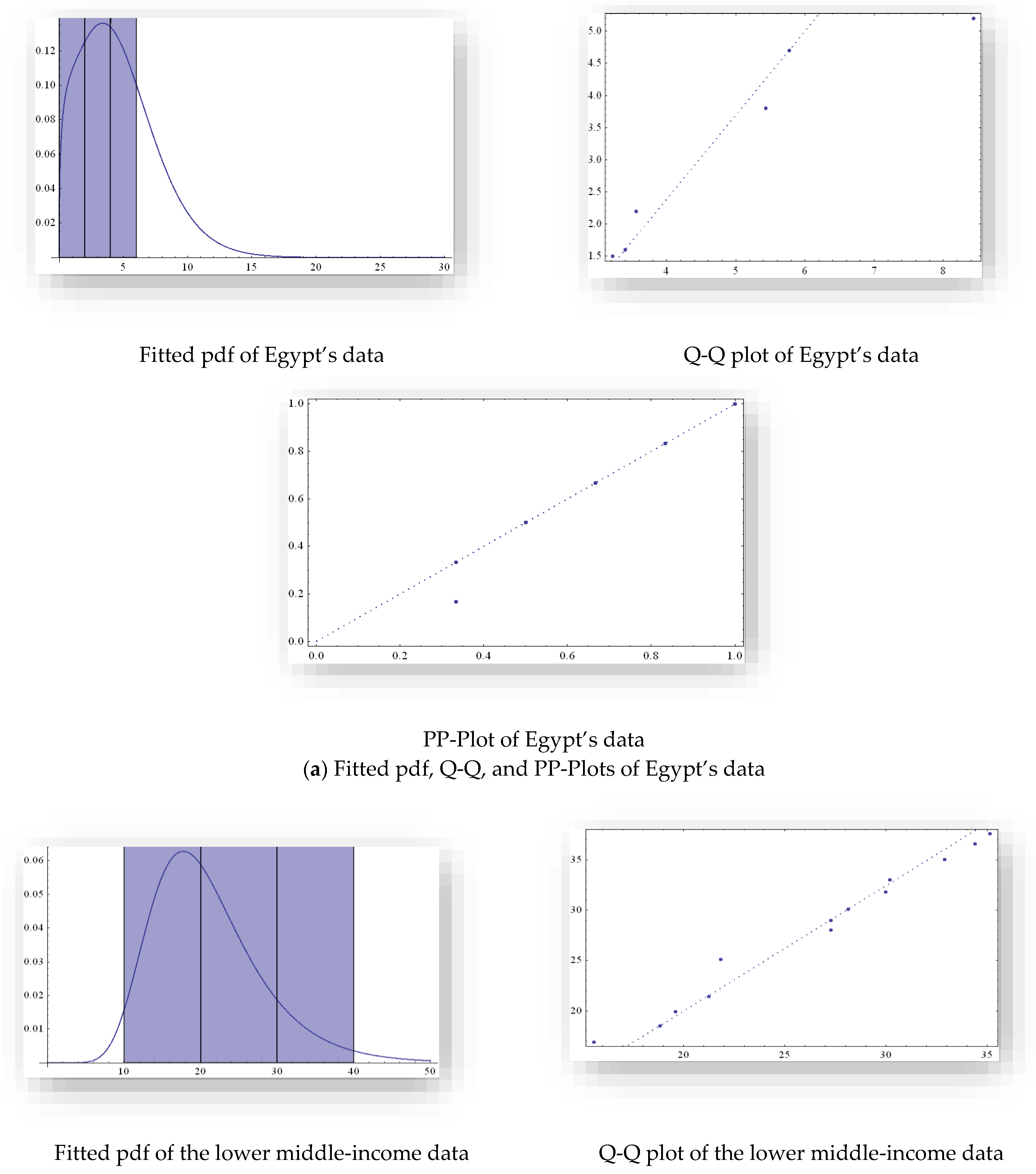
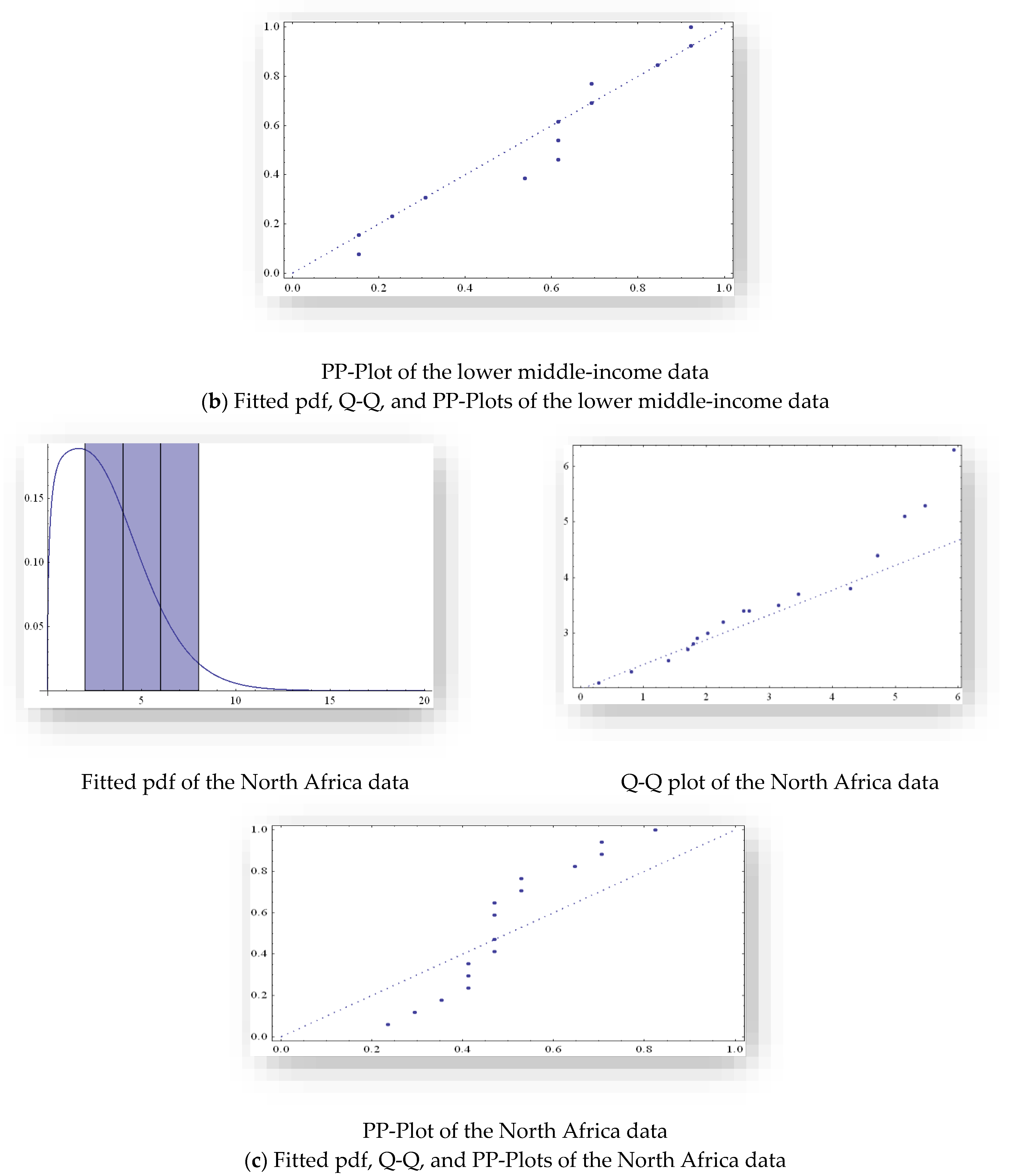
To check the validity of the fitted model, the Kolmogorov–Smirnov goodness of fit test is performed for each dataset, and the p values in each case indicate that the model fits the data very well. Figure 4 displays the fitted pdf, PP-Plot, and Q-Q plot of the EG-Xg distribution for the vinyl chloride data. Also, Figure 5 and Figure 6 show the fitted pdf, PP-Plot, and Q-Q plot of the EG-Xg distribution for the poverty headcount ratio data. 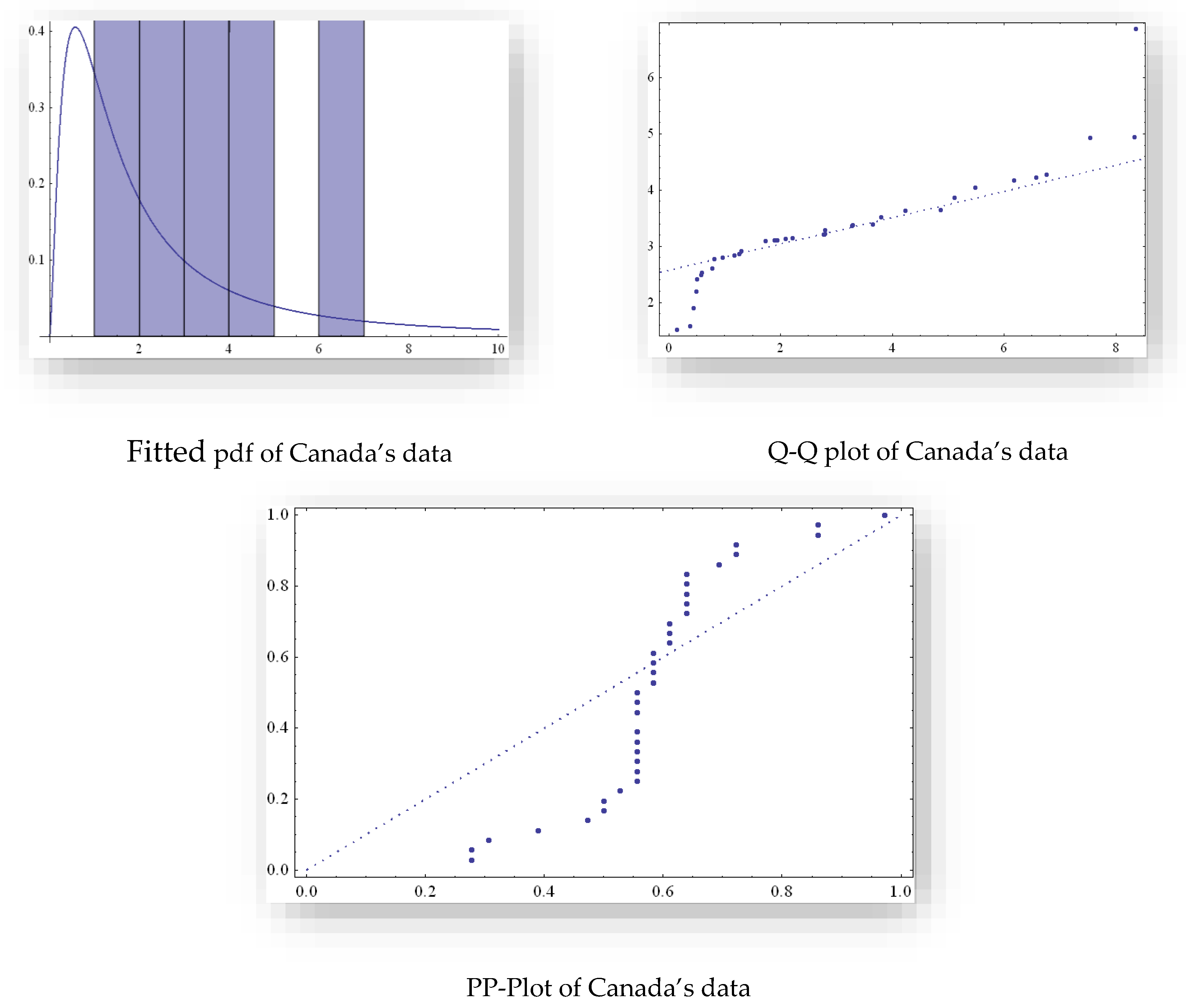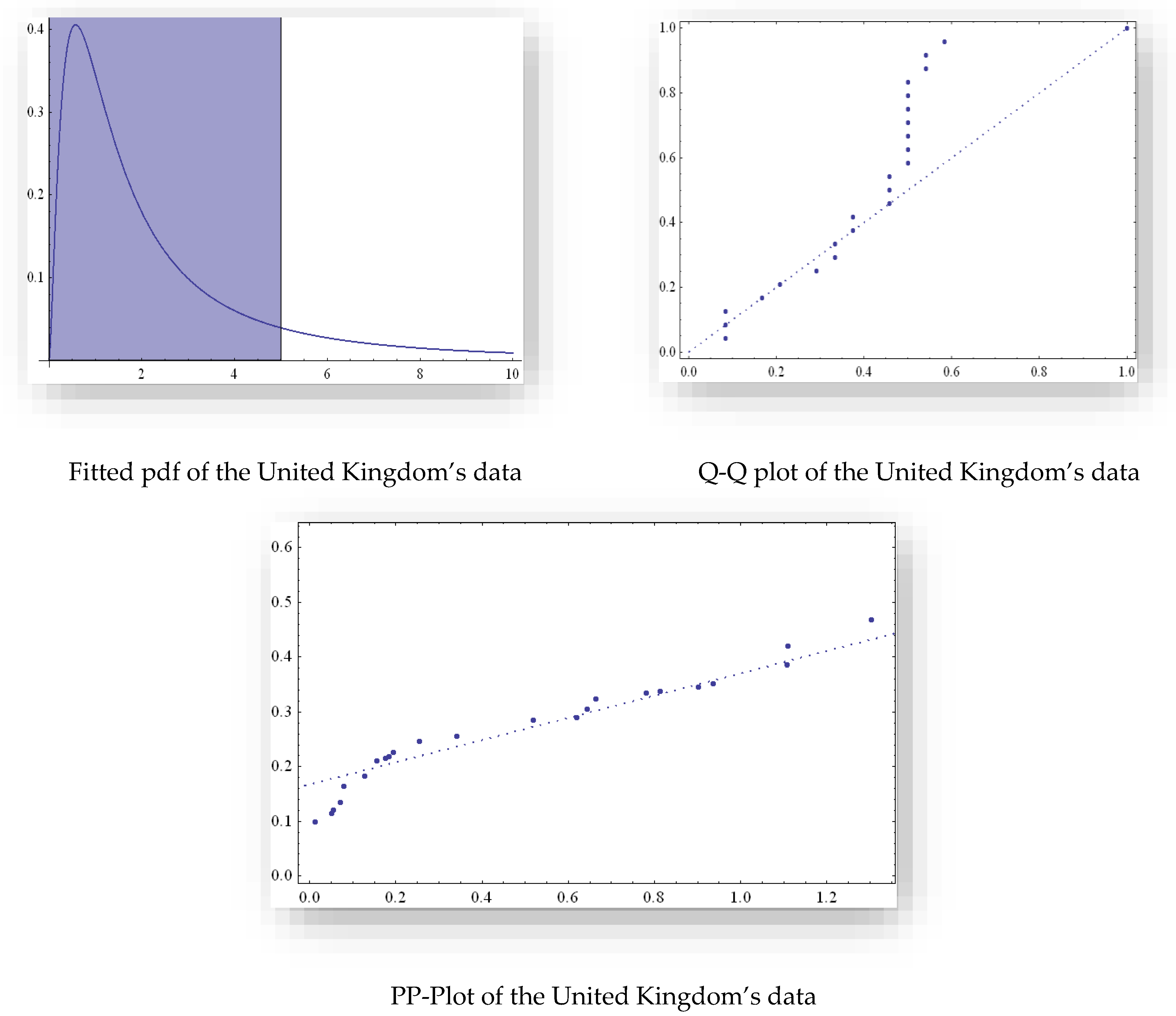Figure 7 and Figure 8 exhibit the fitted pdf, Q-Q plot, and PP-Plot of the EG-Xg distribution for the two real datasets of COVID-19, which indicate that the EG-Xg distribution provides better fits to these data.

I.

The data of the first application is the vinyl chloride data obtained from clean upgradient groundwater monitoring wells in mg/L; this dataset was used by [35]. The data are: 5.1, 1.2, 1.3, 0.6, 0.5, 2.4, 0.5, 1.1, 8.0, 0.8, 0.4, 0.6, 0.9, 0.4, 2.0, 0.5, 5.3, 3.2, 2.7, 2.9, 2.5, 2.3, 1.0, 0.2, 0.1, 0.1, 1.8, 0.9, 2.0, 4.0, 6.8, 1.2, 0.4, and 0.2.

From the data, one can observe that the following are lower record values: 5.1, 1.2, 0.6, 0.5, 0.4, 0.2, and 0.1, with p-value = 0.566.

II.

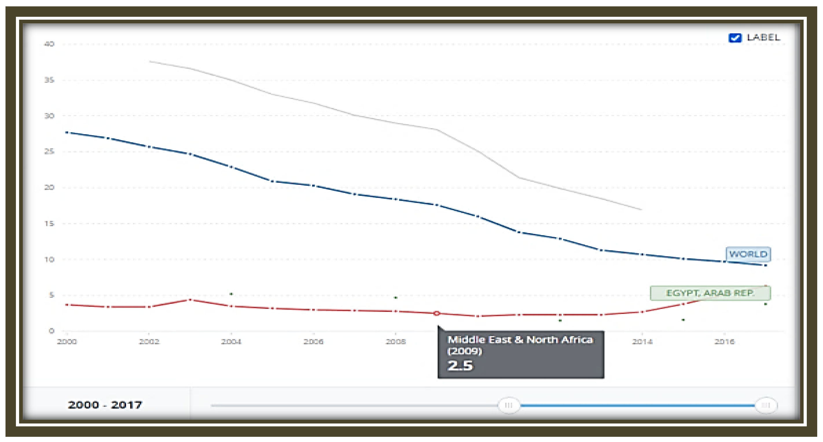
The second application is for economic data, which are the poverty headcount ratio at USD 1.90 a day (2011 purchasing power parity) (% of population) from https://data.worldbank.org/topic/poverty (accessed on 10 June 2021)

(a)

Egypt’s data (2000–2017) are as follows: 5.2, 4.7, 2.2, 1.5, 1.6, and 3.8.

From the data, one can observe that the following are lower record values: 5.2, 4.7, 2.2, and 1.5, with p-value = 0.55

(b)

The lower middle-income data (2000–2017) are as follows: 37.6, 36.6, 35, 33, 31.8, 30.1, 29, 28, 25.1, 21.4, 19.9, 18.5, and 16.9.

From the data, one can observe that the following are lower record values: 37.6, 36.6, 35, 33, 31.8, 30.1, 29, 28, 25.1, 21.4, 19.9, 18.5, and 16.9, with p-value = 0.126

(c)

The Middle Eastern and North African data (2000–2017) are: 3.7, 3.4, 3.4, 3.4, 3.4, 3.2, 3, 2.9, 2.8, 2.5, 2.1, 2.3, 2.3, 2.3, 2.7, 3.8, 5.1, and 6.3.

From the data, one can observe that the following are lower record values: 3.7, 3.4, 3.2, 3, 2.9, 2.8, 2.5, and 2.1, with p-value = 0.358.

III.

Application of COVID-19 data

1.

The first data for this application represent a COVID-19 dataset from Canada covering 36 days, from 10 April to 15 May 2020 (see [36]). These data are mortality rates, used by [37]. The data are as follows: 3.1091, 3.3825, 3.1444, 3.2135, 2.4946, 3.5146, 4.9274, 3.3769, 6.8686, 3.0914, 4.9378, 3.1091, 3.2823, 3.8594, 4.0480, 4.1685, 3.6426, 3.2110, 2.8636, 3.2218, 2.9078, 3.6346, 2.7957, 4.2781, 4.2202, 1.5157, 2.6029, 3.3592, 2.8349, 3.1348, 2.5261, 1.5806, 2.7704, 2.1901, 2.4141, and 1.9048.

From the data, one can observe that the lower record values are: 3.1091, 2.4946, 1.5157, with p-value = 0.124

2.

The second dataset represents COVID-19 data which is from the United Kingdom over a period of 24 days, from 15 October to 7 November 2020 [36]. These data are mortality rates and were used by [37]. The data are as follows: 0.2240, 0.2189, 0.2105, 0.2266, 0.0987, 0.1147, 0.3353, 0.2563, 0.2466, 0.2847, 0.2150, 0.1821, 0.1200, 0.4206, 0.3456, 0.3045, 0.2903, 0.3377, 0.1639, 0.1350, 0.3866, 0.4678, 0.3515, and 0.3232.

From the data, one can notice that the lower record values are: 0.2240, 0.2189, 0.2105, 0.0987, with p-value = $0.12$.

Remark 1. 

The results presented in this paper can be extended to obtain specific results for sub-models of the EG-Xg distribution, as follows:

• The exponentiated Xg distribution, if $\alpha =1$.
• The Xg distribution, if $\alpha =1 and \beta =1$.

4.3. Concluding Remarks

○

It is noticed from Table 1 and Table 2 that the ML averages become very close to the population parameter values as the sample size increases. Also, ERs decrease when the sample size increases. This reflects that the estimates become more accurate, consistent, and approach the population parameter values as the sample size increases.

○

It is noticed that the ERs of the rf and hrf decrease when the sample size increases. This indicates that as the sample size increases, the accuracy of the estimated values for the rf and hrf improves, i.e., the difference between the estimated values and the true values decreases as the sample size becomes larger. In other words, as the sample size increases, the estimates become more precise and reliable. This is because with a larger sample, we have more information about the underlying population, which leads to more accurate estimates. Also, it suggests that the proposed estimation methods (ML and Bayesian) are consistent and efficient and that as the sample size increases, the estimates converge to the true population parameters, and the estimates become more reliable.

○

The lengths of the CIs of the parameters, rf, and hrf become narrower as the sample size increases. This indicates that the estimates are more precise, which can lead to better decision-making, especially in certain fields, like reliability engineering and survival analysis. Also, when the length becomes narrower, we become more confident in the accuracy of our estimates for the rf and hrf. This is because larger sample sizes provide more information about the underlying population, leading to more precise estimates. Moreover, accurate estimates of the rf and hrf can improve the accuracy of prediction about future events.

○

It is clear from Table 3 and Table 4 that the ERs of the Bayes averages of the parameters perform better, which reflects that the Bayes estimates become closer to the true parameter values. The length of the credible intervals becomes shorter when the sample size of Rv increases, which indicates higher precision of the estimates. This suggests that Bayesian estimation is a robust and effective method for estimating the parameters, particularly when dealing with smaller sample sizes.

○

From Table 5, one can notice that the ERs of the rf and hrf perform better when the sample size of Rv increases, which indicates that the estimated values for the rf and hrf become more accurate. The lengths of the credible intervals become shorter when the sample size of Rv increases; this means that the true values of these parameters are likely to be closer to the estimated values and that larger sample sizes lead to more accurate and reliable results.

○

One can notice that the ERs for the averages of the parameters, rf, and hrf under the LINEX loss function have lower values than the corresponding ERs of the averages under the SE loss function. This reflects the fact that the LINEX loss function provides more robust and accurate estimates for the parameters of interest compared to the SE loss function.

○

It is clear from Table 9, Table 10 and Table 11 that the standard errors for the estimates of the parameters, rf, and hrf under the LINEX loss function have lower values than the corresponding ERs of the estimates under the SE loss function. This means that the estimates are more concentrated around the true parameter values, reducing the uncertainty associated with the estimates. Also, it indicates that the LINEX loss function provides more accurate and precise estimates for the parameters of interest.

Future research directions include investigating alternative estimation methods, such as modified maximum likelihood and modified moment methods. Additionally, exploring the predictive performance of ML and modified ML methods for the EG-Xg distribution under different censoring schemes, such as reversed ordered order statistics and lower Pfeifer records, could be a valuable contribution to the field. Bayesian estimation can be derived considering different types of loss functions (symmetric or asymmetric), such as balanced loss functions, for example balanced absolute, balanced binary, balanced modified LINEX, and balanced general entropy loss functions. Also, prediction (point and interval) for future observation can be obtained using different loss functions under different censoring schemes. Recurrence relations for single and product moments based on the dgos of the EG-Xg distribution can be studied [See [38,39,40]].