Theoretical Aspects for Bayesian Predictions Based on Three-Parameter Burr-XII Distribution and Its Applications in Climatic Data

Abstract

Symmetry and asymmetry play vital roles in prediction. Symmetrical data, which follows a predictable pattern, is easier to predict compared to asymmetrical data, which lacks a predictable pattern. Symmetry helps identify patterns within data that can be utilized in predictive models, while asymmetry aids in identifying outliers or anomalies that should be considered in the predictive model. Among the various factors associated with storms and their impact on surface temperatures, wind speed stands out as a significant factor. This paper focuses on predicting wind speed by utilizing unified hybrid censoring data from the three-parameter Burr-XII distribution. Bayesian prediction bounds for future observations are obtained using both one-sample and two-sample prediction techniques. As explicit expressions for Bayesian predictions of one and two samples are unavailable, we propose the use of the Gibbs sampling process in the Markov chain Monte Carlo framework to obtain estimated predictive distributions. Furthermore, we present a climatic data application to demonstrate the developed uncertainty procedures. Additionally, a simulation research is carried out to examine and contrast the effectiveness of the suggested methods. The results reveal that the Bayes estimates for the parameters outperformed the Maximum likelihood estimators.

1. Introduction

Wind is the force that converts air pressure into air movement, causing the speed of the wind to decrease as air pressure increases. When a mass of moving air slows down, its kinetic energy or momentum is converted into static atmospheric pressure. This relationship indicates that higher wind speeds correspond to lower air pressure measurements. In addition to transporting hot or cold air, wind introduces moisture into the atmosphere, resulting in changes in weather patterns. Therefore, changes in wind conditions directly impact the weather. The direction of the wind is influenced by differences in air pressure. Wind flows from areas of high pressure to low-pressure zones, and the wind’s speed determines the degree of cooling. The UHCS, a generalised Type-I and Type-II HCS, was first introduced by Balakrishnan et al. [1]. The following is a definition of it: Let $T_1$ and $T_2$ be values within the range $(0,\infty )$, where $T_2$ is greater than $T_1$, and let r and K be integers such that $K<r<n$. The test ends at min{max {$Z_{r:n},T_1\},T_2$} if the Kth failure occurs before time $T_1$, where $Z_{r:n}$ represents the failure time of the rth unit. The test ends at the earliest possible time between $Z_{r:n}$ and $T_2$ if the Kth failure occurs between $T_1$ and $T_2$. If the kth failure occurs after time $T_2$, the experiment is terminated at $Z_{K:n}$, where $Z_{K:n}$ denotes the failure time of the Kth unit. By employing this censoring scheme, we can ensure that the experiment concludes within a maximum duration of $T_2$ with at least K failures. In such case, we can assure exactly K failures. The Burr-XII distribution was first developed by Burr [2] and has been effectively used with a wide variety of observational data in many different fields. See Shao [3], Wu et al. [4] and Silva et al. [5] for more information on Burr-XII’s applications. There are several reasons for choosing the Burr distribution. Firstly, it encompasses only positive values, making it particularly suitable for modeling hydrological or meteorological data. Secondly, it possesses two shape parameters, enabling its adaptability to different samples due to its ability to cover a wide range of skewness and kurtosis values. For further discussion on this aspect, see Ganora and Laio [6]. Thirdly, the Burr-XII family is extensive and includes various sub-models, such as the log-logistic distribution. Cook and Johnson [7] utilized the Burr model to achieve improved fits for a uranium survey dataset, while Zimmer et al. [8] explore the statistical and probabilistic properties of the Burr-XII distribution and its relationship with other distributions commonly used in reliability analysis. Tadikamalla [9] expanded the two-parameter Burr-XII distribution by introducing an additional scale parameter, resulting in the TPBXIID. Since then, the applications of the Burr-XII distribution have received increased attention. Tadikamalla also established mathematical relationships among Burr-related distributions, demonstrating that the Lomax distribution is a special case of the Burr-XII distribution, and the compound Weibull distribution generalizes the Burr distribution. Furthermore, Tadikamalla showed that the Weibull, logistic, log-logistic, normal, and lognormal distributions can be considered as special cases of the Burr-XII distribution through appropriate parameter choices. The TPBXIID offers significant flexibility by incorporating two shape parameters and one scale parameter into its distribution function, allowing for a wide range of distribution shapes. The TPBXIID is defined by the following cdf:

$$F(z;\alpha ,\theta ,\gamma )=1-{\left[1+{\left(\frac{z}{\alpha }\right)}^{\theta }\right]}^{-\gamma },z>0,\alpha ,\theta ,\gamma >0,$$

(1)

and the pdf is given by:

$$f(z;\alpha ,\theta ,\gamma )=\theta \gamma {\alpha }^{-\theta }{z}^{\theta -1}{\left[1+{\left(\frac{z}{\alpha }\right)}^{\theta }\right]}^{-(\gamma +1)},z>0,\alpha ,\theta ,\gamma >0,$$

(2)

The survival function $S\left(z\right)$ can be obtained as:

$$S\left(z\right)={\left[1+{\left(\frac{z}{\alpha }\right)}^{\theta }\right]}^{-\gamma },z>0,$$

(3)

and the failure rate function $h\left(z\right)$ is given by:

$$h\left(z\right)=\theta \gamma {\alpha }^{-\theta }{z}^{\theta -1}{\left[1+{\left(\frac{z}{\alpha }\right)}^{\theta }\right]}^{-1},z>0,$$

(4)

where the parameters $\gamma$ and $\theta$ determine the shape of the density function, while $\alpha$ determines its scale. When $\theta$ is greater than 1, the function has a shape that resembles an upside-down bathtub and is unimodal, with the mode occurring at $z=\alpha {\left[\frac{(\theta -1)}{(\theta \gamma +1)}\right]}^{\frac{1}{\theta }}$. In the case where $\theta$ is equal to 1, the function has an L-shape.

The TPBXIID can be reduced to well-known distributions as follows:

• Setting $\theta =1$ in Equation (1) results in the Lomax distribution.
• Setting $\alpha =1$ in Equation (1) leads to the Burr-XII distribution.
• Setting $\alpha =1$ and $\gamma =1$ in Equation (1) yields the log-logistic distribution.

The shapes of the pdf, cdf, survival and failure rate functions of the TPBXIID for different values of the parameters $\alpha$, $\theta$ and $\gamma$ are given in the Figure 1, Figure 2, Figure 3 and Figure 4.

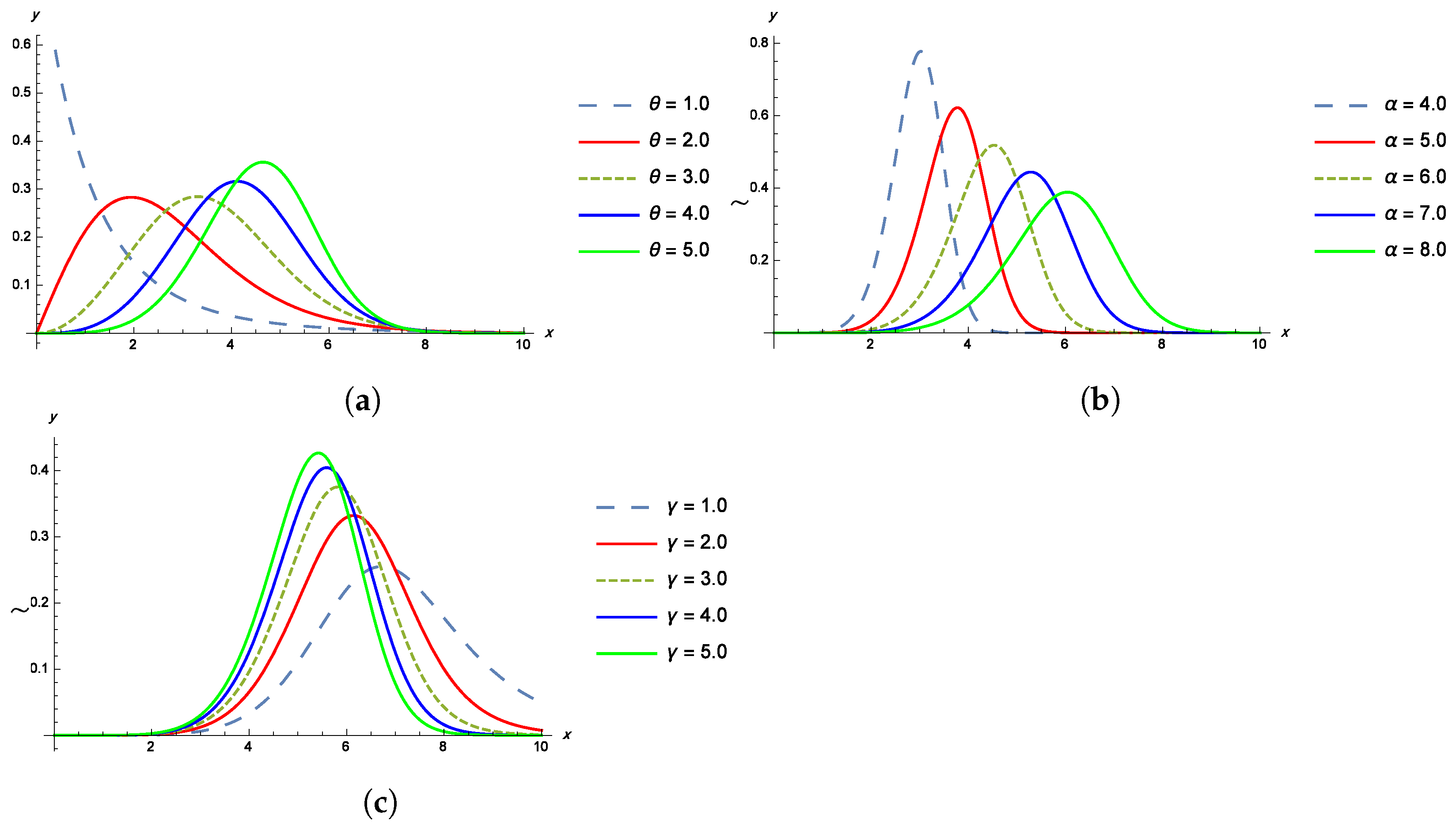
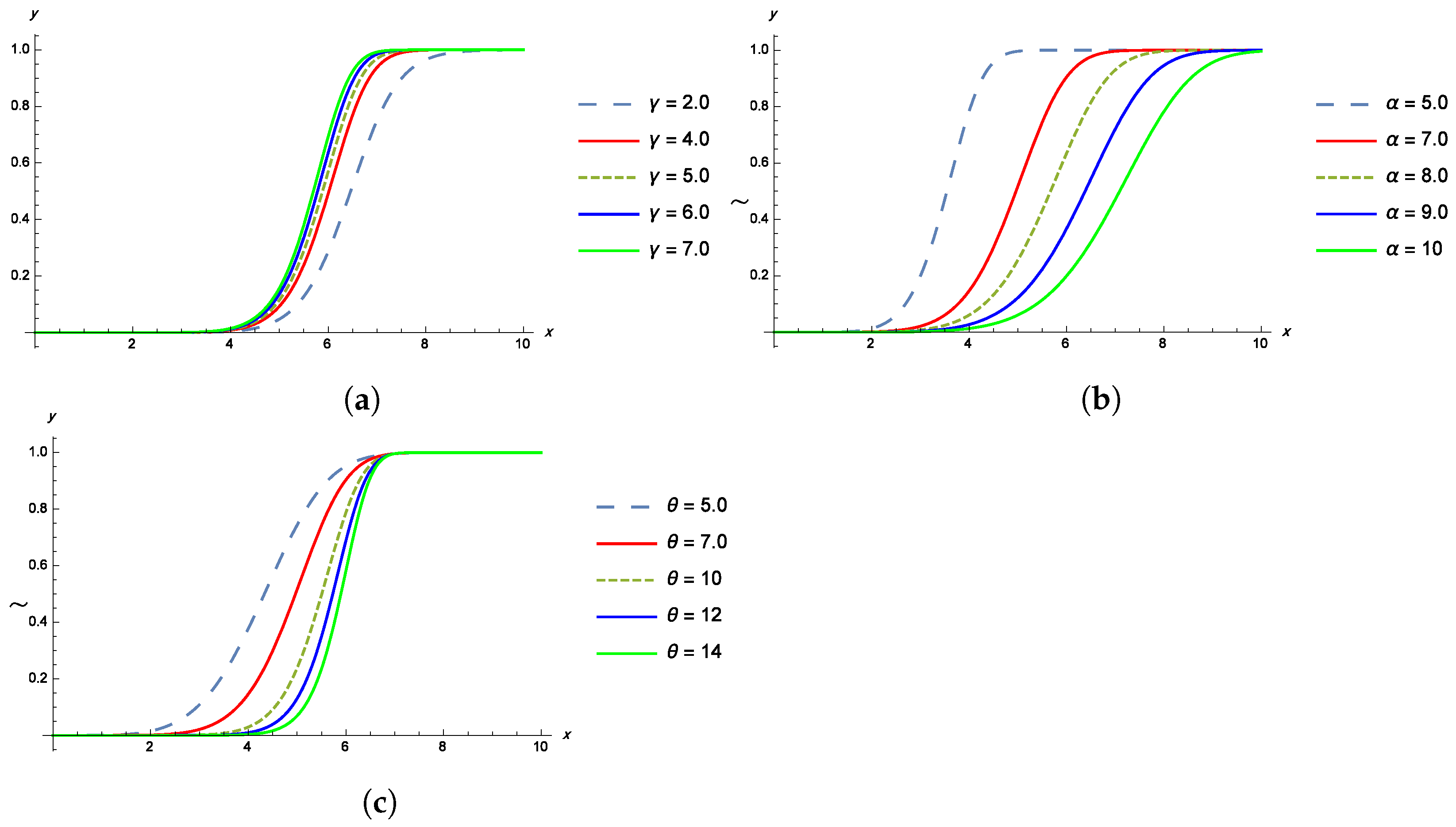
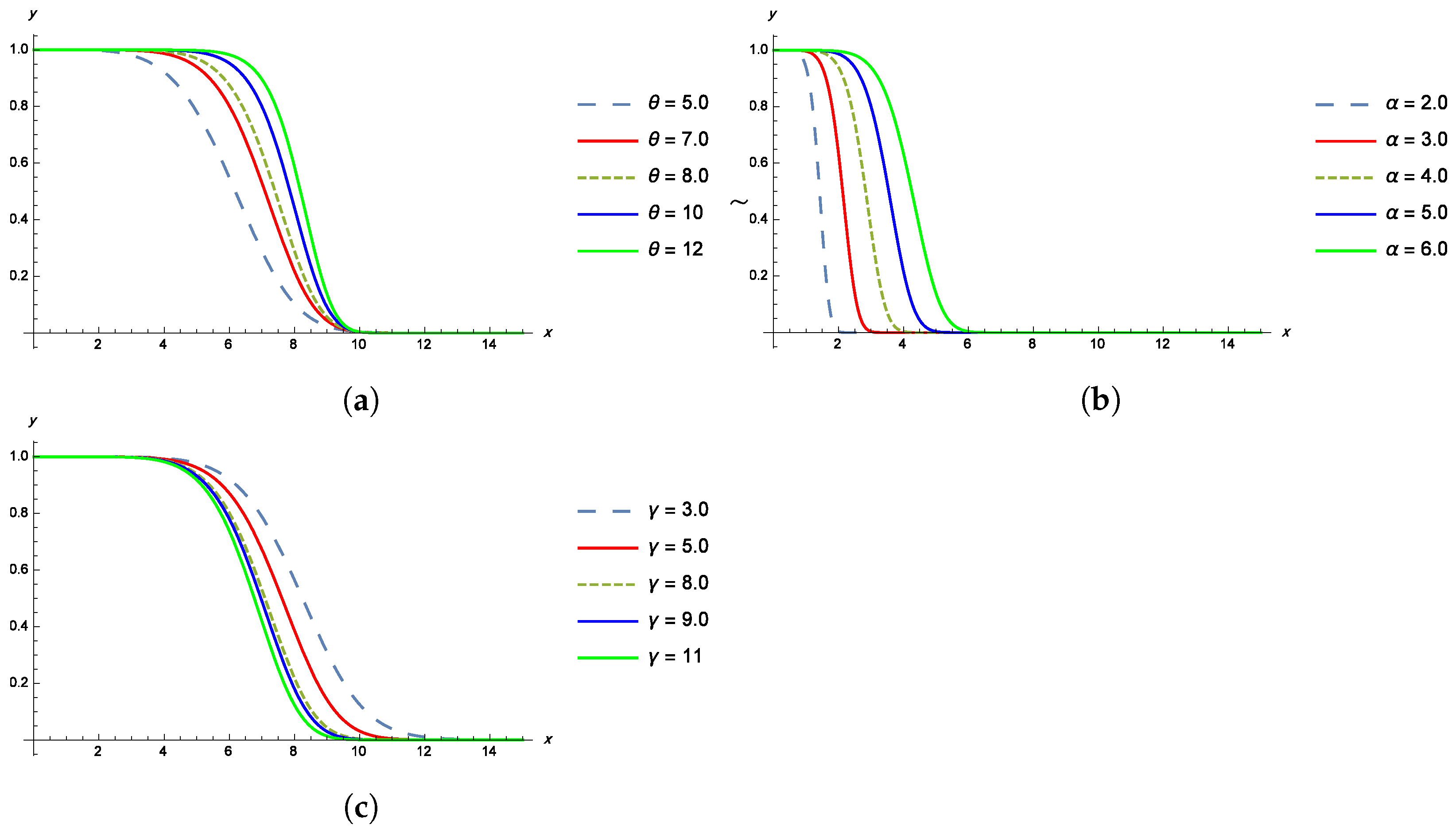
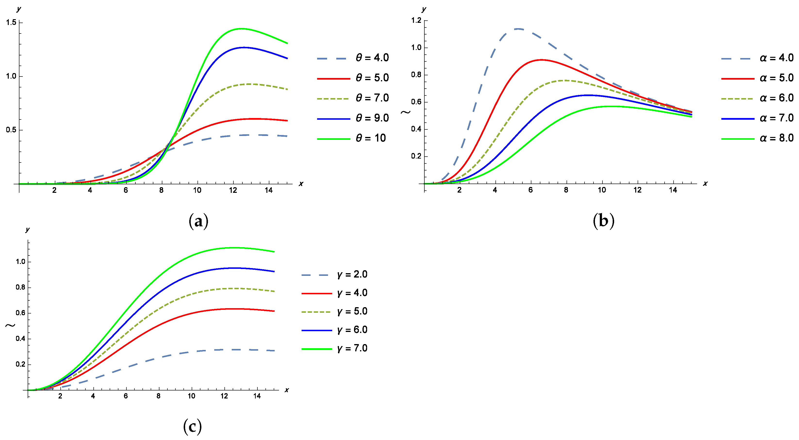
Properties of the TPBXIID

• The rth moment about the origin of a random variable Z distributed by a TPBXIID, denoted by $\acute{{\mu }_r}$, is the expected value of $Z^r$, symbolically,

  $$\begin{array}{c}\hfill \acute{{\mu }_r}=E\left(Z^r\right)=\frac{{\alpha }^r\Gamma (\frac{r}{\theta }+1)\Gamma (\gamma -\frac{r}{\theta })}{\Gamma \left(\gamma \right)},\end{array}$$

  (5)

  where

  $$\Gamma (\gamma -\frac{r}{\theta })\ne 0,-1,-2,\dots ,-\infty .$$
• The variance of TPBXIID can be written as

  $$\begin{array}{c}\hfill {\theta }^2=\frac{{\alpha }^2\Gamma \left(\gamma \right)\Gamma (\frac{2}{\theta }+1)\Gamma (\gamma -\frac{2}{\theta })-{\alpha }^2\Gamma {(\frac{1}{\theta }+1)}^2\Gamma {(\gamma -\frac{1}{\theta })}^2}{\Gamma {\left(\gamma \right)}^2}.\end{array}$$

  (6)
• The $q^{th}$ quantile $z_q$ of the TPBXIID can be defined as

  $$z_q=\alpha {\left[{\left(1-q\right)}^{\frac{-1}{\gamma }}-1\right]}^{\frac{1}{\theta }}.$$

  (7)

Belaghi and Asl conducted research on estimating the Burr-XII distribution using both non-Bayesian and Bayesian methods in recent studies [10]. Another study by Nasir et al. [11] introduced a new category of distributions, called Burr-XII power series, which has a strong physical basis and combines the exponentiated Burr-XII and power series distributions. Additionally, Jamal et al. [12] proposed an altered version of the TPBXIID distribution that has flexible hazard rate shapes based on the common Burr-XII distribution.This study has been examined by multiple authors, including Sen et al. [13], Dutta and Kayal [14], Dutta et al. [15], and Sagrillo et al. [16].

Prediction plays a significant role in inferential statistics and is of great importance in various practical domains such as meteorology, economics, engineering, and education greatly rely on prediction for making informed decisions. Many life-testing experiments involve predicting future observations. Several researchers, including Balakrishnan and Shafay [17], AL-Hussaini and Ahmad [18], Shafay and Balakrishnan [19] and Shafay [20,21] have explored Bayesian prediction methods for future observations using various types of observed data.

Recently, Ateya et al. [22] conducted a study on predicting future failure times using a UHCS for the Burr-X model, with specific emphasis on engineering applications. In this article, we address the same problem using UHCS but with additional considerations. Let $Z_{1:n}<Z_{2:n}<\dots <Z_{n:n}$ denote the order statistics from a random sample of size n from an absolutely continuous distribution. Under the UHCS, we run into six situations, which are listed below:

(I)

$0<z_{k:n}<z_{r:n}<T_1<T_2$,

(II)

$0<z_{k:n}<T_1<z_{r:n}<T_2$,

(III)

$0<z_{k:n}<T_1<T_2<z_{r:n}$,

(IV)

$0<T_1<z_{k:n}<z_{r:n}<T_2$,

(V)

$0<T_1<z_{k:n}<T_2<z_{r:n}$,

(VI)

$0<T_1<T_2<z_{k:n}<z_{r:n}$.

In each situation, the experiment is terminated at $T_1$, $z_{r:n}$, $T_2$, $z_{r:n}$, $T_2$, and $z_{k:n}$, respectively. Thus, the likelihood function of the UHCS $\underline{Z}=(Z_{1:n}<Z_{2:n}<\dots <Z_{W:n})$ can be expressed as:

$$L(\underline{z},\theta )=\frac{n!}{(n-W)!}\left[\prod _{i=1}^{W}f\left(z_i\right)\right]{\left[1-F\left(B\right)\right]}^{n-W},$$

(8)

$$(W,B)=\left\{\begin{array}{cc}(G_1,T_1),\hfill & \mathrm{for}\mathrm{I},\hfill \\ (r,z_{r:n}),\hfill & \mathrm{for}\mathrm{II}\mathrm{and}\mathrm{IV},\hfill \\ (G_2,T_2),\hfill & \mathrm{for}\mathrm{III}\mathrm{and}\mathrm{V},\hfill \\ (k,z_{k:n}),\hfill & \mathrm{for}\mathrm{VI},\hfill \end{array}\right.$$

(9)

In this context, W represents the cumulative number of failures observed in the experiment up to time B (the stopping time point), and $G_1$ and $G_2$ indicate the number of failures that have occurred before time points $T_1$ and $T_2$, respectively.

Moreover, using Equations (1), (2) and (8), we can express the likelihood function as:

$$L(\underline{z};\alpha ,\theta ,\gamma )=K{\alpha }^{-W\theta }{\theta }^W{\gamma }^W\prod _{i=1}^W{z}_i^{\theta -1}\prod _{i=1}^W{\left[1+{\left(\frac{z_i}{\alpha }\right)}^{\theta }\right]}^{-(\gamma +1)}{\left[1+{\left(\frac{B}{\alpha }\right)}^{\theta }\right]}^{-\gamma (n-W)},$$

(10)

where $K=\frac{n!}{(n-W)!}$.

The log-likelihood function for Equation (10), can be expressed as follows:

$$\begin{array}{cc}\hfill \mathcal{l}(\alpha ,\theta ,\gamma )=& ln\left(k\right)+Wln\theta -W\theta ln\alpha +Wln\gamma +(\theta -1)\sum _{i=1}^{W}ln\left(z_i\right)-(\gamma +1)\sum _{i=1}^{W}ln\left[1+{\left(\frac{z_i}{\alpha }\right)}^{\theta }\right]\hfill \\ & -\gamma (n-W)ln\left[1+{\left(\frac{B}{\alpha }\right)}^{\theta }\right].\hfill \end{array}$$

(11)

To obtain the parameter estimates, we calculate the first derivatives of Equation (11) as follows:

$$\frac{-W\widehat{\theta }}{\widehat{\alpha }}+(\widehat{\gamma }+1)\sum _{i=1}^W\frac{\widehat{\theta }{z}_i{\left(\frac{z_i}{\widehat{\alpha }}\right)}^{\widehat{\theta }-1}}{{\alpha }^2\left[1+{\left(\frac{z_i}{\widehat{\alpha }}\right)}^{\widehat{\theta }}\right]}+\widehat{\gamma }(n-W)\frac{\widehat{\theta }B{\left(\frac{B}{\widehat{\alpha }}\right)}^{\widehat{\theta }-1}}{{\alpha }^2\left[1+{\left(\frac{B}{\widehat{\alpha }}\right)}^{\widehat{\theta }}\right]}=0,$$

(12)

$$\frac{W}{\widehat{\theta }}-Wln\widehat{\alpha }+\sum _{i=1}^{W}ln{z}_i-(\widehat{\gamma }+1)\sum _{i=1}^W\frac{{\left(\frac{z_i}{\widehat{\alpha }}\right)}^{\widehat{\theta }}ln\left(\frac{z_i}{\widehat{\alpha }}\right)}{1+{\left(\frac{z_i}{\widehat{\alpha }}\right)}^{\widehat{\theta }}}-\widehat{\gamma }(n-W)\frac{{\left(\frac{B}{\widehat{\alpha }}\right)}^{\widehat{\theta }}ln\left(\frac{B}{\widehat{\alpha }}\right)}{1+{\left(\frac{B}{\widehat{\alpha }}\right)}^{\widehat{\theta }}}=0,$$

(13)

and

$$\frac{W}{\widehat{\gamma }}-\sum _{i=1}^{W}ln\left[1+{\left(\frac{z_i}{\widehat{\alpha }}\right)}^{\widehat{\theta }}\right]-(n-W)ln\left[1+{\left(\frac{B}{\widehat{\alpha }}\right)}^{\widehat{\theta }}\right]=0.$$

(14)

From (14), we obtain the MLE $\widehat{\gamma }$ as

$$\widehat{\gamma }=W{\left[\sum _{i=1}^{W}ln\left[1+{\left(\frac{z_i}{\widehat{\alpha }}\right)}^{\widehat{\theta }}\right]+(n-W)ln\left[1+{\left(\frac{B}{\widehat{\alpha }}\right)}^{\widehat{\theta }}\right]\right]}^{-1}.$$

(15)

Because Equations (12) and (13) cannot be written in closed-form expressions, we propose that the parameters have gamma prior distributions as follows:

$${\pi }_1\left(\alpha \right)\propto {\alpha }^{a_1-1}{e}^{-b_1\alpha },\alpha >0,$$

$${\pi }_2\left(\theta \right)\propto {\theta }^{a_2-1}{e}^{-b_2\theta },\theta >0,$$

$${\pi }_3\left(\gamma \right)\propto {\gamma }^{a_3-1}{e}^{-b_3\gamma },\gamma >0,$$

The expression

$$\pi (\alpha ,\theta ,\gamma )\propto {\alpha }^{a_1-1}{\theta }^{a_2-1}{\gamma }^{a_3-1}{e}^{-b_1\alpha -b_2\theta -b_3\gamma },$$

(16)

represents the joint prior distribution for the $\alpha$, $\theta$ and $\gamma$ The joint posterior density function is obtained from (8) and (16) as follows:

$$\begin{array}{cc}\hfill {\pi }^{*}(\alpha ,\theta ,\gamma |\underline{z})\propto & {\alpha }^{a_1-W\theta -1}{\theta }^{a_2+W-1}{\gamma }^{a_3+W-1}{e}^{-\theta \left\{b_2-{\sum }_{i=1}^{W}ln\left(z_i\right)\right\}}{e}^{-\gamma \left\{b_3+{\sum }_{i=1}^{W}ln\left[1+{\left(\frac{z_i}{\alpha }\right)}^{\theta }\right]\right\}}\hfill \\ & \times e^{-b_1\alpha -{\sum }_{i=1}^{W}ln\left[1+{\left(\frac{z_i}{\alpha }\right)}^{\theta }\right]}{\left[1+{\left(\frac{B}{\alpha }\right)}^{\theta }\right]}^{-\gamma (n-W)}.\hfill \end{array}$$

(17)

The posterior density function of $\alpha$ given $\theta$ and $\gamma$ can be derived from (17) and is expressed as:

$${\pi }_1^{*}\left(\alpha \right|\theta ,\gamma ,\underline{z})\propto {\alpha }^{a_1-W\theta -1}{e}^{-b_1\alpha -{\sum }_{i=1}^{W}ln\left[1+{\left(\frac{z_i}{\alpha }\right)}^{\theta }\right]}{\left[1+{\left(\frac{B}{\alpha }\right)}^{\theta }\right]}^{-\gamma (n-W)},$$

(18)

$${\pi }_2^{*}\left(\theta \right|\alpha ,\gamma ,\underline{z})\propto {\theta }^{a_2+W-1}{\alpha }^{a_1-W\theta -1}{e}^{-\theta \left\{b_2-{\sum }_{i=1}^{W}ln\left(z_i\right)\right\}}{e}^{-{\sum }_{i=1}^{W}ln\left[1+{\left(\frac{z_i}{\alpha }\right)}^{\theta }\right]},$$

(19)

and

$${\pi }_3^{*}\left(\gamma \right|\alpha ,\theta ,\underline{z})\propto {\gamma }^{a_3+W-1}{e}^{-\gamma \left\{b_3+{\sum }_{i=1}^{W}ln\left[1+{\left(\frac{z_i}{\alpha }\right)}^{\theta }\right]\right\}}.$$

(20)

It can be seen that, generating samples of $\gamma$ can be achieved easily using any routine that produces random numbers from a gamma distribution. However, the posterior density functions of $\alpha$ given $\theta$ and $\gamma$ in (18), and the posterior density function of $\theta$ given $\alpha$ and $\gamma$ in (19), do not have known distributions that allow for direct sampling using conventional techniques. Despite this, when observing the plots of both posterior distributions, it becomes apparent that they exhibit similarities to normal distributions, as depicted in Figure 5. Therefore, we recommend employing the Metropolis–Hastings algorithm with a normal proposal distribution to generate random numbers from these distributions, as suggested by Metropolis et al. [23]. The subsequent sections of this paper are organized as follows: Section 2 examines Bayesian prediction intervals utilizing the UHCS for the TPBXIID. In Section 3, we employ the MCMC technique to derive Bayesian prediction intervals. Section 4 presents an analysis of a real dataset for illustrative purposes. Finally, Section 5 offers concluding remarks.

2. Approximate Confidence Interval

The asymptotic variance–covariance of the MLEs for the parameters $\alpha$, $\theta$, and $\gamma$ can be determined by the elements of the negative Fisher information matrix, denoted as $I_{ij}$. These elements are defined as follows:

$$I_{ij}=-E\left(\begin{array}{c}\frac{{\partial }^2\mathcal{l}}{\partial {\chi }_i\partial {\chi }_j}\end{array}\right);\mathrm{where}i,j=1,2,3\mathrm{and}({\chi }_1,{\chi }_2,{\chi }_3)=(\alpha ,\theta ,\gamma ).$$

(21)

Finding exact mathematical formulas for these assumptions is difficult, though. The variance-covariance matrix is therefore calculated as follows:

$$I^{-1}(\alpha ,\theta ,\gamma )={\left(\begin{array}{ccc}-\frac{{\partial }^2\mathcal{l}}{\partial {\alpha }^2}& -\frac{{\partial }^2\mathcal{l}}{\partial \alpha \partial \theta }& -\frac{{\partial }^2\mathcal{l}}{\partial \alpha \partial \gamma }\\ -\frac{{\partial }^2\mathcal{l}}{\partial \theta \partial \alpha }& -\frac{{\partial }^2\mathcal{l}}{\partial {\theta }^2}& -\frac{{\partial }^2\mathcal{l}}{\partial \theta \partial \gamma }\\ -\frac{{\partial }^2\mathcal{l}}{\partial \gamma \partial \alpha }& -\frac{{\partial }^2\mathcal{l}}{\partial \gamma \partial \theta }& -\frac{{\partial }^2\mathcal{l}}{\partial {\gamma }^2}\end{array}\right)}_{\downarrow (\alpha ,\theta ,\gamma )=(\widehat{\alpha },\widehat{\theta },\widehat{\gamma })}^{-1}=\left(\begin{array}{ccc}\widehat{var}\left(\widehat{\alpha }\right)& cov(\widehat{\alpha },\widehat{\theta })& cov(\widehat{\alpha },\widehat{\gamma })\\ cov(\widehat{\theta },\widehat{\alpha })& \widehat{var}\left(\widehat{\theta }\right)& cov(\widehat{\theta },\widehat{\gamma })\\ cov(\widehat{\gamma },\widehat{\alpha })& cov(\widehat{\gamma },\widehat{\theta })& \widehat{var}\left(\widehat{\gamma }\right)\end{array}\right),$$

(22)

where $\widehat{var}\left(\widehat{\alpha }\right)$, $\widehat{var}\left(\widehat{\theta }\right)$, and $\widehat{var}\left(\widehat{\gamma }\right)$ represent the estimated variances of $\widehat{\alpha }$, $\widehat{\theta }$, and $\widehat{\gamma }$, respectively, while $cov(\widehat{\alpha },\widehat{\theta })$, $cov(\widehat{\alpha },\widehat{\gamma })$, and $cov(\widehat{\theta },\widehat{\gamma })$ denote the estimated covariances between the corresponding parameters. The second derivative is given in Appendix A. Substituting the estimated values $\widehat{\alpha }$, $\widehat{\theta }$, and $\widehat{\gamma }$ into the matrix expression, we obtain the inverse of the asymptotic variance–covariance matrix. Finally, the $(1-\eta )100\%$ confidence intervals for the parameters $\alpha$, $\theta$, and $\gamma$ can be calculated as follows:

$$\begin{array}{c}\hfill \left(\widehat{\alpha }\pm Z_{\eta /2}\sqrt{\widehat{var}\left(\widehat{\alpha }\right)}\right),\left(\widehat{\theta }\pm Z_{\eta /2}\sqrt{\widehat{var}\left(\widehat{\theta }\right)}\right)\mathrm{and}\left(\widehat{\gamma }\pm Z{\gamma }_{\eta /2}\sqrt{\widehat{var}\left(\widehat{\gamma }\right)}\right),\end{array}$$

(23)

where $Z_{\eta /2}$ is the standard normal value.

3. One-Sample Bayesian Prediction

In this section, we introduce a general approach for computing interval predictions for the future order statistic $Z_{c:n}$, which represents the $c^{th}$ observation, within the TPBXIID framework. These predictions are based on the observed UHCS denoted as $\underline{Z}=(Z_{1:n}<Z_{2:n}<\dots <Z_{W:n})$, where $W<c\le n$. For a more comprehensive discussion on Bayesian prediction, please refer to Shafay [20,21]. The conditional density function of $Z_{c:n}$ given the UHCS $\underline{\mathbf{z}}$ can be expressed as follows:

$$f\left(z_s\right|\underline{\mathbf{z}})=\left\{\begin{array}{cc}{f}_1\left(z_c\right|\underline{\mathbf{z}})\mathrm{if}(W,B)=(G_1,T_1),\hfill & \mathrm{for}\mathrm{I},\hfill \\ f_2\left(z_c\right|\underline{\mathbf{z}})\mathrm{if}(W,B)=(r,z_{r:n}),\hfill & \mathrm{for}\mathrm{II}\mathrm{and}\mathrm{IV},\hfill \\ f_3\left(z_c\right|\underline{\mathbf{z}})\mathrm{if}(W,B)=(G_2,T_2),\hfill & \mathrm{for}\mathrm{III}\mathrm{and}\mathrm{for}\mathrm{V},\hfill \\ f_4\left(z_c\right|\underline{\mathbf{z}})\mathrm{if}(W,B)=(k,z_{k:n}),\hfill & \mathrm{for}\mathrm{VI},\hfill \end{array}\right.$$

(24)

where

$$f_1\left(z_c\right|\underline{\mathbf{z}})=\frac{1}{P(r\le G_1\le c-1)}\sum _{g=r}^{c-1}f\left(z_c\right|,\underline{\mathbf{z}},G_1=g)P(G_1=g),$$

$$\begin{array}{cc}\hfill =& \sum _{g=r}^{c-1}\frac{(n-g)!{\varphi }_g\left(T_1\right)}{(c-g-1)!(n-c)!}\hfill \\ & \times \frac{{[F\left(z_c\right)-F\left(T_1\right)]}^{c-g-1}{[1-F\left(z_c\right)]}^{n-c}f\left(z_c\right)}{{[1-F\left(T_1\right)]}^{n-g}},\hfill \end{array}$$

(25)

with $\underline{\mathbf{z}}=(z_1,\dots z_{G_1})$, $z_c>T_1$ and ${\varphi }_g\left(T_1\right)=\frac{P(G_1=g)}{{\sum }_{j=r}^{c-1}P(G_1=j)}$, from (25), we get

$$\begin{array}{c}\hfill f_1\left(z_c\right|\underline{\mathbf{z}})=\sum _{g=r}^{c-1}\sum _{\omega =0}^{c-g-1}\sum _{q=0}^{n-c}{\tau }_1{\left[F\left(z_c\right)\right]}^{c-g-\omega +q-1}{\left[F\left(T_1\right)\right]}^{\omega +g}f\left(z_c\right){\nu }_j\left(T_1\right),\end{array}$$

(26)

and, for $z_c>z_r$, we get

$$\begin{array}{cc}\hfill f_2\left(z_c\right|\underline{\mathbf{z}})=& f_2\left(z_c\right|z_r)=\frac{(n-r)!}{(c-r-1)!(n-c)!}\hfill \\ & \times \frac{{[F\left(z_c\right)-F\left(z_r\right)]}^{c-r-1}{[1-F\left(z_c\right)]}^{n-c}f\left(z_c\right)}{{[1-F\left(z_r\right)]}^{n-r}},\hfill \end{array}$$

with $\underline{\mathbf{z}}=(z_1,\dots ,z_r)$, so, we can get

$$f_2\left(z_c\right|z_r)=\sum _{\omega =0}^{c-r-1}\sum _{q=0}^{n-c}\frac{{\tau }_2{\left[F\left(z_c\right)\right]}^{c-r-\omega +q-1}{\left[F\left(z_r\right)\right]}^{\omega }f\left(z_c\right)}{{[1-F\left(z_r\right)]}^{n-r}},$$

(27)

also, for $z_c>T_2$, we have

$$f_3\left(z_c\right|\underline{\mathbf{z}})=\frac{1}{P(k\le G_2\le r^{*}-1)}\sum _{g=k}^{r^{*}-1}f\left(z_c\right|,\underline{\mathbf{z}},G_2=g)P(G_2=g),$$

$$\begin{array}{cc}\hfill =& \sum _{g=k}^{r^{*}-1}\frac{(n-g)!{\varphi }_g\left(T_2\right)}{(c-g-1)!(n-c)!}\hfill \\ & \times \frac{{[F\left(z_c\right)-F\left(T_2\right)]}^{c-g-1}{[1-F\left(z_c\right)]}^{n-c}f\left(z_c\right)}{{[1-F\left(T_2\right)]}^{n-g}},\hfill \end{array}$$

with $\underline{\mathbf{z}}=(z_1,\dots ,z_{G_2})$, ${\varphi }_g\left(T_2\right)=\frac{P(G_2=g)}{{\sum }_{j=k}^{r^{*}-1}P(G_2=j)}$,

$$f_3\left(z_c\right|\underline{\mathbf{z}})=\sum _{g=k}^{r^{*}-1}\sum _{\omega =0}^{c-g-1}\sum _{q=0}^{n-c}{\tau }_3{\left[F\left(z_c\right)\right]}^{c-g-\omega +q-1}{\left[F\left(T_2\right)\right]}^{\omega +g}f\left(z_c\right){\nu }_j\left(T_2\right).$$

(28)

Finally, for $z_c>z_k$, we have

$$\begin{array}{cc}\hfill f_4\left(z_c\right|\underline{\mathbf{z}})=f\left(z_c\right|z_k)=& \frac{(n-k)!}{(c-k-1)!(n-c)!}\hfill \\ & \times \frac{{[F\left(z_c\right)-F\left(z_k\right)]}^{c-k-1}{[1-F\left(z_c\right)]}^{n-c}f\left(z_c\right)}{{[1-F\left(z_k\right)]}^{n-k}},\hfill \end{array}$$

with $\underline{\mathbf{z}}=(z_1,\dots ,z_r)$, so, we can get

$$f_4\left(z_c\right|z_k)=\sum _{\omega =0}^{c-k-1}\sum _{q=0}^{n-c}\frac{{\tau }_4{\left[F\left(z_c\right)\right]}^{c-k-\omega +q-1}{\left[F\left(z_k\right)\right]}^{\omega }f\left(z_c\right)}{{[1-F\left(z_k\right)]}^{n-k}}.$$

(29)

The conditional density functions of $Z_{c:n}$, considering the UHCS, can be derived by substituting Equations (1) and (2) into Equations (26)–(29). The resulting expressions are as follows:

$$\begin{array}{cc}\hfill f_1\left(z_c\right|\underline{\mathbf{z}})=& \sum _{g=r}^{c-1}\sum _{\omega =0}^{c-g-1}\sum _{q=0}^{n-c}{\tau }_1\theta \gamma {\alpha }^{-\theta }{z}^{\theta -1}{\left[1+{\left(\frac{z_c}{\alpha }\right)}^{\theta }\right]}^{-(\gamma +1)}{\left[1-{\left[1+{\left(\frac{z_c}{\alpha }\right)}^{\theta }\right]}^{-\gamma }\right]}^{c-g-\omega +q-1}\hfill \\ & \times {\left[1-{\left[1+{\left(\frac{T_1}{\alpha }\right)}^{\theta }\right]}^{-\gamma }\right]}^{\omega +g}{\nu }_j\left(T_1\right),\hfill \end{array}$$

(30)

$$\begin{array}{cc}\hfill f_2\left(z_c\right|z_r)=& \sum _{\omega =0}^{c-r-1}\sum _{q=0}^{n-c}{\tau }_2\theta \gamma {\alpha }^{-\theta }{z}^{\theta -1}{\left[1+{\left(\frac{z_c}{\alpha }\right)}^{\theta }\right]}^{-(\gamma +1)}{\left[1-{\left[1+{\left(\frac{z_c}{\alpha }\right)}^{\theta }\right]}^{-\gamma }\right]}^{c-r-\omega +q-1}\hfill \\ & \times {\left[1-{\left[1+{\left(\frac{z_r}{\alpha }\right)}^{\theta }\right]}^{-\gamma }\right]}^{\omega }{\left[1+{\left(\frac{z_r}{\alpha }\right)}^{\theta }\right]}^{\gamma (n-r)},\hfill \end{array}$$

(31)

$$\begin{array}{cc}\hfill f_3\left(z_c\right|\underline{\mathbf{z}})=& \sum _{g=k}^{r^{*}-1}\sum _{\omega =0}^{c-g-1}\sum _{q=0}^{n-c}{\tau }_3\theta \gamma {\alpha }^{-\theta }{z}^{\theta -1}{\left[1+{\left(\frac{z_c}{\alpha }\right)}^{\theta }\right]}^{-(\gamma +1)}{\left[1-{\left[1+{\left(\frac{z_c}{\alpha }\right)}^{\theta }\right]}^{-\gamma }\right]}^{c-g-\omega +q-1}\hfill \\ & \times {\left[1-{\left[1+{\left(\frac{T_2}{\alpha }\right)}^{\theta }\right]}^{-\gamma }\right]}^{\omega +g}{\nu }_j\left(T_2\right),\hfill \end{array}$$

(32)

and

$$\begin{array}{cc}\hfill f_4\left(z_c\right|z_k)=& \sum _{\omega =0}^{c-k-1}\sum _{q=0}^{n-c}{\tau }_4\theta \gamma {\alpha }^{-\theta }{z}^{\theta -1}{\left[1+{\left(\frac{z_c}{\alpha }\right)}^{\theta }\right]}^{-(\gamma +1)}{\left[1-{\left[1+{\left(\frac{z_c}{\alpha }\right)}^{\theta }\right]}^{-\gamma }\right]}^{c-k-\omega +q-1}\hfill \\ & \times {\left[1-{\left[1+{\left(\frac{z_k}{\alpha }\right)}^{\theta }\right]}^{-\gamma }\right]}^{\omega }{\left[1+{\left(\frac{z_k}{\alpha }\right)}^{\theta }\right]}^{\gamma (n-k)},\hfill \end{array}$$

(33)

${\tau }_1$, ${\tau }_2$, ${\tau }_3$ and ${\tau }_4$ are given in Appendix C. The Bayesian predictive density function of $X_{s:n}$ can be obtained as follows:

$$f^{*}\left(z_c\right|\underline{\mathbf{z}})=\left\{\begin{array}{cc}{f}_1^{*}\left(z_c\right|\underline{\mathbf{z}})\mathrm{if}(W,B)=(G_1,T_1),\hfill & \mathrm{for}\mathrm{I},\hfill \\ f_2^{*}\left(z_c\right|\underline{\mathbf{z}})\mathrm{if}(W,B)=(r,z_{r:n}),\hfill & \mathrm{for}\mathrm{II}\mathrm{and}\mathrm{IV},\hfill \\ f_3^{*}\left(z_c\right|\underline{\mathbf{z}})\mathrm{if}(W,B)=(G_2,T_2),\hfill & \mathrm{for}\mathrm{III}\mathrm{and}\mathrm{for}\mathrm{V},\hfill \\ f_4^{*}\left(z_c\right|\underline{\mathbf{z}})\mathrm{if}(W,B)=(k,z_{k:n}),\hfill & \mathrm{for}\mathrm{VI},\hfill \end{array}\right.$$

(34)

where, for $z_c>T_1$,

$$\begin{array}{cc}\hfill f_1^{*}\left(z_c\right|\underline{\mathbf{z}})=& {\int }_0^{\infty }{\int }_0^{\infty }{\int }_0^{\infty }{f}_1\left(z_c\right|\underline{\mathbf{z}}){\pi }^{*}(\alpha ,\theta ,\gamma |\underline{z})d\alpha d\theta d\gamma \hfill \\ \hfill =& \sum _{g=r}^{c-1}\sum _{\omega =0}^{c-g-1}\sum _{q=0}^{n-c}{\int }_0^{\infty }{\int }_0^{\infty }{\int }_0^{\infty }{\tau }_1\theta \gamma {\alpha }^{-\theta }{z}^{\theta -1}{\left[1+{\left(\frac{z_c}{\alpha }\right)}^{\theta }\right]}^{-(\gamma +1)}\hfill \\ & \times {\left[1-{\left[1+{\left(\frac{z_c}{\alpha }\right)}^{\theta }\right]}^{-\gamma }\right]}^{c-g-\omega +q-1}{\left[1-{\left[1+{\left(\frac{T_1}{\alpha }\right)}^{\theta }\right]}^{-\gamma }\right]}^{\omega +g}\hfill \\ & \times {\nu }_j\left(T_1\right){\pi }^{*}(\alpha ,\theta ,\gamma |\underline{z})d\alpha d\theta d\gamma ,\hfill \end{array}$$

(35)

with $\underline{\mathbf{z}}=(z_1,\dots z_{G_1})$. For $z_c>z_r$,

$$\begin{array}{cc}\hfill f_2^{*}\left(z_c\right|\underline{\mathbf{z}})=& {\int }_0^{\infty }{\int }_0^{\infty }{\int }_0^{\infty }{f}_2\left(z_c\right|\underline{\mathbf{z}}){\pi }^{*}(\alpha ,\theta ,\gamma |\underline{z})d\alpha d\theta d\gamma \hfill \\ \hfill =& \sum _{\omega =0}^{c-r-1}\sum _{q=0}^{n-c}{\int }_0^{\infty }{\int }_0^{\infty }{\int }_0^{\infty }{\tau }_2\theta \gamma {\alpha }^{-\theta }{z}^{\theta -1}{\left[1+{\left(\frac{z_c}{\alpha }\right)}^{\theta }\right]}^{-(\gamma +1)}\hfill \\ & \times {\left[1-{\left[1+{\left(\frac{z_c}{\alpha }\right)}^{\theta }\right]}^{-\gamma }\right]}^{c-r-\omega +q-1}\hfill \\ & \times {\left[1+{\left(\frac{z_r}{\alpha }\right)}^{\theta }\right]}^{\gamma (n-r)}{\left[1-{\left[1+{\left(\frac{z_r}{\alpha }\right)}^{\theta }\right]}^{-\gamma }\right]}^{\omega }{\pi }^{*}(\alpha ,\theta ,\gamma |\underline{z})d\alpha d\theta d\gamma ,\hfill \end{array}$$

(36)

with $\underline{\mathbf{z}}=(z_1,\dots ,z_r)$. For $z_c>T_2$,

$$\begin{array}{cc}\hfill f_3^{*}\left(z_c\right|\underline{\mathbf{z}})=& {\int }_0^{\infty }{\int }_0^{\infty }{\int }_0^{\infty }{f}_3\left(z_c\right|\underline{\mathbf{z}}){\pi }^{*}(\alpha ,\theta ,\gamma |\underline{z})d\alpha d\theta d\gamma \hfill \\ \hfill =& \sum _{g=k}^{r-1}\sum _{\omega =0}^{c-g-1}\sum _{q=0}^{n-c}{\int }_0^{\infty }{\int }_0^{\infty }{\int }_0^{\infty }{\tau }_3\theta \gamma {\alpha }^{-\theta }{z}^{\theta -1}{\left[1+{\left(\frac{z_c}{\alpha }\right)}^{\theta }\right]}^{-(\gamma +1)}\hfill \\ & \times {\left[1-{\left[1+{\left(\frac{z_c}{\alpha }\right)}^{\theta }\right]}^{-\gamma }\right]}^{c-g-\omega +q-1}\hfill \\ & \times {\left[1-{\left[1+{\left(\frac{T_2}{\alpha }\right)}^{\theta }\right]}^{-\gamma }\right]}^{\omega +g}{\nu }_j\left(T_2\right){\pi }^{*}(\alpha ,\theta ,\gamma |\underline{z})d\alpha d\theta d\gamma ,\hfill \end{array}$$

(37)

with $\underline{\mathbf{z}}=(z_1,\dots ,z_{G_2})$, and for $z_c>z_k$,

$$\begin{array}{cc}\hfill f_4^{*}\left(z_c\right|\underline{\mathbf{z}})=& {\int }_0^{\infty }{\int }_0^{\infty }{\int }_0^{\infty }{f}_4\left(z_c\right|\underline{\mathbf{z}}){\pi }^{*}(\alpha ,\theta ,\gamma |\underline{z})d\alpha d\theta d\gamma \hfill \\ \hfill =& \sum _{\omega =0}^{c-k-1}\sum _{q=0}^{n-c}{\int }_0^{\infty }{\int }_0^{\infty }{\int }_0^{\infty }{\tau }_4\theta \gamma {\alpha }^{-\theta }{z}^{\theta -1}{\left[1+{\left(\frac{z_c}{\alpha }\right)}^{\theta }\right]}^{-(\gamma +1)}\hfill \\ & \times {\left[1-{\left[1+{\left(\frac{z_c}{\alpha }\right)}^{\theta }\right]}^{-\gamma }\right]}^{c-k-\omega +q-1}\hfill \\ & \times {\left[1+{\left(\frac{z_k}{\alpha }\right)}^{\theta }\right]}^{\gamma (n-k)}{\left[1-{\left[1+{\left(\frac{z_k}{\alpha }\right)}^{\theta }\right]}^{-\gamma }\right]}^{\omega }{\pi }^{*}(\alpha ,\theta ,\gamma |\underline{z})d\alpha d\theta d\gamma ,\hfill \end{array}$$

(38)

with $\underline{\mathbf{z}}=(z_1,\dots ,z_k)$, for $z_c>z_k$. ${\nu }_j\left(T_1\right)$ and ${\nu }_j\left(T_2\right)$ are given in Appendix C.

It is evident that, the integrals in (34) is so hard to evaluate analytically. Then, to approximate the $f_i^{*}\left(z_c\right|\underline{\mathbf{z}})$, we used MCMC samples generated by using Gibbs within Metropolis–Hasting samplers. The Bayesian predictive for a two-sided equi-tailed $100(1-\rho )$% interval of $z_{c:n}$, where $W<c\le n$, can be obtained by solving the following two equations:

$${\widehat{F_i}}^{*}\left(L_{z_{c:n}}\right|\underline{\mathbf{z}})=1-\frac{\rho }{2}\mathrm{and}{\widehat{F_i}}^{*}\left(U_{z_{c:n}}\right|\underline{\mathbf{z}})=\frac{\rho }{2},$$

(39)

where ${\widehat{F_i}}^{*}\left(z_c\right|\underline{\mathbf{z}})$ is computed using the expression:

$${\widehat{F_i}}^{*}\left(z_c\right|\underline{\mathbf{z}})=\frac{1}{N-M}\sum _{j=M+1}^N{f}_i\left(z_c\right|{\alpha }_j,{\theta }_j,{\gamma }_j,\underline{\mathbf{z}}),i=1,2,3,4.$$

(40)

Here, $L_{Z_{c:n}}$ and $U_{Z_{c:n}}$ represent the lower and upper of the interval, respectively.

4. Two-Sample Bayesian Prediction

We propose a general procedure for calculating interval predictions for the $c^{th}$ order statistic $Y_{c:m}$, where $1\le c\le m$, for the TPBXIID using the UHCS. The marginal density function of the $c^{th}$ order statistic from a sample of size m drawn from a continuous distribution with cdf $F\left(z\right)$ and pdf $f\left(z\right)$ can be expressed as:

$$f_{Y_{c:m}}\left(y_c\right|\alpha ,\theta ,\gamma )=\frac{m!}{(c-1)!(m-c)!}{\left[F\left(y_c\right)\right]}^{c-1}{[1-F\left(y_c\right)]}^{m-c}f\left(y_c\right),$$

$$=\sum _{q=0}^{m-c}\frac{{(-1)}^q\left(\genfrac{}{}{0pt}{}{m-c}{q}\right)m!}{(c-1)!(m-c)!}{\left[F\left(y_c\right)\right]}^{c+q-1}f\left(y_c\right),$$

(41)

where $y_c>0$, $1\le c\le m$, and the derivation can be found in Arnold et al. [24].

Substituting the expressions for $\alpha$ and $\theta$ from Equations (1) and (2) into the above expression, the marginal density function of $Y_{c:m}$ becomes:

$$\begin{array}{cc}\hfill f_{Y_{c:m}}\left(y_c\right|\alpha ,\theta ,\gamma )=& \sum _{q=0}^{m-c}\frac{{(-1)}^q\left(\genfrac{}{}{0pt}{}{m-c}{q}\right)m!}{(c-1)!(m-c)!}\theta \gamma {\alpha }^{-\theta }{y}_c^{\theta -1}{\left[1+{\left(\frac{y_c}{\alpha }\right)}^{\theta }\right]}^{-(\gamma +1)}\hfill \\ & \times {\left[1-{\left[1+{\left(\frac{y_c}{\alpha }\right)}^{\theta }\right]}^{-\gamma }\right]}^{c+q-1}.\hfill \end{array}$$

(42)

We can derive the Bayesian predictive density function of $Y_{c:m}$, as follows:

$$f_{Y_{c:m}}^{*}\left(y_c\right|\underline{\mathbf{z}})={\int }_0^{\infty }{\int }_0^{\infty }{\int }_0^{\infty }f\left(y_c\right|\underline{\mathbf{z}})\pi (\alpha ,\theta ,\gamma |\underline{z})d\alpha d\theta d\gamma ,$$

$$\begin{array}{cc}\hfill f_{Y_{c:m}}^{*}\left(y_c\right|\underline{\mathbf{z}})=& \sum _{q=0}^{m-c}\frac{{(-1)}^q\left(\genfrac{}{}{0pt}{}{m-c}{q}\right)m!}{(c-1)!(m-c)!}{\int }_0^{\infty }{\int }_0^{\infty }{\int }_0^{\infty }\theta \gamma {\alpha }^{-\theta }{z}^{\theta -1}{\left[1+{\left(\frac{y_c}{\alpha }\right)}^{\theta }\right]}^{-(\gamma +1)}\hfill \\ & \times {\left[1-{\left[1+{\left(\frac{y_c}{\alpha }\right)}^{\theta }\right]}^{-\gamma }\right]}^{c+q-1}{\pi }^{*}(\alpha ,\theta ,\gamma |\underline{z})d\alpha d\theta d\gamma .\hfill \end{array}$$

(43)

It is evident that Equation (43) is challenging to solve analytically, making closed-form solutions impossible to obtain. Thus, we resort to using MCMC samples generated by applying Gibbs within Metropolis–Hastings samplers to approximate $f_i^{*}{Y}_{c:m}\left(y_c\right|\underline{\mathbf{z}})$ as:

$${\widehat{F_i}}_{Y_{c:m}}^{*}\left(y_c\right|\underline{\mathbf{z}})=\frac{1}{N-M}\sum _{j=M+1}^N{f}_i{}_{Y_{c:m}}\left(y_c\right|{\alpha }_j,{\theta }_j,{\gamma }_j,\underline{\mathbf{z}}),i=1,2,3,4.$$

(44)

By solving the following two equations, the Bayesian predictive of a two-sided equi-tailed $100(1-\rho )$% interval for $y_{c:n}$, where $1\le c\le m$, can be obtained:

$$F_{Y_{c:m}}^{*}\left(L_{Y_{c:n}}\right|\underline{\mathbf{z}})=1-\frac{\rho }{2}\mathrm{and}{F}_{Y_{c:m}}^{*}\left(U_{Y_{c:n}}\right|\underline{\mathbf{z}})=\frac{\rho }{2},$$

(45)

where $F_{Y_{c:m}}^{*}\left(t\right|\underline{\mathbf{x}})$ is given as in (44), and $L_{Y_{c:n}}$ and $U_{Y_{c:n}}$ indicate the lower and upper, respectively.

5. MCMC Method

In this section, we investigate the application of the MCMC method to obtain samples of $\alpha$, $\theta$, and $\gamma$ from the posterior density function (17). Specifically, we will concentrate on the M-H-within-Gibbs sampling technique, which is explained as follows.

5.1. Estimation Based on Squared Error (SE) Loss Function

The SE loss function is defined as:

$${\xi }_{SE}(\Delta )=a{\Delta }^2=a{[u\left(\theta \right)-\widehat{u}\left(\theta \right)]}^2,$$

(46)

where a is a positive constant, typically set to 1. Here, $\Delta =\widehat{u}\left(\theta \right)-u\left(\theta \right)$, $u\left(\theta \right)$ represents the function to be estimated with respect to $\theta$, and $\widehat{u}\left(\theta \right)$ is the SE estimate of $u\left(\theta \right)$. The Bayes estimator under the quadratic loss function is the mean of the posterior distribution:

$$\widehat{u}\left(\theta \right)SE=E\left[u\left(\theta \right)\right|\underline{z}]=\int \theta u\left(\theta \right){\pi }^{*}\left(\theta \right|\underline{z})d\theta ,$$

(47)

where ${\pi }^{*}\left(\theta \right|\underline{x})$ denotes the posterior distribution. The SE loss function is widely used in the literature and is considered the most popular loss function. It possesses symmetry, treating overestimation and underestimation of parameters equally. However, in life-testing scenarios, one type of estimation error may be more critical than the other.

5.2. Estimation Based on Linear Exponential (LINEX) Loss Function

The LINEX loss function, denoted by ${\xi }_{LINEX}(\Delta )$, is defined as follows:

$${\xi }_{LINEX}(\Delta )\propto e^{a\Delta }-a\Delta -1,a\ne 0,$$

(48)

where $\Delta$ represents the difference between the true value $u\left(\theta \right)$ and the LINEX estimate $\widehat{u}\left(\theta \right)$, as defined previously. The shape parameter a governs the direction and degree of symmetry. It was introduced by Varian [25] and further explored for its interesting properties by Zellner [26]. When $a>0$, overestimation leads to more severe consequences than underestimation, and vice versa. In contrast, when a is near zero, the LINEX performs similarly to the symmetric SE loss function. For $a=1$, the function becomes highly asymmetric, with overestimation incurring greater loss than underestimation. Conversely, for $a<0$, the loss increases exponentially when $\Delta =\widehat{u}\left(\theta \right)-u\left(\theta \right)<0$, and decreases approximately linearly when $\Delta =\widehat{u}\left(\theta \right)-u\left(\theta \right)>0$.

The posterior expectation of the LINEX (48) is expressed as follows:

$$E\left[{\xi }_{LINEX}[\widehat{u}\left(\theta \right)-u\left(\theta \right)]|\mathbf{z}\right]\propto e^{a\widehat{u}\left(\theta \right)}E\left[e^{-au\left(\theta \right)}|\underline{z}\right]-a\left(\widehat{u}\left(\theta \right)-E\left[u\left(\theta \right)\right|\underline{z}]\right)-1.$$

(49)

Using the LINEX loss function, the Bayes estimate of $u\left(\theta \right)$ is obtained as follows:

$$\widehat{u}{\left(\theta \right)}_{LINEX}=\frac{-1}{a}ln\left[E\left(e^{-au\left(\theta \right)}\right|\underline{z})\right],$$

(50)

provided that $E\left(e^{-au\left(\theta \right)}\right|\underline{z})$ exists and is finite.

5.3. Estimation Based on General Entropy (GE) Loss Function

Basu et al. [27] introduced a modified LINEX loss function. An alternative loss function that can be considered as a viable substitute for the modified LINEX loss is the GE loss, which is defined as

$${\xi }_{GE}(\widehat{u}\left(\theta \right),u\left(\theta \right))\propto {\left(\frac{\widehat{u}\left(\theta \right)}{u\left(\theta \right)}\right)}^a-aln\left(\frac{\widehat{u}\left(\theta \right)}{u\left(\theta \right)}\right)-1,$$

(51)

where the symbol $\widehat{u}\left(\theta \right)$ denotes an estimation of the parameter $u\left(\theta \right)$. It is crucial to note that for $a>0$, a positive error carries greater consequences than a negative error. Conversely, when $a<0$, a negative error results in more serious implications than a positive error.

The Bayes estimator $\widehat{u}{\left(\theta \right)}_{GE}$ under the GE loss function is expressed as follows:

$$\widehat{u}{\left(\theta \right)}_{GE}={\left[E\left(u{\left(\theta \right)}^{-a}\right|\underline{z})\right]}^{-\frac{1}{a}},$$

(52)

provided that $E\left(u{\left(\theta \right)}^{-a}\right|\underline{x})$ exists and is finite. It can be shown that when $a=-1$, the Bayes estimate (52) coincides with the Bayes estimate under the SE loss function. We use the Metropolis–Hasting method with a normal proposal distribution to generate random numbers from these distributions (see Metropolis et al. [23]). Now, we illustrate the steps of the process for the Metropolis–Hasting within Gibbs sampling (Algorithm 1):

Algorithm 1: Metropolis–Hasting within Gibbs sampling

Start with initial guesses of $\alpha$, $\theta$, and $\gamma$, denoted as ${\alpha }^{\left(0\right)}$, ${\theta }^{\left(0\right)}$, and ${\gamma }^{\left(0\right)}$ respectively. Set M as the burn-in period. Initialize j as 1. Generate a sample for ${\gamma }^{\left(j\right)}$ from a Gamma distribution with shape parameter $a_3+W$ and scale parameter $b_3+{\sum }_{i=1}^{W}ln\left[1+{\left(\frac{z_i}{\alpha }\right)}^{\theta }\right]$. Use the Metropolis–Hastings algorithm to generate samples for ${\alpha }^{\left(j\right)}$ and ${\theta }^{\left(j\right)}$ from their respective conditional posterior density functions ${\pi }_1^{*}\left(\alpha \right|\theta ,\gamma ,\underline{z})$ and ${\pi }_2^{*}\left(\theta \right|\alpha ,\gamma ,\underline{z})$. The proposal distributions for ${\alpha }^{\left(j\right)}$ and ${\theta }^{\left(j\right)}$ are normal distributions with means ${\alpha }^{(j-1)}$ and ${\theta }^{(j-1)}$, and variances $var\left(\alpha \right)$ and $var\left(\theta \right)$ respectively, which are obtained from the variance–covariance matrix. (i) Compute the acceptance probability as: $$r_1=\min \left[1,\frac{{\pi }_1^{*}\left({\alpha }^{*}\right|{\theta }^{j-1},{\gamma }^j,\underline{z})}{{\pi }_1^{*}\left({\alpha }^{j-1}\right|{\theta }^{j-1},{\gamma }^j,\underline{z})}\right],$$ $$r_2=\min \left[1,\frac{{\pi }_2^{*}\left({\theta }^{*}\right|{\alpha }^j,{\gamma }^j,\underline{z})}{{\pi }_2^{*}\left({\theta }^{j-1}\right|{\alpha }^j,{\gamma }^j,\underline{z})}\right].$$ (ii) Generate random numbers $u_1$ and $u_2$ from a Uniform distribution between 0 and 1. (iii) If $u_1\le r_1$, accept the proposal and set ${\alpha }^{\left(j\right)}={\alpha }^{*}$; otherwise, keep ${\alpha }^{\left(j\right)}={\alpha }^{(j-1)}$. (iv) If $u_2\le r_2$, accept the proposal and set ${\theta }^{\left(j\right)}={\theta }^{*}$; otherwise, keep ${\theta }^{\left(j\right)}={\theta }^{(j-1)}$. Increment j by 1. Repeat Steps 3 to 6 for a total of N iterations, starting from $j=M+1$, to obtain samples for ${\alpha }^{\left(j\right)}$, ${\theta }^{\left(j\right)}$, ${\gamma }^{\left(j\right)}$, $S^{\left(j\right)}\left(t\right)$, and $h^{\left(j\right)}\left(t\right)$$j=M+1,\dots ,N$. $f_i^{*}\left(z_c\right|\underline{\mathbf{z}})$ is obtained as $${\widehat{F_i}}^{*}\left(z_c\right|\underline{\mathbf{z}})=\frac{1}{N-M}\sum _{j=M+1}^N{f}_i\left(z_c\right|{\alpha }_j,{\theta }_j,{\gamma }_j,\underline{\mathbf{z}}),i=1,2,3,4.$$ $f_i^{*}{}_{Y_{c:m}}\left(y_c\right|\underline{\mathbf{z}})$ is obtained as $${\widehat{F_i}}_{Y_{c:m}}^{*}\left(y_c\right|\underline{\mathbf{z}})=\frac{1}{N-M}\sum _{j=M+1}^N{f}_i{}_{Y_{c:m}}\left(y_c\right|{\alpha }_j,{\theta }_j,{\gamma }_j,\underline{\mathbf{z}}),i=1,2,3,4.$$

6. Applications

In this section, we examine actual datasets to demonstrate the practical implementation of the prediction methods discussed earlier. These datasets were obtained from the National Climatic Data Center (NCDC) in Asheville, USA and contain measurements of wind speeds in knots over a 30-day period. Our analysis specifically concentrates on the daily average wind speeds recorded in Cairo city from 1 December 2015 to 30 December 2015. Within this timeframe, we collected a total of 24 observations as follows:

2.3	2.7	3.2	3.7	3.9	4.3	4.5	4.8	4.8	4.9	5.1	5.2	5.5	5.5	5.8
6.4	6.5	6.8	6.9	7	7.3	7.4	7.7	7.9.

The K-S test was employed to assess the goodness-of-fit of the data distribution to TPBXIID. The K-S distance was calculated to be $0.0785975$, which is smaller than the critical value of $0.24170$ at a significance level of 5% for a sample size of 24. The corresponding p-value was determined to be $0.985348$. Based on these results, we accept the null hypothesis that the data conform to the TPBXIID distribution, as the high p-value suggests a good fit. Figure 6 displays the empirical and fitted survival functions (denoted as $S\left(t\right)$) for visual comparison. It is important to note that TPBXIID serves as an appropriate model for this dataset.

Now, we consider the six cases, as follows:

I:  

$T_1=6.6,T_2=7.2,k=16,r=17$. $W=18,B=T_1=6.8$.

II: 

$T_1=6.6,T_2=7.2,k=17,r=19$. $W=19,B=z_{r:n}=6.9$.

III:

$T_1=7,T_2=7.2,k=19,r=22$. $W=21,B=T_2=7.3$.

IV:

$T_1=7,T_2=7.75,k=21,r=22$. $W=22,B=z_{r:n}=7.4$.

V: 

$T_1=7,T_2=7.6,k=22,r=24$. $W=23,B=T_2=7.7$.

VI:

$T_1=7,T_2=7.6,k=24,r=25$. $W=24,B=z_{k:n}=7.9$.

The results obtained in Section 2 were utilized to create 95% one-sample Bayesian prediction intervals for future order statistics $Z_{c:n}$, where $c=25,26,27,28,29,30$, using the same sample. Additionally, 95% two-sample Bayesian prediction intervals were constructed for future order statistics $Y_{c:m}$, where $c=1,2,\dots ,10$, based on a future unobserved sample with a size of $m=10$. To assess the sensitivity of the Bayesian prediction intervals to the hyperparameters $(a_i,b_i)$, where $i=1,2,3,4,5,6$, two different priors were considered. Firstly, non-informative priors were employed with $a_i=0$ and $b_i=0$. Secondly, informative priors were used with $a_i=1.5$ and $b_i=2.0$. The results of the one-sample predictions are displayed in

Table 1. The 95% one-sample Bayesian prediction intervals for $Z_{c:30}$, where $c=25,\dots ,30$, are given for Case I.

	Non-Informative Prior			Informative Prior
s	Lower	Upper	Length	Lower	Upper	Length
25	3.8736	8.5333	4.6596	4.8556	10.5962	5.7405
26	3.2825	8.7000	5.4174	3.2000	11.4014	8.2014
27	3.21953	11.9083	8.6888	3.26769	11.8520	8.5843
28	4.5602	13.1513	8.5910	7.1997	15.905	8.70527
29	5.2025	16.5493	11.3467	4.90806	14.7077	9.79967
30	6.9177	18.9000	11.9823	6.95388	18.9000	11.9461

,

Table 2. The 95% one-sample Bayesian prediction intervals for $Z_{c:30}$, where $c=25,\dots ,30$, are given for Case II.

	Non-Informative Prior			Informative Prior
s	Lower	Upper	Length	Lower	Upper	Length
25	7.7869	9.0600	1.2731	4.8009	9.5451	4.7441
26	4.1457	8.6956	4.5498	4.2223	9.7665	5.5442
27	4.8663	10.2715	5.4052	4.2000	11.1129	6.9129
28	4.2000	10.5000	6.3000	4.3893	11.5000	7.1107
29	5.2220	12.5220	7.3000	10.2321	20.7879	10.5558
30	9.2123	19.7756	10.5633	11.2011	23.4833	12.2822

,

Table 3. The 95% one-sample Bayesian prediction intervals for $Z_{c:30}$, where $c=25,\dots ,30$, are given for Case III.

	Non-Informative Prior			Informative Prior
s	Lower	Upper	Length	Lower	Upper	Length
25	5.70308	11.1037	5.40059	6.1153	7.7294	1.6140
26	3.3830	12.2610	8.8780	4.0868	9.4781	5.3912
27	4.2000	14.4222	10.2222	4.9743	10.7000	5.7257
28	5.19673	17.8434	12.6467	8.9686	22.563	13.5944
29	5.9047	19.9451	14.0403	7.9907	24.3793	16.3885
30	6.0000	23.2599	17.2599	6.1427	25.8677	19.7250

,

Table 4. The 95% one-sample Bayesian prediction intervals for $Z_{c:30}$, where $c=25,\dots ,30$, are given for Case IV.

	Non-Informative Prior			Informative Prior
s	Lower	Upper	Length	Lower	Upper	Length
25	3.7396	8.7000	4.9604	3.4876	8.7000	5.2124
26	5.5984	12.6137	7.0152	4.9300	9.0091	4.0791
27	6.2781	13.5789	7.3007	6.6121	13.9462	7.3341
28	6.6000	13.9513	7.3512	6.7000	17.4056	9.8056
29	7.6600	15.9700	8.3100	8.6611	18.9733	10.3122
30	9.2331	20.2556	11.0225	10.2121	23.2241	13.0120

,

Table 5. The 95% one-sample Bayesian prediction intervals for $Z_{c:30}$, where $c=25,\dots ,30$, are given for Case V.

	Non-Informative Prior			Informative Prior
s	Lower	Upper	Length	Lower	Upper	Length
25	5.53617	7.78096	2.24479	5.3643	8.1147	2.7504
26	5.6003	10.7000	5.0997	5.6000	11.7492	6.1491
27	5.2000	12.2046	7.0045	5.5276	13.4346	7.9069
28	5.4400	15.5000	10.0600	5.4403	15.3444	9.9041
29	9.1223	22.2556	13.1333	10.1000	22.9920	12.8920
30	10.0022	23.8766	13.8744	10.9548	24.5470	13.5922

and

Table 6. The 95% one-sample Bayesian prediction intervals for $Z_{c:30}$, where $c=25,\dots ,30$, are given for Case VI.

	Non-Informative Prior			Informative Prior
s	Lower	Upper	Length	Lower	Upper	Length
25	4.32166	8.7000	4.37834	4.4000	13.1678	8.7677
26	5.1000	10.5178	5.4177	6.1522	11.4733	5.3211
27	5.9582	11.5029	5.5447	5.6235	12.9546	7.3311
28	6.60333	13.8686	7.2652	6.6045	13.9588	7.3543
29	7.6600	16.3534	8.6933	7.6611	15.9733	8.3122
30	10.2000	33.5934	23.3934	10.5364	25.7896	15.2532

, while the results of the two-sample predictions can be found in

Table 7. The 95% two-sample for $Y_{c:10}$, where $c=1,\dots ,10$, are provided for Case I.

	Non-Informative Prior			Informative Prior
s	Lower	Upper	Length	Lower	Upper	Length
1	0.2486	3.3945	3.1459	0.3254	3.5413	3.2159
2	0.3550	4.8725	4.5175	0.5801	4.0241	3.4440
3	0.4570	5.1510	4.6937	0.5845	4.2241	3.6396
4	0.4573	5.4513	4.9940	1.6295	5.3540	3.7245
5	4.0220	11.8667	7.8446	1.9025	11.8667	9.9642
6	5.4547	13.9687	8.5139	2.3426	13.9687	11.6261
7	5.4809	14.9673	9.4864	2.3742	14.9673	12.5931
8	5.5550	15.2786	9.7235	2.4035	15.2786	12.8751
9	5.6388	15.7427	10.1039	2.49025	15.7427	13.2524
10	6.6691	19.8596	13.1904	4.56972	19.8596	15.2899

,

Table 8. The 95% two-sample for $Y_{c:10}$, where $c=1,\dots ,10$, are provided for Case II.

	Non-Informative Prior			Informative Prior
s	Lower	Upper	Length	Lower	Upper	Length
1	0.1031	1.6322	1.5291	0.1864	2.0145	1.8281
2	0.2548	4.6584	4.4036	0.3015	5.1236	4.8221
3	0.3647	5.6643	5.2996	0.3647	5.48984	5.1251
4	0.6959	7.4227	6.7268	0.9823	6.2548	5.2725
5	1.2144	12.8667	11.6523	1.1458	11.2659	10.1201
6	1.3675	13.9687	12.6012	1.3675	13.9687	12.6012
7	1.3789	14.9673	13.5884	1.3789	14.9673	13.5884
8	1.4563	15.2786	13.8223	1.4563	15.2786	13.8223
9	1.5134	15.7427	14.2293	1.4435	16.5780	15.1345
10	4.69475	19.8596	15.1649	4.5390	19.8596	15.3206

,

Table 9. The 95% two-sample for $Y_{c:10}$, where $c=1,\dots ,10$, are provided for Case III.

	Non-Informative Prior			Informative Prior
s	Lower	Upper	Length	Lower	Upper	Length
1	0.2031	3.3215	3.1184	0.1845	3.1853	3.0008
2	0.2544	5.1221	4.8677	0.2345	5.1203	4.8858
3	0.2739	5.5670	5.2931	0.2739	5.40102	5.1271
4	0.2942	8.6548	8.3606	0.3542	7.9549	7.6007
5	1.1309	12.4892	11.3583	0.9984	11.9856	10.9872
6	1.1987	13.3486	12.1499	1.1236	14.6985	13.5749
7	1.2056	14.3345	13.1289	1.2015	15.0114	13.8099
8	1.2544	15.4453	14.1909	1.2544	15.4453	14.1909
9	1.3567	15.5483	14.1916	2.1436	16.0153	13.8717
10	2.0577	20.1125	18.0548	4.4570	20.1125	15.6555

,

Table 10. The 95% two-sample for $Y_{c:10}$, where $c=1,\dots ,10$, are provided for Case IV.

	Non-Informative Prior			Informative Prior
s	Lower	Upper	Length	Lower	Upper	Length
1	0.1175	1.6437	1.5262	0.1824	2.0843	1.9019
2	0.1548	5.4539	5.2991	0.3546	4.9875	4.6329
3	0.2212	5.5994	5.3782	0.4256	6.1235	5.6979
4	0.2712	8.5504	8.2792	0.6943	7.3942	6.6999
5	1.2947	12.3378	11.0431	1.2200	11.1996	10.0896
6	1.3568	13.2232	11.8664	1.3568	13.2232	11.8664
7	1.5789	14.1177	12.5388	1.6548	15.3214	13.6666
8	1.7896	14.4596	12.6700	1.7896	15.8997	14.1101
9	1.8087	16.1478	14.3391	2.4695	17.3258	14.8563
10	3.3842	20.0125	16.6282	4.24655	20.0125	15.7659

,

Table 11. The 95% two-sample for $Y_{c:10}$, where $c=1,\dots ,10$, are provided for Case V.

	Non-Informative Prior			Informative Prior
s	Lower	Upper	Length	Lower	Upper	Length
1	0.1234	3.6400	3.5166	0.1234	1.8654	1.7420
2	0.2111	5.2222	5.0111	0.2103	4.8756	4.6653
3	0.2548	5.2870	5.0322	0.2548	5.0833	4.8285
4	0.2684	6.8894	6.6210	0.3124	5.9874	5.6750
5	1.0325	12.3654	11.3329	0.9988	11.9879	109891
6	1.1943	13.3564	12.1621	1.1045	13.9876	12.8831
7	1.2534	14.6231	13.3697	1.2534	14.6231	13.3697
8	1.3230	15.6231	14.3001	1.2765	14.9849	13.7089
9	1.5423	16.6844	15.1421	1.2948	15.6813	14.3865
10	3.11574	20.3698	17.2541	2.8992	18.3698	15.4705

and

Table 12. The 95% two-sample for $Y_{c:10}$, where $c=1,\dots ,10$, are provided for Case VI.

	Non-Informative Prior			Informative Prior
s	Lower	Upper	Length	Lower	Upper	Length
1	0.2111	1.2896	1.0785	0.2245	2.0111	1.7866
2	0.2214	4.4564	4.2350	0.2456	3.2354	2.9898
3	0.2636	5.2140	4.9504	0.2712	3.3147	3.0435
4	0.3214	7.4564	7.1352	0.2745	3.3257	3.0512
5	0.4686	11.8986	11.4300	0.9987	12.8493	11.8506
6	1.2109	13.6879	12.4770	1.3568	13.2232	11.8664
7	1.2653	14.2364	12.9711	1.5789	14.1177	12.5388
8	1.3345	14.4486	13.1141	1.7896	15.8997	14.1101
9	1.4644	16.4587	14.9943	1.8087	16.1478	14.3391
10	3.0390	20.7695	17.7305	3.8582	20.0125	16.1542

.

7. Simulation

To compare the effectiveness of each approach put forward in this study, simulation results are offered in this study. Comparing the effectiveness of ML estimates with Bayesian estimates for the TPBXIID’s unknown parameters is the main objective. Additionally, three distinct loss functions are used to evaluate the performance of the survival and hazard functions, with a focus on MSEs, CP, and length. The steps taken for the simulation analysis are described in the following way:

• Random values of $\alpha$, $\theta$, and $\gamma$ are generated from the respective distributions defined in Equations (18)–(20), using given hyperparameters $a_1$, $b_1$, $a_2$, $b_2$, $a_3$, and $b_3$.
• Based on the derived parameter values from Step 1, random samples are produced using the TPBXIID’s inverse cumulative distribution function. After that, these samples have been organised in ascending order.
• The ML estimates of $\alpha$, $\theta$, and $\gamma$ are obtained by numerically solving the three nonlinear Equations (12)–(14). Additionally, using the observed Fisher information matrix, 95% CIs are calculated.
• The Bayesian estimates of $\alpha$, $\theta$, and $\gamma$ are computed, along with their 95% CRIs, using the MCMC method with 10,000 observations. The estimations are performed under three different loss functions: SE loss function (47), LINEX loss function (50), and GE loss function (52).
• The values $(\varphi -\widehat{\varphi })$ are calculated, where $\widehat{\varphi }$ denotes a $\varphi$ estimate (ML estimate or Bayesian estimate).
• A sample is generated using TPBXIID with the following parameter values: $\alpha =6.5780$, $\theta =8.4568$, $\gamma =0.5849$, and $n=100$. Steps 1–6 are performed at least 1000 times. The simulation is run with various values for k, r, $T_1$, and $T_2$. $\alpha$, $\theta$, $\gamma$, $S\left(t\right)$, and $h\left(t\right)$, are estimated using ML estimations, and the MSEs, CP, and length of CIs are calculated for $T_2=12$ and $T_1=9.5$.

  Table 13. Evaluation of MSE, CP, and Length of Estimates for parameter $\alpha$ at $T_2=12$ and $T_1=9.5$.

  Cases	r	k	${\mathit{T}}_1$	${\mathit{T}}_2=12$
  				MLE			MCMC
  				MSE	Length	CP	SE	LINEX		GE		Length	CP
  								a = −4	a = 4	a = −4	a = 4
  I	77	75	10.00	0.4031	0.7854	0.8230	0.4321	0.4328	0.4318	0.4317	0.4315	0.0055	0.933
  	79	75	10.50	0.2154	0.5524	0.850	0.3877	0.3879	0.3875	0.3870	0.3866	0.0035	0.922
  II	84	75	10.60	0.5278	0.7887	0.863	0.5278	0.5279	0.5275	0.5265	0.5214	0.0034	0.935
  	88	75	10.70	0.5030	0.7542	0.869	0.3637	0.3635	0.3634	0.3638	0.3632	0.0020	0.970
  III	90	75	11.00	0.3988	0.7190	0.864	0.3980	0.3977	0.3970	0.3966	0.3711	0.0022	0.928
  	95	75	11.50	0.2248	0.2249	0.895	0.2254	0.2211	0.2233	0.2214	0.2200	0.0012	0.955
  Cases	r	k	${\mathit{T}}_{\mathbf{2}}$	${\mathit{T}}_{\mathbf{1}}=\mathbf{9}.\mathbf{5}$
  				MLE			MCMC
  				MSE	Length	CP	SE	LINEX		GE		Length	CP
  								a = −4	a = 4	a = −4	a = 4
  IV	96	80	13.00	0.3221	0.5321	0.871	0.3740	0.3744	0.3630	0.3622	0.3621	0.0029	0.923
  	96	85	13.50	0.2678	0.7854	0.823	0.2622	0.2534	0.2532	0.2531	0.2432	0.0025	0.933
  V	96	90	12.10	0.4532	0.5686	0.866	0.4442	0.4432	0.4321	0.4312	0.4254	0.0044	0.911
  	96	92	12.20	0.2654	0.6547	0.857	0.2621	0.2547	0.2544	0.2533	0.2522	0.0022	0.933
  VI	96	93	11.00	0.5554	0.7580	0.844	0.5523	0.5522	0.5512	0.5421	0.5345	0.0020	0.970
  	96	93	11.50	0.2897	0.5229	0.888	0.2977	0.2976	0.2970	0.2944	0.2854	0.0030	0.961

  ,

  Table 14. Evaluation of MSE, CP, and Length of Estimates for parameter $\theta$ at $T_2=12$ and $T_1=9.5$.

  Cases	r	k	${\mathit{T}}_1$	${\mathit{T}}_2=12$
  				MLE			MCMC
  				MSE	Length	CP	SE	LINEX		GE		Length	CP
  								a = −4	a = 4	a = −4	a = 4
  I	77	75	10.00	0.7435	0.8577	0.877	0.7044	0.6622	0.6255	0.6240	0.6001	0.0970	0.900
  	79	75	10.50	0.7177	0.5654	0.853	0.5554	0.5447	0.5432	0.5324	0.5100	0.083	0.978
  II	84	75	10.60	0.7577	0.5856	0.850	0.5477	0.5423	0.5322	0.4550	0.5420	0.0541	0.945
  	88	75	10.70	0.6522	0.5541	0.865	0.4860	0.4650	0.4568	0.4321	0.4258	0.0452	0.972
  III	90	75	11	0.6245	0.9200	0.852	0.5582	0.5644	0.5333	0.5422	0.5120	0.0359	0.923
  	95	75	11.50	0.5444	0.8840	0.843	0.5555	0.5445	0.4555	0.4452	0.4542	0.0230	0.976
  Cases	r	k	${\mathit{T}}_{\mathbf{2}}$	${\mathit{T}}_{\mathbf{1}}=\mathbf{9}.\mathbf{5}$
  				MLE			MCMC
  				MSE	Length	CP	SE	LINEX		GE		Length	CP
  								a = −4	a = 4	a = −4	a = 4
  IV	96	80	13.00	0.9877	0.8888	0.821	0.9695	0.9260	0.9160	0.9157	0.9135	0.0757	0.929
  	96	85	13.50	0.8398	0.8228	0.865	0.8277	0.8129	0.8020	0.8002	0.7039	0.0488	0.948
  V	96	90	12.10	0.76400	0.8849	0.846	0.7548	0.7544	0.7441	0.7423	0.7390	0.0445	0.989
  	96	92	12.20	0.6470	0.5179	0.869	0.6687	0.6647	0.6547	0.6467	0.6321	0.0427	0.992
  VI	96	93	11.00	0.5647	0.4512	0.833	0.5620	0.5230	0.5220	0.5212	0.5048	0.0780	0.915
  	96	95	11.50	0.4587	0.8400	0.878	0.4487	0.4321	0.4213	0.4125	0.4114	0.0658	0.949

  and

  Table 15. Evaluation of MSE, CP, and Length of Estimates for parameter $\gamma$ at $T_2=12$ and $T_1=9.5$.

  Cases	r	k	${\mathit{T}}_1$	${\mathit{T}}_2=12$
  				MLE			MCMC
  				MSE	Length	CP	SE	LINEX		GE		Length	CP
  								a = −4	a = 4	a = −4	a = 4
  I	77	75	10.00	0.7771	0.6600	0.859	0.5260	0.5310	0.5240	0.4920	0.3828	0.0750	0.931
  	79	75	10.50	0.7360	0.4276	0.865	0.4924	0.5251	0.4484	0.4430	0.3991	0.0612	0.988
  II	84	75	10.60	0.5333	0.8411	0.841	0.5312	0.4555	0.4388	0.4256	0.4123	0.0880	0.942
  	88	75	10.70	0.4674	0.6978	0.858	0.4860	0.4235	0.4912	0.3800	0.3788	0.0770	0.989
  III	90	75	11.00	0.2344	0.4320	0.800	0.3210	0.2301	0.2300	0.2287	0.2254	0.0740	0.954
  	95	75	11.50	0.2154	0.4215	0.822	0.2236	0.2221	0.2214	0.2201	0.2198	0.2112	0.987
  Cases	r	k	${\mathit{T}}_{\mathbf{2}}$	${\mathit{T}}_{\mathbf{1}}=\mathbf{9}.\mathbf{5}$
  				MLE			MCMC
  				MSE	Length	CP	SE	LINEX		GE		Length	CP
  								a = −4	a = 4	a = −4	a = 4
  IV	96	80	13.00	0.3245	0.3580	0.887	0.3214	0.3212	0.3211	0.3210	0.3199	0.0231	0.919
  	96	85	12.50	03210	0.3459	0.888	0.3154	0.3124	0.3122	0.3112	0.3111	0.0211	0.942
  V	96	90	12.10	0.4489	0.4888	0.863	0.4465	0.4456	0.4423	0.4359	0.4354	0.0200	0.939
  	96	92	12.20	0.4299	0.4211	0.802	0.4125	0.4112	0.4109	0.4105	0.4102	0.4100	0.962
  VI	96	93	11.00	0.3599	0.4599	0.828	0.3354	0.3269	0.3215	0.3211	0.3210	0.0265	0.978
  	96	95	11.50	0.3698	0.5480	0.844	0.3548	0.3544	0.3522	0.3469	0.3354	0.0235	0.987

  , show the results.
• Bayesian estimates are used to estimate $\alpha$, $\theta$, $\gamma$, $S\left(t\right)$, and $h\left(t\right)$ under the SE, LINEX, and GE loss functions. Informative gamma priors are used for the shape and scale parameters, with specific hyperparameters ($a_1=0.55$, $b_1=0.34$, $a_2=0.44$, $b_2=1.550$, $a_3=0.38$, and $b_3=0.22$) when $T_2=12$ and $T_1=9.5$. The results, including 95% CRIs, MSEs, CP, and length, are displayed in Table 13, Table 14 and Table 15.
• Furthermore, the MSE of the estimates is calculated using the following formula:

  $$\mathrm{MSE}\left(\widehat{\varphi }\right)=\sum _{i=1}^{1000}{\displaystyle \frac{{(\widehat{{\varphi }_i}-\varphi )}^2}{1000}}.$$

  (53)

8. Conclusions

By employing UHCS from TPBXIID, we derive Bayesian prediction intervals for future observations using both one-sample and two-sample prediction techniques. The model incorporates prior beliefs through independent gamma priors for the scale and shape parameters. The computation of Bayesian prediction intervals involves utilizing the Gibbs sampling technique to generate MCMC samples, considering both non-informative and informative priors. The results are demonstrated using a real dataset. In addition, we performed a simulation research to evaluate and contrast how well the suggested approaches performed for various sample sizes $(r,k$) and various scenarios (I, II, III, IV, V, and VI). We can learn more about the methods’ efficacy based on the earlier results.

• The results presented in Table 1, Table 2, Table 3, Table 4, Table 5, Table 6, Table 7, Table 8, Table 9, Table 10, Table 11 and Table 12 reveal that the length of the prediction intervals increases with higher values of c. Specifically, Table 1, Table 2, Table 3, Table 4, Table 5 and Table 6 indicate that the lower bounds are relatively insensitive to hyper-parameter specifications, while the upper bounds exhibit some sensitivity. Conversely, Table 7, Table 8, Table 9, Table 10, Table 11 and Table 12 demonstrate that both the lower and upper bounds are relatively insensitive to the specification of the hyper-parameters.
• Table 13, Table 14 and Table 15, clearly demonstrate that the Bayes estimates for $\alpha$, $\theta$, and $\gamma$ outperform the MLEs in terms of MSEs.
• For cases (I, II, III), it is observed from Table 13, Table 14 and Table 15 that the MSEs and lengths decrease while the CP increases as $T_1$ and r increase, keeping $T_2$ and k fixed, for $\alpha$, $\theta$, and $\gamma$.
• For cases (IV, V, VI), it is evident from Table 13, Table 14 and Table 15 that the MSEs and lengths decrease while the CP increases as $T_2$ and k increase, keeping $T_1$ and r fixed, for $\alpha$, $\theta$, and $\gamma$.
• Table 13, Table 14 and Table 15 reveal that the length of the CRIs for the Bayes estimates of $\alpha$, $\theta$, and $\gamma$ are smaller than the corresponding lengths of the CIs of the MLEs. Additionally, the CP of the Bayes estimates are greater than the corresponding CP of the MLEs.
• Table 13, Table 14 and Table 15 reveal that the length of the credible intervals (CRIs) for the Bayes estimates of $\alpha$, $\theta$, and $\gamma$ are smaller than the corresponding lengths of the confidence intervals (CIs) of the MLEs. Additionally, the coverage probabilities (CP) of the Bayes estimates are greater than the corresponding CP of the MLEs.

References

1. Balakrishnan, N.; Rasouli, A.; Sanjari Farsipour, N. Exact likelihood inference based on an unified hybrid censored sample from the exponential distribution. J. Stat. Comput. Simul. 2008, 78, 475–788. [Google Scholar] [CrossRef]
2. Burr, I.W. Cumulative frequency functions. Ann. Math. Stat. 1942, 13, 215–232. [Google Scholar] [CrossRef]
3. Shao, Q. Notes on maximum likelihood estimation for the three-parameter Burr-XII distribution. Comput. Stat. Data Anal. 2004, 45, 675–687. [Google Scholar] [CrossRef]
4. Wu, S.J.; Chen, Y.J.; Chang, C.T. Statistical inference based on progressively censored samples with random removals from the Burr type XII distribution. J. Stat. Comput. Simul. 2007, 77, 19–27. [Google Scholar] [CrossRef]
5. Silva, G.O.; Ortega, E.M.M.; Garibay, V.C.; Barreto, M.L. Log-Burr-XII regression models with censored data. Comput. Stat. Data Anal. 2008, 52, 3820–3842. [Google Scholar] [CrossRef]
6. Ganora, D.; Laio, F. Hydrological applications of the Burr distribution: Practical method for parameter estimation. J. Hydrol. Eng. 2015, 20, 04015024. [Google Scholar] [CrossRef]
7. Cook, R.D.; Johnson, M.E. Generalized Burr-Pareto-Logistic distribution with application to a uranium exploration data set. Technometrics 1986, 28, 123–131. [Google Scholar] [CrossRef]
8. Zimmer, W.J.J.; Keats, B.; Wang, F.K. The Burr-XII distribution in reliability analysis. J. Qual. Technol. 1998, 30, 386–394. [Google Scholar] [CrossRef]
9. Tadikamalla, P.R. A look at the Burr and related distributions. Int. Stat. Rev. 1980, 48, 337–344. [Google Scholar] [CrossRef] [Green Version]
10. Belaghi, R.A.; Asl, M.N. Estimation based on progressively Type-I hybrid censored data from the Burr-XII distribution. Stat. Pap. 2019, 60, 761–803. [Google Scholar] [CrossRef]
11. Nasir, A.; Yousof, H.M.; Jamal, F.; Korkmaz, M.Ç. The exponentiated Burr-XII power series distribution: Properties and applications. Stats 2019, 2, 15–31. [Google Scholar] [CrossRef] [Green Version]
12. Jamal, F.; Chesneau, C.; Nasir, M.A.; Saboor, A.; Altun, E.; Khan, M.A. On a modified Burr-XII distribution having flexible hazard rate shapes. Math. Slovaca 2020, 70, 193–212. [Google Scholar] [CrossRef]
13. Sen, T.; Bhattacharya, R.; Pradhan, B.; Tripathi, Y.M. Statistical inference and Bayesian optimal life-testing plans under Type-II unified hybrid censoring scheme. Qual Reliab. Eng Int. 2021, 37, 78–89. [Google Scholar] [CrossRef]
14. Dutta, S.; Kayal, S. Bayesian and non-Bayesian inference of Weibull lifetime model based on partially observed competing risks data under unified hybrid censoring scheme. Qual. Reliab. Eng. Int. 2022, 38, 3867–3891. [Google Scholar] [CrossRef]
15. Dutta, S.; Ng, H.K.T.; Kayal, S. Inference for a general family of inverted exponentiated distributions under unified hybrid censoring with partially observed competing risks data. J. Comput. Appl. Math. 2023, 422, 114934. [Google Scholar] [CrossRef]
16. Sagrillo, M.; Guerra, R.R.; Machado, R.; Bayer, F.M. A generalized control chart for anomaly detection in SAR imagery. Comput. Ind. Eng. 2023, 177, 109030. [Google Scholar] [CrossRef]
17. Balakrishnan, N.; Shafay, A.R. One- and two-Sample Bayesian prediction intervals based on Type-II hybrid censored data. Commun. Stat. Theory Method 2012, 41, 1511–1531. [Google Scholar] [CrossRef]
18. AL-Hussaini, E.K.; Ahmad, A.A. On Bayesian predictive distributions of generalized order statistics. Metrika 2003, 57, 165–176. [Google Scholar] [CrossRef]
19. Shafay, A.R.; Balakrishnan, N. One- and two-sample Bayesian prediction intervals based on Type-I hybrid censored data. Commun. Stat. Simul. Comput. 2012, 41, 65–88. [Google Scholar] [CrossRef]
20. Shafay, A.R. Bayesian estimation and prediction based on generalized Type-II hybrid censored sample. J. Stat. Comput. Simul. 2015, 86, 1970–1988. [Google Scholar] [CrossRef]
21. Shafay, A.R. Bayesian estimation and prediction based on generalized Type-I hybrid censored sample. Commun. Stat. Theory Methods 2016, 46, 4870–4887. [Google Scholar] [CrossRef]
22. Ateya, S.F.; Alghamdi, A.S.; Mousa, A.A.A. Future Failure Time Prediction Based on a Unified Hybrid Censoring Scheme for the Burr-X Model with Engineering Applications. Mathematics 2022, 10, 1450. [Google Scholar] [CrossRef]
23. Metropolis, N.; Rosenbluth, A.W.; Rosenbluth, M.N.; Teller, A.H.; Teller, E. Equations of state calculations by fast computing machines. J. Chem. Phys. 1953, 21, 1087–1091. [Google Scholar] [CrossRef] [Green Version]
24. Arnold, B.C.; Balakrishnan, N.; Nagaraja, H.N. A First Course in Order Statistics; Wiley: New York, NY, USA, 1992. [Google Scholar]
25. Varian, H.R. A Bayesian Approach to Real Estate Assessment; North Holland: Amsterdam, The Netherlands, 1975; pp. 195–208. [Google Scholar]
26. Zellner, A. Bayesian estimation and prediction using asymmetric loss functions. J. Am. Assoc. Nurse Pract. 1986, 81, 446–551. [Google Scholar] [CrossRef]
27. Basu, A.P.; Ebrahimi, N. Bayesian Approach to Life Testingand Reliability Estimation Using Asymmetric Loss Function. J. Statist. Plann. Infer. 1991, 29, 21–31. [Google Scholar] [CrossRef]
Figure 1. (a) The pdf of TPBXIID with α = 7.0 , γ = 6.0 and for various values of the shape parameter θ . (b) The pdf of TPBXIID with θ = 7.0 , γ = 6.0 and for various values of the scale parameter α . (c) The pdf of TPBXIID with α = 7.0 , θ = 7.0 and for various values of the shape parameter γ .
Symmetry 15 01552 g001
Figure 2. (a) The cdf of TPBXIID with α = 7.0 , θ = 11 and for various values of the shape parameter γ . (b) The cdf of TPBXIID with θ = 7.0 , γ = 8.0 and for various values of the scale parameter α . (c) The cdf of TPBXIID with α = 7.0 , γ = 8.0 and for various values of the shape parameter θ .
Symmetry 15 01552 g002
Figure 3. (a) The survival function of TPBXIID with α = 10 , γ = 8.0 and for various values of the shape parameter θ . (b) The survival function of TPBXIID with θ = 7.0 , γ = 8.0 and for various values of the scale parameter α . (c) The survival function of TPBXIID with α = 10 , θ = 7.0 and for various values of the shape parameter γ .
Symmetry 15 01552 g003
Figure 4. (a) The hazard rate function of TPBXIID with α = 10 , γ = 2.0 and for various values of the shape parameter θ . (b) The hazard rate function of TPBXIID with θ = 4.0 , γ = 2.0 and for various values of the scale parameter α . (c) The hazard rate function of TPBXIID with α = 10 , θ = 3.0 and for various values of the shape parameter γ .
Symmetry 15 01552 g004
Figure 5. (a) Posterior density function for α and (b) Posterior density function for θ .
Symmetry 15 01552 g005
Figure 6. Empirical and Fitted Survival Functions.
Symmetry 15 01552 g006