A New Class of Trigonometric B-Spline Curves

Abstract

We construct one-frequency trigonometric spline curves with a de Boor-like algorithm for evaluation and analyze their shape-preserving properties. The convergence to quadratic B-spline curves is also analyzed. A fundamental tool is the concept of the normalized B-basis, which has optimal shape-preserving properties and good symmetric properties.

1. Introduction

The importance of trigonometric curves and surfaces is well known in many different areas, such as robotics, mechanics, electricity or medicine. Generalized hybrid trigonometric Bézier curves have been considered for the construction of some engineering symmetric revolutionary curves and symmetric rotation surfaces (see [1]). In order to approximate trigonometric curves, we could use the weights of nonuniform rational B-spline curves to modify the shapes of the obtained parametric curves. However, rational curves may be unstable and their derivatives are difficult to calculate (see also [2]). Shape parameters have also been used for the design of parametric trigonometric curves (see [3,4,5,6,7,8,9,10]).

Trigonometric splines have been suggested for CAM design [11] and trajectory generation [12]. Problems such as data fitting on the sphere can be better solved by using trigonometric splines rather than the conventional polynomial counterpart (see Chapter 12 of [13]). Moreover, they also play a useful role with circular Bernstein Bézier polynomials [14] and with piecewise rational curves with rational offsets [15].

Polynomial Pythagorean-Hodograph (PH) curves have been widely analyzed (see [16,17,18,19,20,21,22,23,24,25,26]). They have the good property of possessing a closed-form polynomial representation of their arc lengths and exact rational parameterizations of their offset curves. In [27], the $C^1$ Hermite interpolation problem considering spatial PH quintics is analyzed. A family of interpolants is studied and the solution that has the best approximation order and preserves the planarity and symmetry with respect to the reversion of the parameter domain is identified.

Polynomial PH curves are defined using Bernstein bases, thus yielding a control polygon or so-called Bézier representation for them. Different counterparts of polynomial PH curves have been proposed. In [26], algebraic-trigonometric Pythagorean-Hodograph (ATPH) curves were introduced. Most recently, in [16,17], the new classes of planar and spatial Pythagorean-Hodograph (PH) B-spline curves were proposed. Let us observe that for the construction of algebraic–trigonometric Pythagorean-Hodograph (ATPH) B-spline curves, Bernstein-like bases of spaces of piecewise trigonometric functions are required.

Let us recall that, for a suitable basis $(u_0,\dots ,u_n)$ of a given space U, $\gamma \left(t\right)={\sum }_{i=0}^n{P}_i{u}_i\left(t\right)$ provides a parametric representation of the curves, where the vector coefficients are points (control points) in ${\mathbf{R}}^s$ determining a polygon $P_0\cdots P_n$, called the control polygon of $\gamma$ [28]. We say that a basis provides a shape-preserving representation if the shape of the curve imitates the shape of its control polygon. This interesting property requires that the basis is normalized totally positive (NTP).

The collocation matrix of a system of functions $(u_0,\dots ,u_n)$ defined on $I\subseteq \mathbf{R}$ at $t_0<\cdots <t_m$ in I is given by

$$M\left(\genfrac{}{}{0pt}{}{u_0,\dots ,u_n}{t_0,\dots ,t_m}\right):={\left(u_j\left(t_i\right)\right)}_{i=0,\dots ,m;j=0,\dots ,n}.$$

(1)

A matrix is totally positive if all its minors are nonnegative and a system of functions is totally positive when all its collocation matrices (1) are totally positive. A usual requirement for design purposes is that the basis functions $u_0,\dots ,u_n$ are nonnegative and form a partition of the unity, i.e., ${\sum }_{i=0}^n{u}_i\left(t\right)=1$, $\forall t$. Then, we say that $(u_0,\dots ,u_n)$ is a normalized basis of nonnegative functions or, equivalently, a blending basis. Blending bases satisfy the convex hull property: the generated curves will be within the convex hull of their control polygon. Finally, an NTP basis is a normalized basis with the total positivity property. NTP bases provide shape-preserving representations (cf. [13,29]).

The normalized B-basis is an NTP basis with optimal shape-preserving properties because the matrix of the change in the basis of any NTP basis with respect to the normalized B-basis is totally positive and stochastic. As a consequence, the control polygon of a curve with respect to the normalized B-basis can be obtained from its control polygon with respect to any other NTP basis by performing a corner cutting algorithm (cf. [30]). Then, the control polygon with respect to the normalized B-basis is closer in shape to the curve than the control polygon with respect to the other NTP bases. In particular, the length of the control polygon with respect to the normalized B-basis lies between the length of the curve and the length of any other control polygon of the curve. Similar properties hold for several features of the curve, such as the angular variation or the number of inflections (cf. [13,29]). The importance of the length of the parameter domain for the derivation of shape-preserving representations for trigonometric polynomial curves was shown in [31]. On the other hand, let us recall that the concepts of the B-basis and normalized B-basis (see Definition 3.7 of [29] for B-basis) are deeply related to the notion of symmetry, with respect to the initial and final basis functions, as well as with respect to the left and the right end-points of the interval, where the basis functions have the same properties as the Bernstein bases of polynomials (see Proposition 4.5 of [29]).

Control points and control polygons of polynomial splines play an important role in CAGD (cf. [28,32]), and it is natural to ask whether these concepts can also be defined for trigonometric splines. Trigonometric spline functions were introduced in [33] (see also [34]) and the recurrence relation for the trigonometric B-splines of arbitrary order was obtained in [35]. Since the standard trigonometric B-splines do not form a partition of unity (cf. [35]), the corresponding splines will not satisfy the convex hull property. This fact motivated the study in [36], where a trigonometric version of the convex hull property was established by introducing control curves that have properties similar to those of classical polynomial splines. In contrast, this paper proposes new trigonometric spline bases, which form a partition of the unity and have other shape-preserving properties. These bases generate trigonometric spline curves that can be evaluated by different corner cutting algorithms from their control polygons. In the literature, several works can be found studying the properties of trigonometric B-spline functions with shape parameters (see [6,7,8,9]); nevertheless, generally, no corner cutting algorithm is provided for the evaluation of the corresponding trigonometric B-spline curves. Furthermore, the proposed approach is worthy of consideration for future work; among others, it can be considered to define new ATPH B-splines and facilitate further advances in this interesting field.

The paper is organized as follows. In Section 2, we construct one-frequency trigonometric spline curves, which we call $T_2$-B-spline curves (open or closed) and clamped $T_2$-B-spline curves. Among other properties, these curves satisfy the convex hull property. There is an invariant affine relation between $T_2$-B-spline curves and their control points. Furthermore, $T_2$-B-spline curves are locally controlled and there are end-point and end-tangent interpolation properties for clamped curves. It is also shown that the corresponding normalized $T_2$-B-spline functions can conveniently be generated by a de Boor–Cox-like recurrence relation, which in turn gives a de Boor-like or corner cutting algorithm for the evaluation of the $T_2$-B-spline curves. Section 3 analyzes the convergence of $T_2$-B-spline curves to quadratic B-spline curves. $T_2$-B-spline bases and curves corresponding to non-uniform knots are introduced in Section 4. Finally, Section 5 summarizes the conclusions and future work.

2. One-Frequency Trigonometric Spline Curves

For a given $0<\alpha <\pi$, we consider compact intervals $I_{\alpha }:=[0,\alpha ]$ and the spaces

$$U_1\left(I_{\alpha }\right):=⟨cost,sint⟩,U_2\left(I_{\alpha }\right):=⟨1,cost,sint⟩,t\in I_{\alpha }.$$

In [37], it was shown that the system $(B_0^1,B_1^1)$ defined by

$$B_0^1\left(t\right):=\frac{sin(\alpha -t)}{sin\alpha },B_1^1\left(t\right):=\frac{sint}{sin\alpha },t\in I_{\alpha },$$

(2)

is a B-basis of $U_1\left(I_{\alpha }\right)$, and the system $(B_0^2,B_1^2,B_2^2)$ with

$$B_0^2\left(t\right):=\frac{1-cos(\alpha -t)}{1-cos\alpha },B_1^2\left(t\right):=\frac{cost+cos(\alpha -t)-cos\alpha -1}{1-cos\alpha },B_2^2\left(t\right):=\frac{1-cost}{1-cos\alpha },t\in I_{\alpha },$$

(3)

is the normalized B-basis of $U_2\left(I_{\alpha }\right)$. Let us observe that $(B_0^1,B_1^1)$ clearly satisfies $B_1^1\left(t\right)=B_0^1(\alpha -t)$, $t\in I_{\alpha }$. A similar symmetry holds for $(B_0^2,B_1^2,B_2^2)$ since

$$B_0^2(\alpha -t)=B_2^2\left(t\right),B_1^2(\alpha -t)=B_1^2\left(t\right),t\in I_{\alpha }.$$

(4)

According to [37], we have the following decomposition

$$(B_0^2\left(t\right),B_1^2\left(t\right),B_2^2\left(t\right))={\mathsf{\Lambda }}_1\left(t\right){\mathsf{\Lambda }}_2\left(t\right),t\in I_{\alpha },$$

(5)

where

$${\mathsf{\Lambda }}_1\left(t\right)=(1-{\lambda }_0^1\left(t\right),{\lambda }_0^1\left(t\right)),{\mathsf{\Lambda }}_2\left(t\right)=\left(\begin{array}{ccc}1-{\lambda }_0^0\left(t\right)& {\lambda }_0^0\left(t\right)& 0\\ 0& 1-{\lambda }_1^0\left(t\right)& {\lambda }_1^0\left(t\right)\end{array}\right),$$

(6)

and

$$\begin{array}{c}{\lambda }_0^1\left(t\right)=\frac{(1-cost)sin(\alpha -t)}{sint+sin(\alpha -t)-sin\alpha },t\in I_{\alpha },\\ {\lambda }_0^0\left(t\right)=\frac{sin\alpha (1-cost)}{sint(1-cos\alpha )},{\lambda }_1^0\left(t\right)=\frac{sint+sin(\alpha -t)-sin\alpha }{(1-cos\alpha )sin(\alpha -t)},t\in I_{\alpha }.\end{array}$$

(7)

It can be easily checked that the bases (2) and (3) can be also described as follows:

$$B_0^1\left(t\right)=\frac{cos\left(\frac{\alpha -t}{2}\right)sin\left(\frac{\alpha -t}{2}\right)}{cos\left(\frac{\alpha }{2}\right)sin\left(\frac{\alpha }{2}\right)},B_1^1\left(t\right)=\frac{cos\left(\frac{t}{2}\right)sin\left(\frac{t}{2}\right)}{cos\left(\frac{\alpha }{2}\right)sin\left(\frac{\alpha }{2}\right)},t\in I_{\alpha },$$

and

$$B_0^2\left(t\right)=\frac{{sin}^2\left(\frac{\alpha -t}{2}\right)}{{sin}^2\left(\frac{\alpha }{2}\right)},B_1^2\left(t\right)=\frac{2cos\left(\frac{\alpha }{2}\right)sin\left(\frac{\alpha -t}{2}\right)sin\left(\frac{t}{2}\right)}{{sin}^2\left(\frac{\alpha }{2}\right)},B_2^2\left(t\right)=\frac{{sin}^2\left(\frac{t}{2}\right)}{{sin}^2\left(\frac{\alpha }{2}\right)},t\in I_{\alpha }.$$

Furthermore, the functions in the factorization (5) satisfy

$$\begin{array}{c}{\lambda }_0^1\left(t\right)=\frac{sin\left(\frac{t}{2}\right)cos\left(\frac{\alpha -t}{2}\right)}{sin\left(\frac{\alpha }{2}\right)},t\in I_{\alpha },\\ {\lambda }_0^0\left(t\right)=\frac{cos\left(\frac{\alpha }{2}\right)sin\left(\frac{t}{2}\right)}{cos\left(\frac{t}{2}\right)sin\left(\frac{\alpha }{2}\right)},{\lambda }_1^0\left(t\right)=\frac{sin\left(\frac{t}{2}\right)}{sin\left(\frac{\alpha }{2}\right)cos\left(\frac{\alpha -t}{2}\right)},t\in I_{\alpha }.\end{array}$$

(8)

Definition 1.

Let $0<\alpha <\pi$ and $d\in \mathbb{N}$. Given $p_i\in {\mathbf{R}}^d$, $i=0,1,2$, we say that the parametric trigonometric curve

$$p_2\left(t\right):=\sum _{i=0}^2{p}_i{B}_i^2\left(t\right),t\in I_{\alpha }.$$

(9)

is a $T_2$-curve.

Let us observe that, using (4), we can write

$$p_2(\alpha -t)=\sum _{i=0}^2{p}_{2-i}{B}_i^2\left(t\right),t\in I_{\alpha },$$

and derive that $T_2$-curves possess a symmetry similar to that of Bézier curves.

The factorization (5) of the basis (3) defines a corner cutting algorithm for the evaluation of any parametric $T_2$-curve given by (9). In matrix form, this de Casteljau-like corner cutting algorithm can be described as follows, where the curve point for the parameter value t is $p_2\left(t\right)=p_0^2$,

$$\left(\begin{array}{c}{p}_0^0\\ p_0^1\\ p_0^2\end{array}\right)=L\left(\begin{array}{c}{p}_0^0\\ p_1^0\\ p_2^0\end{array}\right),\left(\begin{array}{c}{p}_0^2\\ p_1^1\\ p_2^0\end{array}\right)=U\left(\begin{array}{c}{p}_0^0\\ p_1^0\\ p_2^0\end{array}\right),$$

(10)

where $L=L_1{L}_0$, $U=U_1{U}_0$, with

$$L_0=\left(\begin{array}{ccc}1& 0& 0\\ 1-{\lambda }_0^0& {\lambda }_0^0& 0\\ 0& 1-{\lambda }_1^0& {\lambda }_1^0\end{array}\right),L_1=\left(\begin{array}{ccc}1& 0& 0\\ 0& 1& 0\\ 0& 1-{\lambda }_0^1& {\lambda }_0^1\end{array}\right),$$

and

$$U_0=\left(\begin{array}{ccc}1-{\lambda }_0^0& {\lambda }_0^0& 0\\ 0& 1-{\lambda }_1^0& {\lambda }_1^0\\ 0& 0& 1\end{array}\right),U_1=\left(\begin{array}{ccc}1-{\lambda }_0^1& {\lambda }_0^1& 0\\ 0& 1& 0\\ 0& 0& 1\end{array}\right),$$

for the functions ${\lambda }_i^j\left(t\right)$ defined in (7), or equivalently in (8).

Given a space $U\subset C[a,b]$, we shall use the following notation:

$$DU:=\left\{u^{\prime }\right|u\in U\},D^{-1}U:=\{u\in C^1[a,b]|u^{\prime }\in U\}.$$

Theorem 1.

For $0<\alpha <\pi$, let

$$(N_0^1,N_1^1):=(1-{\lambda }_0^1,{\lambda }_0^1),$$

(11)

where ${\lambda }_0^1$ is defined in (7), or equivalently in (8). Then, $(N_0^1,N_1^1)$ is the normalized B-basis of the space $D^{-1}U\left(I_{\alpha }\right)$, where

$$U\left(I_{\alpha }\right):=⟨cos\left(t-\frac{\alpha }{2}\right)⟩,t\in I_{\alpha }.$$

Proof. 

Differentiating in (8), we can write

$${\left(N_1^1\right)}^{\prime }\left(t\right)={\left({\lambda }_0^1\right)}^{\prime }\left(t\right)=\frac{1}{2sin\left(\frac{\alpha }{2}\right)}cos\left(t-\frac{\alpha }{2}\right),t\in I_{\alpha },$$

and so we deduce that ${\left(N_1^1\right)}^{\prime }\left(t\right)>0$, for all $t\in I_{\alpha }$. Since $N_1^1$ is an increasing function on $I_{\alpha }$ and satisfies $N_1^1\left(0\right)=0$, $N_1^1\left(\alpha \right)=1$, it can be easily checked that $(N_0^1,N_1^1)$ is formed by nonnegative functions on $I_{\alpha }$ and it is an NTP basis of $D^{-1}U\left(I_{\alpha }\right)$. Finally, using Proposition 2.4 of [2], we conclude that $(N_0^1,N_1^1)$ is a B-basis. □

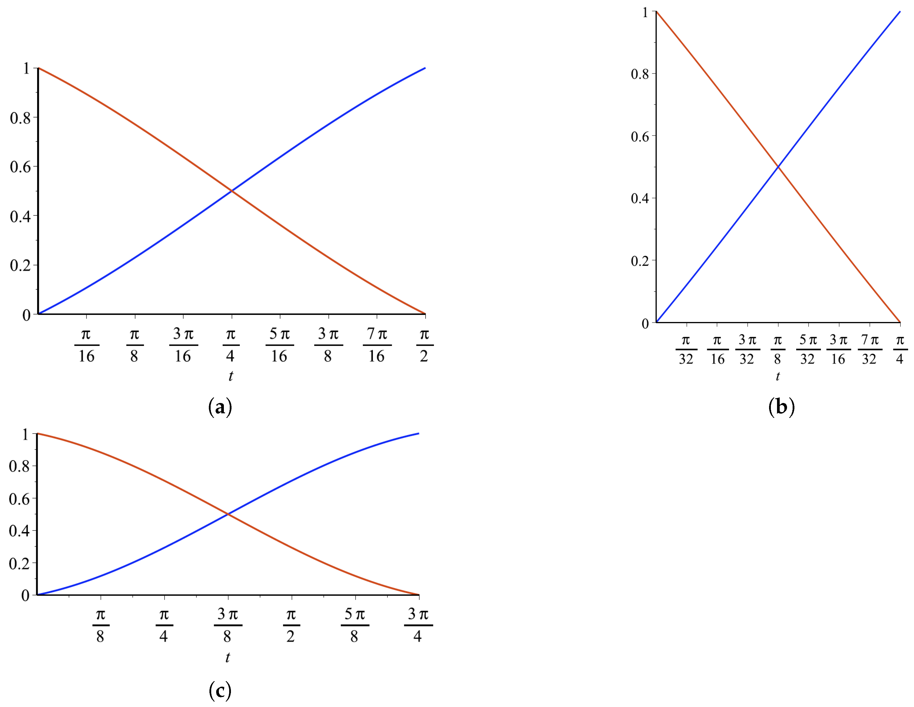
It can be easily checked that the functions in (11) satisfy $N_0^1(\alpha -t)=N_1^1\left(t\right)$, $t\in I_{\alpha }$ (see Figure 1 for an illustration of these functions). Moreover,

$${\mathsf{\Lambda }}_1\left(t\right)=(B_0^1\left(t\right),B_1^1\left(t\right))A_1\left(t\right),t\in I_{\alpha },$$

(12)

where $A_1\left(t\right)$ is defined by

$$A_1\left(t\right):=\left(\begin{array}{cc}{a}_0& b_0\\ a_1& b_1\end{array}\right)$$

with

$$a_0:=\frac{sin\alpha +sin(\alpha -t)-3sint}{2(sin(\alpha -t)-sint)},b_0:=a_0-1,a_1:=1-a_0,b_1:=2-a_0.$$

Figure 1. The functions $N_0^1,N_1^1$ (displayed in red and blue, respectively) for $\alpha =\frac{\pi }{4}$ (a), $\alpha =\frac{\pi }{2}$ (b) and $\alpha =\frac{3\pi }{4}$ (c).

Now, let us introduce the following functions defined on $I_{\alpha }$,

$$\begin{array}{c}\hfill (N_0^2,N_1^2,N_2^2):=(B_0^2,B_1^2,B_2^2)A_2,A_2:=\left(\begin{array}{ccc}\frac{1}{2}& \frac{1}{2}& 0\\ 0& 1& 0\\ 0& \frac{1}{2}& \frac{1}{2}\end{array}\right),\hfill \\ \hfill ({\overline{N}}_0^2,{\overline{N}}_1^2,{\overline{N}}_2^2):=(B_0^2,B_1^2,B_2^2){\overline{A}}_2,{\overline{A}}_2:=\left(\begin{array}{ccc}1& 0& 0\\ 0& 1& 0\\ 0& \frac{1}{2}& \frac{1}{2}\end{array}\right),\hfill \\ \hfill ({\widehat{N}}_0^2,{\widehat{N}}_1^2,{\widehat{N}}_2^2):=(B_0^2,B_1^2,B_2^2){\widehat{A}}_2,{\widehat{A}}_2:=\left(\begin{array}{ccc}\frac{1}{2}& \frac{1}{2}& 0\\ 0& 1& 0\\ 0& 0& 1\end{array}\right).\hfill \end{array}$$

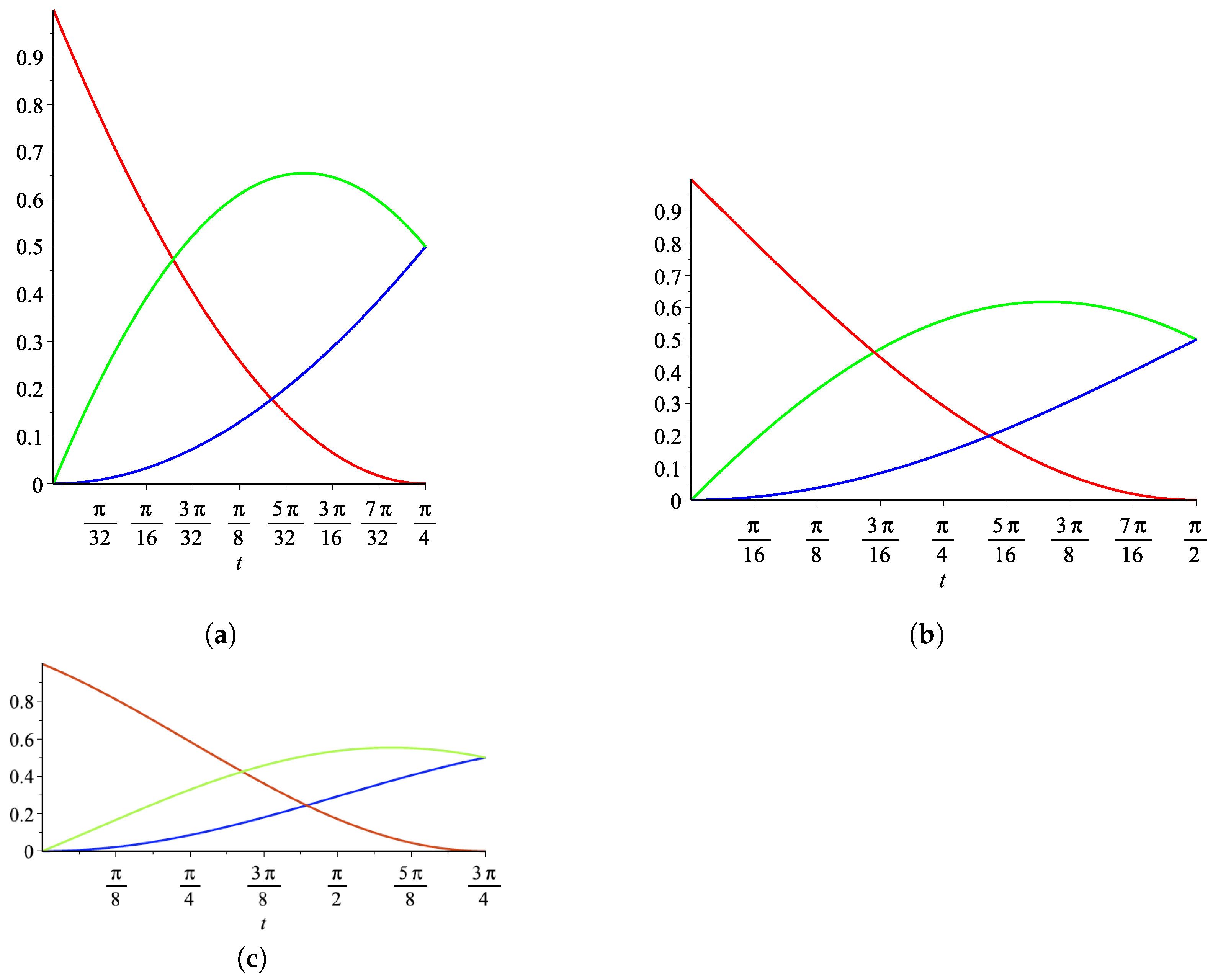
Clearly, the matrices $A_2,{\overline{A}}_2,{\widehat{A}}_2$ are nonsingular, stochastic and TP. Then, by Corollary 3.9 (iv) of [29], we can immediately deduce that the systems introduced in (13) are NTP bases of $U_2\left(I_{\alpha }\right)$. Figure 2, Figure 3 and Figure 4 illustrate the functions $N_i^2\left(t\right)$, ${\overline{N}}_i^2\left(t\right)$ and ${\widehat{N}}_i^2\left(t\right)$, respectively. On the other hand, by (13) and (5), we can obtain the following relations:

$$\begin{array}{c}(N_0^2\left(t\right),N_1^2\left(t\right),N_2^2\left(t\right))=(N_0^1\left(t\right),N_1^1\left(t\right)){\mathsf{\Lambda }}_2\left(t\right)A_2,t\in I_{\alpha },\hfill \\ ({\overline{N}}_0^2\left(t\right),{\overline{N}}_1^2\left(t\right),{\overline{N}}_2^2\left(t\right))=(N_0^1\left(t\right),N_1^1\left(t\right)){\mathsf{\Lambda }}_2\left(t\right){\overline{A}}_2,t\in I_{\alpha },\hfill \\ ({\widehat{N}}_0^2\left(t\right),{\widehat{N}}_1^2\left(t\right),{\widehat{N}}_2^2\left(t\right))=(N_0^1\left(t\right),N_1^1\left(t\right)){\mathsf{\Lambda }}_2\left(t\right){\widehat{A}}_2,t\in I_{\alpha }.\hfill \end{array}$$

(13)

Figure 2. The functions $N_0^2,N_1^2,N_2^2$ (displayed in red, green and blue, respectively) for $\alpha =\frac{\pi }{4}$ (a), $\alpha =\frac{\pi }{2}$ (b) and $\alpha =\frac{3\pi }{4}$ (c).

Figure 3. The functions ${\overline{N}}_0^2,{\overline{N}}_1^2,{\overline{N}}_2^2$ (displayed in red, green and blue, respectively) for $\alpha =\frac{\pi }{4}$ (a), $\alpha =\frac{\pi }{2}$ (b) and $\alpha =\frac{3\pi }{4}$ (c).

Figure 4. The functions ${\widehat{N}}_0^2,{\widehat{N}}_1^2,{\widehat{N}}_2^2$ (displayed in red, green and blue, respectively) for $\alpha =\frac{\pi }{4}$ (a), $\alpha =\frac{\pi }{2}$ (b) and $\alpha =\frac{3\pi }{4}$ (c).

The following result collects important properties of the functions in (13).

Theorem 2.

The following properties hold for the functions defined in (13).

1.

$N_0^2(\alpha -t)=N_2^2\left(t\right)$, $N_1^2(\alpha -t)=N_1^2\left(t\right)$, $t\in I_{\alpha }$.

2.

$$\begin{gathered} N_0^2\left(0\right)=\frac{1}{2},N_1^2\left(0\right)=\frac{1}{2},N_2^2\left(0\right)=0, \\ {N}_0^2\left(\alpha \right)=0,N_1^2\left(\alpha \right)=\frac{1}{2},N_2^2\left(\alpha \right)=\frac{1}{2}. \end{gathered}$$

3.

$$\begin{gathered} {\left(N_0^2\right)}^{\prime }\left(0\right)=-\frac{1}{2}cot\left(\frac{\alpha }{2}\right),{\left(N_1^2\right)}^{\prime }\left(0\right)=\frac{1}{2}cot\left(\frac{\alpha }{2}\right),{\left(N_2^2\right)}^{\prime }\left(0\right)=0. \\ {\left(N_0^2\right)}^{\prime }\left(\alpha \right)=0,{\left(N_1^2\right)}^{\prime }\left(\alpha \right)=-\frac{1}{2}cot\left(\frac{\alpha }{2}\right),{\left(N_2^2\right)}^{\prime }\left(\alpha \right)=\frac{1}{2}cot\left(\frac{\alpha }{2}\right). \end{gathered}$$

4.

$$\begin{gathered} {\overline{N}}_0^2\left(0\right)=1,{\overline{N}}_1^2\left(0\right)=0,{\overline{N}}_2^2\left(0\right)=0 \\ {\overline{N}}_0^2\left(\alpha \right)=0,{\overline{N}}_1^2\left(\alpha \right)=\frac{1}{2},{\overline{N}}_2^2\left(\alpha \right)=\frac{1}{2}. \end{gathered}$$

5.

$$\begin{gathered} {\left({\overline{N}}_0^2\right)}^{\prime }\left(0\right)=-cot\left(\frac{\alpha }{2}\right),{\left({\overline{N}}_1^2\right)}^{\prime }\left(0\right)=cot\left(\frac{\alpha }{2}\right),{\left({\overline{N}}_2^2\right)}^{\prime }\left(0\right)=0. \\ {\left({\overline{N}}_0^2\right)}^{\prime }\left(\alpha \right)=0,{\left({\overline{N}}_1^2\right)}^{\prime }\left(\alpha \right)=-\frac{1}{2}cot\left(\frac{\alpha }{2}\right),{\left({\overline{N}}_2^2\right)}^{\prime }\left(\alpha \right)=\frac{1}{2}cot\left(\frac{\alpha }{2}\right). \end{gathered}$$

6.

$$\begin{gathered} {\widehat{N}}_0^2\left(0\right)=\frac{1}{2},{\widehat{N}}_1^2\left(0\right)=\frac{1}{2},{\widehat{N}}_2^2\left(0\right)=0. \\ {\widehat{N}}_0^2\left(\alpha \right)=0,{\widehat{N}}_1^2\left(\alpha \right)=0,{\widehat{N}}_2^2\left(\alpha \right)=1. \end{gathered}$$

7.

$$\begin{gathered} {\left({\widehat{N}}_0^2\right)}^{\prime }\left(0\right)=-\frac{1}{2}cot\left(\frac{\alpha }{2}\right),{\left({\widehat{N}}_1^2\right)}^{\prime }\left(0\right)=\frac{1}{2}cot\left(\frac{\alpha }{2}\right),{\left({\widehat{N}}_2^2\right)}^{\prime }\left(0\right)=0. \\ {\left({\widehat{N}}_0^2\right)}^{\prime }\left(\alpha \right)=0,{\left({\widehat{N}}_1^2\right)}^{\prime }\left(\alpha \right)=-cot\left(\frac{\alpha }{2}\right),{\left({\widehat{N}}_2^2\right)}^{\prime }\left(\alpha \right)=cot\left(\frac{\alpha }{2}\right). \end{gathered}$$

8.

${\sum }_{i=0}^2{N}_i^2\left(t\right)=1,{\sum }_{i=0}^2{\overline{N}}_i^2\left(t\right)=1,{\sum }_{i=0}^2{\widehat{N}}_i^2\left(t\right)=1,t\in I_{\alpha }$.

For $p\in \mathbb{N}$, $p\ge 2$, we consider the equally spaced partitions

$$\mathit{\pi }={\left\{u_i\right\}}_{i=0}^{p+3}={\left\{i\alpha \right\}}_{i=0}^{p+3},$$

(14)

and

$$\mathit{\mu }={\left\{u_i\right\}}_{i=0}^{p+3},$$

(15)

with $u_0=u_1=u_2=0$, $u_i=(i-2)\alpha$, for $i=3,\dots ,p+1$, and $u_{p+1}=u_{p+2}=u_{p+3}=$$(p-1)\alpha$ for the partition $\mathit{\mu }$ in (15). We thus define the piecewise functions on either partition $\mathit{\pi }$ or $\mathit{\mu }$.

$$\begin{array}{ccc}\hfill N_{i,0}\left(u\right)& :=& \left\{\begin{array}{cc}1,\hfill & u\in [u_i,u_{i+1}),\hfill \\ 0,\hfill & \mathrm{else},\hfill \end{array}\right.\hfill \end{array}$$

(16)

$$\begin{array}{ccc}\hfill N_{i,1}\left(u\right)& :=& \left\{\begin{array}{cc}{N}_1^1(u-u_i),\hfill & u\in [u_i,u_{i+1}),\hfill \\ N_0^1(u-u_{i+1}),\hfill & u\in [u_{i+1},u_{i+2}),\hfill \\ 0,\hfill & \mathrm{else},\hfill \end{array}\right.\hfill \end{array}$$

(17)

$$\begin{array}{ccc}\hfill N_{i,2}\left(u\right)& :=& \left\{\begin{array}{cc}{N}_2^2(u-u_i),\hfill & u\in [u_i,u_{i+1}),\hfill \\ N_1^2(u-u_{i+1}),\hfill & u\in [u_{i+1},u_{i+2}),\hfill \\ N_0^2(u-u_{i+2}),\hfill & u\in [u_{i+2},u_{i+3}),\hfill \\ 0,\hfill & \mathrm{else},\hfill \end{array}\right.\hfill \end{array}$$

(18)

for $i=0,\dots ,p$. On the partition $\mathit{\mu }$, we also define

$$\begin{array}{ccc}\hfill {\tilde{N}}_{0,2}\left(u\right)& :=& \left\{\begin{array}{cc}{\overline{N}}_0^2(u-u_2),\hfill & u\in [u_2,u_3),\hfill \\ 0,\hfill & \mathrm{else},\hfill \end{array}\right.\hfill \\ \hfill {\tilde{N}}_{1,2}\left(u\right)& :=& \left\{\begin{array}{cc}{\overline{N}}_1^2(u-u_2),\hfill & u\in [u_2,u_3),\hfill \\ N_0^2(u-u_3),\hfill & u\in [u_3,u_4),\hfill \\ 0,\hfill & \mathrm{else},\hfill \end{array}\right.\hfill \end{array}$$

$$\begin{array}{ccc}\hfill {\tilde{N}}_{p-1,2}\left(u\right)& :=& \left\{\begin{array}{cc}{N}_2^2(u-u_{p-1}),\hfill & u\in [u_{p-1},u_p),\hfill \\ {\widehat{N}}_1^2(u-u_p),\hfill & u\in [u_p,u_{p+1}),\hfill \\ 0,\hfill & \mathrm{else},\hfill \end{array}\right.\hfill \end{array}$$

(19)

$$\begin{array}{ccc}\hfill {\tilde{N}}_{p,2}\left(u\right)& :=& \left\{\begin{array}{cc}{\widehat{N}}_2^2(u-u_p),\hfill & u\in [u_p,u_{p+1}),\hfill \\ 0,\hfill & \mathrm{else}.\hfill \end{array}\right.\hfill \end{array}$$

(20)

Figure 5 illustrates the functions $N_{i,2}$, ${\tilde{N}}_{1,2}$ and ${\tilde{N}}_{p-1,2}$.

Figure 5. The functions $N_{i,2}$ (a), ${\tilde{N}}_{1,2}$ (b), ${\tilde{N}}_{p-1,2}$ (c) for $\alpha =\frac{\pi }{4}$.

By construction, the following properties hold for the above functions.

Proposition 1.

The functions defined by (16)–(20) have the following properties:

(N1)

For $j\in \{1,2\}$, $N_{i,j}\left(u\right)$ is a piecewise trigonometric function of the space $U_j\left(I_{\alpha }\right)$ and, for $i=0,1,p-1,p$, ${\tilde{N}}_{i,2}\left(u\right)$ is a piecewise trigonometric function of the space $U_2\left(I_{\alpha }\right)$.

(N2)

For all applicable indices,

$$N_{i,j}\left(u\right)\left\{\begin{array}{cc}>0,\hfill & u\in (u_i,u_{i+j+1}),\hfill \\ =0,\hfill & \mathrm{else}.\hfill \end{array}\right.$$

For $i=0,1,p-1,p$,

$${\tilde{N}}_{i,2}\left(u\right)\left\{\begin{array}{cc}>0,\hfill & u\in (u_i,u_{i+3}),\hfill \\ =0,\hfill & else.\hfill \end{array}\right.$$

In fact, $N_{i,j}\left(u\right)$ has the minimal support $[u_i,u_{i+j+1}]$ and ${\tilde{N}}_{i,2}\left(u\right)$ has the minimal support $[u_i,u_{i+3}]$.

(N3)

$N_{i,j}{\left(u\right)|}_{[u_l,u_{l+1}]}\ne 0$ for $i=l-j,\dots ,l$.

(N4)

For $j\in \{1,2\}$, $N_{i,j}\left(u\right)$ are symmetrical with respect to the middle of their supports and they can be obtained by translation, i.e., $N_{i,j}\left(u\right)=N_{0,j}(u-u_i)$.

(N5)

Over the partition $\mathit{\pi }$,

$${\displaystyle \sum _{i=0}^{p+2-j}{N}_{i,j}\left(u\right)=1,u\in [u_2,u_{p+1}].}$$

(N6)

Over the partition $\mathit{\mu }$,

$${\displaystyle \sum _{i=0}^{p+2-j}{N}_{i,j}\left(u\right)=1,u\in [u_2,u_{p+1}],}$$

where $N_{i,2}={\tilde{N}}_{i,2}$ for $i=0,1,p-1,p$.

(N7)

On the partitions $\mathit{\pi }$ and $\mathit{\mu }$, the functions $N_{i,j}\left(u\right)$ for $i=0,\dots ,p+2-j$ and $j=0,1,2$, and ${\tilde{N}}_{i,2}\left(u\right)$ for $i=0,1,p-1,p$ are $C^{j-mult\left(u_k\right)}$-continuous, where $mult\left(u_k\right)$ is the multiplicity of the knot $u_k$ in the support of the corresponding function.

Let us note that the restriction of the functions $N_{i,2,\mathit{\mu }}$, $i=0,\dots ,p$, to each interval $[u_k,u_{k+1}]$, $k=0,\dots ,p$, generates $U_2\left(I_{\alpha }\right)$, which is a Chebyshev space (see [2]). Therefore, $(N_{0,2,\mathit{\mu }},\dots ,N_{p,2,\mathit{\mu }})$ generates a space $\mathcal{S}$ of Chebyshevian splines with a totally positive basis (see Chapter 9 of [34]). In addition, the system also satisfies

$$\underset{u\to u_j^{+}}{lim}{N}_{k,2,\mathit{\mu }}\left(u\right)/N_{j,2,\mathit{\mu }}\left(u\right)=0,\underset{u\to u_{k+3}^{-}}{lim}{N}_{j,2,\mathit{\mu }}\left(u\right)/N_{k,2,\mathit{\mu }}\left(u\right)=0,$$

whenever $j<k$. Then, by Theorem 3.2 of Chapter 4 of [13], $(N_{0,2,\mathit{\mu }},\dots ,N_{p,2,\mathit{\mu }})$ is the normalized B-basis of $\mathcal{S}$. This fact implies optimal shape-preserving properties (see [29] and Chapter 4 of [13]). Due to the analogy to the well-known polynomial B-splines, we will say that the functions $N_{i,2,\mathit{\mu }}$, $i=0,\dots ,p$, are $T_2$-B-splines.

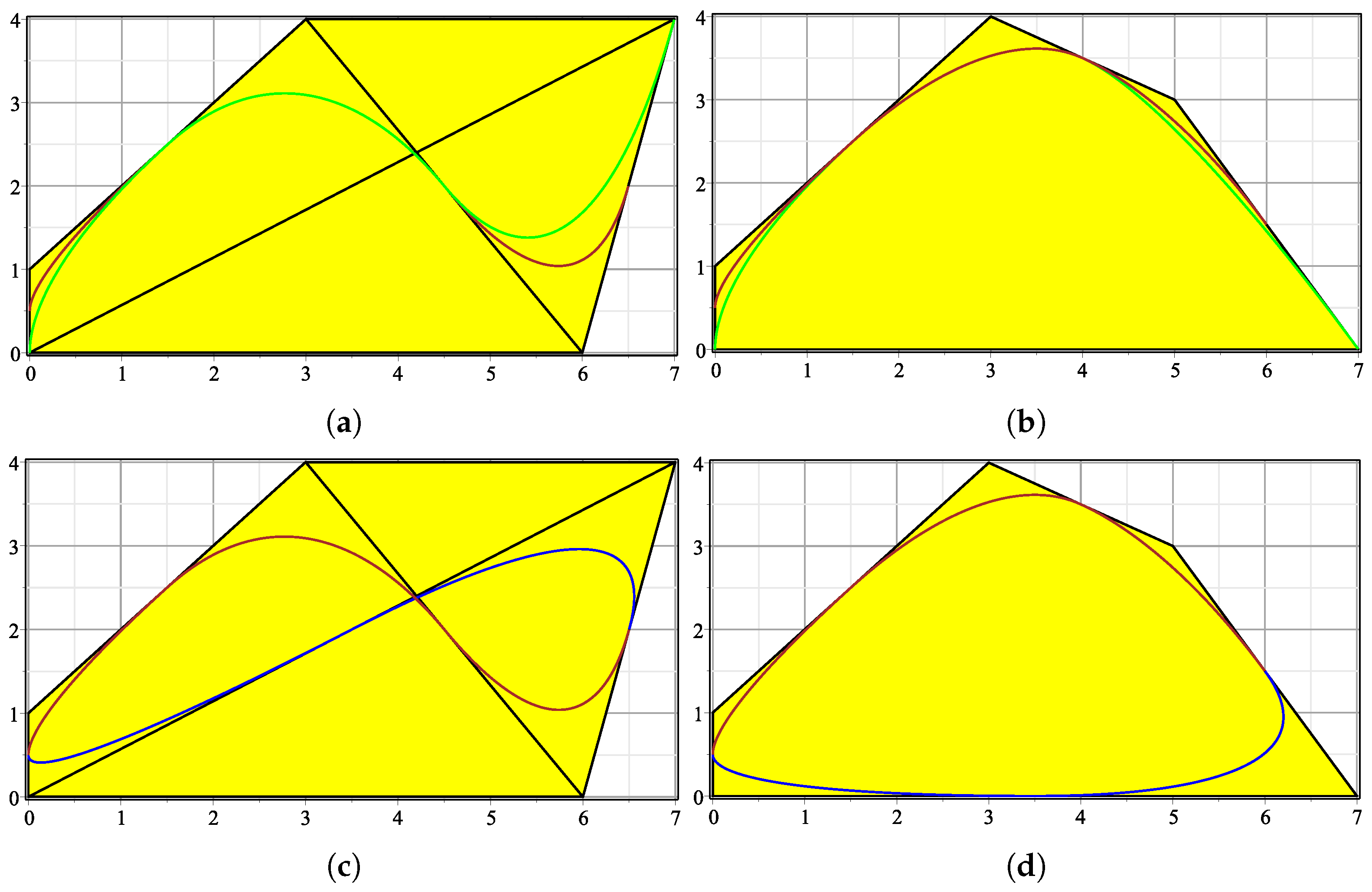
Now, we can define trigonometric piecewise curves (see Figure 6 for an illustration).

Figure 6. Open (red), clamped (green) and closed (red and blue) $T_2$-B-spline curves with control points $s_0=(0,0)$, $s_1=(0,1)$, $s_2=(3,4)$, $s_3=(6,0)$, $s_4=(7,4)$ (first column), respectively, $s_0=(0,0)$, $s_1=(0,1)$, $s_2=(3,4)$, $s_3=(5,3)$, $s_4=(7,0)$ (second column). Figures (a,b) show the open and clamped curves, figures (c,d) show the open and closed curves; the closed control polygon and convex hull of the control points are also displayed in yellow.

Definition 2.

For given $p,d\in \mathbb{N}$, $p\ge 2$, let $s_i\in {\mathbb{R}}^d$, $i=0,\dots ,p$, and the knot partitions $\mathit{\pi }$, $\mathit{\mu }$ defined in (14) and (15), respectively, are defined as follows.

(a)

The functions $N_{i,j,\mathit{\pi }}\left(u\right)=N_{i,j}\left(u\right)$ for $i=0,\dots ,p+2-j$ and $j=0,1,2$ are called normalized $T_2$-B-splines over the partition $\mathit{\pi }$ and the functions $N_{i,j,\mathit{\mu }}\left(u\right)=N_{i,j}\left(u\right)$ for $i=0,\dots ,p+2-j$ and $j=0,1$, $N_{i,2,\mathit{\mu }}\left(u\right)=N_{i,2}\left(u\right)$ for $i=2,\dots ,p-2$ and $N_{i,2,\mathit{\mu }}\left(u\right)={\tilde{N}}_{i,2}\left(u\right)$ for $i=0,1,p-1,p$ are called normalized $T_2$-B-splines over the partition $\mathit{\mu }$.

(b)

The parametric curve

$$s\left(u\right):=\sum _{i=0}^p{s}_i{N}_{i,2,\mathit{\pi }}\left(u\right),u\in [u_2,u_{p+1}),$$

(21)

is called a $T_2$-B-spline curve (with respect to the partition $\mathit{\pi }$) with the control points $s_0,\dots ,s_p$. In particular, for $p=m$, with $m\in \mathbb{N}$, $m\ge 2$, we refer to this curve as an open $T_2$-B-spline curve, and for $p=m+2$ and $s_{m+1}=s_0$, $s_{m+2}=s_1$, we have a closed $T_2$-B-spline curve.

(c)

For $p=m$, with $m\in \mathbb{N},m\ge 2$, the curve

$$s\left(u\right):=\sum _{i=0}^m{s}_i{N}_{i,2,\mathit{\mu }}\left(u\right),u\in [u_2,u_{m+1})$$

(22)

is called a clamped $T_2$-B-spline curve (with respect to the partition $\mathit{\mu }$) with the control points $s_0,\dots ,s_m$.

From the properties of their blending functions given in Proposition 1, the following properties of $T_2$-B-spline curves can easily be derived.

Proposition 2.

(C1)

The relation between the curve $s\left(u\right)$ and its control points $s_0,\dots ,s_p$ is affinely invariant, i.e., the $T_2$-B-spline curve constructed from images of the control points $s_0,\dots ,s_p$ under an affine transformation is identical to the image of the curve $s\left(u\right)$ under the same affine transformation.

(C2)

The curve $s\left(u\right)$ is locally controlled, i.e., moving a control point $s_l$ only modifies the curve for $u\in [u_l,u_{l+3})$. Moreover, for $\mathit{\tau }=\mathit{\pi }$ or $\mathit{\tau }=\mathit{\mu }$, we have

$${s\left(u\right)|}_{u\in [u_l,u_{l+1})}=\sum _{i=l-2}^l{s}_i{N}_{i,2,\mathit{\tau }}\left(u\right),$$

(23)

and the curve $s\left(u\right)$ lies in the convex hull of its control points. More precisely,

$${s\left(u\right)|}_{u\in [u_l,u_{l+1})}\subset \mathsf{\Delta }(s_{l-2},s_{l-1},s_l),$$

(24)

where $\mathsf{\Delta }(s_{l-2},s_{l-1},s_l)$ is the triangle generated by the points $s_{l-2},s_{l-1},s_l$.

(C3)

For a clamped $T_2$-B-spline curve, we have end-point and end-tangent interpolation, namely

$$\begin{array}{ccc}& & s\left(u_1\right)=s\left(0\right)=s_0,s\left(u_{m+1}\right)=s_m,\hfill \\ & & s^{\prime }\left(0\right)=cot\left(\frac{\alpha }{2}\right)(s_1-s_0),s^{\prime }\left(u_{m+1}\right)=cot\left(\frac{\alpha }{2}\right)(s_m-s_{m-1}).\hfill \end{array}$$

(C4)

If three control points $s_{l-2},s_{l-1},s_l$ are collinear, the $T_2$-B-spline curve $s\left(u\right)$ contains part of the straight line through $s_{l-2},s_{l-1},s_l$.

(C5)

The straight line through $s_{l-2},s_{l-1}$ is tangent to the $T_2$-B-spline curve $s\left(u\right)$ in the point $s\left(u_l\right)$, i.e., every leg of the control polygon is tangent to the curve.

The normalized $T_2$-B-spline functions from Definition 2a can be conveniently generated by a Cox–de Boor-like recurrence relation as follows.

Theorem 3.

By introducing the following abbreviations

$$\begin{array}{c}{\gamma }_{i,1}\left(u\right):=\frac{sin\left(\frac{u-u_i}{2}\right)cos\left(\frac{\alpha -u+u_i}{2}\right)}{sin\left(\frac{\alpha }{2}\right)},\hfill \\ {\gamma }_{i,2}\left(u\right):=\frac{sin(u-u_{i+1}+\alpha )-sin(u-u_{i+1})-sin\left(\alpha \right)}{2sin(u-u_{i+1})(cos\left(\alpha \right)-1)},\hfill \end{array}$$

(25)

and considering the piecewise functions $N_{i,0}\left(u\right)$ from (16), we obtain

$$N_{i,j,\mathit{\tau }}\left(u\right)={\gamma }_{i,j}\left(u\right)N_{i,j-1,\mathit{\tau }}\left(u\right)+{\rho }_{i,j}\left(u\right)N_{i+1,j-1,\mathit{\tau }}\left(u\right).$$

(26)

Herein, the partition, the coefficients and the index range vary according to the type of $T_2$-B-spline curve (open, closed, clamped) in the following way:

(a)

For $\mathit{\tau }=\mathit{\pi }$, $i=0,\dots ,p+2-j$, $j=1,2$ and

$${\rho }_{i,j}\left(u\right)=1-{\gamma }_{i+1,j}\left(u\right),$$

(27)

and the recurrence relation (26) generates the blending functions of an open (respectively, closed) $T_2$-B-spline curve for $p=m$ (respectively, for $p=m+2$).

(b)

For $\mathit{\tau }=\mathit{\mu }$, the coefficients ${\gamma }_{i,1}\left(u\right)$ (respectively, ${\gamma }_{i,2}\left(u\right)$) are defined as in (25) for $i=0,\dots ,m+2$ (respectively, $i=2,\dots ,m-2$). The remaining coefficients are defined as follows:

$$\begin{array}{ccc}\hfill {\rho }_{i,1}\left(u\right)& =& 1-{\gamma }_{i+1,1}\left(u\right),fori=0,\dots ,m+1,\hfill \\ \hfill {\rho }_{i,2}\left(u\right)& =& 1-{\gamma }_{i+1,2}\left(u\right),fori=2,\dots ,m-3,\hfill \\ \hfill {\rho }_{m-2,2}\left(u\right)& =& 1-\frac{sin(u-u_m+\alpha )-sin(u-u_m)-sin\left(\alpha \right)}{2sin(u-u_m)(cos\left(\alpha \right)-1)},\hfill \\ \hfill {\gamma }_{0,2}\left(u\right)& =& 0,\hfill \\ \hfill {\rho }_{0,2}\left(u\right)& =& \frac{{\overline{N}}_0^2(u-u_2)}{N_0^1(u-u_2)},\hfill \\ \hfill {\rho }_{1,2}\left(u\right)& =& \frac{{\widehat{N}}_0^2(u-u_3)}{N_0^1(u-u_3)},\hfill \\ \hfill {\gamma }_{1,2}\left(u\right)& =& \frac{{\overline{N}}_1^2(u-u_2)-{\rho }_{1,2}\left(u\right)N_1^1(u-u_2)}{N_0^1(u-u_2)},\hfill \\ \hfill {\gamma }_{m-1,2}\left(u\right)& =& \frac{{\overline{N}}_2^2(u-u_{m-1})}{N_1^1(u-u_{m-1})},\hfill \\ \hfill {\rho }_{m-1,2}\left(u\right)& =& \frac{{\widehat{N}}_1^2(u-u_m)-{\gamma }_{m-1,2}\left(u\right)N_0^1(u-u_m)}{N_1^1(u-u_m)},\hfill \\ \hfill {\gamma }_{m,2}\left(u\right)& =& \frac{{\widehat{N}}_2^2(u-u_m)}{N_1^1(u-u_m)},\hfill \\ \hfill {\rho }_{m,2}\left(u\right)& =& 0.\hfill \end{array}$$

Thus, the recurrence relation (26) generates the blending functions of a clamped $T_2$-B-spline curve.

Proof. 

According to (13), we have

$$\begin{array}{c}{N}_0^2(u-u_{i+2})=\frac{1}{2}(1-{\lambda }_0^0(u-u_{i+2}))N_0^1(u-u_{i+2}),\hfill \\ N_1^2(u-u_{i+1})=\frac{1}{2}(1+{\lambda }_0^0(u-u_{i+1}))N_0^1(u-u_{i+1})+(1-\frac{1}{2}{\lambda }_1^0(u-u_{i+1}))N_1^1(u-u_{i+1}),\hfill \\ N_2^2(u-u_i)=\frac{1}{2}{\lambda }_1^0(u-u_i)N_1^1(u-u_i).\hfill \end{array}$$

The following identities can be easily checked

$$\begin{array}{c}\frac{1}{2}(1-{\lambda }_0^0(u-u_{i+2}))=1-\frac{1}{2}{\lambda }_1^0(u-u_{i+1}),\hfill \\ \frac{1}{2}(1+{\lambda }_0^0(u-u_{i+1}))=\frac{1}{2}{\lambda }_1^0(u-u_i),\hfill \end{array}$$

(28)

and then, for $j=2$, we obtain the recurrence relation (26) for all i, in the open and closed cases, and for $i=2,\dots ,m-2$, in the clamped case. For $j=1$, Equation (26) is obtained in a straightforward manner by (11), (16) and (17). The remaining equations from (26) in the clamped case for $j=2$ are readily obtained by (17) and (20). □

Thanks to this recurrence relation, we immediately obtain a de Boor-like or corner cutting algorithm for the evaluation of the $T_2$-B-spline curves.

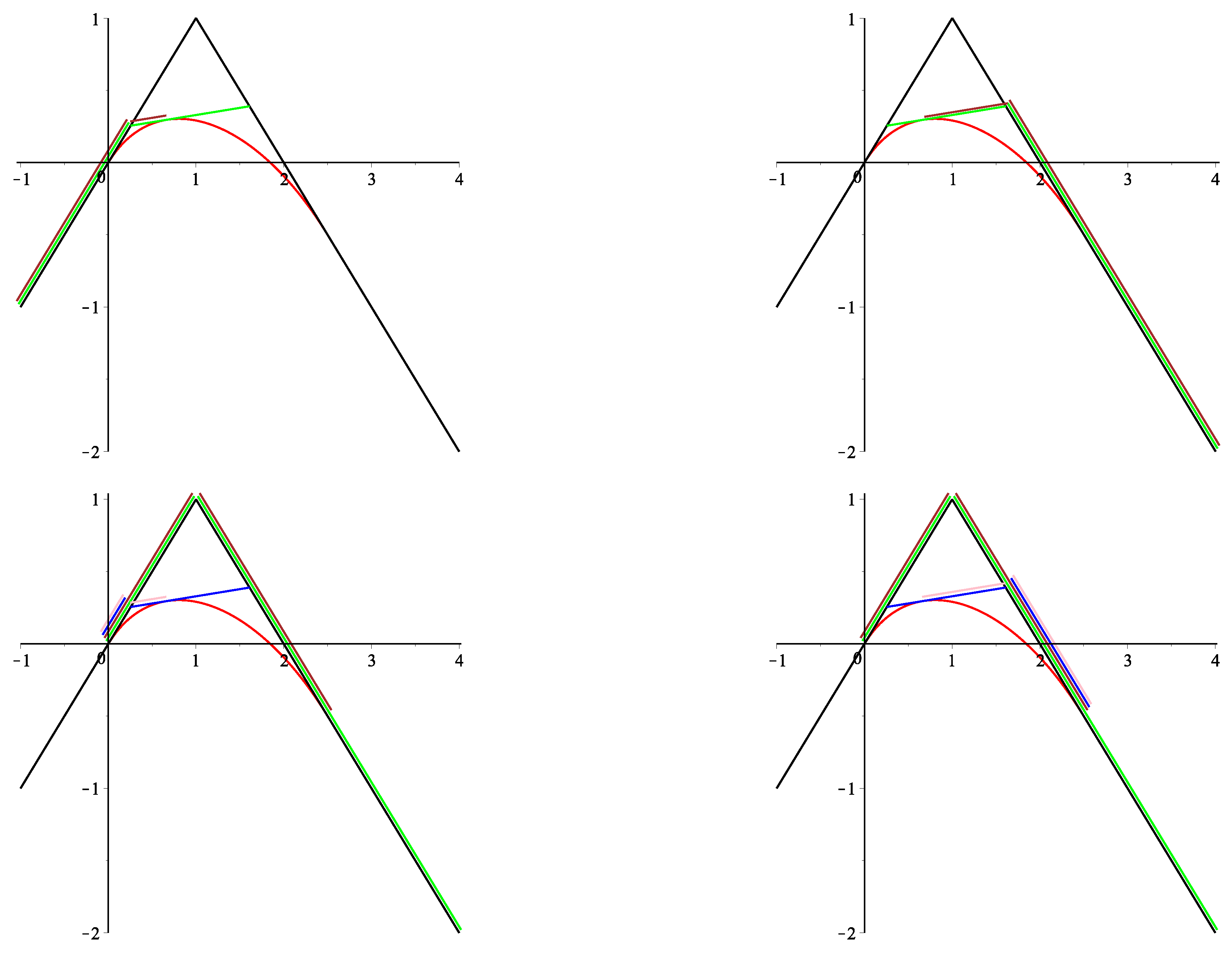
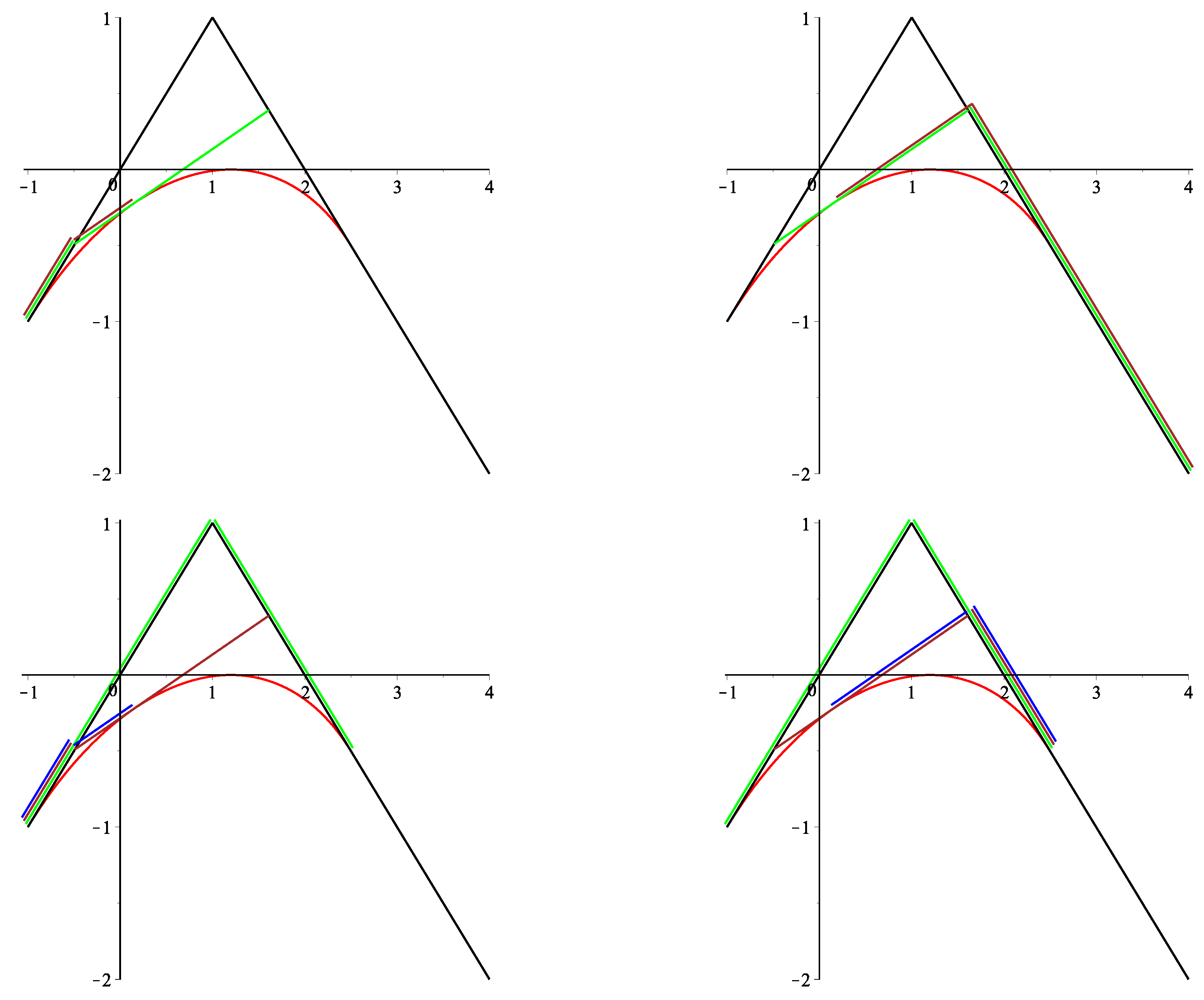
Theorem 4.

Given an open, closed or clamped $T_2$-B-spline curve over the partition $\mathit{\tau }=\mathit{\pi }$ or $\mathit{\tau }=\mathit{\mu }$, according to Definition 2,

$$s\left(u\right)=\sum _{i=0}^p{s}_i{N}_{i,2,\mathit{\tau }}\left(u\right),u\in [u_2,u_{p+1}),$$

(29)

the curve point $s\left(u\right)$ for a parameter $u\in [u_l,u_{l+1})$ is obtained as

$$s\left(u\right)=s_l^2,$$

where

$$s_i^k=s_i^{k-1}{\gamma }_{i,3-k}\left(u\right)+s_{i-1}^{k-1}{\rho }_{i-1,3-k}\left(u\right)$$

for $k=1,2$ and $i=l-2+k,\dots ,l$.

Remark 1.

The de Boor-like algorithm from Theorem 4 may be written in matrix form as follows

$$\left(\begin{array}{c}{s}_{l-2}^0\\ s_{l-1}^1\\ s_l^2\end{array}\right)=\overline{L}\left(\begin{array}{c}{s}_{l-2}^0\\ s_{l-1}^0\\ s_l^0\end{array}\right),\left(\begin{array}{c}{s}_l^2\\ s_l^1\\ s_l^0\end{array}\right)=\overline{U}\left(\begin{array}{c}{s}_{l-2}^0\\ s_{l-1}^0\\ s_l^0\end{array}\right),$$

(30)

where $\overline{L}={\overline{L}}_1{\overline{L}}_0$ and $\overline{U}={\overline{U}}_1{\overline{U}}_0$ with

$${\overline{L}}_0=\left(\begin{array}{ccc}1& 0& 0\\ {\rho }_{l-2,2}& {\gamma }_{l-1,2}& 0\\ 0& {\rho }_{l-1,2}& {\gamma }_{l,2}\end{array}\right),{\overline{L}}_1=\left(\begin{array}{ccc}1& 0& 0\\ 0& 1& 0\\ 0& {\rho }_{l-1,1}& {\gamma }_{l,1}\end{array}\right),$$

and

$${\overline{U}}_0=\left(\begin{array}{ccc}{\rho }_{l-2,2}& {\gamma }_{l-1,2}& 0\\ 0& {\rho }_{l-1,2}& {\gamma }_{l,2}\\ 0& 0& 1\end{array}\right),{\overline{U}}_1=\left(\begin{array}{ccc}{\rho }_{l-1,1}& {\gamma }_{l,1}& 0\\ 0& 1& 0\\ 0& 0& 1\end{array}\right).$$

For an illustration, see Figure 7 and Figure 8, first row.

Figure 7. Successive intermediate control polygons (in the color order black-green-brown (first row) respectively, black-green-brown-blue-pink (second row)) generated by the de Boor-like algorithm from Theorem 4 (first row) and by the alternative corner cutting algorithm from Remark 2 (second row) for a segment of an open or closed $T_2$-B-spline curve or an inner segment of a clamped $T_2$-B-spline curve. The first (respectively, second) column illustrates the left (respectively, right) factorization from Equations (30) and (31).

Figure 8. Successive intermediate control polygons (in the color order black-green-brown (first row) respectively black-green-brown-blue (second row)) generated by the de Boor-like algorithm from Theorem 4 (first row) and by the alternative corner cutting algorithm from Remark 2 (second row) for the initial segment of a clamped $T_2$-B-spline curve for $\alpha =\frac{\pi }{2}$. The first and second columns illustrate the left and right factorizations, respectively, from Equations (30) and (32).

Remark 2.

Additionally to the above de Boor-like corner cutting algorithm, the $T_2$-B-spline curves also admit the following corner cutting algorithm. Considering a segment of an open or closed $T_2$-B-spline curve (see Definition 2b) for the curve parameter $u\in [u_l,u_{l+1})$, $l\in \{2,\dots ,p\}$, or an inner segment of a clamped $T_2$-B-spline curve (see Definition 2c) for the curve parameter $u\in [u_l,u_{l+1})$, $l\in \{3,\dots ,m-1\}$, we have

$${s\left(u\right)|}_{u\in [u_l,u_{l+1})}=(N_0^2(u-u_l),N_1^2(u-u_l),N_2^2(u-u_l))\left(\begin{array}{c}{s}_{l-2}^0\\ s_{l-1}^0\\ s_l^0\end{array}\right).$$

According to (13) and Definition 1, the points

$$\left(\begin{array}{c}{p}_{l,0}^0\\ p_{l,1}^0\\ p_{l,2}^0\end{array}\right)=A_2\left(\begin{array}{c}{s}_{l-2}^0\\ s_{l-1}^0\\ s_l^0\end{array}\right)$$

are thus the control points of a $T_2$-curve. Considering the factorization $A_2={\overline{A}}_2{\widehat{A}}_2={\widehat{A}}_2{\overline{A}}_2$ of the matrix $A_2$ and applying the de Casteljau-like algorithm from (10), the corner cutting algorithm may be written in matrix form as follows (analogously, the factorization $A_2={\widehat{A}}_2{\overline{A}}_2$ can be used):

$$\left(\begin{array}{c}{p}_{l,0}^0\\ p_{l,0}^1\\ p_{l,0}^2\end{array}\right)=L_1{L}_0{\overline{A}}_2{\widehat{A}}_2\left(\begin{array}{c}{s}_{l-2}^0\\ s_{l-1}^0\\ s_l^0\end{array}\right),\left(\begin{array}{c}{p}_{l,0}^2\\ p_{l,1}^1\\ p_{l,2}^0\end{array}\right)=U_1{U}_0{\overline{A}}_2{\widehat{A}}_2\left(\begin{array}{c}{s}_{l-2}^0\\ s_{l-1}^0\\ s_l^0\end{array}\right),$$

(31)

with the matrices $L_i,U_i$ from (10) and $t=u-u_l$. For the initial and final segments of a clamped $T_2$-B-spline curve, i.e., for the curve parameter $u\in [u_l,u_{l+1})$, for $l\in \{2,m\}$, we obtain

$${s\left(u\right)|}_{u\in [u_2,u_3)}=({\overline{N}}_0^2(u-u_2),{\overline{N}}_1^2(u-u_2),{\overline{N}}_2^2(u-u_2))\left(\begin{array}{c}{s}_0^0\\ s_1^0\\ s_2^0\end{array}\right),$$

for $l=2$, and

$${s\left(u\right)|}_{u\in [u_m,u_{m+1})}=({\widehat{N}}_0^2(u-u_m),{\widehat{N}}_1^2(u-u_m),{\widehat{N}}_2^2(u-u_m))\left(\begin{array}{c}{s}_{m-2}^0\\ s_{m-1}^0\\ s_m^0\end{array}\right),$$

for $l=m$, and thus

$$\left(\begin{array}{c}{p}_{l,0}^0\\ p_{l,0}^1\\ p_{l,0}^2\end{array}\right)=L_1{L}_0{A}_2^l\left(\begin{array}{c}{s}_{l-2}^0\\ s_{l-1}^0\\ s_l^0\end{array}\right),\left(\begin{array}{c}{p}_{l,0}^2\\ p_{l,1}^1\\ p_{l,2}^0\end{array}\right)=U_1{U}_0{A}_2^l\left(\begin{array}{c}{s}_{l-2}^0\\ s_{l-1}^0\\ s_l^0\end{array}\right),$$

(32)

for $l\in \{2,m\}$, and $A_2^2={\overline{A}}_2$, $A_2^m={\widehat{A}}_2$. For an illustration, see Figure 7 and Figure 8, second row. Comparing this corner cutting algorithm with the de Boor-like algorithm from Theorem 4 and Remark 1, we observe that $s_l^2=p_{l,0}^2$, $s_{l-1}^1=p_{l,0}^1$, $s_l^1=p_{l,1}^1$, but $s_{l-2}^0\ne p_{l,0}^0$, and $s_l^0\ne p_{l,2}^0$ in the case of a segment of an open or closed $T_2$-B-spline curve or of an inner segment of a clamped $T_2$-B-spline curve. In the case of the initial or final segment of a clamped $T_2$-B-spline curve, we have $s_2^2=p_{2,0}^2$, $s_1^1=p_{2,0}^1$, $s_2^1=p_{2,1}^1$, $s_0^0=p_{2,0}^0$, but $s_2^0\ne p_{2,2}^0,$ respectively, $s_m^2=p_{m,0}^2$, $s_{m-1}^1=p_{m,0}^1$, $s_m^1=p_{m,1}^1$, $s_m^0=p_{m,2}^0$, but $s_{m-2}^0\ne p_{m,0}^0$.

Remark 3.

Let us also remark that the $T_2$-B-spline curves from Definition 2 over the knot partitions $\mathit{\pi }$ and $\mathit{\mu }$, respectively, can be expressed in the following way over the multiple knot partitions

$${\mathit{\pi }}^2={\{<u_i{>}^2\}}_{i=0}^{p+3},{\mathit{\mu }}^2=\{<u_2{>}^3,{\{<u_i{>}^2\}}_{i=3}^p,<u_{p+1}{>}^3\},$$

respectively, where $<u_i{>}^k$ stands for a knot of multiplicity k. In the open or closed case, we have

$$s\left(u\right)=\sum _{i=0}^p{s}_i{N}_{i,2,\mathit{\pi }}\left(u\right)=\sum _{i=0}^{2(p-1)}{s}_i^1{N}_{i,2,{\mathit{\pi }}^2}\left(u\right),u\in [u_2,u_{p+1}),$$

with

$$\begin{array}{ccc}& & s_{2i}^1=\frac{1}{2}(s_i+s_{i+1}),i=0,\dots ,p-1,\hfill \\ & & s_{2i+1}^1=s_{i+1},i=0,\dots ,p-2,\hfill \\ & & N_{2i,2,{\mathit{\pi }}^2}\left(u\right)=\left\{\begin{array}{cc}{B}_2^2(u-u_{i+1}),\hfill & u\in [u_{i+1},u_{i+2}),\hfill \\ B_0^2(u-u_{i+2}),\hfill & u\in [u_{i+2},u_{i+3})\hfill \\ 0,\hfill & \mathit{else},\hfill \end{array}\right.,i=0,\dots ,p-1,\hfill \\ & & N_{2i+1,2,{\mathit{\pi }}^2}\left(u\right)=\left\{\begin{array}{cc}{B}_1^2(u-u_{i+2}),\hfill & u\in [u_{i+2},u_{i+3}),\hfill \\ 0,\hfill & \mathit{else},\hfill \end{array}\right.,i=0,\dots ,p-2.\hfill \end{array}$$

In the clamped case, we have

$$s\left(u\right)=\sum _{i=0}^p{s}_i{N}_{i,2,\mathit{\mu }}\left(u\right)=\sum _{i=0}^{2(p-1)}{s}_i^1{N}_{i,2,{\mathit{\mu }}^2}\left(u\right),u\in [u_2,u_{p+1}),$$

with $N_{i,2,{\mathit{\mu }}^2}\left(u\right)=N_{i,2,{\mathit{\pi }}^2}\left(u\right)$ for $i=0,\dots ,2(p-1)$, $s_{2i+1}^1$ as above for $i=0,\dots ,p-2$, $s_{2i}^1$ as above for $i=1,\dots ,p-2$, and $s_0^1=s_0$, $s_{2(p-1)}^1=s_p$.

3. Convergence of ${\mathit{T}}_{\mathbf{2}}$-B-Spline Curves to Quadratic B-Spline Curves

In this section, we shall prove that when $\alpha \to 0$, $T_2$-B-spline curves converge to quadratic polynomial B-spline curves. For this purpose, we first need to verify the convergence of the functions of the normalized B-basis $(B_0^2,B_1^2,B_2^2)$ of $U_2\left(I_{\alpha }\right)$ to the Bernstein polynomials of degree 2. In this analysis, we shall reparametrize the interval domain $[0,\alpha ]$ so that the considered bases are defined on a fixed interval $[0,1]$ and we could have the parameter $\alpha \to 0$ without losing their domain intervals.

Lemma 1.

Let $(B_0^2,B_1^2,B_2^2)$ be the normalized B-basis of the space $U_2\left(I_{\alpha }\right)$ and let $(b_0^2,b_1^2,b_2^2)$ be the Bernstein basis of polynomials of degree less than or equal to 2 on the interval $[0,1]$. Then, when $\alpha \to 0$, the functions ${\tilde{B}}_i^2\left(\tau \right):=B_i^2\left(\alpha \tau \right)$, $0\le \tau \le 1$, uniformly converge to $b_i^2\left(\tau \right)$, $0\le \tau \le 1$, $i=0,1,2$.

Proof. 

Taking into account that the Bernstein basis on $[0,1]$ is defined as

$$b_i^2\left(\tau \right):=\left(\genfrac{}{}{0pt}{}{2}{i}\right){\tau }^i{(1-\tau )}^{2-i},i=0,1,2,$$

developing by the Taylor expansion at $\tau =0$, we can write

$$b_2^2\left(\tau \right)-{\tilde{B}}_2^2\left(\tau \right)=\frac{2-2cos\alpha -{\alpha }^2}{2(1-cos\alpha )}{\tau }^2+\frac{{\alpha }^{4}cos\left(\alpha \xi \right)}{24(1-cos\alpha )}{\tau }^4,$$

where $\xi \in [0,\tau ]$. Then, we have

$$\left|b_2^2\left(\tau \right)-{\tilde{B}}_2^2\left(\tau \right)\right|\le \left|\frac{2-2cos\alpha -{\alpha }^2}{2(1-cos\alpha )}\right|+\frac{{\alpha }^4}{1-cos\alpha },\tau \in [0,1],$$

and

$$\underset{\alpha \to 0}{lim}\frac{2-2cos\alpha -{\alpha }^2}{2(1-cos\alpha )}=0,\underset{\alpha \to 0}{lim}\frac{{\alpha }^4}{24(1-cos\alpha )}=0.$$

Thus, we derive

$$\underset{\alpha \to 0}{lim}\underset{0\le \tau \le 1}{max}|b_2^2\left(\tau \right)-{\tilde{B}}_2^2\left(\tau \right)|=0.$$

(33)

By definition, $b_0^2\left(\tau \right)=b_2^2(1-\tau )$, ${\tilde{B}}_0^2\left(\tau \right)={\tilde{B}}_2^2(1-\tau )$ and, therefore, by (33), we deduce that

$$\underset{\alpha \to 0}{lim}\underset{0\le \tau \le 1}{max}|b_0^2\left(\tau \right)-{\tilde{B}}_0^2\left(\tau \right)|=0.$$

(34)

Finally, taking into account that $1={\sum }_{i=0}^2{b}_i^2\left(\tau \right)={\sum }_{i=0}^2{\tilde{B}}_i^2\left(\tau \right)$, $\tau \in [0,1]$, from Formulas (33) and (34), we conclude

$$\underset{\alpha \to 0}{lim}\underset{0\le \tau \le 1}{max}|b_1^2\left(\tau \right)-{\tilde{B}}_1^2\left(\tau \right)|=0.$$

(35)

□

Theorem 5.

Let the $\mathit{\pi }$ and $\mathit{\mu }$ partitions be as described in (14) and (15), respectively. When $\alpha \to 0$, the $T_2$-B-spline curve (21) and the clamped $T_2$-B-spline curve (22), with respect to $\mathit{\pi }$ and $\mathit{\mu }$, respectively, and control points $s_0,\dots ,s_p$ approaches uniformly the quadratic polynomial B-spline curve with knot vector $\mathit{\pi }$ and $\mathit{\mu }$, respectively, and control points $s_0,\dots ,s_p$.

Proof. 

Let us observe that, by (23), for $\mathit{\tau }=\mathit{\pi }$ or $\mathit{\tau }=\mathit{\mu }$, we can write

$${s\left(u\right)|}_{u\in [u_l,u_{l+1})}=\sum _{i=l-2}^l{s}_i{N}_{i,2,\mathit{\tau }}\left(u\right)=\sum _{j=0}^2{s}_{l+j-2}{N}_j^2(u-u_l).$$

Let $\tau :=(u-u_l)/\alpha$ for the reparameterization of each segment curve on the interval $0\le \tau \le 1$. By Lemma 1, as $\alpha \to 0$, the function $B_i^2\left(\alpha \tau \right)$ approaches uniformly the Bernstein polynomial $b_i^2\left(\tau \right)$, $0\le \tau \le 1$, for all $i=0,1,2$. Therefore, for $\mathit{\tau }=\mathit{\pi }$, using the matrix $A_2$ defined in (13), we can deduce

$$\begin{array}{ccc}\hfill \underset{\alpha \to 0}{lim}{s\left(u\right)|}_{u\in [u_l,u_{l+1})}& =& \underset{\alpha \to 0}{lim}\left(B_0^2\left(\alpha \tau \right),B_1^2\left(\alpha \tau \right),B_2^2\left(\alpha \tau \right)\left(\alpha \tau \right)\right)A_2\left(\begin{array}{c}{s}_{l-2}\\ s_{l-1}\\ s_l\end{array}\right)\hfill \\ & =& \left(b_0^2\left(\tau \right),b_1^2\left(\tau \right),b_2^2\left(\tau \right)\right)A_2\left(\begin{array}{c}{s}_{l-2}\\ s_{l-1}\\ s_l\end{array}\right),\hfill \end{array}$$

which is the matrix form of a uniform B-spline curve of degree 2.

For $\mathit{\tau }=\mathit{\mu }$, we can follow similar reasoning by considering the matrices $A_2$, ${\widehat{A}}_2$ and ${\overline{A}}_2$ defined in (13). □

4. Start Point for ${\mathit{T}}_{\mathbf{2}}$-B-Spline Bases on Non-Uniform Partitions

Given a partition ${\left\{u_i\right\}}_{i=0}^n$, we shall denote $h_i:=u_{i+1}-u_i$, $i=0,\dots ,n-1$. In this section, we shall consider non-uniform partitions

$$\mathit{\pi }={\left\{u_i\right\}}_{i=0}^{p+3},\mathit{\mu }={\left\{u_i\right\}}_{i=0}^{p+3},$$

(36)

$p\in \mathbb{N}$, $p\ge 2$, such that $\mathit{\pi }$ satisfies $h_i+h_{i+1}>0$, $i=0,\dots ,p+1$, and for the partition $\mathit{\mu }$, we have that $u_0=u_1=u_2$, $u_{p+1}=u_{p+2}=u_{p+3}$ and $h_i+h_{i+1}>0$, $i=1,\dots ,p$.

For the partition $\mathit{\pi }$, we can define the matrices

$$A_{i,2}:=\left(\begin{array}{ccc}\frac{h_i}{h_{i-1}+h_i}& \frac{h_{i-1}}{h_{i-1}+h_i}& 0\\ 0& 1& 0\\ 0& \frac{h_{i+1}}{h_i+h_{i+1}}& \frac{h_i}{h_i+h_{i+1}}\end{array}\right),i=0,\dots ,p+2,$$

(37)

with the convention $h_{-1}:=0$ and $h_{p+3}:=0$, and the following systems of functions defined in $I_{\alpha }$,

$$(N_{0,i}^2,N_{1,i}^2,N_{1,i}^2):=(B_0^2,B_1^2,B_2^2)A_{i,2}.$$

(38)

For the partition $\mathit{\mu }$, we further define the matrices

$${\overline{A}}_2:=\left(\begin{array}{ccc}1& 0& 0\\ 0& 1& 0\\ 0& \frac{h_3}{h_2+h_3}& \frac{h_2}{h_2+h_3}\end{array}\right),{\widehat{A}}_2:=\left(\begin{array}{ccc}\frac{h_p}{h_{p-1}+h_p}& \frac{h_{p-1}}{h_{p-1}+h_p}& 0\\ 0& 1& 0\\ 0& 0& 1\end{array}\right),$$

(39)

as well as the following systems of functions defined in $I_{\alpha }$

$$({\overline{N}}_0^2,{\overline{N}}_1^2,{\overline{N}}_2^2):=(B_0^2,B_1^2,B_2^2){\overline{A}}_2,({\widehat{N}}_0^2,{\widehat{N}}_1^2,{\widehat{N}}_2^2):=(B_0^2,B_1^2,B_2^2){\widehat{A}}_2.$$

(40)

Clearly, the matrices $A_{i,2}$, ${\overline{A}}_2$, ${\widehat{A}}_2$ are nonsingular, TP and stochastic. Then, by Corollary 3.9 (iv) of [29], the systems introduced in (38) and (40) are NTP bases of $U_2\left(I_{\alpha }\right)$. Let us also observe that these matrices are generalizations of the matrices defined in (13) for the equally spaced partitions considered in Section 2.

The functions in (38) satisfy the following properties at the ends of the interval domain:

$$\begin{array}{ccc}& & N_{0,i}^2\left(0\right)=\frac{h_i}{h_{i-1}+h_i},N_{1,i}^2\left(0\right)=\frac{h_{i-1}}{h_{i-1}+h_i},N_{2,i}^2\left(0\right)=0,\hfill \\ & & N_{0,i}^2\left(\alpha \right)=0,N_{1,i}^2\left(\alpha \right)=\frac{h_{i+1}}{h_i+h_{i+1}},N_{2,i}^2\left(\alpha \right)=\frac{h_i}{h_i+h_{i+1}}.\hfill \end{array}$$

Then, we have that

$$N_{j+1,i}^2\left(\alpha \right)=N_{j,i+1}^2\left(0\right),j=0,1.$$

Furthermore,

$$\begin{array}{cc}& {\left(N_{0,i}^2\right)}^{\prime }\left(0\right)=-\frac{h_i}{h_{i-1}+h_i}cot\left(\frac{\alpha }{2}\right),{\left(N_{1,i}^2\right)}^{\prime }\left(0\right)=\frac{h_i}{h_{i-1}+h_i}cot\left(\frac{\alpha }{2}\right),{\left(N_{2,i}^2\right)}^{\prime }\left(0\right)=0,\\ & {\left(N_{0,i}^2\right)}^{\prime }\left(\alpha \right)=0,{\left(N_{1,i}^2\right)}^{\prime }\left(\alpha \right)=-\frac{h_i}{h_i+h_{i+1}}cot\left(\frac{\alpha }{2}\right),{\left(N_{2,i}^2\right)}^{\prime }\left(\alpha \right)=\frac{h_i}{h_i+h_{i+1}}cot\left(\frac{\alpha }{2}\right),\end{array}$$

i.e.,

$$h_{i+1}{\left(N_{j+1,i}^2\right)}^{\prime }\left(\alpha \right)=h_i{\left(N_{j,i+1}^2\right)}^{\prime }\left(0\right),j=0,1.$$

Moreover, the functions in (40) satisfy the following properties at the ends of the interval domain:

$$\begin{array}{ccc}& & {\overline{N}}_0^2\left(0\right)=1,{\overline{N}}_1^2\left(0\right)=0,{\overline{N}}_2^2\left(0\right)=0,\hfill \\ & & {\overline{N}}_0^2\left(\alpha \right)=0,{\overline{N}}_1^2\left(\alpha \right)=\frac{h_3}{h_2+h_3},{\overline{N}}_2^2\left(\alpha \right)=\frac{h_2}{h_2+h_3},\hfill \\ & & {\widehat{N}}_0^2\left(0\right)=\frac{h_p}{h_{p-1}+h_p},{\widehat{N}}_1^2\left(0\right)=\frac{h_{p-1}}{h_{p-1}+h_p},{\widehat{N}}_2^2\left(0\right)=0,\hfill \\ & & {\widehat{N}}_0^2\left(\alpha \right)=0,{\widehat{N}}_1^2\left(\alpha \right)=0,{\widehat{N}}_2^2\left(\alpha \right)=1.\hfill \end{array}$$

It can also be checked that

$$\begin{array}{c}\hfill {\left({\overline{N}}_0^2\right)}^{\prime }\left(0\right)=-cot\left(\frac{\alpha }{2}\right),{\left({\overline{N}}_1^2\right)}^{\prime }\left(0\right)=cot\left(\frac{\alpha }{2}\right),{\left({\overline{N}}_2^2\right)}^{\prime }\left(0\right)=0,\hfill \\ {\left({\overline{N}}_0^2\right)}^{\prime }\left(\alpha \right)=0,{\left({\overline{N}}_1^2\right)}^{\prime }\left(\alpha \right)=-\frac{h_2}{h_2+h_3}cot\left(\frac{\alpha }{2}\right),{\left({\overline{N}}_2^2\right)}^{\prime }\left(\alpha \right)=\frac{h_2}{h_2+h_3}cot\left(\frac{\alpha }{2}\right),\\ {\left({\widehat{N}}_0^2\right)}^{\prime }\left(0\right)=-\frac{h_p}{h_{p-1}+h_p}cot\left(\frac{\alpha }{2}\right),{\left({\widehat{N}}_1^2\right)}^{\prime }\left(0\right)=\frac{h_p}{h_{p-1}+h_p}cot\left(\frac{\alpha }{2}\right),{\left({\widehat{N}}_2^2\right)}^{\prime }\left(0\right)=0,\\ {\left({\widehat{N}}_0^2\right)}^{\prime }\left(\alpha \right)=0,{\widehat{N}}_1^2\left(\alpha \right)=-cot\left(\frac{\alpha }{2}\right),{\left({\widehat{N}}_2^2\right)}^{\prime }\left(\alpha \right)=cot\left(\frac{\alpha }{2}\right).\end{array}$$

Now, we can define the following piecewise functions on the non-uniform partition $\mathit{\mu }$

$$N_{i,2}\left(u\right):=\left\{\begin{array}{cc}{N}_{j,i+2-j}^2\left(\alpha \frac{u-u_{i+2-j}}{h_{i+2-j}}\right),\hfill & u\in [u_{i+2-j},u_{i+3-j}),j=0,1,2,\hfill \\ 0,\hfill & \mathrm{else},\hfill \end{array}\right.$$

(41)

for $i=0,\dots ,p$. For the consideration of the partition $\mathit{\mu }$, we also define the following piecewise functions

$$\begin{array}{ccc}\hfill {\tilde{N}}_{0,2}\left(u\right)& :=& \left\{\begin{array}{cc}{\overline{N}}_0^2(u-u_2),\hfill & u\in [u_2,u_3),\hfill \\ 0,\hfill & \mathrm{else},\hfill \end{array}\right.\hfill \\ \hfill {\tilde{N}}_{1,2}\left(u\right)& :=& \left\{\begin{array}{cc}{\overline{N}}_1^2(u-u_2),\hfill & u\in [u_2,u_3),\hfill \\ N_{0,3}^2(u-u_3),\hfill & u\in [u_3,u_4),\hfill \\ 0,\hfill & \mathrm{else},\hfill \end{array}\right.\hfill \end{array}$$

$$\begin{array}{ccc}\hfill {\tilde{N}}_{p-1,2}\left(u\right)& :=& \left\{\begin{array}{cc}{N}_{2,p-1}^2(u-u_{p-1}),\hfill & u\in [u_{p-1},u_p),\hfill \\ {\widehat{N}}_1^2(u-u_p),\hfill & u\in [u_p,u_{p+1}),\hfill \\ 0,\hfill & \mathrm{else},\hfill \end{array}\right.\hfill \\ \hfill {\tilde{N}}_{p,2}\left(u\right)& :=& \left\{\begin{array}{cc}{\widehat{N}}_2^2(u-u_p),\hfill & u\in [u_p,u_{p+1}),\hfill \\ 0,\hfill & \mathrm{else}.\hfill \end{array}\right.\hfill \end{array}$$

(42)

We have the following result.

Proposition 3.

The functions defined by (20) and (41) have the following properties.

(N1)

For all applicable indices,

$$N_{i,2}\left(u\right)\left\{\begin{array}{cc}>0,\hfill & u\in (u_i,u_{i+3}),\hfill \\ =0,\hfill & \mathit{else}.\hfill \end{array}\right.$$

Moreover,

$${\tilde{N}}_{i,2}\left(u\right)\left\{\begin{array}{cc}>0,\hfill & u\in (u_i,u_{i+3}),\hfill \\ =0,\hfill & else,\hfill \end{array}\right.,i=0,1,p-1,p.$$

In fact, $N_{i,2}\left(u\right)$ and ${\tilde{N}}_{i,2}\left(u\right)$ have the minimal support $[u_i,u_{i+3}]$.

(N2)

$N_{i,2}{\left(u\right)|}_{[u_l,u_{l+1}]}\ne 0$ for $i=l-2,\dots ,l$.

(N3)

Over the partition $\mathit{\pi }$,

$${\displaystyle \sum _{i=0}^p{N}_{i,2}\left(u\right)=1,u\in [u_2,u_{p+1}].}$$

(N4)

Over the partition $\mathit{\mu }$,

$${\displaystyle \sum _{i=0}^p{N}_{i,2}\left(u\right)=1,u\in [u_2,u_{p+1}],}$$

where $N_{i,2}={\tilde{N}}_{i,2}$, for $i=0,1,p-1,p$.

(N5)

The functions $N_{i,2}\left(u\right)$ for $i=0,\dots ,p$ and ${\tilde{N}}_{i,2}\left(u\right)$ for $i=0,1,p-1,p$ are $C^{j-mult\left(u_k\right)}$-continuous, where $mult\left(u_k\right)$ is the multiplicity of the knot $u_k$ in the support of the respective function.

Finally, using the Functions (41) and (20), we can generalize, for non-uniform knot partitions, the normalized $T_2$-B-splines and $T_2$-B-spline curve introduced in Definition 2.

Definition 3.

For given $p,d\in \mathbb{N}$, $p\ge 2$, let $s_i\in {\mathbb{R}}^d$, $i=0,\dots ,p$, and the non-uniform knot partitions $\mathit{\pi }$, $\mathit{\mu }$ in (36). Now, we define as follows.

(a)

The functions $N_{i,\mathit{\pi }}\left(u\right)=N_{i,2}\left(u\right)$, $i=0,\dots ,p$, are called normalized $T_2$-B-splines over the partition $\mathit{\pi }$ and the functions $N_{i,\mathit{\mu }}\left(u\right)=N_{i,2}\left(u\right)$ for $i=2,\dots ,p-2$ and $N_{i,\mathit{\mu }}\left(u\right)={\tilde{N}}_{i,2}\left(u\right)$ for $i=0,1,p-1,p$ are called normalized $T_2$-B-splines over the partition $\mathit{\mu }$.

(b)

The parametric curve

$$s\left(u\right):=\sum _{i=0}^p{s}_i{N}_{i,2,\mathit{\pi }}\left(u\right),u\in [u_2,u_{p+1}),$$

(43)

is called $T_2$-B-spline curve (with respect to the partition $\mathit{\pi }$) with the control points $s_0,\dots ,s_p$. In particular, for $p=m$, with $m\in \mathbb{N}$, $m\ge 2$, we refer to this curve as an open $T_2$-B-spline curve, and for $p=m+2$ and $s_{m+1}=s_0$, $s_{m+2}=s_1$, we have a closed $T_2$-B-spline curve.

(c)

For $p=m$, with $m\ge 2,m\in \mathbb{N}$, the curve

$$s\left(u\right)=\sum _{i=0}^m{s}_i{N}_{i,2,\mathit{\mu }}\left(u\right);u\in [u_2,u_{m+1})$$

(44)

is called a clamped $T_2$-B-spline curve (with respect to the partition $\mathit{\mu }$) with the control points $s_0,\dots ,s_m$.

5. Conclusions and Future Work

We have proposed one-frequency trigonometric spline bases with shape-preserving properties. For uniform knot partitions, the corresponding parametric trigonometric spline curves are described and a de Boor–Cox-like algorithm is obtained. Additionally, an alternative corner cutting algorithm for evaluation is deduced. It is also shown that these curves share many properties with polynomial spline curves. In fact, it is shown that they converge to uniform quadratic B-spline curves. This new class of curves has great potential for applications in computer-aided design and manufacturing, robotics, motion control, path planning, computer graphics, animation and other related fields.

There is some worthwhile work to study further. We wish to define the normalized B-bases of spline spaces formed by piecewise pure trigonometric and mixed algebraic–trigonometric functions with simple and multiple knots by considering the results in [38]. We shall investigate whether it is possible to construct new algebraic-trigonometric Pythagorean-Hodograph B-spline curves taking into account the results from [16,17,26], allowing the resolution of interpolation problems with geometrically invariant and symmetric parameterizations. Applications to reverse engineering for the recovery of lost design specifications for an object, from its physical realization, can also be explored [20].

Our goal is to focus on these issues in the near future.