A Graph Skeleton Transformer Network for Action Recognition

Abstract

Skeleton-based action recognition is a research hotspot in the field of computer vision. Currently, the mainstream method is based on Graph Convolutional Networks (GCNs). Although there are many advantages of GCNs, GCNs mainly rely on graph topologies to draw dependencies between the joints, which are limited in capturing long-distance dependencies. Meanwhile, Transformer-based methods have been applied to skeleton-based action recognition because they effectively capture long-distance dependencies. However, existing Transformer-based methods lose the inherent connection information of human skeleton joints because they do not yet focus on initial graph structure information. This paper aims to improve the accuracy of skeleton-based action recognition. Therefore, a Graph Skeleton Transformer network (GSTN) for action recognition is proposed, which is based on Transformer architecture to extract global features, while using undirected graph information represented by the symmetric matrix to extract local features. Two encodings are utilized in feature processing to improve joints’ semantic and centrality features. In the process of multi-stream fusion strategies, a grid-search-based method is used to assign weights to each input stream to optimize the fusion results. We tested our method using three action recognition datasets: NTU RGB+D 60, NTU RGB+D 120, and NW-UCLA. The experimental results show that our model’s accuracy is comparable to state-of-the-art approaches.

1. Introduction

Human action recognition (HAR) aims to automatically detect human behavior. As deep learning technology continues to develop, we can employ deep neural networks in place of manual feature extraction techniques to get better feature extraction [1]. Furthermore, with the development of sizable public human action recognition datasets [2], HAR has become a hot research topic in the field of computer vision. Typically, HAR holds great value in video surveillance, human–computer interactions (HCI), virtual reality, security, and so forth [3].

HAR has two main branches: RGB video-based action recognition and skeleton-based action recognition. Compared with the former, the latter has the advantage of high computational efficiency because the amount of data is smaller. In addition, skeleton data are robust to illumination changes and background noise, and are invariant to camera views [4]. Given this, the research content of this paper is skeleton-based action recognition. Recently, Graph Neural Networks (GNNs), especially graph convolutional networks (GCNs) have come into the spotlight and were imported into skeleton graphs. The representative one is the spatial–temporal graph convolutional network (ST-GCN) proposed by Yan et al. [5]. The ST-GCN, which constructs a spatial graph based on the natural connections of human joints, adds temporal edges between the corresponding joints in consecutive frames and then constructs multiple spatial–temporal graph convolutional layers to extract features along the spatial–temporal dimension.

In recent studies, Transformer-based methods [6,7,8] have been chosen for skeleton-based action recognition tasks because they are expected to address the following shortcomings of GCN-based methods: First, the dependencies of non-truly connected joints cannot be effectively represented in some actions, such as hand-clapping, where the left and right hands are disconnected joints. Yet, their correlation is essential to distinguish as a hand-clapping action. ST-GCN only collected information from the local neighboring joints of the two hands separately, neglecting the relationship between the two hands’ non-real connected joints. In a subsequent study [9], new adaptive graphs have been built to further establish this relationship. The adaptive graph convolution is repeatedly used to obtain long-distance dependencies between non-real connected joints. However, this comes at the cost of increased computational complexity.

Secondly, the GCN-based approach does not distinguish the higher-order semantic information of the skeleton joints, while the semantic information is crucial for action recognition. For example, for a joint above the head, if this joint is a hand joint, the action is likely to be raising the hand; if it is a foot joint, the action is likely to be kicking the leg, etc. In the existing research, the Transformer-based approach solves the problem that the GCN-based approach is challenged by through extracting global features by focusing directly on the global information of the skeleton through a self-attention mechanism. The disadvantage of GCN-based methods not distinguishing semantic information is solved by positional encoding.

However, Transformer-based methods still have two aspects that have not yet been studied: Firstly, existing Transformer-based methods do not incorporate the topological structure of the human skeleton. In contrast, the topological structure of the human skeleton’s composition contains a priori knowledge of the natural connections of the human body, which is a guide for model optimization, and ignoring the structural features of the natural connections of the human body may degrade the model performance.

Secondly, most Transformer methods use multi-stream data as model inputs, such as joints, bones, joint motion, and bone motion. The existing multi-stream fusion strategies are based on manually fixing the input weights for each. However, the results of multi-stream fusion using the same weights in different dataset settings cannot be optimal.

A Graph Skeleton Transformer network (GSTN) is proposed to address the above issues. Our proposed method introduces information about the adjacency graph structure of the skeleton joints in the attention map, which not only allows the use of the Transformer’s self-attention mechanism for non-naturally connected joint features but also incorporates the adjacency graph inherent to the human skeleton. Therefore, the natural connection information in the skeleton graph is preserved.

To distinguish the semantic and centrality information expressed by different skeleton joints, this paper uses both position encoding and centrality encoding to label the semantic and centrality information of the joints.

In addition, a grid-search method is proposed to find the optimal multi-stream fusion weights to further improve the action recognition accuracy. To verify the superiority of the proposed model, extensive experiments were conducted on three large datasets: NTU RGB+D 60, NTU RGB+D 120, and NW-UCLA. As a result, our model achieves state-of-the-art performance on all three datasets. The main contributions of this paper are in the following four areas.

• A novel Graph Skeleton Transformer network is proposed, which is based on Transformer architecture and added the skeleton topologies of the graph so that our model can learn local features better.
• We adopted position encoding and centrality encoding to improve the semantic and centrality features of joints.
• Different from the fixed weight in the multi-stream fusion strategy, a grid-based search for weights is utilized to traverse all possible weight combinations in the interval and find the most optimal combination of each stream’s weight.
• The proposed GSTN achieves advanced performance on three skeleton recognition open datasets. The model reaches 91.3% and 96.6% in the cross-sub and cross-view benchmarks of the NTU RGB+D 60 dataset, 86.4% and 88.7% in the cross-sub and cross-setup benchmarks of the NTU RGB+D 120 dataset, and 95.9% in the NW-UCLA dataset.

2. Related Work

In previous works, due to the limitations of datasets, most methods for skeleton-based action recognition were based on manual feature extraction [10,11,12]. With the development of deep learning, neural network models have been widely used for skeleton-based action recognition. These include recurrent neural networks (RNNs) [13,14,15], convolutional neural networks (CNNs) [16,17,18,19], graph convolutional neural networks (GCNs) [20,21,22,23,24,25], etc.

The ST-GCN model proposed by Yan et al. [5] was the first to apply graph convolutional neural networks to skeleton recognition. More scholars have used this work as a baseline to improve their work by introducing attention and new graph structures. One representative one is the 2S-AGCN [9]. This method uses a two-stream input and proposes an adaptive graph convolutional network that divides the graph into three parts. The first represents the physical structure of the body, the second represents an adjacency matrix of trainable parameters, and the third represents a separate graph for each sample; this data-driven approach improves the flexibility of the graph. Shi et al. [20] proposed a DGNN representing skeletal data as a directed acyclic graph. A novel directed graph neural network was designed to extract information about the joints, bones, and their relationships and make predictions based on the extracted features. A Dynamic GCN proposed by Ye et al. [25] introduced the Context-encoding Network (CeN), and the method can automatically learn a graph’s topology. The method also explored three alternative contextual modeling architectures that can serve as a guide for future graph topology learning research.

The above graph convolution-based methods all use a data-driven approach to obtain additional skeleton topologies of the graph to extract the relationships between global joints. Still, the capability of these methods for global feature extraction could be improved. Some scholars have used Transformer-based methods for skeleton-based action recognition to extract global features better.

Transformer [26] is a novel architecture that was used early in natural language processing (NLP). The core content of the Transformer is a self-attention mechanism, rather than relying on RNN or CNN to handle long-distance dependencies relations. In addition, the sine and cosine functions are used for positional encoding. In computer vision, Carion et al. [27] proposed a Detection Transformer (DETR), the first object detection framework that combines a convolutional neural network and a Transformer Vision Transformer (ViT) [28] that uses a Transformer structure without CNNs, which outperforms state-of-the-art convolutional networks in various image classification tasks.

In the field of skeleton-based action recognition, for example, Shi et al. [6] proposed a Transformer model based on sparse matrices to capture features between human skeleton joints in the spatial dimension through matrix multiplication operations, and a linear self-attention model using segmentation in the temporal dimension was proposed to capture features in the temporal dimension. This method currently has the smallest number of parameters and computational effort. Sun et al. [7] proposed the MSST-RT model, which breaks the inherent skeleton topology in space and the sequence order of the skeleton in the time dimension by introducing relay joints. In addition, the method mines the dynamic information contained in the motion at different scales. DSTA-net was proposed by Shi et al. [8]; in their work, a new decoupled spatial–temporal attention network is proposed, and three techniques for building attention blocks are proposed, namely spatiotemporal attention decoupling, decoupled position coding, and spatial global regularization. DSTA-net achieves advanced performance in gesture recognition and action recognition tasks.

All the above methods are based on self-attention mechanisms, which are more advantageous in extracting long-range dependencies but do not focus on the graph topologies inherent to the human skeleton.

To preserve the graph topologies inherent to the skeleton under a Transformer-based model architecture, some scholars have started to use GCNs combined with Transformer approaches. For example, the ST-TR proposed by Plizzari et al. [29] replaces some layers of the traditional GCN using temporal self-attentive modules and spatial self-attentive modules. The KA-AGTN proposed by Liu et al. [30] embeds the Transformer blocks into the graph convolution blocks. However, both approaches still use the GCN to extract features of action sequences, and the Transformer is only used as a secondary network to help obtain global attention. The question of how to better incorporate the skeleton’s inherent graph topology information for skeleton recognition based on the Transformer attention mechanism remains to be solved.

Inspired by the above research work, the adjacency graph made by skeleton data is helpful to the Transformer model and using the undirect adjacency graph can help the Transformer model better focus on the local information of human actions. Therefore, considering that a typical graph structure can represent human skeleton information, this research proposes employing a graph Transformer approach to improve skeleton-based action recognition accuracy by integrating the adjacency graph information in the Transformer.

3. Methods

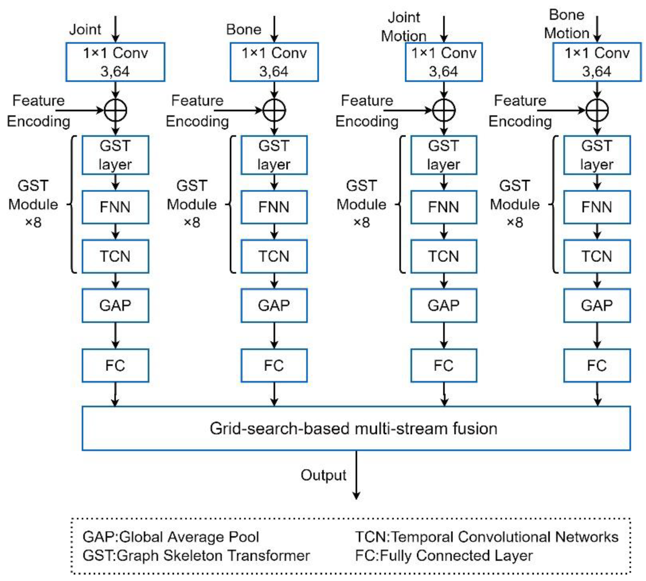
This section will address the relevant theory involved in our proposed approach, as shown in Figure 1. First, the network we proposed adopts the same four stream inputs as MS-AAGCN [24], which are: joint, bone, joint motion, and bone motion. The network of every stream is consistent. Second, for each stream input, the number of each channel is expanded from 3 to 64 by convolution. Third, feature encodings are added to each stream input. Fourth, the input passes through the graph transformer (GST) layer, feedforward neural network (FFN), and temporal convolution (TCN) in turn. We call the combination of the GST layer, FNN, and TCN the GST module, where each channel includes eight such modules. Fifth, the input passes through a global average pooling (GAP) and full connection layer (FC). Finally, all of the streams are fused into an output by the grid-search-based multi-stream fusion strategy.

In particular, in Section 3.1, the introduction of our methods starts with the positional and centrality encoding of the skeleton sequence, which is introduced to enhance the semantic and centrality information of the input. Then, in Section 3.2, the Graph Skeleton Transformer (GST) layer is introduced. To add natural information about the human body, the adjacency matrix information and the learnable mask matrix are fused based on the self-attention mechanism.

We introduce the GST module in Section 3.3 and the GST network composed of the GST module in Section 3.4. Finally, a multi-stream fusion strategy based on grid-search weights is presented in Section 3.5.

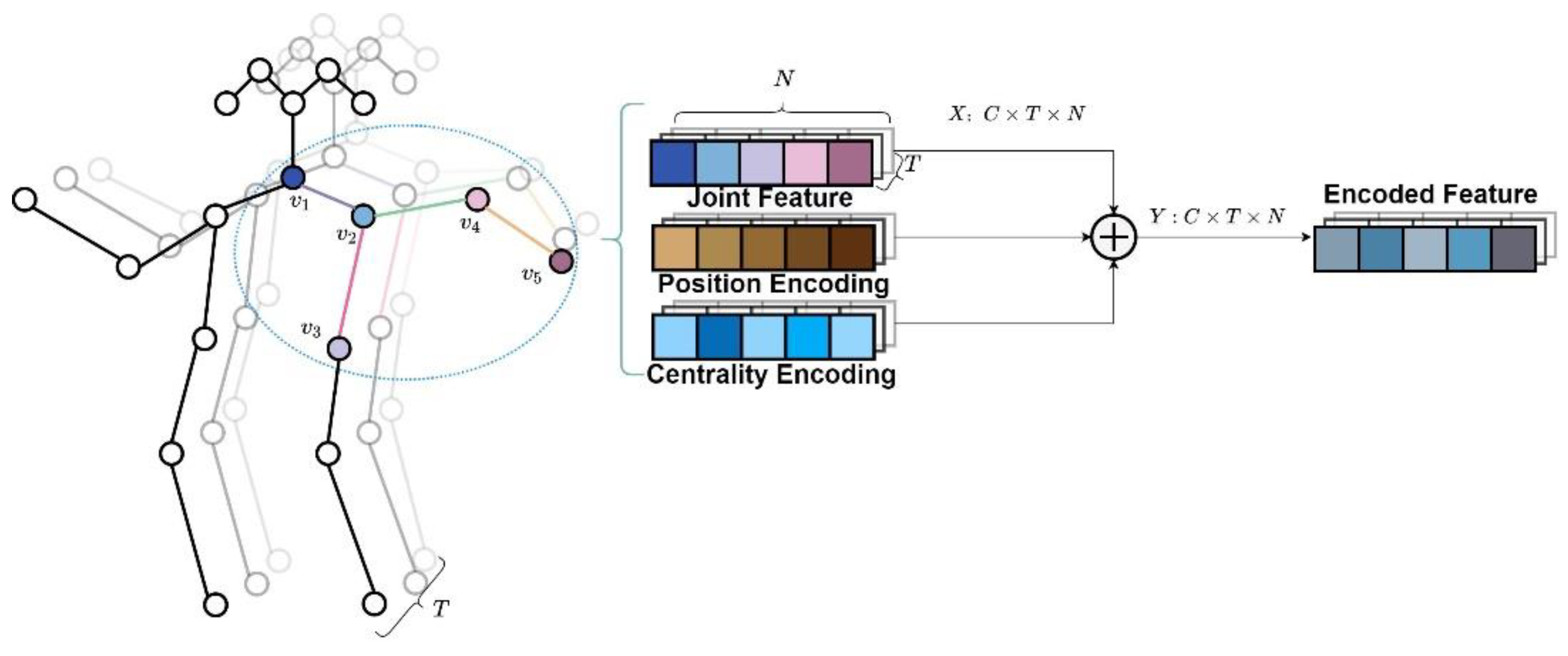
3.1. Feature Encoding

The input of the skeleton recognition task is a set of skeleton sequences containing both temporal and spatial dimensional information. We assume $X\in R^{N\times T\times C}$ is the input sequence for skeleton-based action recognition. $N$ denotes the number of key joints in the human skeleton, $C$ denotes the number of channels in the input sequence, usually the 3D coordinates of the skeleton, and $T$ denotes the number of frames in the sequence. The skeleton data is typically presented as an input in the form of a vector sequence in the same frame.

However, the input data are not encoded in the graph convolution-based method, resulting in features that lack semantic and centrality information in the input data. The existing Transformer-based methods encode the joint positions and do not consider the skeleton joints’ centrality. Experiments in Section 4.3.1 indicate that encoding data before input can improve model recognition while preserving the original data information. To ensure that the input sequence can fuse the semantic information and centrality information of joints, two types of encoding are applied: positional encoding and centrality encoding.

3.1.1. Spatial Position Encoding

In the field of natural language processing, positional encoding is a typical encoding method primarily used to rate the position of words in a sentence. However, in the skeleton-based action recognition task, positional encoding is done by numbering each joint according to its semantic class and embedding the number into the input features. In the work of other researchers, the joint position is not defined in advance for each skeleton joint, and in the input phase, a set of unordered tensors is fed into the network. The semantic features of the different joints in the model could not be represented.

For example, when the joint above the head is recognized as a hand or foot, the action category results of the recognition task are completely different. Since Vaswani et al. [26] demonstrated the effectiveness of the sine and cosine functions for positional encoding, we used a similar approach for the positional encoding of skeletal sequences, as shown in Equation (1):

$$\begin{array}{l}PE\left(p,2i\right)=sin\left(p/{10000}^{2i/C}\right)\hfill \\ PE\left(p,2i+1\right)=cos\left(p/{10000}^{2i/C}\right)\hfill \end{array}$$

(1)

where $p\in (1,2\cdots N)$ represents the skeleton joint category, $C$ represents the number of input channels, $2i$ represents the even-numbered item in the channel count, and $2i+1$ represents the odd-numbered item in the channel count.

$PE\left(p,2i\right)$ and $PE\left(p,2i+1\right)$ are conducted into a tensor $PE$ of the shape $N\times C$. Furthermore, at $t$ frame, the input $X_t\in R^{N\times C}$ has the same shape as $N\times C$, so that two tensors of the same shape can be added together. The position code is added to the input, as shown in Equation (2):

$$X_t=X_t+PE$$

(2)

where $X_t\in R^{N\times C}$ represents all the joint features of the $t$ frame, each frame’s joints would be encoded, so our joint features and the encoded shape are $C\times T\times N$, as shown in Figure 2.

3.1.2. Centrality Encoding

In graph structure, centrality is the main description of the importance of a joint. For example, in a skeleton graph, centrality indicates the number of skeletal edges that are connected to a joint. A joint at the end of a limb is adjacent to only one bone, whereas a joint in a central position can be adjacent to more than one bone. The joints with different centrality can influence action recognition differently. It is necessary to fuse information about the centrality of joints before input.

There are various ways to measure graph joint centrality, including closeness [31], betweenness, degree [32], etc. The degree of the human skeleton adjacency matrix can directly represent the centrality of the skeleton. In this paper, we use a centrality encoding method similar to Graphormer [33], which uses the degree information of the adjacency matrix as the centrality encoding.

We let the symmetric adjacency matrix constructed by the skeleton joints be $A\in R^{N\times N}$, and let $N$ be the number of body joints. A symmetric adjacency matrix is used to represent the undirected graph because the undirected graph can easily calculate the degree of each joint. The degree of the pth joint in the adjacency matrix, A, $d_p(A)$. The centrality is calculated as shown in Equation (3):

$$CE(p,A)=E_{d_p^{}(A)}^{}$$

(3)

where $E_{d_p^{}(A)}^{}$ is the embedding vector of the degree of the $p$th joint. The embedding dimension is equal to the number of channels $C$. Similarly, the centrality encode is added to the input, as shown in Equation (4), so that different centrality features for joints with different centralities are added:

$$X_t=X_t+CE$$

(4)

As shown in Figure 2, if all frames are position encoded and centrality encoded, the encoded features are shown in Equation (5):

$$Y_{}=X+PE+CE$$

(5)

where $Y$ is the encoded feature.

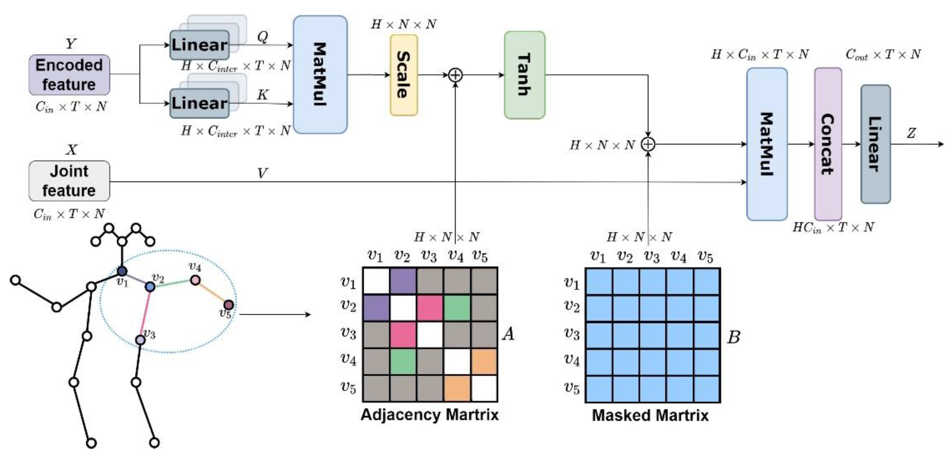
3.2. GST Layer

The GST layer is used to extract joint space information. A self-attention mechanism in the GST layer is introduced in Section 3.2.1. Section 3.2.2 discusses the method of introducing graph information into the self-attention mechanism. Section 3.2.3 introduces the multi-head attention mechanism.

The traditional visual Transformer network first transforms the input linearly to obtain $Q$, $K$, and $V$. $Q$ represents the query, $K$ represents the keyword, and $V$ represents the value. $Q$ is multiplied by $K$, and the result is normalized by scaling. Then, a Softmax function is introduced to obtain an attention map between 0 and 1. Then, the attention map is multiplied by $V$ to obtain the output, as shown in Equation (6):

$$\mathrm{Attention}(Q,K,V)=\mathrm{softmax}(\frac{Q{K}^T}{\sqrt{d_k}})V=(\mathrm{attmap})V$$

(6)

where $\sqrt{d_k}$ denotes scaling and $\mathrm{attmap}$ denotes the attention map.

3.2.1. Self-Attention Mechanism in the GST Layer

Referring to the traditional Transformer method [26], the paper encodes $X$ to get $Y$. $Y$ is linearly transformed to $Q$ and $K$, as shown in Equation (7). Finally, the original input is directly used as $V$:

$$Q=\varphi (Y),K=\phi (Y),V=X$$

(7)

where $\varphi$ and $\phi$ are trainable linear transforms, which only change the number of channels. Similar to the DSTA-net [8], in the skeleton recognition model, compared with the Softmax function, the tanh function can represent negative values. It is more flexible in expressing the attention map and can produce positive or negative attention. Therefore, we use tanh instead of Softmax, and the calculation formula of the attention map is shown in Equation (8):

$$\mathrm{attmap}=\tanh (\frac{Q{K}^T}{\sqrt{C}})$$

(8)

where $C$ is the number of channels of $Q$ or $K$.

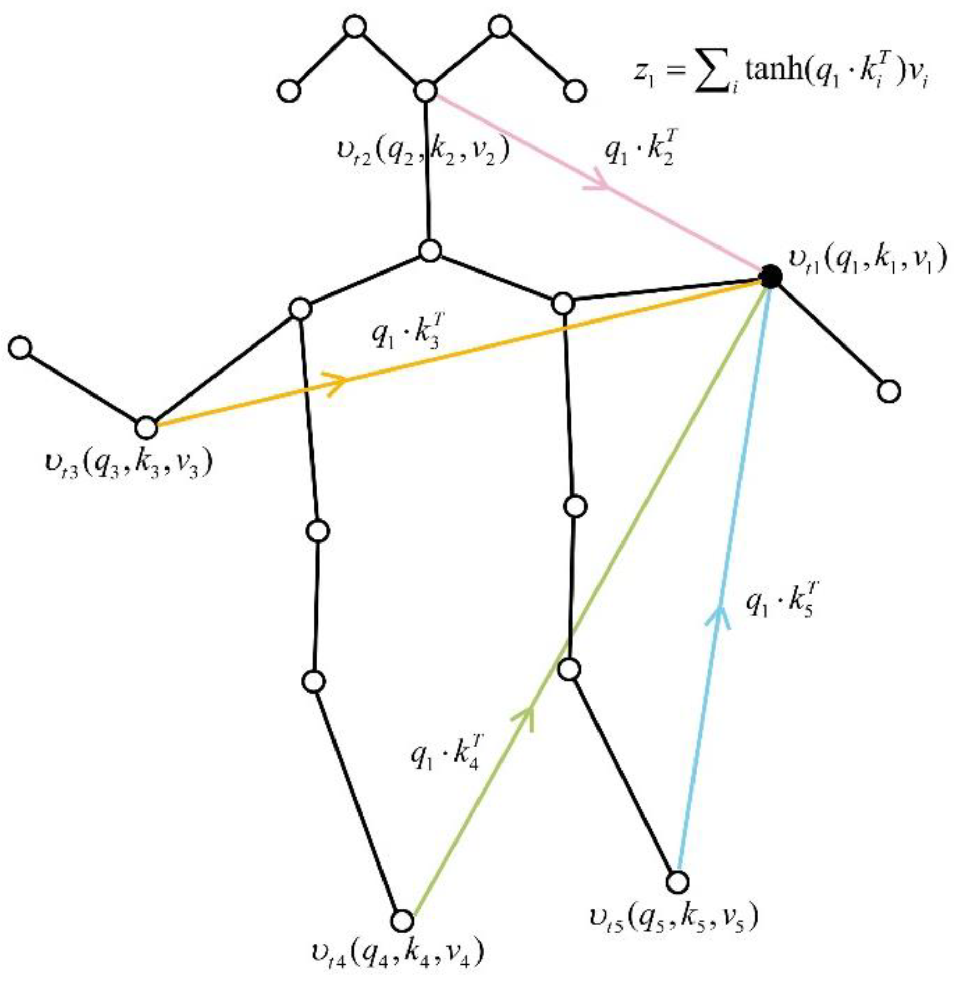
To analyze the attentional relationship between joint and other joints, we set $q$ and $k$ as elements in $Q$, $K$ respectively, representing a linear transformation of a joint in $Y$. The correlation information between the two joints is obtained by the dot product of $q$ and $k$. Let ${\upsilon }_i$ and ${\upsilon }_j$ be any two different joints, and ${\mathrm{z}}_{i,j}$ denote ${\upsilon }_i$ that updates the attention relation with ${\upsilon }_j$, as shown in Equation (9).

$${\mathrm{z}}_i={\displaystyle \sum _{j\in N}{\mathrm{z}}_{i,j}}={\displaystyle \sum _{j\in N(i)}(\tanh (\frac{q_i\cdot k_{{}_j}^T}{\sqrt{C}}))}{v}_j$$

(9)

where ${\mathrm{z}}_i$ indicates that the joint ${\upsilon }_i$ has updated its attention relationship with other joints, as shown in Figure 3.

3.2.2. Introduction of Graphical Information

The traditional Transformer approach does not focus on information about the graph structure. While in the graph structure, any two adjacent objects may have a data structure with a specific relationship. In the skeleton recognition task, the natural graph structure of the skeleton can better guide the model in learning local features. In recent years, there have been various related studies on Transformer incorporation of graph structure that have achieved results.

For example, ref. [34] modifies the original self-attention mechanism by adding a symmetric adjacency matrix, which performs well on various molecular prediction tasks, thereby extending the Transformer network to isomorphic graphs of arbitrary structure in [35]. The authors argue that to ensure graph sparsity, the attention mechanism in the Transformer should only aggregate information from neighborhoods (i.e., using the symmetric adjacency matrix as an attention mask). Furthermore, positional encoding is represented by the Laplacian eigenvectors, which naturally generalize the sinusoidal positional encodings often used in NLP. Their proposed model outperforms the baseline’s GNNs. The Graphormer proposed by Ying et al. [33] uses three encodings (centrality encoding, spatial encoding, and edge encoding) to fuse the information of the graph. The accuracy is improved compared to a traditional Transformer.

Inspired by the above research works and GCN-based methods [21,22,23,24,25], we believe that the undirect adjacency graph can express connectivity information of the human body, so the undirect adjacency graph information is added to the attention map. The experiment’s results in Section 4.3.2 verified the effectiveness of the graph information introduction. To represent an undirected graph, we design a symmetric adjacency matrix named $A\in R^{N\times N}$—as shown $N$ $a_{ij}$ is the number of body joints. The connectivity between joints named $a_{ij}$ is added to Equation (9), $a_{ij}$ represents the adjacency between ${\upsilon }_i$ and ${\upsilon }_j$ joints. The attention relationship between ${\upsilon }_i$ and other joints can be expressed as in Equation (10).

$${\mathrm{z}}_i={\displaystyle \sum _{j\in N(i)}(\tanh (\frac{q_i\cdot k_{{}_j}^T}{\sqrt{C}}+a_{ij}))v_j}$$

(10)

Considering all joints, the attention map is updated to Equation (11):

$$\mathrm{attmap}=\tanh (\frac{Q{K}^T}{\sqrt{C}}+A)$$

(11)

To make the model learn more attention, and to prevent overfitting of the model, we refer to the global regularization in DSTA-net [8], and a learnable attention mask matrix of the shape N × N is introduced to the attention map, which is called matrix $B$. As shown in Figure 4, matrix $B$ learns entirely from training data. The addition of this mask matrix allows the weights of the edges to be changed dynamically, and the attention map is further updated to Equation (12):

$$\mathrm{attmap}=\tanh (\frac{Q{K}^T}{\sqrt{C}}+A)+B$$

(12)

Finally, the original input feature $V$ is multiplied with the attention map, so that input $V$ gets the corresponding attention weight, as shown in Equation (13):

$$Z=(\mathrm{attmap})V=(\tanh (\frac{Q{K}^T}{\sqrt{C}}+A)+B)V$$

(13)

3.2.3. Multi-Head Attention

Most Transformer-based methods use multi-headed attention because multi-head attention allows the model to focus on features in different subspaces. We also adopt this method. As shown in Figure 4, we split the number of channels of input X into groups $H$ by using a linear transformation. $H$ is the number of heads of multi-head attention. The multi-head attention features can be expressed as ${\mathrm{z}}_i^1$, …, ${\mathrm{z}}_i^H$. Then, we connect the multi-head attention $Concat({\mathrm{z}}_i^1,\dots ,{\mathrm{z}}_i^H)$ to combine each head of the attention feature. The overall multi-headed attention can be expressed as Equation (14):

$$MHSA(Q,K,V)=Concat({\mathrm{Z}}^1,\dots ,{\mathrm{Z}}^H)$$

(14)

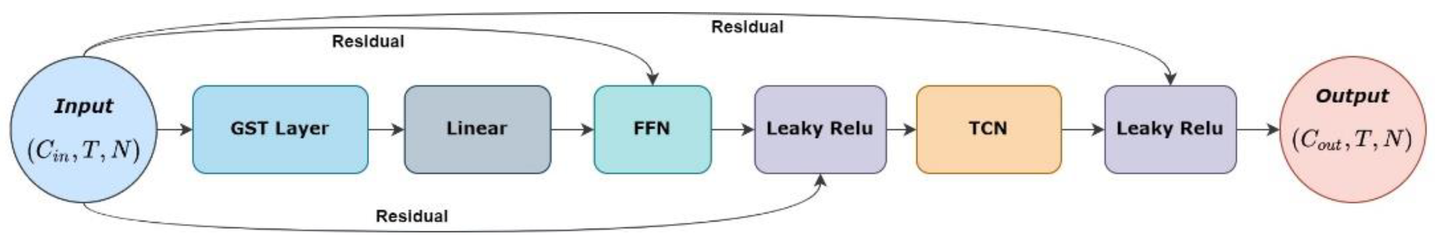
3.3. GST Module

The GST module extracts the spatial and temporal features of the input sequence, as shown in Figure 5. The GST module is composed of a GST layer, feedforward neural network layer (FFN), and temporal convolutional neural network layer (TCN). As described in Section 3.2, for the input $X\in R^{N\times T\times C}$, only spatial information is processed separately using the GST layer. We let the output after the GST layer extracts the information be represented as $Z\in R^{N\times T\times C}$. After the feedforward neural network, Z is input to TCN to extract the features of the skeleton sequence in the time dimension.

The convolution kernel of the feedforward neural network layer is 1 × 1, in order to realize the aggregation of output information. Its function is to process the characteristics of each joint independently and equally. Refs. [5,9] show that TCN can effectively extract the features of joint sequences in the temporal dimension. We use a 2D convolution, and the shape of the convolution kernel is (K, 1), where $Z\in R^{N\times T\times C}$ is the input of TCN, as shown in Equation (15):

$$Z_{}^{*}=f(W_K\otimes Z+\mathrm{B})$$

(15)

where $Z$ is the input to the TCN layer, $W_K$ is the K × 1 convolution kernel, $\otimes$ is the convolution, and $\mathrm{B}$ is the bias matrix. $f$ is the activation function, in this work, and the LeakyRelu activation function has been chosen. The output after TCN is $Z_{}^{*}$. To improve the stability of the training, three residual connections before and after the FFN layer, and after the TCN, are added.

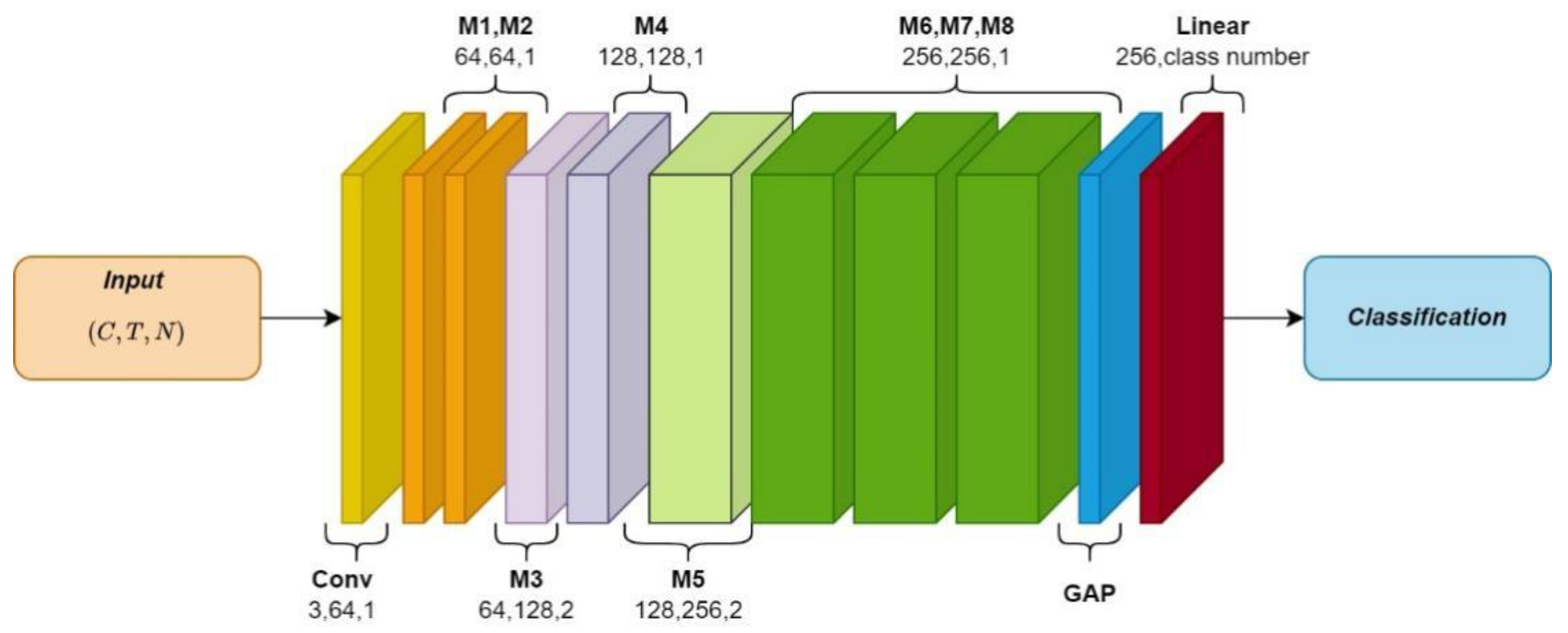
3.4. GST Network

The Graph Skeleton Transformer Network (GSTN) contains eight GST modules, as shown in Figure 6. M stands for GST module, and the output channels of the eight modules are 64, 64, 128, 128, 128, 256, 256, and 256, respectively.

The network takes the skeleton sequence ($N\times T\times C$) as an input. First, the convolution with a 1 × 1 kernel size is used, which expands the number of channels from 3 to 64. Then, the inputs pass through eight GST modules to extract the spatial–temporal features of the skeleton sequences. Then, we use the global average pooling layer to reduce the vector dimension to one dimension (only including the number of channels). Finally, a linear transformation of learnable parameters is adopted to map 256 channel data to the number of action categories.

3.5. Grid-Search-Based Multi-Stream Fusion Strategy

Some existing skeleton recognition methods [7,8,20,21,24] use multi-stream fusion strategies, resulting in significant accuracy improvements. In the process of building a multi-stream input network, most methods use manually fixed weight combinations and do not design a separate weight combination for each dataset setting. As described in [24], different input streams are complementary in different dataset settings. Therefore, it is necessary to set a multi-stream weight combination for each dataset. To avoid the extra time cost caused by manually finding the weight combination, and to find the optimal multi-stream weight combination more accurately, this paper proposes a multi-stream input strategy based on grid search.

The grid search method is an exhaustive search method for specified parameter values. It is also an ergodic parameter calling method. In this method, first, the possible values of each parameter are arranged and combined. Then, the results of all possible combinations are listed and a “grid” is generated. After traversing all parameter combinations, it is automatically adjusted to the best parameter combination.

In our experiments, a weight is assigned to each stream, where the range of weights was set to 0.3–0.7 and the step of variation is 0.1. We traverse all the weight combinations in this interval and output the accuracy. By comparing the accuracy, we can find the weight combination with the highest accuracy.

4. Experiments

We used three human action recognition datasets (NTU RGB+D 60 [36], NTU RGB+D 120 [37], and NW-UCLA [38]). The specific contents of the three ablation experiments are as follows: First, we did ablation experiments on the NW-UCLA dataset to demonstrate the effectiveness of the two types of encoding. Secondly, we tested the validity of two matrices (the adjacency matrix $A$ and the learnable mask matrix $B$) that were added to the attention map on the NTU RGB+D 60 dataset. Then, to test the effectiveness of the grid-search-based multi-stream fusion strategies, we recorded the best weight combination searched by each benchmark of each dataset. Finally, we compared the accuracy of the above optimal combination with that of multi-stream fusion with fixed weights. At last, we compared the experimental results with state-of-the-art methods.

4.1. Datasets

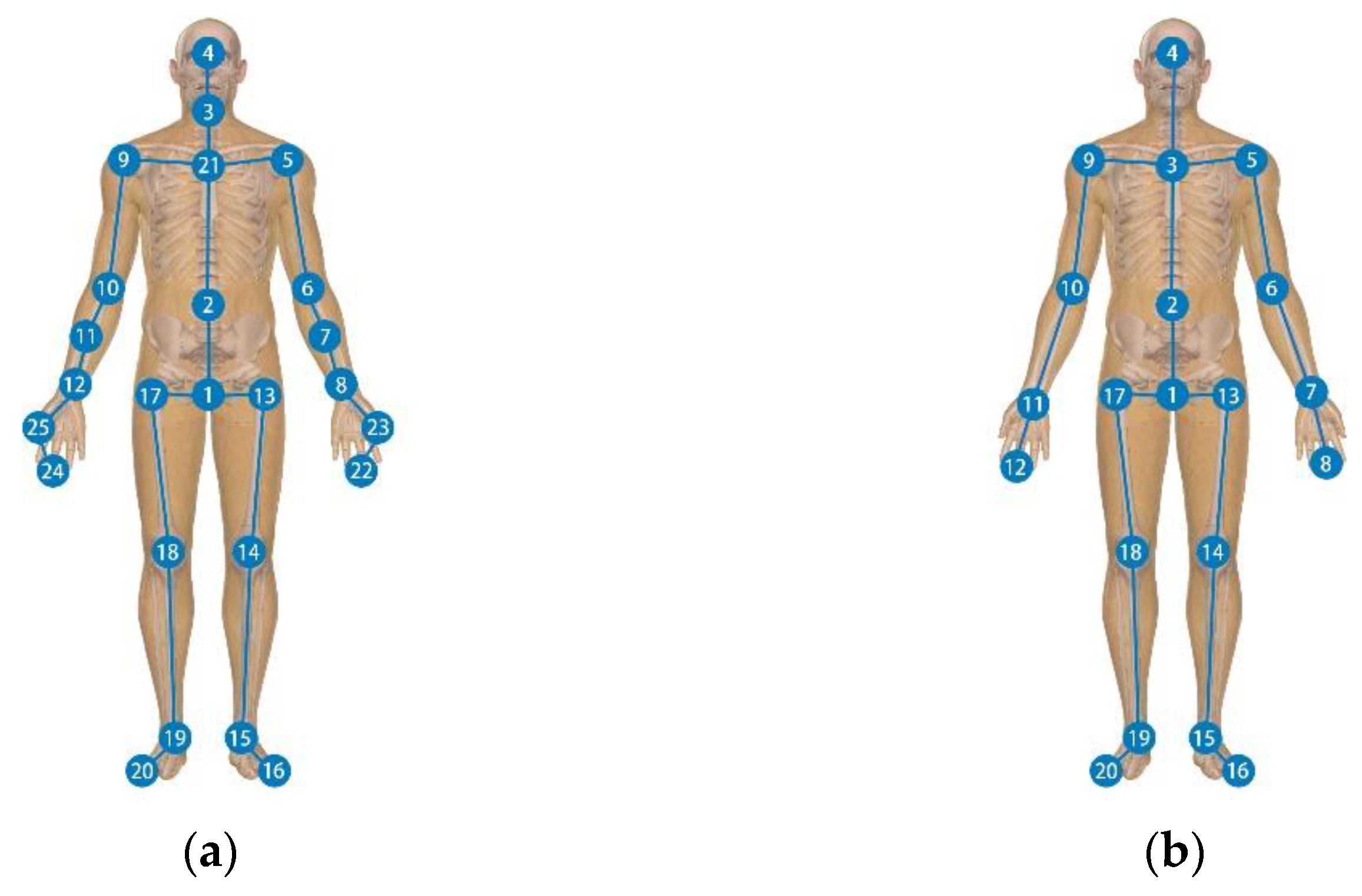
NTU RGB+D 60: The NTU RGB+D 60 dataset [36] is a widespread human action recognition dataset containing 56,000 action clips and 4 million frames. These clips were captured by 40 subjects in a filming laboratory environment using three different views of Kinect v2 [39]. Every subject contains 25 joint points and their 3D positions, as shown in Figure 7. In addition, 60 action categories are available in the NTU RGB+D dataset, the last 11 of which are double people actions. The evaluation benchmarks for this dataset include cross-subject (X-Sub) and cross-view (X-View). The training and test sets consisted of 40,320 and 16,560 video clips. In the cross-subject benchmark, the training clips were taken from a subset of the subjects, and the test clips were taken from the remaining subjects. The training and test sets in the X-View benchmark consisted of 37,920 and 18,960 clips, respectively. The 37,920 clips captured from cameras 2 and 3 were used for training and the other 18,960 clips captured from camera 1 were used for testing.

NTU RGB+D 120: The NTU RGB+D 120 dataset [37] extends the NTU RGB+D 60 dataset and is currently the largest dataset containing 3D joint information. It includes 57,600 new action clips to represent 60 new action categories, a total of 114,480 video clips, and 120 action categories for a total of 106 subjects, which were filmed from 32 different camera settings. The dataset also followed two benchmark assessments: cross-subject (X-Sub) and cross-setup (X-Set). In the X-Sub benchmark research, similar to NTU RGB+D 60, the 106 subjects were divided into a training and a test group, each containing 53 subjects. For the cross-view evaluation, the 32 camera setup IDs were split into two parts according to the serial number of the IDs, with the even-view IDs being used for training and the odd-view IDs for testing.

NW-UCLA: The NW-UCLA is known as the Northwestern–UCLA dataset [38]. It is also captured by three Kinect cameras. It contains 1494 clips covering 10 action categories. Each action is performed by 10 actors. The evaluation protocol is the same as in [38]. Samples from the first two cameras constitute the training data and samples from the other camera constitute the testing data.

The position of each joint in the NTU RGB+D 60 datasets and the NW-UCLA datasets is shown in Figure 7.

4.2. Experimental Details

All experiments were performed in the PyTorch framework and were optimized using a stochastic gradient descent method with Nesterov momentum (0.9). A GeForce NVIDIA 3090 GPU was used for training. We used a cross-entropy loss function. To prevent overfitting of the model, we used L2 regularization, and the weight decay is set to 0.0005.

For the NTU RGB+D 60 and NTU RGB+D 120 datasets, the partitioning and pre-processing were done using the 2s-AGCN method. The maximum number of training epochs is set to 60, and the batch size is 64. A strategy that updates the learning rate with the number of training steps is introduced. The initial learning rate is 0.1. At 20 and 40 steps, the learning rate is multiplied by 0.1.

The partitioning of the NW-UCLA dataset is done according to the cross-view setting in [38]. The initial learning rate is 0.1. The maximum number of training epochs is 200. The learning rate is updated as the accuracy increases. The batch size is set to 16, and the learning patience is set to 12. The learning threshold is set to 0.0001.

In Section 4.3.3, the performance of a grid-search weight method for the multi-stream fusion strategy is compared with conventional multi-stream fusion strategies. The multi-stream inputs are the same as [24], including joint (J), bone (B), joint motion (JM), and bone motion (BM).

4.3. Experimental Details

4.3.1. Effectiveness of Feature Encoding

To verify the effectiveness of feature encoding, we listed the accuracy of using the centrality encoding (CE) and position encoding (PE) in

Table 1. The effectiveness of centrality encoding and position encoding on the NW-UCLA dataset. Fusion denotes the fusion of the four streams.

Encoding Method		Acc (%) (J)	Acc (%) (B)	Acc (%) (JM)	Acc (%) (BM)	Acc (%) (Fusion)
CE	PE
✗	✗	92.5	89.01	90.1	87.7	94.8
✓	✗	90.9	92.0	91.2	88.1	95.5
✗	✓	92.2	92.7	92.2	88.1	95.0
✓	✓	92.5	93.8	90.3	88.1	95.9

. Our experiments were set up to use no encoding, only use CE, only use PE, and both CE and PE.

As shown in Table 1, CE + PE in the joint stream achieved the highest result of 92.5%, and in the bone stream, CE + PE achieved the highest accuracy of 93.8%, which is at least 1% ahead of the other encoding methods. In the JM stream, the highest accuracy was achieved using PE alone, while in the BM stream, there was little difference between the various encoding methods, and in the final four-stream fusion, the highest accuracy was achieved using both encodings. The experimental results show that both centric and positional encoding help to improve recognition accuracy. The effect is enhanced even more when the two methods are combined, which also demonstrates the necessity of adding semantic information to skeleton joints.

4.3.2. Effectiveness of the Introduction of Graphical Information

To verify the effectiveness of our introduction of graph information in the Transformer, we conducted separate ablation experiments for the added adjacency matrix $A$ and the learnable mask matrix B. The comparative analysis shows that adding the adjacency matrix alone, without the learnable mask matrix, results in a lossy non-convergence of the model. Therefore,

Table 2. The effectiveness of graph information introduction on the X-Sub benchmark of NTU RGB+D 60 dataset.

Matrix		Acc (%) (J)	Acc (%) (B)	Acc (%) (JM)	Acc (%) (BM)	Acc (%) (Fusion)
A	B
✗	✗	86.0	86.3	84.1	83.6	90.6
✗	✓	87.4	86.9	85.0	85.5	90.6
✓	✓	87.6	87.9	85.7	85.7	91.3

shows the comparison results using the matrix, the matrix $A$ + $B$, and not using any matrix.

The experimental results show that adding matrix $B$ alone improves the accuracy by 0.3%. Adding both matrix A and matrix B at the same time improves the accuracy significantly after the fusion of multiple streams, although the improvement in accuracy is not high for every single stream using the adjacency matrix. We believe that the two added matrices have complementary contributions to different motion recognition in the four inputs. This is because more abundant information can be extracted by adding two kinds of matrices to introduce graph information.

4.3.3. Effectiveness of Grid-Search-Based Multi-Stream Fusion Strategy

Table 3. The detailed accuracy (%) of the multi-stream inputs in the NTU RGB+D 60 dataset.

Methods	X-Sub	X-View
J-GSTN	87.6	95.1
B-GSTN	87.9	93.5
JM-GSTN	85.7	92.9
BM-GSTN	85.7	92.8
2s-GSTN	89.8	95.7
4s-GSTN	91.3	96.6

shows the details of the multi-stream inputs in the NTU RGB+D 60 dataset. The 2s denote the joint stream and bone stream. The 4s denote all 4 streams. The results show that the accuracy has improved significantly with the two-stream inputs and reaches even higher accuracy with the fusion of the four-stream inputs.

To demonstrate the validity of grid-search weights for multi-stream fusion strategies, we used multi-stream fusion with fixed weights as a comparison. We have designed a weight that can be automatically searched for each class of four stream inputs. The weight range of each stream is 0.3–0.7. The step is 0.1. The highest precision weights are obtained after the grid-search traversal of all weight combinations. The highest accuracy and corresponding weights are recorded in

Table 4. The effectiveness of the multi-stream fusion strategy with or without grid-search. NTU60 denotes the NTU RGB+D 60 dataset, and NTU120 denotes the NTU RGB+D 120 dataset.

Datasets	Weight (J)	Weight (B)	Weight (JM)	Weight (BM)	Acc (%) (Fusion W/O GS)	Acc (%) (Fusion w/GS)
NTU60 X-Sub	0.6	0.6	0.4	0.5	91.1	91.3
NTU60 X-View	0.5	0.5	0.4	0.4	96.5	96.6
NTU120 X-Sub	0.5	0.7	0.4	0.3	86.0	86.3
NTU120 X-Set	0.4	0.6	0.4	0.3	88.4	88.7
NW-UCLA	0.4	0.6	0.6	0.4	95.7	95.9

.

Table 4 shows the weights of each stream by grid search and the fusion results. Fusion w/o GS indicates a configuration where the weights of each stream are all fixed to 1. Fusion w/GS shows the results of multi-stream fusion after using the grid search. As can be seen from the table, the weights obtained by applying the automatic weight search are 0.1–0.3% more accurate than when fusing the four-stream directly.

4.4. Comparison with Previous Methods

We evaluated our method with state-of-the-art methods for skeleton-based action recognition on three datasets: NTU RGB+D 60, NTU RGB+D 120, and NW-UCLA.

As shown in

Table 5. Comparisons of the accuracy (%) with the state-of-the-art methods on the X-Sub and the X-View benchmark of the NTU RGB+D 60 dataset.

Methods	Year	X-Sub	X-View
Lie Group [11]	2014	50.1	52.8
VA-LSTM [15]	2017	79.4	87.6
TCN [42]	2017	74.3	83.1
Synthesized CNN [19]	2017	80.0	87.2
2s-AGCN [9]	2019	88.5	95.1
SGN [22]	2020	89.0	94.5
4s-Shift-GCN [21]	2020	90.7	96.5
PA-ResGCN-B19 [40]	2020	90.9	96.0
TRIPOOL [41]	2021	88.0	95.3
ST-TR [29]	2021	89.9	96.1
DSTA-net [8]	2021	91.5	96.4
KA-AGTN [30]	2022	90.4	96.1
MTT [43]	2022	90.8	96.7
4s-GSTN (ours)	-	91.3	96.6

, our model has an excellent performance in the NTU RGB+D 60 datasets. “VA-LSTM” [15] and “Synthesized CNN” [19] are two representative methods for RNN-based and CNN-based methods, respectively. GSTN outperforms them by 11.9% and 11.3% in accuracy for the X-Sub benchmark, respectively. Compared with GCN-based methods [9,21,22,40,41], our method has higher accuracy than the above methods. In contrast to the latest method, KA-AGCN [30], which applies Transformer and GCN, our model does not use GCN but adds the topological structure of the graph to the attentional map. Our method outperforms the KA-AGCN by 0.9% on the X-Sub benchmark and 0.5% on the X-Set benchmark.

Compared with the state-of-the-art methods on NTU RGB+D 120, our method has higher accuracy than the GCN-based methods [21,22,40,41] and GCN combined with Transformer methods [29,30,43], as is shown in

Table 6. Comparisons of the accuracy (%) with the state-of-the-art methods on the X-Sub and X-Set benchmark of the NTU RGB+D 120 dataset.

Methods	Year	X-Sub	X-Set
SGN [22]	2020	79.2	81.5
4s-Shift-GCN [21]	2020	85.9	87.6
PA-ResGCN-B19 [40]	2020	87.3	88.3
TRIPOOL [41]	2021	80.1	82.8
ST-TR [29]	2021	82.7	84.7
KA-AGTN [30]	2022	86.1	88.0
MTT [43]	2022	86.1	87.6
4s-GSTN (ours)	-	86.4	88.7

. In addition, our method outperforms the KA-AGTN by 0.3% on the X-Sub benchmark and 0.7% on the X-Set benchmark.

As shown in

Table 7. Comparisons of the accuracy (%) with the state-of-the-art methods on the NW-UCLA dataset.

Methods	Top-1
Lie GROUP [11]	74.1
Actionlet ensemble [18]	76.0
HBRNN-L [44]	78.5
Ensemble TS-LSTM [45]	89.2
2s-AGC-LSTM [46]	93.3
4s-Shift-GCN [21]	94.6
4s-GSTN (ours)	95.9

, our model achieves state-of-the-art performance in the NW-UCLA dataset, and 1.3% higher accuracy than Shift-GCN [21]. Compared with manual feature extraction [11], CNN-based methods [18], and RNN-based methods [44,45,46], our method has much higher accuracy.

To verify the training speed of the Transformer network, we compared our method with a traditional graph convolutional network-2s-AGCN, and we compared it with two lightweight networks, as shown in

Table 8. Comparisons of the run time performance with the traditional methods and the faster methods on the NTU RGB+D 60 dataset.

Method	Params	GFlops	Speed (ms)
AGCN [9]	3.47	9.34	75.2
SGN [22]	0.69	3.4	15.2
ResGCN-n51 [40]	0.77	-	16.8
1s-GSTN (ours)	3.80	7.91	15.6

. We used an Intel (R) Xeon(R) Silver 4210R CPU (2.40 GHz) and a GeForce NVIDIA 3090 GPU, and we tested the 16,487 sequences in the NTU RGB+D 60 dataset and calculated the average time to predict an action sequence, denoted as speed. As a result, our model’s computation time with a single stream input was nearly 0.2 times that of AGCN, which is comparable to the faster models of SGN and ResGCN-n51.

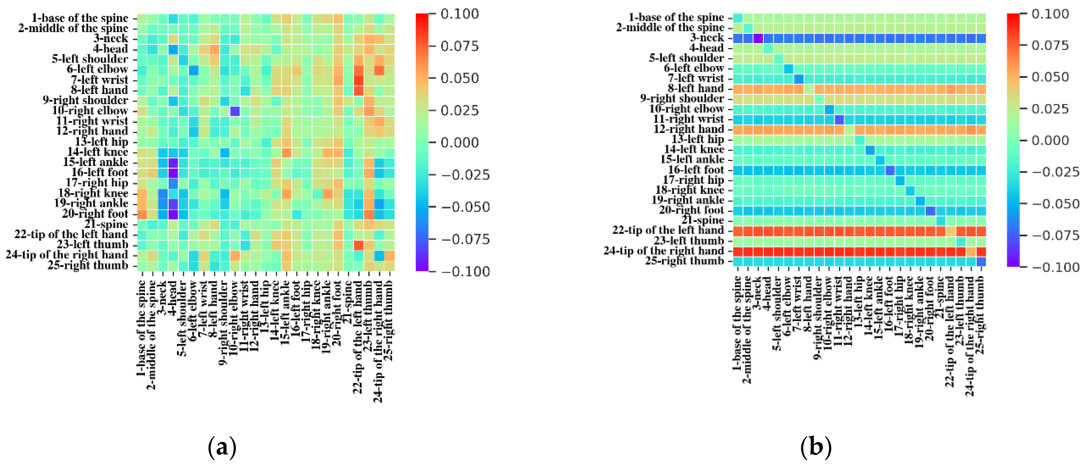
4.5. Visualization of Attention Map

Since our model is based on a self-attention mechanism, the attention map was visualized to demonstrate the effectiveness of our self-attention mechanism. As shown in Figure 8: (a) shows the attention map of the first GST layer of our model, and (b) shows the attention map of the last GST layer of our model.

The attention maps learned in each layer are different because the semantic information contained in each layer is not the same. In addition, the attention in the first layer map is more focused on parts related to the limbs (ankles, feet, hands, fingers, etc.). The focus on the head is less pronounced. This phenomenon is due to the joints in the limbs having an inherent ability to distinguish between human actions. When information is highly aggregated at a higher level, the differences between each joint become less obvious, and thus the phenomenon becomes less obvious.

5. Conclusions

In this work, we propose a Graph Skeleton Transformer Network (GSTN) for action recognition. The main contributions of the paper include: (1) The skeleton joints have been encoded so that the joints’ features contain information about the position and centrality. (2) Graph information is added to make up for the lack of graph information in the Transformer. (3) Grid-search was used in the multi-stream fusion strategies, and these methods outperformed previous methods in terms of recognition accuracy. Advanced results were achieved on three major datasets. Finally, we tested the model’s speed. The results show that the Transformer-based method is more than five times faster than the traditional 2s-AGCN method.

In the field of skeleton-based action recognition, due to the adoption of the multi-stream fusion strategy, the number of calculations and parameters are large. It lacks application in portable embedded systems. In the time dimension, the traditional TCN is still used, which brings large parameters and FLOPs. After we tried shift convolution and dilated convolution methods, the accuracy decreased, thus we adopted the traditional TCN method.

Scope of future work should aim to fuse the multi-stream before inputting the model, and to use the time transformer in the time dimension to replace the convolution operation. All of the above aim to further reduce the parameters and FLOPs and improve recognition accuracy.