Fractional-View Analysis of Fokker-Planck Equations by ZZ Transform with Mittag-Leffler Kernel

Abstract

This work combines a ZZ transformation with the Adomian decomposition method to solve the fractional-order Fokker-Planck equations. The fractional derivative is represented in the Atangana-Baleanu derivative. It is looked at with graphs that show that the accurate and estimated results are close to each other, indicating that the method works. Fractional-order solutions are the most in line with the dynamics of the targeted problems, and they provide an endless number of options for an optimal mathematical model solution for a particular physical phenomenon. This analytical approach produces a series type result that quickly converges to actual answers. The acquired outcomes suggest that the novel analytical solution method is simple to use and very successful at assessing complicated equations that occur in related research and engineering fields.

1. Introduction

Fractional calculus (FC) depicts the facts of existence in a more straightforward manner. Making this issue accessible to the world of engineering and science as a common topic offers another layer for better understanding or expressing fundamental natures. Because FC is the language that nature knows, connecting with it in this manner is effective. This issue of FC has been with mathematicians over the previous three centuries, and it has just recently been pulled into other practical sectors of engineering, science, and economics [1,2,3,4,5,6]. FC deals with integrals and derivatives in any real or complex order. Atangana-Baleanu, Caputo, Caputo Fabrizio, Hilfer, Katugampola, and other fractional operators have recently been suggested and implemented to cope with real-world applications. In this paper, we looked at a non-singular and non-local fractional operator using the Mittag-Leffler function as its kernel, which may be used to mimic a variety of real-world issues. Due to its non-singularity and non-locality, it has been termed the Atangana-Baleanu fractional operator, and there are a number of illustrative uses in the literature [7,8,9,10,11]. Several major strategies have been utilised, such as the fractional operational matrix technique [12], Shehu decomposition technique [13,14], q-homotopy transformation method [15], homotopy perturbation method [16,17], and variational iteration transform technique [18]. The foundation of nature is symmetry, however the great majority of natural occurrences lack symmetry. In order to conceal symmetry, it is effective to break unexpected symmetry. There are two kinds of symmetry: finite and infinitesimal. There can be discrete or continuous symmetries in finite symmetries. Natural symmetries include symmetry and time reversal are discontinuous, whereas space is a constant transformation. Mathematicians have been fascinated by patterns for millennia. The eighteenth century witnessed the emergence of systematic categorization of planar and spatial patterns.

The link between the Aboodh transformation (AT), the ZZ transformation (ZZT), and the Laplace transformation (LT) is established in this study, with numerous applications described in [19,20,21]. Later, we used this ZZ transform to solve various test examples described in the Atangana-Baleanu sense. The current author’s contributions to this work are first establishing the link among the Laplace, Aboodh, and ZZ transformations, and second, using the ZZ transform to solve fractional differential equations expressed in the Atangana-Baleanu derivative. The ZZ transform generalizes a few well-known transforms, which can be related to other well-known ones. The Natural transform is obtained by dividing the ZZ transform by the modified variable. This work also includes relationships with other integral transformations in terms of theorems. This transformation has the virtue of converging to the Sumudu transformation, which is useful when solving fractional differential equations with variable coefficients [22,23,24]. Adomian (1980) established the Adomian decomposition technique (ADM), an efficient method for finding explicit and numerical solutions to a larger and more general class of differential systems representing real-world issues [25,26,27]. This strategy effectively addresses initial and boundary value problems, linear and nonlinear, ordinary and partial differential equations, and stochastic systems. Furthermore, this approach does not require any linearization or perturbation. ADM has been used extensively in the last two decades, since it yields approximate analytical solutions for nonlinear problems, and there has been much interest in utilizing it to solve fractional differential equations [28,29,30].

The Fokker-Planck equation was mainly implemented by Fokker and Planck to recognize the Brownian suggestion of particles. It is notable that the fractional order Fokker-Planck (FP) equations are a mathematical concept used in both the biological and physical sciences. The spread of its Markovian and continuous character leads to the approximation of some randomizations, in acceptable processes and procedures [31]. The Fokker-Planck equations are used in various applied sciences, such as electron relaxation, polymer dynamics, quantum optics, solid-state system and probability flux [32].

Consider the fractional-order FP equation in the general form, as:

$${}^{ABC}{\nu }_{\rho }^{\gamma }(\phi ,\rho )={\nu }_{\phi }(\phi ,\rho )+{\nu }_{\phi \phi }(\phi ,\rho ),\phi \in R\rho >0,\gamma \in (0,1],$$

(1)

with the initial condition:

$$\nu (\phi ,0)=\zeta \left(\phi \right).$$

The fractional-order Fokker-Planck equations have been successfully implemented in different areas, such as chemical physics, biological molecules, engineering, and energy consumption. In fact, fractional diffusion, a specific type of fractional-order Fokker-Planck equation, has also been applied in a wide range of situations, including diffusion processes, viscoelasticity, and frequency-dependent material damping behavior [31]. However, it is difficult to analysis a precise solution for fractional problems. Several analytical and numerical techniques applied for fractional-order Fokker-Planck equations include the Laplace transformation technique [32], the multi-step reduced differential transformation technique [33], the predictor corrector method [34], the Adomain decomposition technique [35], and the variational iteration technique [36].

Here, papers [37,38,39,40,41] address the application of ADM to various transport models, also including fractional and nonlinear cases; works [42,43,44,45,46] provide reviews or/and developments of various computational approaches to linear [43,44,45,46] and nonlinear [42,43,45] transport/advection-diffusion problems; [47] introduces a homotopy perturbation method for nonlinear transport equations, while [48] proposes perturbational approach to construct analytical approximations based on the double-parameter transformation perturbation expansion method. Finally, the review paper [49] contains an exhaustive review of various modern fractional calculus applications, and paper [50] discusses some non-standard definitions of Caputo fractional derivatives, while paper [51] provides a comprehensive overview of computational practices used in fractional calculus. In this study, we utilized the Modified decomposition method (MDM) to solve fractional-order Fokker-Planck equations. The Adomian decomposition technique [52,53] is a very good technique for solving linear and non-linear partial differential equations, as well as integral differential and fractional differential equations, in a series type solution. The obtained solutions to the fractional problems applying the suggested technique are also utilized the analysis of the equations. It has been proven that the suggested method can be used to analyze a variety of fractional partial differential equations and systems.

2. Preliminaries

Definition 1.

An Aboodh transformation (AT) is given for terms of exponential order. We consider term in the set B, expressed by:

$$B=\left\{h:\left|h\left(\rho \right)\right|<M{e}^{n_j\left|\rho \right|},\mathrm{if}\rho \in {(-1)}^j\times [0,\infty ),j=1,2;\left(M,n_1,n_2>0\right)\right\}.$$

M must be a finite number for a given function in set B; $n_1,n_2$ may be finite or infinite.

Then, the AT denote by the operator $A(.)$ is expressed as the integral equation [19,20]:

$$A\left\{h\left(\rho \right)\right\}=\frac{1}{\varsigma }{\int }_0^{\infty }h\left(\rho \right)e^{-\varsigma \rho }d\rho ,\rho \ge 0,n_1\le \varsigma \le n_2.$$

Theorem 1.

Now, we consider G and F as the Laplace and Aboodh transformations of $h\left(\rho \right)\in B$, then [21,22]:

$$G\left(\varsigma \right)=\frac{F\left(\varsigma \right)}{\varsigma }.$$

Zain U. Zafar [23] was the first to develop the ZZ transform. It is a mixture of the Laplace transform and AT. The ZZ transformation is expressed.

Definition 2.

(ZZ transform) Suppose that $h\left(\rho \right)\forall \rho \ge 0$ is a function, then the ZZ transformation $\mathcal{Z}(\varrho ,\varsigma )$ of $h\left(\rho \right)$ is defined as [23]:

$$\mathcal{Z}\left(h\left(\rho \right)\right)=\mathcal{Z}(\varrho ,\varsigma )=\varsigma {\int }_0^{\infty }h\left(\varrho \rho \right)e^{-\varsigma \rho }d\rho .$$

The ZZ transformation is linear, as are the Aboodh and Laplace transforms. The Mittag-Leffler function is given as

$$E_{\delta }\left(z\right)=\sum _{ȷ=0}^{\infty }\frac{z^{ȷ}}{\Gamma (1+ȷ\delta )},Re\left(\delta \right)>0.$$

Definition 3.

The Atangana-Baleanu derivative (ABD) of a term $\nu (\phi ,\rho )\in H^1(a,b)$, then for $\delta \in$$(0,1)$, is defined as [24]:

$${}_a^{ABC}{D}_{\rho }^{\delta }\nu (\phi ,\rho )=\frac{\psi \left(\delta \right)}{1-\delta }{\int }_a^{\rho }{\nu }^{\prime }(\phi ,\rho )E_{\delta }\left(\frac{-\delta {(\rho -\eta )}^{\delta }}{1-\delta }\right)d\eta .$$

Definition 4.

Let $\nu (\phi ,\rho )\in H^1(a,b)$, then for $\delta \in (0,1)$, the Riemann-Liouville ABD is defined as [24]:

$${}_a^{ABR}{D}_{\rho }^{\delta }\nu (\phi ,\eta )=\frac{\psi \left(\delta \right)}{1-\delta }\frac{d}{d\rho }{\int }_a^{\rho }\nu (\phi ,\eta )E_{\delta }\left(\frac{-\delta {(\rho -\eta )}^{\delta }}{1-\delta }\right)d\eta ,$$

with the condition $\psi \left(0\right)=\psi \left(1\right)=1$, $\psi \left(\delta \right)$ is a normalization function, and $b>a$.

Theorem 2.

The Laplace transform of the Riemann-Liouville Atangana-Baleanu derivative is expressed as [24]:

$$\mathrm{L}\left\{{}_a^{ABC}{D}_{\rho }^{\delta }\nu (\phi ,\rho )\right\}\left(\varsigma \right)=\frac{\psi \left(\delta \right)}{1-\delta }\frac{{\varsigma }^{\delta }L\left\{\nu (\phi ,\rho )\right\}-{\varsigma }^{\delta -1}\nu (\phi ,0)}{{\varsigma }^{\delta }+\frac{\delta }{1-\delta }}$$

and

$$L\left\{\begin{array}{c}ABR\hfill \\ a\hfill \end{array}{D}_{\rho }^{\delta }\nu (\phi ,\rho )\right\}\left(\varsigma \right)=\frac{\psi \left(\delta \right)}{1-\delta }\frac{{\varsigma }^{\delta }L\left\{\nu (\phi ,\rho )\right\}}{{\varsigma }^{\delta }+\frac{\delta }{1-\delta }}$$

The theorems that follow are based on the idea that $h\left(\rho \right)\in H^1(a,b),b>a$ and $\delta \in (0,1)$.

3. Methodology of MDM

The general implementation of the given method

$${}^{ABC}{D}_{\rho }^{\delta }\nu (\phi ,\rho )=\overline{\mathcal{H}}(\phi ,\rho )+\mathcal{N}(\phi ,\rho ),0<\delta \le 1,$$

(2)

with the initial condition:

$$\nu (\phi ,0)=\xi \left(\phi \right),$$

where ${}^{ABC}{D}_{\rho }^{\delta }$ is the Atangana-Baleanu fractional derivative of order $\delta$; $\overline{\mathcal{H}}$ is a linear and $\mathcal{N}$ a nonlinear term.

On both sides, using the ZZ transformation of Equation (2), to achieve:

$$\mathcal{Z}\left[\nu (\phi ,\rho )\right]=\mathcal{Z}[\overline{\mathcal{H}}(\phi ,\rho )+\mathcal{N}(\phi ,\rho )].$$

(3)

By the differentiation property of the ZZ transformation, we get:

$$\frac{\psi \left(\delta \right)}{\left(1-\delta +\delta {\left(\frac{\varrho }{\varsigma }\right)}^{\delta }\right)}\mathcal{Z}\{\nu (\phi ,\rho )-\frac{\varrho }{\varsigma }\nu (\phi ,0)\}=\mathcal{Z}[\overline{\mathcal{H}}(\phi ,\rho )+\mathcal{N}(\phi ,\rho )].$$

(4)

Equation (4) implies that:

$$\mathcal{Z}\left(\nu (\phi ,\rho )\right)=\frac{\varrho }{\varsigma }\nu (\phi ,0)+\frac{\left(1-\delta +\delta {\left(\frac{\varrho }{\varsigma }\right)}^{\delta }\right)}{\psi \left(\delta \right)}\mathcal{Z}[\overline{\mathcal{H}}(\phi ,\rho )+\mathcal{N}(\phi ,\rho )],$$

(5)

Applying the ZZ inverse transformation of Equation (5), we get:

$$\nu (\phi ,\rho )=\nu (\phi ,0)+{\mathcal{Z}}^{-1}[\frac{\left(1-\delta +\delta {\left(\frac{\varrho }{\varsigma }\right)}^{\delta }\right)}{\psi \left(\delta \right)}\mathcal{Z}\left\{\overline{\mathcal{H}}(\phi ,\rho )+\mathcal{N}(\phi ,\rho )\right\}].$$

(6)

MDM determines the infinite sequence’s result of $\nu (\phi ,\rho )$:

$$\nu (\phi ,\rho )=\sum _{ȷ=0}^{\infty }{\nu }_{ȷ}(\phi ,\rho ).$$

(7)

The non-linear functions $\mathcal{N}$ is expressed as:

$$\mathcal{N}(\phi ,\rho )=\sum _{ȷ=0}^{\infty }{\mathcal{A}}_{ȷ}.$$

(8)

The Adomian polynomials can show all types of non-linear functions, as:

$${\mathcal{A}}_{ȷ}=\frac{1}{ȷ!}{\left[\frac{{\partial }^{ȷ}}{\partial {\ell }^{ȷ}}\left\{\mathcal{N}\left(\sum _{ȷ=0}^{\infty }{\ell }^{ȷ}{\nu }_{ȷ}\right)\right\}\right]}_{\ell =0},$$

(9)

putting Equations (7) and (9) into (6), gives:

$$\begin{array}{c}\hfill \sum _{ȷ=0}^{\infty }{\nu }_{ȷ}(\phi ,\rho )={\nu }_0(\phi ,0)+{\mathcal{Z}}^{-1}\left[\frac{\left(1-\delta +\delta {\left(\frac{\varrho }{\varsigma }\right)}^{\delta }\right)}{\psi \left(\delta \right)}\mathcal{Z}\left\{\sum _{ȷ=0}^{\infty }{\overline{\mathcal{H}}}_{ȷ}+\sum _{ȷ=0}^{\infty }{\mathcal{A}}_{ȷ}\right\}\right].\end{array}$$

(10)

The following terms are described.

$${\nu }_0(\phi ,\rho )=\xi \left(\phi \right),$$

(11)

$${\nu }_1(\phi ,\rho )={\mathcal{Z}}^{-1}\left[\frac{\left(1-\delta +\delta {\left(\frac{\varrho }{\varsigma }\right)}^{\delta }\right)}{\psi \left(\delta \right)}\mathcal{Z}\{{\overline{\mathcal{H}}}_0+{\mathcal{A}}_0\}\right],$$

where the general for $ȷ\ge 1$, is determined as:

$${\nu }_{ȷ+1}(\phi ,\rho )={\mathcal{Z}}^{-1}\left[\frac{\left(1-\delta +\delta {\left(\frac{\varrho }{\varsigma }\right)}^{\delta }\right)}{\psi \left(\delta \right)}\mathcal{Z}\{{\overline{\mathcal{H}}}_{ȷ}+{\mathcal{A}}_{ȷ}\}\right].$$

4. Numerical Results

Problem 1.

Consider the fractional-order FP equation:

$$\frac{{\partial }^{\delta }}{\partial {\rho }^{\delta }}\nu (\phi ,\rho )+\frac{\partial }{\partial \phi }\left(\frac{\phi }{6}\nu (\phi ,\rho )\right)-\frac{{\partial }^2}{\partial {\phi }^2}\left(\frac{{\phi }^2}{12}\nu (\phi ,\rho )\right)=0,\phi ,\rho >0,\delta \in (0,1],$$

(12)

with the initial condition:

$$\nu (\phi ,0)={\phi }^2$$

On employing the ZZ transform, we get:

$$\mathcal{Z}\left\{\frac{{\partial }^{\delta }\nu }{\partial {\rho }^{\delta }}\right\}=\mathcal{Z}\left[-\frac{\partial }{\partial \phi }\left(\frac{\phi }{6}\nu (\phi ,\rho )\right)+\frac{{\partial }^2}{\partial {\phi }^2}\left(\frac{{\phi }^2}{12}\nu (\phi ,\rho )\right)\right].$$

(13)

By using the ZZ differentiation property, we have:

$$\frac{\psi \left(\delta \right)}{\left(1-\delta +\delta {\left(\frac{\varrho }{\varsigma }\right)}^{\delta }\right)}\mathcal{Z}\left\{\nu (\phi ,\rho )-\frac{\varrho }{\varsigma }\nu (\phi ,0)\right\}=\mathcal{Z}\left[-\frac{\partial }{\partial \phi }\left(\frac{\phi }{6}\nu (\phi ,\rho )\right)+\frac{{\partial }^2}{\partial {\phi }^2}\left(\frac{{\phi }^2}{12}\nu (\phi ,\rho )\right)\right].$$

(14)

On applying the inverse ZZ transform, we have:

$$\begin{array}{cc}\hfill & \nu (\phi ,\rho )=\nu (\phi ,0)+{\mathcal{Z}}^{-1}\left[\frac{\left(1-\delta +\delta {\left(\frac{\varrho }{\varsigma }\right)}^{\delta }\right)}{\psi \left(\delta \right)}\left\{\mathcal{Z}\left(-\frac{\partial }{\partial \phi }\left(\frac{\phi }{6}\nu (\phi ,\rho )\right)+\frac{{\partial }^2}{\partial {\phi }^2}\left(\frac{{\phi }^2}{12}\nu (\phi ,\rho )\right)\right)\right\}\right],\hfill \\ \hfill & \nu (\phi ,\rho )={\phi }^2+{\mathcal{Z}}^{-1}\left[\frac{\left(1-\delta +\delta {\left(\frac{\varrho }{\varsigma }\right)}^{\delta }\right)}{\psi \left(\delta \right)}\left\{\mathcal{Z}\left(-\frac{\partial }{\partial \phi }\left(\frac{\phi }{6}\nu (\phi ,\rho )\right)+\frac{{\partial }^2}{\partial {\phi }^2}\left(\frac{{\phi }^2}{12}\nu (\phi ,\rho )\right)\right)\right\}\right].\hfill \end{array}$$

(15)

The solution in terms of infinite sequence $\nu (\phi ,\rho )$ by means of MDM as:

$$\begin{array}{cc}\hfill & \nu (\phi ,\rho )=\sum _{ȷ=0}^{\infty }{\nu }_{ȷ}(\phi ,\rho ).\hfill \\ \hfill & \sum _{ȷ=0}^{\infty }{\nu }_{ȷ}(\phi ,\rho )={\phi }^2+{\mathcal{Z}}^{-1}\left[\frac{\left(1-\delta +\delta {\left(\frac{\varrho }{\varsigma }\right)}^{\delta }\right)}{\psi \left(\delta \right)}\mathcal{Z}\left[-\frac{\partial }{\partial \phi }\left(\frac{\phi }{6}\nu (\phi ,\rho )\right)+\frac{{\partial }^2}{\partial {\phi }^2}\left(\frac{{\phi }^2}{12}\nu (\phi ,\rho )\right)\right]\right].\hfill \end{array}$$

(16)

On both sides, comparing Equation (16), we get:

$${\nu }_0(\phi ,\rho )={\phi }^2,$$

For$ȷ=0$

$${\nu }_1(\phi ,\rho )={\phi }^2\frac{1}{2B\left(\delta \right)}\left(1-\delta +\frac{\delta {\rho }^{\delta }}{\Gamma (\delta +1)}\right),$$

For$ȷ=1$

$${\nu }_2(\phi ,\rho )={\phi }^2\frac{1}{8{\left(\mathrm{B}\left(\delta \right)\right)}^2}\left({(1-\delta )}^2+\frac{2\delta (1-\delta ){\rho }^{\delta }}{\Gamma (\delta +1)}+\frac{{\delta }^2{\rho }^{2\delta }}{\Gamma (2\delta +1)}\right),$$

For$ȷ=2$

$$\begin{array}{cc}\hfill & {\nu }_3(\phi ,\rho )={\phi }^2\frac{1}{24{\left(\mathrm{B}\left(\delta \right)\right)}^3}\left[{(1-\delta )}^3+\frac{3\delta {(1-\delta )}^2{\rho }^{\delta }}{\Gamma (\delta +1)}+\frac{{\delta }^2(1-\delta ){\rho }^{2\delta +1}}{\Gamma (2\delta +2)}+\frac{2{\delta }^2(1-\delta ){\rho }^{2\delta }}{\Gamma (2\delta +1)}+\frac{{\delta }^3{\rho }^{2\delta +1}}{\Gamma (2\delta +2)}\right].\hfill \end{array}$$

The remaining components of the MDM solution, ${\nu }_{ȷ}$ for $(ȷ\ge 3)$ are determined simply.

$$\nu (\phi ,\rho )=\sum _{ȷ=0}^{\infty }{\nu }_{ȷ}(\phi ,\rho )={\nu }_0(\phi ,\rho )+{\nu }_1(\phi ,\rho )+{\nu }_2(\phi ,\rho )+{\nu }_3(\phi ,\rho )+\cdots .$$

$$\begin{array}{cc}\hfill & \nu (\phi ,\rho )={\phi }^2+{\phi }^2\frac{1}{2B\left(\delta \right)}\left(1-\delta +\frac{\delta {\rho }^{\delta }}{\Gamma (\delta +1)}\right)+{\phi }^2\frac{1}{8{\left(\mathrm{B}\left(\delta \right)\right)}^2}\left({(1-\delta )}^2+\frac{2\delta (1-\delta ){\rho }^{\delta }}{\Gamma (\delta +1)}+\frac{{\delta }^2{\rho }^{2\delta }}{\Gamma (2\delta +1)}\right)+\hfill \\ \hfill & {\phi }^2\frac{1}{24{\left(\mathrm{B}\left(\delta \right)\right)}^3}\left[{(1-\delta )}^3+\frac{3\delta {(1-\delta )}^2{\rho }^{\delta }}{\Gamma (\delta +1)}+\frac{{\delta }^2(1-\delta ){\rho }^{2\delta +1}}{\Gamma (2\delta +2)}+\frac{2{\delta }^2(1-\delta ){\rho }^{2\delta }}{\Gamma (2\delta +1)}+\frac{{\delta }^3{\rho }^{2\delta +1}}{\Gamma (2\delta +2)}\right]+\cdots .\hfill \end{array}$$

The MDM solution at $\delta =1$ is:

$$\nu (\phi ,\rho )={\phi }^2{e}^{\frac{\rho }{2}}.$$

(17)

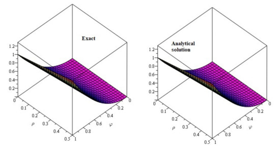
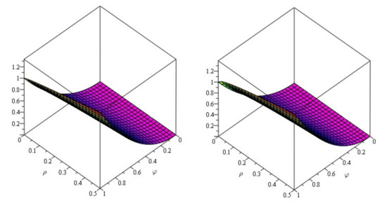
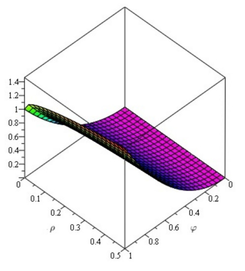
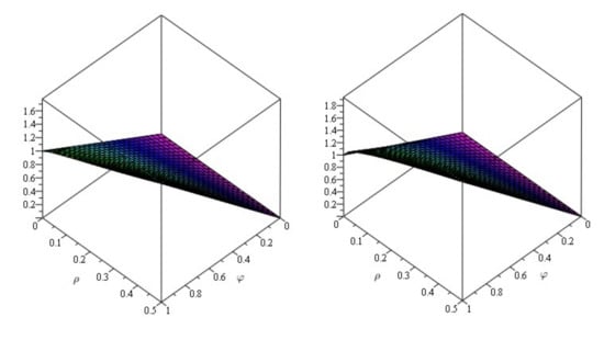
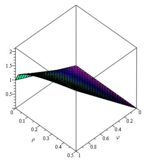
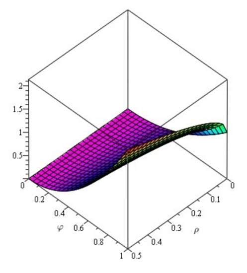
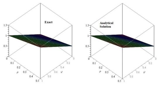
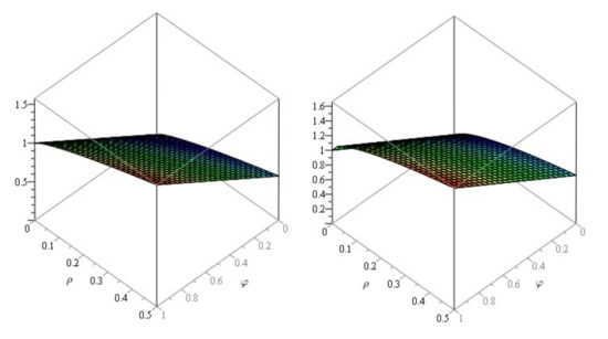
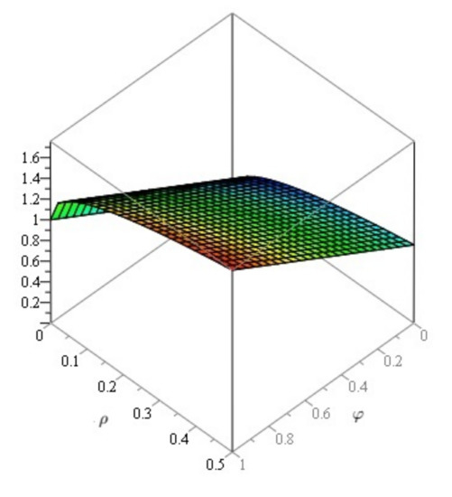
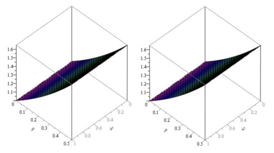
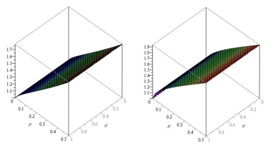
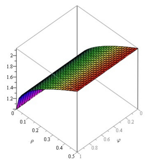
In Figure 1, represents the actual solution and the 2nd depicts the analytic result, which are in close contact. Figure 2 depicts fractional-order graphs at $\delta =0.8$ and $0.6$ for Problem 1. Similarly, in Figure 3, it is demonstrated that the Problem 1 fractional-order is $\delta =0.4$. The data demonstrate that the proposed method corresponds to the real solution for the given problem.

Problem 2.

Consider the fractional-order FP equation:

$$\frac{{\partial }^{\delta }}{\partial {\rho }^{\delta }}\nu (\phi ,\rho )+\frac{\partial }{\partial \phi }\left(\phi \nu (\phi ,\rho )\right)-\frac{{\partial }^2}{\partial {\phi }^2}\left(\frac{{\phi }^2}{2}\nu (\phi ,\rho )\right)=0,\phi ,\rho >0,\delta \in (0,1],$$

(18)

with the initial condition:

$$\nu (\phi ,0)=\phi .$$

On employing the ZZ transform, we get:

$$\mathcal{Z}\left\{\frac{{\partial }^{\delta }\nu }{\partial {\rho }^{\delta }}\right\}=\mathcal{Z}\left[-\frac{\partial }{\partial \phi }\left(\phi \nu (\phi ,\rho )\right)+\frac{{\partial }^2}{\partial {\phi }^2}\left(\frac{{\phi }^2}{2}\nu (\phi ,\rho )\right)\right],$$

(19)

By using the ZZ differentiation property, we have:

$$\frac{B\left(\delta \right)}{\left(1-\delta +\delta {\left(\frac{\varrho }{\varsigma }\right)}^{\delta }\right)}\mathcal{Z}\left\{\nu (\phi ,\rho )-\frac{\varrho }{\varsigma }\nu (\phi ,0)\right\}=\mathcal{Z}\left[-\frac{\partial }{\partial \phi }\left(\phi \nu (\phi ,\rho )\right)+\frac{{\partial }^2}{\partial {\phi }^2}\left(\frac{{\phi }^2}{2}\nu (\phi ,\rho )\right)\right].$$

(20)

On applying the inverse ZZ transform, we have:

$$\begin{array}{cc}\hfill & \nu (\phi ,\rho )=\nu (\phi ,0)+{\mathcal{Z}}^{-1}\left[\frac{\left(1-\delta +\delta {\left(\frac{\varrho }{\varsigma }\right)}^{\delta }\right)}{B\left(\delta \right)}\left\{\mathcal{Z}\left(-\frac{\partial }{\partial \phi }\left(\phi \nu (\phi ,\rho )\right)+\frac{{\partial }^2}{\partial {\phi }^2}\left(\frac{{\phi }^2}{2}\nu (\phi ,\rho )\right)\right)\right\}\right],\hfill \\ \hfill & \nu (\phi ,\rho )=\phi +{\mathcal{Z}}^{-1}\left[\frac{\left(1-\delta +\delta {\left(\frac{\varrho }{\varsigma }\right)}^{\delta }\right)}{B\left(\delta \right)}\left\{\mathcal{Z}\left(-\frac{\partial }{\partial \phi }\left(\phi \nu (\phi ,\rho )\right)+\frac{{\partial }^2}{\partial {\phi }^2}\left(\frac{{\phi }^2}{2}\nu (\phi ,\rho )\right)\right)\right\}\right].\hfill \end{array}$$

(21)

Using MDM, the solution in term of the infinite series $\nu (\phi ,\rho )$ can be expressed as:

$$\nu (\phi ,\rho )=\sum _{ȷ=0}^{\infty }{\nu }_{ȷ}(\phi ,\rho ).$$

(22)

$$\begin{array}{cc}\hfill & \sum _{ȷ=0}^{\infty }{\nu }_{ȷ}(\phi ,\rho )=\phi +{\mathcal{Z}}^{-1}\left[\frac{\left(1-\delta +\delta {\left(\frac{\varrho }{\varsigma }\right)}^{\delta }\right)}{B\left(\delta \right)}\mathcal{Z}\left[-\frac{\partial }{\partial \phi }\left(\phi \nu (\phi ,\rho )\right)+\frac{{\partial }^2}{\partial {\phi }^2}\left(\frac{{\phi }^2}{2}\nu (\phi ,\rho )\right)\right]\right].\hfill \end{array}$$

(23)

By comparing Equation (23) on both sides, we get:

$${\nu }_0(\phi ,\rho )=\phi ,$$

For $ȷ=0$

$${\nu }_1(\phi ,\rho )=\phi \frac{1}{B\left(\delta \right)}\left(1-\delta +\frac{\delta {\rho }^{\delta }}{\Gamma (\delta +1)}\right),$$

For $ȷ=1$

$${\nu }_2(\phi ,\rho )=\phi \frac{1}{{\left(\mathrm{B}\left(\delta \right)\right)}^2}\left({(1-\delta )}^2+\frac{2\delta (1-\delta ){\rho }^{\delta }}{\Gamma (\delta +1)}+\frac{{\delta }^2{\rho }^{2\delta }}{\Gamma (2\delta +1)}\right),$$

For $ȷ=2$

$$\begin{array}{cc}\hfill & {\nu }_3(\phi ,\rho )=\phi \frac{1}{{\left(\mathrm{B}\left(\delta \right)\right)}^3}\left({(1-\delta )}^3+\frac{3\delta {(1-\delta )}^2{\rho }^{\delta }}{\Gamma (\delta +1)}+\frac{{\delta }^2(1-\delta ){\rho }^{2\delta +1}}{\Gamma (2\delta +2)}+\frac{2{\delta }^2(1-\delta ){\rho }^{2\delta }}{\Gamma (2\delta +1)}+\frac{{\delta }^3{\rho }^{2\delta +1}}{\Gamma (2\delta +2)}\right).\hfill \end{array}$$

The MDM solution remaining components ${\nu }_{ȷ}$ with $(ȷ\ge 3)$ are simply determined.

$$\nu (\phi ,\rho )=\sum _{ȷ=0}^{\infty }{\nu }_{ȷ}(\phi ,\rho )={\nu }_0(\phi ,\rho )+{\nu }_1(\phi ,\rho )+{\nu }_2(\phi ,\rho )+{\nu }_3(\phi ,\rho )+\cdots .$$

$$\begin{array}{cc}\hfill & \nu (\phi ,\rho )=\phi +\phi \frac{1}{B\left(\delta \right)}\left(1-\delta +\frac{\delta {\rho }^{\delta }}{\Gamma (\delta +1)}\right)+\phi \frac{1}{{\left(\mathrm{B}\left(\delta \right)\right)}^2}\left({(1-\delta )}^2+\frac{2\delta (1-\delta ){\rho }^{\delta }}{\Gamma (\delta +1)}+\frac{{\delta }^2{\rho }^{2\delta }}{\Gamma (2\delta +1)}\right)\hfill \\ \hfill & +\phi \frac{1}{{\left(\mathrm{B}\left(\delta \right)\right)}^3}\left({(1-\delta )}^3+\frac{3\delta {(1-\delta )}^2{\rho }^{\delta }}{\Gamma (\delta +1)}+\frac{{\delta }^2(1-\delta ){\rho }^{2\delta +1}}{\Gamma (2\delta +2)}+\frac{2{\delta }^2(1-\delta ){\rho }^{2\delta }}{\Gamma (2\delta +1)}+\frac{{\delta }^3{\rho }^{2\delta +1}}{\Gamma (2\delta +2)}\right)+\cdots .\hfill \end{array}$$

The MDM solution at $\delta =1$ is:

$$\nu (\phi ,\rho )=\phi e^{\rho }.$$

(24)

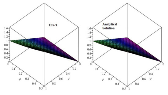
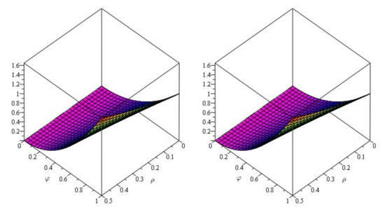
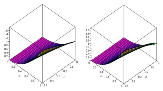
In Figure 4, represents the actual solution and the 2nd depicts the analytic result, which are in close contact. Figure 5 depicts fractional-order graphs at $\delta =0.8$ and $0.6$ for Problem 2. Similarly, in Figure 6, it is demonstrated that the Problem 2 fractional-order is $\delta =0.4$. The data demonstrate that the proposed method corresponds to the real solution for the given problem.

Problem 3.

Consider the fractional-order FP equation:

$$\frac{{\partial }^{\delta }}{\partial {\rho }^{\delta }}\nu (\phi ,\rho )+\frac{\partial }{\partial \phi }\left(\frac{4}{\phi }{\nu }^2(\phi ,\rho )\right)-\frac{\partial }{\partial \phi }\left(\frac{\phi }{3}\nu (\phi ,\rho )\right)-\frac{{\partial }^2}{\partial {\phi }^2}\left({\nu }^2(\phi ,\rho )\right)=0,\phi ,\rho >0,\delta \in (0,1],$$

(25)

with the initial condition:

$$\nu (\phi ,0)={\phi }^2.$$

On employing the ZZ transform, we get:

$$\mathcal{Z}\left\{\frac{{\partial }^{\delta }\nu }{\partial {\rho }^{\delta }}\right\}=\mathcal{Z}\left[\frac{\partial }{\partial \phi }\left(\frac{\phi }{3}\nu (\phi ,\rho )\right)+\frac{{\partial }^2}{\partial {\phi }^2}\left({\nu }^2(\phi ,\rho )\right)-\frac{\partial }{\partial \phi }\left(\frac{4}{\phi }{\nu }^2(\phi ,\rho )\right)\right].$$

(26)

By using the ZZ differentiation property, we have:

$$\frac{B\left(\delta \right)}{\left(1-\delta +\delta {\left(\frac{\varrho }{\varsigma }\right)}^{\delta }\right)}\mathcal{Z}\left\{\nu (\phi ,\rho )-\frac{\varrho }{\varsigma }\nu (\phi ,0)\right\}=\mathcal{Z}\left[\frac{\partial }{\partial \phi }\left(\frac{\phi }{3}\nu (\phi ,\rho )\right)+\frac{{\partial }^2}{\partial {\phi }^2}\left({\nu }^2(\phi ,\rho )\right)-\frac{\partial }{\partial \phi }\left(\frac{4}{\phi }{\nu }^2(\phi ,\rho )\right)\right].$$

(27)

On applying the inverse ZZ transform, we have:

$$\begin{array}{cc}\hfill & \nu (\phi ,\rho )=\nu (\phi ,0)+{\mathcal{Z}}^{-1}\left[\frac{\left(1-\delta +\delta {\left(\frac{\varrho }{\varsigma }\right)}^{\delta }\right)}{B\left(\delta \right)}\left\{\mathcal{Z}\left(\frac{\partial }{\partial \phi }\left(\frac{\phi }{3}\nu (\phi ,\rho )\right)+\frac{{\partial }^2}{\partial {\phi }^2}\left({\nu }^2(\phi ,\rho )\right)-\frac{\partial }{\partial \phi }\left(\frac{4}{\phi }{\nu }^2(\phi ,\rho )\right)\right)\right\}\right],\hfill \\ \hfill & \nu (\phi ,\rho )={\phi }^2+{\mathcal{Z}}^{-1}\left[\frac{\left(1-\delta +\delta {\left(\frac{\varrho }{\varsigma }\right)}^{\delta }\right)}{B\left(\delta \right)}\left\{\mathcal{Z}\left(\frac{\partial }{\partial \phi }\left(\frac{\phi }{3}\nu (\phi ,\rho )\right)+\frac{{\partial }^2}{\partial {\phi }^2}\left({\nu }^2(\phi ,\rho )\right)-\frac{\partial }{\partial \phi }\left(\frac{4}{\phi }{\nu }^2(\phi ,\rho )\right)\right)\right\}\right].\hfill \end{array}$$

(28)

Now, we assume that the infinite series from the function $\nu (\phi ,\rho )$, which is unknown, has the solution as:

$$\nu (\phi ,\rho )=\sum _{ȷ=0}^{\infty }{\nu }_{ȷ}(\phi ,\rho ).$$

(29)

The nonlinear terms are therefore described by the Adomian polynomial ${\nu }^2={\sum }_{ȷ=0}^{\infty }{\mathcal{A}}_{ȷ}$. Applying particular concepts, Equation (28) can be expressed as:

$$\begin{array}{cc}\hfill & \sum _{ȷ=0}^{\infty }{\nu }_{ȷ}(\phi ,\rho )=\nu (\phi ,0)+{\mathcal{Z}}^{-1}\left[\frac{\left(1-\delta +\delta {\left(\frac{\varrho }{\varsigma }\right)}^{\delta }\right)}{B\left(\delta \right)}\mathcal{Z}\left[\frac{\partial }{\partial \phi }\left(\frac{\phi }{3}\nu (\phi ,\rho )\right)+\sum _{ȷ=0}^{\infty }{\mathcal{A}}_{ȷ}\right]\right],\hfill \\ \hfill & \sum _{ȷ=0}^{\infty }{\nu }_{ȷ}(\phi ,\rho )={\phi }^2+{\mathcal{Z}}^{-1}\left[\frac{\left(1-\delta +\delta {\left(\frac{\varrho }{\varsigma }\right)}^{\delta }\right)}{B\left(\delta \right)}\mathcal{Z}\left[\frac{\partial }{\partial \phi }\left(\frac{\phi }{3}\nu (\phi ,\rho )\right)+\sum _{ȷ=0}^{\infty }{\mathcal{A}}_{ȷ}\right]\right].\hfill \end{array}$$

(30)

Now, by Adomian polynomials $\mathcal{A}$, the non-linear term is decomposed as,

$${\mathcal{A}}_0={\nu }_0^2,{\mathcal{A}}_1=2{\nu }_0{\nu }_1,{\mathcal{A}}_2=2{\nu }_0{\nu }_2+{\left({\nu }_2\right)}^2.$$

By comparing Equation (30) both sides, we get:

$${\nu }_0(\phi ,\rho )={\phi }^2,$$

On $ȷ=0$

$${\nu }_1(\phi ,\rho )={\phi }^2\frac{1}{B\left(\delta \right)}\left(1-\delta +\frac{\delta {\rho }^{\delta }}{\Gamma (\delta +1)}\right),$$

On $ȷ=1$

$${\nu }_2(\phi ,\rho )={\phi }^2\frac{1}{{\left(\mathrm{B}\left(\delta \right)\right)}^2}\left({(1-\delta )}^2+\frac{2\delta (1-\delta ){\rho }^{\delta }}{\Gamma (\delta +1)}+\frac{{\delta }^2{\rho }^{2\delta }}{\Gamma (2\delta +1)}\right),$$

On $ȷ=2$

$${\nu }_3(\phi ,\rho )={\phi }^2\frac{1}{{\left(\mathrm{B}\left(\delta \right)\right)}^3}\left({(1-\delta )}^3+\frac{3\delta {(1-\delta )}^2{\rho }^{\delta }}{\Gamma (\delta +1)}+\frac{{\delta }^2(1-\delta ){\rho }^{2\delta +1}}{\Gamma (2\delta +2)}+\frac{2{\delta }^2(1-\delta ){\rho }^{2\delta }}{\Gamma (2\delta +1)}+\frac{{\delta }^3{\rho }^{2\delta +1}}{\Gamma (2\delta +2)}\right).$$

The MDM solution remaining components ${\nu }_{ȷ}$ with $(ȷ\ge 3)$, are simply calculated.

$$\nu (\phi ,\rho )=\sum _{ȷ=0}^{\infty }{\nu }_{ȷ}(\phi ,\rho )={\nu }_0(\phi ,\rho )+{\nu }_1(\phi ,\rho )+{\nu }_2(\phi ,\rho )+{\nu }_3(\phi ,\rho )+\cdots .$$

$$\begin{array}{c}\hfill \nu (\phi ,\rho )={\phi }^2+{\phi }^2\frac{1}{B\left(\delta \right)}\left(1-\delta +\frac{\delta {\rho }^{\delta }}{\Gamma (\delta +1)}\right)+{\phi }^2\frac{1}{{\left(\mathrm{B}\left(\delta \right)\right)}^2}\left({(1-\delta )}^2+\frac{2\delta (1-\delta ){\rho }^{\delta }}{\Gamma (\delta +1)}+\frac{{\delta }^2{\rho }^{2\delta }}{\Gamma (2\delta +1)}\right)+\\ \hfill {\phi }^2\frac{1}{{\left(\mathrm{B}\left(\delta \right)\right)}^3}\left({(1-\delta )}^3+\frac{3\delta {(1-\delta )}^2{\rho }^{\delta }}{\Gamma (\delta +1)}+\frac{{\delta }^2(1-\delta ){\rho }^{2\delta +1}}{\Gamma (2\delta +2)}+\frac{2{\delta }^2(1-\delta ){\rho }^{2\delta }}{\Gamma (2\delta +1)}+\frac{{\delta }^3{\rho }^{2\delta +1}}{\Gamma (2\delta +2)}\right)+\cdots .\end{array}$$

The MDM solution at $\delta =1$ is:

$$\nu (\phi ,\rho )={\phi }^2{e}^{\rho }.$$

(31)

In Figure 7, represents the actual solution and the 2nd depicts the analytic result, which are in close contact. Figure 8 depicts fractional-order graphs at $\delta =0.8$ and $0.6$ for Problem 3. Similarly, in Figure 9, it is demonstrated that the Problem 3 fractional-order is $\delta =0.4$. The data demonstrate that the proposed method corresponds to the real solution for the given problem.

Problem 4.

Consider the fractional-order FP equation:

$$\frac{{\partial }^{\delta }}{\partial {\rho }^{\delta }}\nu (\phi ,\rho )-\frac{\partial }{\partial \phi }\nu (\phi ,\rho )-\frac{{\partial }^2}{\partial {\phi }^2}\nu (\phi ,\rho )=0,\rho >0,\delta \in (0,1],$$

(32)

with the initial condition:

$$\nu (\phi ,0)=\phi .$$

On employing the ZZ transform, we get:

$$\mathcal{Z}\left\{\frac{{\partial }^{\delta }\nu }{\partial {\rho }^{\delta }}\right\}=\mathcal{Z}\left[\frac{\partial }{\partial \phi }\nu (\phi ,\rho )+\frac{{\partial }^2}{\partial {\phi }^2}\nu (\phi ,\rho )\right],$$

(33)

By using the ZZ differentiation property, we have:

$$\frac{B\left(\delta \right)}{\left(1-\delta +\delta {\left(\frac{\varrho }{\varsigma }\right)}^{\delta }\right)}\mathcal{Z}\left\{\nu (\phi ,\rho )-\frac{\varrho }{\varsigma }\nu (\phi ,0)\right\}=\mathcal{Z}\left[\frac{\partial }{\partial \phi }\nu (\phi ,\rho )+\frac{{\partial }^2}{\partial {\phi }^2}\nu (\phi ,\rho )\right].$$

(34)

On applying the inverse ZZ transform, we have:

$$\begin{array}{cc}\hfill & \nu (\phi ,\rho )=\nu \left(0\right)+{\mathcal{Z}}^{-1}\left[\frac{\left(1-\delta +\delta {\left(\frac{\varrho }{\varsigma }\right)}^{\delta }\right)}{B\left(\delta \right)}\left\{\mathcal{Z}\left(\frac{\partial }{\partial \phi }\nu (\phi ,\rho )+\frac{{\partial }^2}{\partial {\phi }^2}\nu (\phi ,\rho )\right)\right\}\right],\hfill \\ \hfill & \nu (\phi ,\rho )=\phi +{\mathcal{Z}}^{-1}\left[\frac{\left(1-\delta +\delta {\left(\frac{\varrho }{\varsigma }\right)}^{\delta }\right)}{B\left(\delta \right)}\left\{\mathcal{Z}\left(\frac{\partial }{\partial \phi }\nu (\phi ,\rho )+\frac{{\partial }^2}{\partial {\phi }^2}\nu (\phi ,\rho )\right)\right\}\right].\hfill \end{array}$$

(35)

Using MDM, the solution in terms of the infinite series $\nu (\phi ,\rho )$ can be expressed as:

$$\nu (\phi ,\rho )=\sum _{ȷ=0}^{\infty }{\nu }_{ȷ}(\phi ,\rho ).$$

(36)

$$\begin{array}{cc}\hfill & \sum _{ȷ=0}^{\infty }{\nu }_{ȷ}(\phi ,\rho )=\phi +{\mathcal{Z}}^{-1}\left[\frac{\left(1-\delta +\delta {\left(\frac{\varrho }{\varsigma }\right)}^{\delta }\right)}{B\left(\delta \right)}\mathcal{Z}\left[\frac{\partial }{\partial \phi }\nu (\phi ,\rho )+\frac{{\partial }^2}{\partial {\phi }^2}\nu (\phi ,\rho )\right]\right].\hfill \end{array}$$

(37)

By comparing Equation (37) on both sides, we get:

$${\nu }_0(\phi ,\rho )=\phi ,$$

For $ȷ=0$

$${\nu }_1(\phi ,\rho )=\frac{1}{B\left(\delta \right)}\left(1-\delta +\frac{\delta {\rho }^{\delta }}{\Gamma (\delta +1)}\right),$$

For $ȷ=1$

$${\nu }_2(\phi ,\rho )=0,$$

For $ȷ=2$

$$\begin{array}{cc}\hfill & {\nu }_3(\phi ,\rho )=0.\hfill \end{array}$$

The MDM solution remaining components ${\nu }_{ȷ}$ with $(ȷ\ge 3)$ are simply calculated.

$$\nu (\phi ,\rho )=\sum _{ȷ=0}^{\infty }{\nu }_{ȷ}(\phi ,\rho )={\nu }_0(\phi ,\rho )+{\nu }_1(\phi ,\rho )+{\nu }_2(\phi ,\rho )+{\nu }_3(\phi ,\rho )+\cdots .$$

$$\begin{array}{cc}\hfill & \nu (\phi ,\rho )=\phi +\frac{1}{B\left(\delta \right)}\left(1-\delta +\frac{\delta {\rho }^{\delta }}{\Gamma (\delta +1)}\right)+0+0+\cdots .\hfill \end{array}$$

The MDM solution at $\delta =1$ is:

$$\nu (\phi ,\rho )=\phi +\rho .$$

(38)

In Figure 10, represents the actual solution and the 2nd depicts the analytic result, which are in close contact. Figure 11 depicts fractional-order graphs at $\delta =0.8$ and $0.6$ for Problem 4. Similarly, in Figure 12, it is demonstrated that the Problem 4 fractional-order is $\delta =0.4$. The data demonstrate that the proposed method corresponds to the real solution for the given problem.

Problem 5.

Consider the fractional-order FP equation:

$$\frac{{\partial }^{\delta }}{\partial {\rho }^{\delta }}\nu (\phi ,\rho )-(1-\phi )\frac{\partial }{\partial \phi }\nu (\phi ,\rho )-\left(e^{\rho }{\phi }^2\right)\frac{{\partial }^2}{\partial {\phi }^2}\nu (\phi ,\rho )=0,\rho >0,\delta \in (0,1],$$

(39)

with the initial condition:

$$\nu (\phi ,0)=1+\phi .$$

On employing the ZZ transform, we get:

$$\mathcal{Z}\left\{\frac{{\partial }^{\delta }\nu }{\partial {\rho }^{\delta }}\right\}=\mathcal{Z}\left[(1-\phi )\frac{\partial }{\partial \phi }\nu (\phi ,\rho )+\left(e^{\rho }{\phi }^2\right)\frac{{\partial }^2}{\partial {\phi }^2}\nu (\phi ,\rho )\right].$$

(40)

By using the ZZ differentiation property, we have:

$$\frac{B\left(\delta \right)}{\left(1-\delta +\delta {\left(\frac{\varrho }{\varsigma }\right)}^{\delta }\right)}\mathcal{Z}\left\{\nu (\phi ,\rho )-\frac{\varrho }{\varsigma }\nu (\phi ,0)\right\}=\mathcal{Z}\left[(1-\phi )\frac{\partial }{\partial \phi }\nu (\phi ,\rho )+\left(e^{\rho }{\phi }^2\right)\frac{{\partial }^2}{\partial {\phi }^2}\nu (\phi ,\rho )\right].$$

(41)

On applying the inverse ZZ transform, we have:

$$\begin{array}{cc}\hfill & \nu (\phi ,\rho )=\nu \left(0\right)+{\mathcal{Z}}^{-1}\left[\frac{\left(1-\delta +\delta {\left(\frac{\varrho }{\varsigma }\right)}^{\delta }\right)}{B\left(\delta \right)}\left\{\mathcal{Z}\left((1-\phi )\frac{\partial }{\partial \phi }\nu (\phi ,\rho )+\left(e^{\rho }{\phi }^2\right)\frac{{\partial }^2}{\partial {\phi }^2}\nu (\phi ,\rho )\right)\right\}\right],\hfill \\ \hfill & \nu (\phi ,\rho )=(1+\phi )+{\mathcal{Z}}^{-1}\left[\frac{\left(1-\delta +\delta {\left(\frac{\varrho }{\varsigma }\right)}^{\delta }\right)}{B\left(\delta \right)}\left\{\mathcal{Z}\left((1-\phi )\frac{\partial }{\partial \phi }\nu (\phi ,\rho )+\left(e^{\rho }{\phi }^2\right)\frac{{\partial }^2}{\partial {\phi }^2}\nu (\phi ,\rho )\right)\right\}\right].\hfill \end{array}$$

(42)

The solution in terms of infinite sequence $\nu (\phi ,\rho )$ by means of MDM is:

$$\nu (\phi ,\rho )=\sum _{ȷ=0}^{\infty }{\nu }_{ȷ}(\phi ,\rho ).$$

(43)

$$\begin{array}{cc}\hfill & \sum _{ȷ=0}^{\infty }{\nu }_{ȷ}(\phi ,\rho )=(1+\phi )+{\mathcal{Z}}^{-1}\left[\frac{\left(1-\delta +\delta {\left(\frac{\varrho }{\varsigma }\right)}^{\delta }\right)}{B\left(\delta \right)}\mathcal{Z}\left[(1-\phi )\frac{\partial }{\partial \phi }\nu (\phi ,\rho )+\left(e^{\rho }{\phi }^2\right)\frac{{\partial }^2}{\partial {\phi }^2}\nu (\phi ,\rho )\right]\right].\hfill \end{array}$$

(44)

By comparing Equation (44) on both sides, we get:

$${\nu }_0(\phi ,\rho )=1+\phi ,$$

For $ȷ=0$

$${\nu }_1(\phi ,\rho )=(1+\phi )\frac{1}{B\left(\delta \right)}\left(1-\delta +\frac{\delta {\rho }^{\delta }}{\Gamma (\delta +1)}\right).$$

For $ȷ=1$

$${\nu }_2(\phi ,\rho )=(1+\phi )\frac{1}{{\left(\mathrm{B}\left(\delta \right)\right)}^2}\left({(1-\delta )}^2+\frac{2\delta (1-\delta ){\rho }^{\delta }}{\Gamma (\delta +1)}+\frac{{\delta }^2{\rho }^{2\delta }}{\Gamma (2\delta +1)}\right).$$

For $ȷ=2$

$$\begin{array}{cc}\hfill & {\nu }_3(\phi ,\rho )=(1+\phi )\frac{1}{{\left(\mathrm{B}\left(\delta \right)\right)}^3}\left({(1-\delta )}^3+\frac{3\delta {(1-\delta )}^2{\rho }^{\delta }}{\Gamma (\delta +1)}+\frac{{\delta }^2(1-\delta ){\rho }^{2\delta +1}}{\Gamma (2\delta +2)}+\frac{2{\delta }^2(1-\delta ){\rho }^{2\delta }}{\Gamma (2\delta +1)}+\frac{{\delta }^3{\rho }^{2\delta +1}}{\Gamma (2\delta +2)}\right).\hfill \end{array}$$

The MDM solution remaining components ${\nu }_{ȷ}$ with $(ȷ\ge 3)$ are easily calculated.

$$\nu (\phi ,\rho )=\sum _{ȷ=0}^{\infty }{\nu }_{ȷ}(\phi ,\rho )={\nu }_0(\phi ,\rho )+{\nu }_1(\phi ,\rho )+{\nu }_2(\phi ,\rho )+{\nu }_3(\phi ,\rho )+\cdots .$$

$$\begin{array}{cc}\hfill & \nu (\phi ,\rho )=(1+\phi )+(1+\phi )\frac{1}{B\left(\delta \right)}\left(1-\delta +\frac{\delta {\rho }^{\delta }}{\Gamma (\delta +1)}\right)+(1+\phi )\frac{1}{{\left(\mathrm{B}\left(\delta \right)\right)}^2}\left({(1-\delta )}^2+\frac{2\delta (1-\delta ){\rho }^{\delta }}{\Gamma (\delta +1)}+\frac{{\delta }^2{\rho }^{2\delta }}{\Gamma (2\delta +1)}\right)\hfill \\ \hfill & +(1+\phi )\frac{1}{{\left(\mathrm{B}\left(\delta \right)\right)}^3}\left({(1-\delta )}^3+\frac{3\delta {(1-\delta )}^2{\rho }^{\delta }}{\Gamma (\delta +1)}+\frac{{\delta }^2(1-\delta ){\rho }^{2\delta +1}}{\Gamma (2\delta +2)}+\frac{2{\delta }^2(1-\delta ){\rho }^{2\delta }}{\Gamma (2\delta +1)}+\frac{{\delta }^3{\rho }^{2\delta +1}}{\Gamma (2\delta +2)}\right)+\cdots .\hfill \end{array}$$

The MDM solution at $\delta =1$ is:

$$\nu (\phi ,\rho )=e^{\rho }(1+\phi ).$$

(45)

In Figure 13, represents the actual solution and the 2nd depicts the analytic result, which are in close contact. Figure 14 depicts fractional-order graphs at $\delta =0.8$ and $0.6$ for Problem 5. Similarly, in Figure 15, it is demonstrated that the Problem 5 fractional-order is $\delta =0.4$. The data demonstrate that the proposed method corresponds to the real solution for the given problem.

5. Conclusions

In this study, we successfully apply the modified decomposition method to solve the fractional-order Fokker-Planck equations analytically. Five different issues involving fractional-order Fokker-Planck equations were explored to demonstrate the viability of the recommended method. The numerical simulations demonstrate that the outcomes of our method are in close accordance with the exact answer. For getting numerical solutions to fractional-order Fokker-Planck equations, the current method is relatively simple, efficient, and appropriate. The primary advantage of the proposed approach is the series form solution, which rapidly converges to the exact solution.

References

- Din, A.; Khan, F.M.; Khan, Z.U.; Yusuf, A.; Munir, T. The mathematical study of climate change model under nonlocal fractional derivative. Partial. Differ. Equ. Appl. Math. 2022, 5, 100204. [Google Scholar] [CrossRef]
- Jajarmi, A.; Baleanu, D.; Zarghami, V.K.; Mobayen, S. A general fractional formulation and tracking control for immunogenic tumor dynamics. Math. Methods Appl. Sci. 2022, 45, 667–680. [Google Scholar] [CrossRef]
- Modanli, M.; Goktepe, E.; Akgul, A.; Alsallami, S.A.; Khalil, E.M. Two approximation methods for fractional order Pseudo-Parabolic differential equations. Alex. Eng. J. 2022, 61, 10333–10339. [Google Scholar] [CrossRef]
- Erturk, V.S.; Godwe, E.; Baleanu, D.; Kumar, P.; Asad, J.; Jajarmi, A. Novel fractional-order Lagrangian to describe motion of beam on nanowire. Acta Phys. Pol. A 2021, 140, 265–272. [Google Scholar] [CrossRef]
- Jajarmi, A.; Baleanu, D.; Vahid, K.Z.; Pirouz, H.M.; Asad, J.H. A new and general fractional Lagrangian approach: A capacitor microphone case study. Results Phys. 2021, 31, 104950. [Google Scholar] [CrossRef]
- Khashi’ie, N.S.; Waini, I.; Zainal, N.A.; Hamzah, K.; Mohd Kasim, A.R. Hybrid nanofluid flow past a shrinking cylinder with prescribed surface heat flux. Symmetry 2020, 12, 1493. [Google Scholar] [CrossRef]
- Podlubny, I. Fractional Differential Equations; Academic Press: San Diego, CA, USA, 1999. [Google Scholar]
- Millar, K.S.; Ross, B. An Introduction to the Fractional Calculus and Fractional Differential Equations; Wiley: New York, NY, USA, 1993. [Google Scholar]
- Caputo, M. Linear models of dissipation whose Q is almost frequency independent: Part II. Geophys. J. Int. 1967, 13, 529–539. [Google Scholar] [CrossRef]
- Al-Smadi, M. Simplified iterative reproducing kernel method for handling time-fractional BVPs with error estimation. Ain Shams Eng. J. 2018, 9, 2517–2525. [Google Scholar] [CrossRef]
- Alqhtani, M.; Saad, K.; Shah, R.; Weera, W.; Hamanah, W. Analysis of the Fractional-Order Local Poisson Equation in Fractal Porous Media. Symmetry 2022, 14, 1323. [Google Scholar] [CrossRef]
- Singh, C.S.; Singh, H.; Singh, V.K.; Singh, O.P. Fractional order operational matrix methods for fractional singular integro-differential equation. Appl. Math. Model. 2016, 40, 10705–10718. [Google Scholar] [CrossRef]
- Mukhtar, S.; Noor, S. The Numerical Investigation of a Fractional-Order Multi-Dimensional Model of Navier-Stokes Equation via Novel Techniques. Symmetry 2022, 14, 1102. [Google Scholar] [CrossRef]
- Khan, H.; Farooq, U.; Baleanu, D.; Kumam, P.; Arif, M. Analytical solutions of (2+ time fractional order) dimensional physical models, using modified decomposition method. Appl. Sci. 2019, 10, 122. [Google Scholar] [CrossRef]
- Shah, R.; Khan, H.; Baleanu, D. Fractional Whitham-Broer-Kaup equations within modified analytical approaches. Axioms 2019, 8, 125. [Google Scholar] [CrossRef]
- Shah, R.; Khan, H.; Kumam, P.; Arif, M. An analytical technique to solve the system of nonlinear fractional partial differential equations. Mathematics 2019, 7, 505. [Google Scholar] [CrossRef]
- Alaoui, M.K.; Fayyaz, R.; Khan, A.; Abdo, M.S. Analytical Investigation of Noyes-Field Model for Time-Fractional Belousov-Zhabotinsky Reaction. Complexity 2021, 2021, 3248376. [Google Scholar] [CrossRef]
- Areshi, M.; Khan, A.; Nonlaopon, K. Analytical investigation of fractional-order Newell-Whitehead-Segel equations via a novel transform. AIMS Math. 2022, 7, 6936–6958. [Google Scholar] [CrossRef]
- Aboodh, K.S. Application of new transform “Aboodh Transform” to partial differential equations. Glob. J. Pure Appl. Math. 2014, 10, 249–254. [Google Scholar]
- Aboodh, K.S. Solving fourth order parabolic PDE with variable coefficients using Aboodh transform homotopy perturbation method. Pure Appl. Math. J. 2015, 4, 219–224. [Google Scholar] [CrossRef]
- Jena, R.M.; Chakraverty, S.; Baleanu, D.; Alqurashi, M.M. New aspects of ZZ transform to fractional operators with Mittag-Leffler kernel. Front. Phys. 2020, 8, 352. [Google Scholar] [CrossRef]
- Riabi, L.; Belghaba, K.; Cherif, M.H.; Ziane, D. Homotopy perturbation method combined with ZZ transform to solve some nonlinear fractional differential equations. Int. J. Anal. Appl. 2019, 17, 406–419. [Google Scholar]
- Zafar, Z.U.A. Application of ZZ transform method on some fractional differential equations. Int. J. Adv. Eng. Glob. Technol. 2016, 4, 1355–1363. [Google Scholar]
- Atangana, A.; Baleanu, D. New fractional derivatives with nonlocal and non-singular kernel: Theory and application to heat transfer model. Therm. Sci. 2016, 20, 763–769. [Google Scholar] [CrossRef]
- Nonlaopon, K.; Naeem, M.; Zidan, A.M.; Alsanad, A.; Gumaei, A. Numerical Investigation of the Time-Fractional Whitham-Broer-Kaup Equation Involving without Singular Kernel Operators. Complexity 2021, 2021, 7979365. [Google Scholar] [CrossRef]
- Aljahdaly, N.; Shah, R.; Naeem, M.; Arefin, M. A Comparative Analysis of Fractional Space-Time Advection-Dispersion Equation via Semi-Analytical Methods. J. Funct. Spaces 2022, 2022, 4856002. [Google Scholar] [CrossRef]
- Shah, N.A.; Alyousef, H.A.; El-Tantawy, S.A.; Chung, J.D. Analytical Investigation of Fractional-Order Korteweg-De-Vries-Type Equations under Atangana-Baleanu-Caputo Operator: Modeling Nonlinear Waves in a Plasma and Fluid. Symmetry 2022, 14, 739. [Google Scholar] [CrossRef]
- Wazwaz, A.M. A reliable modification of Adomian decomposition method. Appl. Math. Comput. 1999, 102, 77–86. [Google Scholar] [CrossRef]
- Mofarreh, F.; Zidan, A.; Naeem, M.; Ullah, R.; Nonlaopon, K. Analytical Analysis of Fractional-Order Physical Models via a Caputo-Fabrizio Operator. J. Funct. Spaces 2021, 2021, 7250308. [Google Scholar] [CrossRef]
- Thabet, H.; Kendre, S. New modification of Adomian decomposition method for solving a system of nonlinear fractional partial differential equations. Int. J. Adv. Appl. Math. Mech. 2019, 6, 1–13. [Google Scholar]
- Firoozjaee, M.A.; Yousefi, S.A.; Jafari, H. A numerical approach to Fokker-Planck equation with space- and time-fractional and non fractional derivatives. Match Commun. Math. Comput. Chem. 2015, 74, 449–464. [Google Scholar]
- Aljahdaly, N.H.; Akgul, A.; Mahariq, I.; Kafle, J. A comparative analysis of the fractional-order coupled Korteweg-De Vries equations with the Mittag-Leffler law. J. Math. 2022, 2022, 8876149. [Google Scholar] [CrossRef]
- Momani, S.; Arqub, O.A.; Freihat, A.; Al-Smadi, M. Analytical approximations for Fokker-Planck equations of fractional order in multistep schemes. Appl. Comput. Math. 2016, 15, 319–330. [Google Scholar]
- Deng, W. Numerical algorithm for the time fractional Fokker-Planck equation. J. Comput. Phys. 2007, 227, 1510–1522. [Google Scholar] [CrossRef]
- Odibat, Z.; Momani, S. Numerical solution of FokkerPlanck equation with space-and time-fractional derivatives. Phys. Lett. A 2007, 369, 349–358. [Google Scholar] [CrossRef]
- Adomian, G. Solution of physical problems by decomposition. Comput. Math. Appl. 1994, 27, 145–154. [Google Scholar] [CrossRef]
- Adomian, G. Solutions of Nonlinear PDE. Appl. Math. Lett. 1998, 11, 121–123. [Google Scholar] [CrossRef]
- Adomian, G. Analytical solution of Navier-Stokes flow of a viscous compressible fluid, Found. Phys. Lett. 1995, 8, 389–400. [Google Scholar]
- Cherruault, Y. A new approach to solve a diffusion-convection problem. Kybernetes 2002, 31, 536–549. [Google Scholar]
- Basto, M.; Semiao, V.; Calheiros, F.L. Numerical study of modified Adomian’s method applied to Burgers equation. J. Comput. Appl. Math. 2007, 206, 927–949. [Google Scholar] [CrossRef]
- Krasnoschok, M.; Pata, V.; Siryk, S.V.; Vasylyeva, N. A subdiffusive Navier-Stokes-Voigt system. Phys. D Nonlinear Phenom. 2020, 409, 132503. [Google Scholar] [CrossRef]
- Siryk, S.V.; Salnikov, N.N. Numerical solution of Burgers’ equation by Petrov-Galerkin method with adaptive weighting functions. J. Autom. Inf. Sci. 2012, 44, 50–67. [Google Scholar] [CrossRef]
- Roos, H.-G.; Stynes, M.; Tobiska, L. Robust Numerical Methods for Singularly Perturbed Differential Equations; Springer: Berlin/Heidelberg, Germany, 2008; 604p. [Google Scholar]
- NSalnikov, N.; Siryk, S.V. Construction of Weight Functions of the Petrov-Galerkin Method for Convection-Diffusion-Reaction Equations in the Three-Dimensional Case. Cybern. Syst. Anal. 2014, 50, 805–814. [Google Scholar] [CrossRef]
- John, V.; Knobloch, P.; Novo, J. Finite elements for scalar convection-dominated equations and incompressible flow problems: A never ending story. Comput. Vis. Sci. 2018, 19, 47–63. [Google Scholar] [CrossRef]
- Siryk, S.V. A note on the application of the Guermond-Pasquetti mass lumping correction technique for convection-diffusion problems. J. Comput. Phys. 2019, 376, 1273–1291. [Google Scholar] [CrossRef]
- Ahmad, S.; Ullah, A.; Akgul, A.; De la Sen, M. A Novel Homotopy Perturbation Method with Applications to Nonlinear Fractional Order KdV and Burger Equation with Exponential-Decay Kernel. J. Funct. Spaces 2021, 2021, 8770488. [Google Scholar] [CrossRef]
- Xu, Y. Similarity solution and heat transfer characteristics for a class of nonlinear convection-diffusion equation with initial value conditions. Math. Probl. Eng. 2019, 2019, 3467276. [Google Scholar] [CrossRef]
- Sun, H.; Zhang, Y.; Baleanu, D.; Chen, W.; Chen, Y. A new collection of real world applications of fractional calculus in science and engineering. Commun. Nonlinear Sci. Numer. Simul. 2018, 64, 213–231. [Google Scholar] [CrossRef]
- Krasnoschok, M.; Pata, V.; Siryk, S.V.; Vasylyeva, N. Equivalent definitions of Caputo derivatives and applications to subdiffusion equations. Dyn. Partial. Differ. Equ. 2020, 17, 383–402. [Google Scholar] [CrossRef]
- Diethelm, K.; Garrappa, R.; Stynes, M. Good (and Not So Good) practices in computational methods for fractional calculus. Mathematics 2020, 8, 324. [Google Scholar] [CrossRef]
- Adomian, G. A review of the decomposition method in applied mathematics. J. Math. Anal. Appl. 1988, 135, 501–544. [Google Scholar] [CrossRef]
- Shah, R.; Khan, H.; Arif, M.; Kumam, P. Application of Laplace-Adomian decomposition method for the analytical solution of third-order dispersive fractional partial differential equations. Entropy 2019, 21, 335. [Google Scholar] [CrossRef]
Publisher’s Note: MDPI stays neutral with regard to jurisdictional claims in published maps and institutional affiliations. |
© 2022 by the authors. Licensee MDPI, Basel, Switzerland. This article is an open access article distributed under the terms and conditions of the Creative Commons Attribution (CC BY) license (https://creativecommons.org/licenses/by/4.0/).