Abstract
This work proposes a valuable and successful strategy for approximating the solutions to the Bagley–Torvik system, which plays an essential role in fractional calculus. The Caputo sense is used to derive the basic conformable fractional. The Bagley–Torvik problem is numerically solved in this study using an effective symmetric projection method. From this symmetry, there are some interesting original results. The proposed approach has two key benefits. We began by converting the connected fractional Bagley–Torvik equations into two fractional-order Bagley–Torvik equations, which we then solved using the current method. Second, two linear equation systems are solved to obtain approximate solutions.
1. Introduction
Because of its applications, fractional calculus has received a lot of attention from mathematicians and scientists in recent decades. Numerous investigators have shown the ramifications of fractional order derivative as a different physical phenomenon. Nonlinear dynamics, Maclaurin theory, theoretical physics, biomedicine, polymeric materials, dynamical mechanics, electron microscopy, transportation system, discharge and viscoelasticity, confusion and geometrisc, identification and modeling, filtration, financial system, and finance are all implementations of fractional differential problems.
The Bagley–Torvik equation plays a critical part in fractional differential equations, because it appears in the mathematical model of the movement of a big thin plate immersed in a Newtonian fluid. Torvik and Bagley introduced this fractional differential equation for the first time in 1984. The researchers stated that the fractional derivative is usually noticed in the behavior of real materials (see [1]). The authors of [2] investigated the stability conditions for linear matrix inequality in fractional order systems. In [3], a novel approach for fractional-order inputted systems is presented that is deduced from the guardian map and described as a family of monoparametric pseudo-polynomials. Reference [4] discussed a numerical approximation to a class of variable-order fractional functional boundary value problems.
The Bagley–Torvik equation has been investigated by a number of researchers using various approximate numerical methods. The goal of [5] is to propose and study a novel operational Tau approach with a high order to achieve the numerical solution to a Bagley–Torvik problem that uses Chebyshev polynomials as basis functions. Some derivatives of these equations’ solutions have a singularity at their origin, according to the author. The authors of [6] proposed a new numerical method for approximating the solution to the Bagley–Torvik problem. The fundamental goal of their strategy is to obtain a more general approximation solution in the form of Müntz–Legendre polynomials. The authors of [7] proposed an effective numerical technique founded on shifted Chebyshev polynomials for deriving numerical solutions to the Bagley–Torvik equation. The authors of [8] considered restructuring the Bagley–Torvik equation as a system of fractional differential equations of the order . An approximate method for solving the Bagley–Torvik problem over the range was shown by the authors of [9], via the second-order Chebyshev wavelet.
Projection approximation methods are at the heart of approximation theory and can be used for a wide range of things, including solving integral and integro-differential equations (see [10,11]).
This paper serves two main purposes. On one hand, we extend projection methods to numerically solve a system of Bagley–Torvik equations. We offer a new symmetric projection approach based on the fractional shifted Legendre polynomials. This symmetry leads to some interesting original results. On the other hand, we use a new procedure to solve the system of Bagley–Torvik equations.
There are two main advantages to the suggested method. We started by converting the problem into a system of two separable fractional-order Bagley–Torvik equations, which we then solved with the current method. Second, two systems of linear equations are solved to achieve approximate solutions.
2. Preliminaries
We will start by reviewing certain basic fractional calculus vocabulary and mathematical notations in this part.
Let denote the Euler Gamma function, which is fundamental in fractional calculus theory.
Definition 1.
The left sided Riemann–Liouville fractional integral of order of an integrable function is described by
Remark 1.
The above integral can be represented in convolution form as follows:
where
Definition 2.
The left sided Riemann–Liouville fractional derivative of order of a continuous function is defined by
Remark 2.
For , we have
Definition 3.
For an absolutely continuous function , the Caputo fractional derivative of order is defined by
Remark 3.
- 1.
- We have
- 2.
- For a continuous function φ, the relationship between the Caputo and Riemann–Liouville fractional derivatives is provided byand
Reference [12] demonstrates the fundamentals of fractional differential equations.
3. System of Coupled Fractional Bagley–Torvik Equations
Let us consider the following system of coupled fractional Bagley–Torvik equations:
depending on the initial conditions (ICs):
or the boundary conditions (BCs):
Our first goal is to convert the above system of connected fractional Bagley–Torvik equations into two fractional-order Bagley–Torvik equations. As in [13], let
Theorem 1.
The problem (1) can be represented as follows
depending on the initial conditions (ICs):
or the boundary conditions (BCs):
4. The Fractional-Order Legendre Polynomials
Legendre polynomials are one of physics the most important functions in physics. They are crucial in the theory of approximation, specifically in the solution of integro-differential and integral equations.
The classic Legendre polynomials defined in are famously defined by the following recurrence relation:
The following are the first Legendre polynomials:
Let the shifted Legendre polynomials be denoted by , , from which the following recurrence relation can be achieved.
We recall that
Regarding the formulation of the shifted Legendre polynomials, the fractional shifted Legendre polynomials (FSLPs) can be described by shifting the variable for . Let signifies the FSLP; that is,
It can be provided using the fractional shifted Legendre polynomials recurrence formula as follows:
Furthermore, the analytical version of the FSLP is as follows:
where
Letting . Define the following weight inner product
Via the orthogonality property (5), the sequence of FSLPs is orthogonal with regard to the weight function in the interval .
Denoting the corresponding normalized sequence by . That is,
Hence
5. Galerkin Projection Method
Let denote the sequence of bounded finite rank orthogonal projections described by
Any function defined over the range can be expanded in terms of normalized fractional shifted Legendre polynomials (NFSLPs) as follows:
or equivalently
where
Several results for solving compact operator equations using the Galerkin method have been established over the last two decades. The Galerkin method is used in this section to approximate the solution of the fractional Bagley–Torvik equations. For , , we obtain the following system of Legendre–Galerkin approximate equations
which has a unique solution , given by
for some scalars and . Equation (6) reads as
so that
Hence
Thus,
To put it differently, the coefficients and are found by solving the linear systems below:
where
or equivalently,
6. Convergence Analysis
Assume that
Theorem 2.
The following estimates hold:
Proof.
We have
But
and
Thus,
Following [14], it is straightforward to show that for all continuous function , we have
Since , and since
Hence, there exist some positive constants such that
Letting
we achieve the desired result.
The second estimate can be proven in the same way as the first one provided. □
Theorem 3.
The following estimates hold:
Proof.
Since
we obtain
We achieve the intended outcome by applying the preceding theorem. □
7. Numerical Example
The system of Bagley–Torvik equations can be used to simulate the motion of a plate in a Newtonian fluid. In this section, we consider the Bagley–Torvik equation system (1), with the following exact solution
and the following initial conditions:
where
To demonstrate our method, consider the following results for obtained by solving linear systems (7), for the unknowns and , respectively.
In this case, the approximate solution is
The ways of connecting errors for this example are shown in Table 1.

Table 1.
Numerical Example.
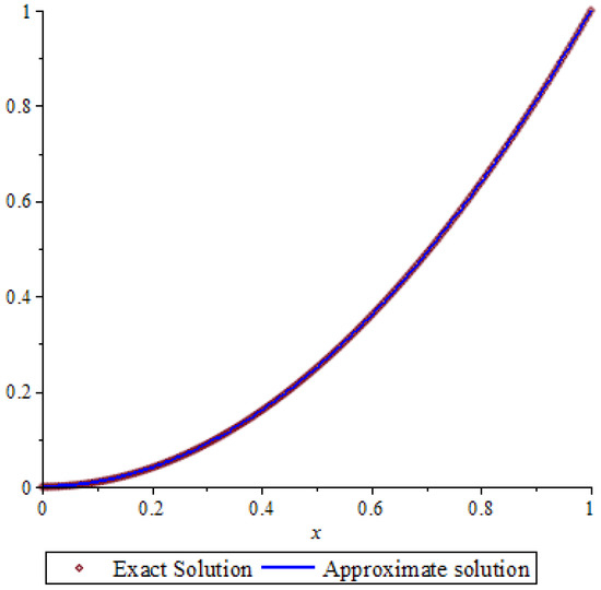
Figure 1.
The approximate solution for .
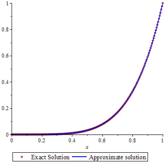
Figure 2.
The approximate solution for .
8. Conclusions
The purpose of this work was to develop an efficient projection method and to analyze its convergence for a fractional-order Bagley–Torvik system. We employed fractional shifted Legendre polynomials as the basis for our development. Two significant advantages exist with the proposed method. We began by converting the problem into a system of two separable fractional-order Bagley–Torvik equations, which we then solved using the present method. Second, approximate solutions were obtained by solving two linear equation systems. To demonstrate the method’s accuracy and performance, numerical results are provided. The current method can be updated to use polynomials other than Legendre’s polynomials. In the future, we will investigate this problem using a family of fractional Chebyshev polynomials.
Author Contributions
Conceptualization, S.A. and A.M.; Methodology, S.A. and A.M.; Investigation, S.A. and A.M.; Resources, S.A. and A.M.; Data curation, S.A. and A.M.; Writing—original draft preparation, S.A. and A.M.; writing—review and editing, S.A. and A.M.; supervision, S.A. and A.M.; funding acquisition, S.A.; Writing—original draft, S.A. and A.M.; Writing—review, S.A. and A.M. All authors have read and agreed to the published version of the manuscript.
Funding
The research of the first author was funded by Taif University Researchers Supporting Project number (TURSP-2020/320), Taif University, Taif, Saudi Arabia.
Institutional Review Board Statement
Not applicable.
Informed Consent Statement
Not applicable.
Data Availability Statement
Not applicable.
Acknowledgments
The authors would like to thank the reviewers and the editor for their insightful comments and suggestions, which significantly improved this original manuscript.
Conflicts of Interest
The authors declare no conflict of interest.
References
- Bagley, R.L.; Torvik, P.J. On the appearance of the fractional derivative in the behavior of real materials. ASME Trans. J. Appl. Mech. 1984, 51, 294–298. [Google Scholar]
- López-Rentería, J.A.; Aguirre-Hernández, B.; Fernández-Anaya, G. LMI stability test for initialized fractional order control systems. Appl. Comput. Math. 2019, 18, 50–61. [Google Scholar]
- López-Rentería, J.A.; Aguirre-Hernández, B.; Fernández-Anaya, G. A new guardian map and boundary theorems applied to the stabilization of initialized fractional control systems. Math. Methods Appl. Sci. 2022, 45, 7832–7844. [Google Scholar] [CrossRef]
- Dehghan, R. A numerical solution of variable order fractional functional differential equation based on the shifted Legendre polynomials. SeMA J. 2019, 76, 217–226. [Google Scholar] [CrossRef]
- Mokhtary, P. Numerical treatment of a well-posed Chebyshev Tau method for Bagley-Torvik equation with high-order of accuracy. Numer. Algor. 2016, 72, 875–891. [Google Scholar] [CrossRef]
- Rahimkhani, P.; Ordokhani, Y. Application of Müntz–Legendre polynomials for solving the Bagley–Torvik equation in a large interval. SeMA J. 2018, 75, 517–533. [Google Scholar] [CrossRef]
- Ji, T.; Hou, J.; Yang, C. Numerical solution of the Bagley-Torvik equation using shifted Chebyshev operational matrix. Adv. Differ. Equ. 2020, 2020, 648. [Google Scholar] [CrossRef]
- Diethelm, K.; Ford, J. Numerical Solution of the Bagley-Torvik Equation. BIT Numer. Math. 2002, 42, 490–507. [Google Scholar] [CrossRef]
- Setia, A.; Liu, Y.; Vatsala, A.S. The Solution of the Bagley-Torvik Equation by Using Second Kind Chebyshev Wavelet. In Proceedings of the 11th International Conference on Information Technology: New Generations, Las Vegas, NV, USA, 7–9 April 2014; pp. 443–446. [Google Scholar] [CrossRef]
- Mennouni, A. A projection method for solving Cauchy singular integro-differential equations. Appl. Math. Lett. 2012, 25, 986–989. [Google Scholar] [CrossRef] [Green Version]
- Mennouni, A. Airfoil polynomials for solving integro-differential equations with logarithmic kernel. Appl. Math. Comput. 2012, 218, 11947–11951. [Google Scholar] [CrossRef]
- Samko, S.G.; Kilbas, A.A.; Marichev, D.I. Fractional Integrals and Derivatives: Theory and Applications; Gordon and Breach Science Publishers: Yverdon, Switzerland, 1993. [Google Scholar]
- Mennouni, A. A new efficient strategy for solving the system of Cauchy integral equations via two projection methods. Transylv. J. Math. Mech. 2022, 14, 63–71. [Google Scholar]
- Mohammadi, F.; Mohyud-Din, S.T. A fractional-order Legendre collocation method for solving the Bagley-Torvik equations. Adv. Differ. Equ. 2016, 2016, 269. [Google Scholar] [CrossRef] [Green Version]
Publisher’s Note: MDPI stays neutral with regard to jurisdictional claims in published maps and institutional affiliations. |
© 2022 by the authors. Licensee MDPI, Basel, Switzerland. This article is an open access article distributed under the terms and conditions of the Creative Commons Attribution (CC BY) license (https://creativecommons.org/licenses/by/4.0/).