Abstract
In order to extract the valuable information from massive and usually unstructured datasets, increasingly, a novel nonparametric approach is proposed for detecting early signs of structural deterioration in civil infrastructure systems from vast field-monitoring datasets. The process adopted six-sample sliding window overtime at one-hour time increments to overcome the fact that the sampling times were not precisely consistent at all monitoring points. After data processing by this method, the eigenvalues and eigenvectors were obtained for each moving window, and then an evaluation index was constructed. Monitored tunnel data were analyzed using the proposed method. The required information extracted from an individual moving window is represented by a set of principal components, which become the new orthogonal variables. The resulting evaluation indicator was strongly correlated with measured and calculated values up to 0.89, even for tiny monitoring datasets. Experiments have verified the rationality and effectiveness of the algorithm, which provides a reference for the application of the method in the monitoring data processing.
1. Introduction
The current condition of operating tunnels is monitored by various agencies, and continually advancing monitoring techniques are widely used in tunnel engineering and geo-engineering. Globally, most medium and long tunnels are equipped with structural monitoring systems to ensure the tunnel’s safety; these include technologically advanced methods such as machine vision and monitoring through measurement reference networks [1,2]. However, commonly in practice, the monitoring system cannot efficiently use the recorded data—for instance, if it does not include intelligent analysis or other capabilities [3].
Displacement and deformation monitoring systems have been used to judge the stability of the rock surrounding tunnels, and fitted algorithms have been developed to measure the deformation of the rock and supporting structures. The movement of the soil and liner displacement between tunnels was analyzed and discussed, and the importance of a tunnel’s efficient data management being equipped with an information system was emphasized [4,5,6,7,8]. Sun et al. [9] developed a high-precision multi-point optical grating displacement monitoring technique that has subsequently been widely used in physical model tests (e.g., [10,11]).
Convergence monitoring systems comprising several measuring points with laser-ranging sensors have been reported, but the measured precision was not always assured. Farahani et al. [12] used 3D laser coupled technology and the digital imaging systems to monitor tunnel deformation and establish tunnel contour models. As digital image correlation (DIC) systems need to be installed in front of the suspect region, however, the practical value was poor in actual tunnels. Kallinikidou et al. [13] reported an analysis of a monitoring database of the Vincent Thomas Bridge’s structural health. However, it is questionable whether this algorithm’s calculation scheme and accuracy are appropriate for tunnels.
A novel monitoring method based on “on-site visualization” (OSV) was proposed by Izumi et al. [14] to conduct real-time data processing. In particular, they addressed the limitations of OSV in cases of incomplete coverage of construction-site accident monitoring. They considered the need to improve the reliability of the power supply to the equipment and how to take equipment failure into account.
In the present study, “data-driven” refers to the implementation of various valuable features such as forecasting, monitoring, evaluation, diagnosis, decision making, scheduling, and optimization based on continuously updated data (Salami et al. [15]). The rapid progress in big data-driven technology and associated software for extracting information from massive and usually unstructured datasets increasingly compensates for the defects cited above. He et al. [16] reported, using computer intelligence technology to compare and analyze the predictive capabilities of the support vector machine, a wavelet neural network and Gaussian process (GP) to determine deformation sequences in the rock surrounding underground openings. They concluded that, of these approaches, GP provides the best predictions. An automatic, highly accurate real-time wireless tunnel deformation monitoring system based on machine-vision and laser technology was proposed by Qiu et al. [17] for predicting tunnel collapse accidents. The system is also suitable for monitoring in low-visibility tunnels.
Examples of proposed extensive data-driven monitoring in non-geotechnical contexts include a modeling strategy proposed by Wang et al. [18] for optimizing BioH2 production during dark fermentation. Chronological multiphase partition analysis and differential monitoring technology are used in a proposed uneven-duration process monitoring scheme for batch processes based on the sequential moving principal component analysis (Guo and Zhang, [19]).
Related to all of these, Shlens et al. [20] explained the working method and procedures of principal component analysis (PCA) using fundamental mathematical cognition. Yun et al. [21] developed a data-driven monitoring framework based on PCA, which they used in various mine monitoring applications to determine the effect of nearby tunnels on the monitored tunnel. Harley and Moura [22] used data-driven matching field processing technology to significantly reduce the positioning error and improve the resolution of structural health monitoring systems. He et al. [23] proposed a flexible, robust PCA method that uses two matrices for error correction, one of which obtains data representation to improve performance and practicability.
Long-term deformation monitoring systems for tunnels accumulate enormous datasets that are difficult to analyze and process in a way that reflects the deformation of the tunnel in real-time. Google GFS, MapReduce, and Impala based on Hadoop (real-time) are variously used for big data processing (Isard et al., [24]; Leibiusky et al., [25]). Xiang et al. [26] proposed a design and optimization method for an extensive data processing system based on orthogonal decomposition, which has the advantage of performing efficient and hierarchical calculations such that the primary target and secondary factors are interlayered, and the primary target is prioritized. It dramatically accelerates the processing of large datasets and improves its efficiency (Li et al. [27]; Li et al. [28]; Suzuki et al. [29]).
The abovementioned deformation monitoring methods are essentially parametric approaches to the problem. They, therefore, suffer from limitations, such as unknown structural characteristics, unknown material properties, and the strange behavior of the surrounding rock. Precisely, the responses are measured using a range of sensors, and no input information is obtained. It may prevent the verification of the correctness of the model, so such approaches do not necessarily reflect the actual structural failure progression. By contrast, nonparametric approaches do not suffer from these drawbacks, making them more feasible for analyzing the large datasets accumulated during monitoring.
This study reviews recent developments in nonparametric approaches, and a data-driven detection model is proposed for long-term deformation monitoring of an operational tunnel adopting the orthogonal decomposition approach.
2. Site Description and Engineering Background
Long-term deformation monitoring was carried out at a light subway tunnel retrofit project in Chongqing, China. Horizontal and vertical displacements, structural stress, structural fractures, and settlement of the track-bed and rail structure were monitored at a location between the rail platform and the station. Comprehensive analysis of the impact on the structure and operational safety of the subway was the basis for the decision making of the safe operation of the rail transit system.
The monitoring system comprised an independent coordinate system with eight reference points (two at each end of the left- and right-hand tunnels) set at each end of the interval to be monitored and inside the hazardous area affected by construction. The coordinates of all eight reference points were the reference data for the entire monitoring system. Work base points 300–600 m apart were arranged at appropriate positions inside the tunnel and within the interval to be monitored. Precision wires between the reference and work base point served as the first-level control network. A measuring robot automatically and accurately aligned the operational base or reference point. It used quasi-stable adjustment to calculate the precise coordinates and elevation of the station in real-time to monitor each point. The cross-section of the monitoring tunnel is shown in Figure 1.
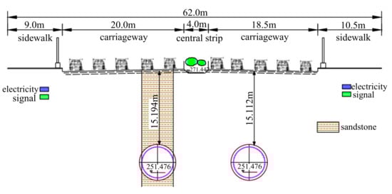
Figure 1.
Cross-section of monitoring tunnel.
Each displacement monitoring section contained one arch-top settlement monitoring point, two arch waist settlement monitoring points (also used as horizontal convergence monitoring points), and two points for monitoring the track-bed settlement. Each stress monitoring section contained three stress/strain monitoring points. The arrangement of the measuring points is shown in Figure 2.
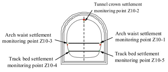
Figure 2.
Arrangement of measuring points inside the tunnel at Section Z10.
There were seven underground passages within the monitoring interval, with twenty-one deformation monitoring sections in the left-hand tunnel and forty-two in the right-hand tunnel. A stress/strain monitoring section comprising three monitoring points was located in the central area of the surface passage. In total, 14 stress/strain monitoring sections were located not more than 100 m apart in the left-hand and right-hand tunnel, and 42 deformation monitoring sections were located in each. Overall, 82 displacement monitoring sections and 14 stress/strain monitoring sections were positioned in the tunnels in this project. The track-bed and arch point arrangement images are shown in Figure 3.
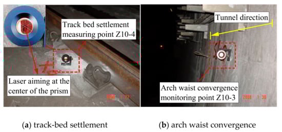
Figure 3.
Measurement points: (a) track-bed settlement and (b) arch waist convergence.
3. Continuous Monitoring of Tunnel Deformation
The monitoring system was commissioned on 14 March 2015 and the first monitoring round was completed on 16 March. Automatic deformation monitoring was conducted every two hours. The average of the observations for each round was considered the daily observation. The monitoring during the construction period began on 26 December 2014 and ended on 4 January 2016; the monitoring of the operational period commenced in January 2016 and ceased in December 2017. Monitoring during the operational period was carried out fortnightly, monthly, and once every two months in the first, second, third, and fourth quarters of 2016. After long-term monitoring, gross errors in the recorded observations were eliminated to obtain accurate and reliable data for tunnel deformation analysis.
The recorded data were grouped into primary divisions to obtain the time–displacement relationships for the five monitoring points at monitoring sections Z10, Z11, Z12, and Z13. Figure 4 and Figure 5 show the displacement variation with time at Sections Z10 and Z11.
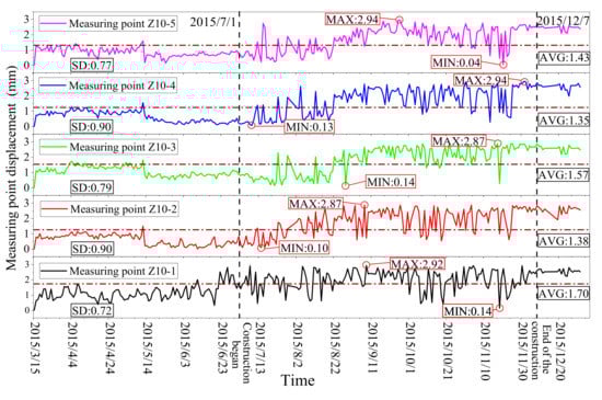
Figure 4.
Time–deformation displacement of light rail line at monitoring section Z10.
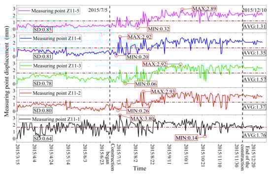
Figure 5.
Time–deformation displacement of light rail line at monitoring section Z11.
Figure 4 and Figure 5 show that the displacements of the measurement point at the vault of the section fluctuated significantly when the track above it was under construction, indicating a large settlement deformation at the tunnel vault. As track construction neared completion, settlement deformation tended to stabilize, showing fewer fluctuations and smaller peak values. The deformations at the track-bed and both sides of the arch waist fluctuated similarly. Long-term monitoring showed relatively stable deformation with no significant fluctuations.
Monitoring progressed from Z10 to Z11, 20 m apart (Benchmark no. DK0+637 for Section Z10; benchmark no. DK0+657 for Section Z11). It is clear in Figure 4 that large displacement variations at section Z10 began on 1 July 2015 (commencement of track construction work) and ended on 7 December 2015 when construction work ceased. Displacements fluctuated between 2.94 and 0.04 mm (average 1.70 mm; standard deviation 0.90 mm). Similarly, Figure 5 shows large displacement variations at section Z11 corresponding to the period of track construction work from 5 July to 10 December 2015. Displacements fluctuated between 3.80 and 0.06 mm (average 1.76 mm; standard deviation 0.85 mm). Figure 6 and Figure 7 show displacement vs. time at sections Z12 and Z13, 80 m apart (Benchmark no. DK0+737 for Section Z12; benchmark no. DK0+817 for Section Z13).
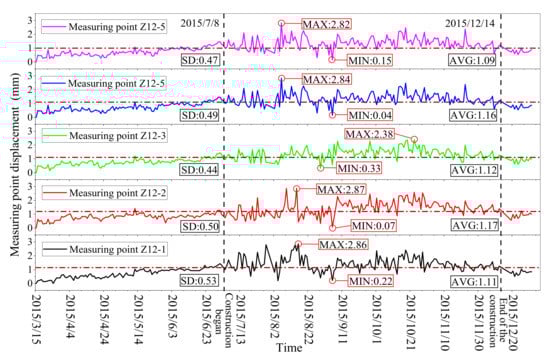
Figure 6.
Time–deformation displacement of light rail line at monitoring section Z12.
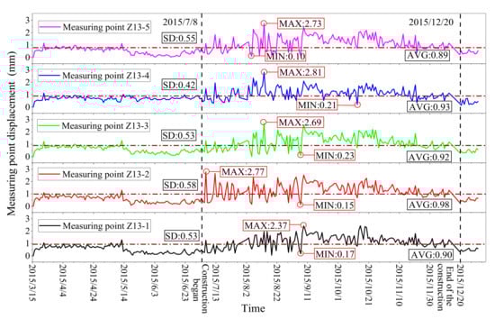
Figure 7.
Time–deformation displacement of light rail line at monitoring section Z13.
Monitoring activity progressed from Z12 towards Z13. Figure 6 and Figure 7 show significant, abrupt deformation changes at sections Z12 and Z13, corresponding with the period of track construction overhead (8 July–14 December 2015 for Z12, and 8 July–20 December 2015 for Z13). At section Z12, displacement fluctuated between 0.04 and 2.87 mm (average 1.17 mm; standard deviation 0.53 mm), and from 0.10 to 2.81 mm at section Z13 (average 0.98 mm; standard deviation 0.58 mm). These indicate that the long-term monitored displacements at sections Z12 and Z13 were highly accurate and sensitive, and few errors were apparent.
4. Fundamentals of Principal Component Analysis and Singular Value Decomposition Method
The following review of nonparametric approaches for tunnel structure analysis includes some implications for resolving the challenges. Proper orthogonal decomposition (POD) methods are increasingly adopted in engineering contexts. In data analysis, POD is a powerful and elegant method to obtain low-dimensional approximations of high-dimensional processes. The main objective of POD is to seek ordered orthonormal basis vectors within a subspace.
4.1. The Basic Principle of Principal Component Analysis
The purpose of PCA is usually to identify the structure of multivariate stochastic observations, either by variance maximization or least mean squares techniques. The POD method based on PCA is described below.
Assuming that is a random vector and X is the original dataset, each X column is a single sample. PCA is a linear combination of its primary vectors to the revealed internal law of the data. Consider Y an matrix related by the linear transformation P, and Y is a new representation of the original dataset X.
This is defined as:
PX = Y
Consider P a rotation and stretch tensor, and P is a matrix which transforms X into Y. The columns of X are expressed by the rows of P:
Without a loss of generality, the 1st, 2nd,…, mth principal components are . The first principal component yi is a linear combination of each element of the original random vector. That is,
where is a constant vector.
By introducing the Lagrangian multiplier , we obtain
Differentiating both sides of Equation (5) with respect to , gives
If the right-hand side of Equation (6) is zero, then the equation can be simplified as
where is the eigenvalue and is the corresponding eigenvector of the covariance matrix . Multiplying both sides of Equation (7) by gives
Note that must be as large as possible since it was selected as the maximum eigenvalue of . Similarly, the second principal component is obtained from
where is . Multiplying both sides of Equation (10) by gives
Note that is selected as the second eigenvalue of , such that .
The principal components, which are uncorrelated and unordered, closely retain the variation in the original dataset. In particular, the first several principal components retain almost all the variation in all the original variables, and the first principal component y1 is uncorrelated with the second principal component y2.
Redundant cases are readily identified in the two-variable case by means of the best-fit line slope. For instance, for Sets A and B,
Thus, the variances of A are defined as:
The variances of B are defined as:
Considering the degree of linearity of the relationship between A and B, the covariance function is given by
where the degree of redundancy is the magnitude or absolute value of . A positive value of denotes positively correlated data, and vice versa. In particular, only if A and B are uncorrelated, then = 0.
Without a loss of generality, it is generalized to an arbitrary number; that is, a new m × n matrix X and row vectors is defined by
Therefore, the CX represents the covariance matrix and is defined as
where CX is a square symmetrical m × m matrix, the variance of particular measurement types, and the covariance between measurement types, are the diagonal and off-diagonal terms of CX, respectively. In this study, the covariance values reflected the redundancy of measurements.
4.2. Singular Value Decomposition Method
The dataset X is an m × n matrix, where . The sampling number is n and the number of sampling types is m. Therefore, when the number of samplings is greater than the sampling types, let
where represent n samples.
To obtain the principal components of X, two objectives should be fulfilled: CY is a diagonal matrix, and the matrix P in Y = PX is an orthonormal matrix. The expression for CY is
Substituting PX into Equation (20) gives
For any symmetrical matrix A, there is a diagonal matrix D and a matrix E of eigenvectors of A arranged as columns, such that and each row of matrix P is an eigenvector of , such that CY may be written as
To summarize, the variance of X along with pi is the ith diagonal value of CY, and the eigenvectors of CX are the principal components of X.
Let the eigenvalues of be arranged in a decreasing order:
The singular values of are , where
Generally, there are orthonormal or base sets of eigenvectors and in the dimensional space. For a new diagonal matrix, is given by
The rank-ordered set of singular values is . The accompanying orthogonal matrices are constructed as
Matrix V is orthogonal, so Equation (26) may be rewritten in the form
For any arbitrary matrix X, it can be converted into an orthogonal matrix, another orthogonal matrix, and a diagonal matrix.
5. Model Construction Using Data-Driven Analysis
Monitored data were recorded in stages, so that sampling times were not precisely consistent at all monitoring points. The proposed method for analyzing the tunnel deformation dataset adopted six-sample sliding window overtime at one-hour time increments to overcome this limitation. After data processing, the eigenvectors and eigenvalues were obtained for each moving window.
The proposed model adopted the spectral proper orthogonal decomposition (SPOD) approach (described step by step below) for the sampling sequence at each monitoring point [30,31,32]. Then an evaluation index was constructed from the datasets.
Step 1 (data matrix): the data matrix , where i is the number of samples and j is the number of measurement types, is sliced in the direction of increasing data.
Step 2 (determining the moving window): A ‘moving window’ is a sample clip of a fixed amount of monitoring data. It is written Wi,j where = 1, 2, …, n (window size), and j is the number of measurement types.
Step 3 (efficient moving mechanism): The moving window moves in steps with a fixed number of samples on matrix X to obtain the moving matrix Wk,j. An example of a moving window is:
After the following new sample is added, the current moving window slices in the direction of the added data to form a new moving window.
Step 4 (forming an evaluating indicator): For each moving window Wk,j, the model was established by the POD method. The evaluating indicator k is given by
where is the first eigenvalue and is the sum of all eigenvalues.
6. Results of Monitoring Data Analysis
6.1. Dataset Matrix of Real-Time Monitoring Data
This section evaluates the proposed method and compares it with previous methods at different monitoring stages. The evaluation was performed for four datasets to confirm the effectiveness of the proposed method. The datasets represent displacements in the x-, y-, and z-directions in the tunnel wall, extracted from five monitoring points in each case. The SPOD procedure was then conducted for a six-sample moving window at one-hour intervals. The detailed compositions of the evolving indices in the moving window are listed in Table 1.

Table 1.
Composition of evolution index.
6.2. Discussion and Analysis of Real-Time Monitoring Data
Each moving window was decomposed by the SPOD algorithm, then the eigenvalues () and eigenvectors (V) of each dataset were obtained for each moving window.
6.2.1. Monitored Results at Section 10
Figure 8 shows the changes of deformation at the measurement date and eigenvalues at point 1, Section 10 (Z10-1).
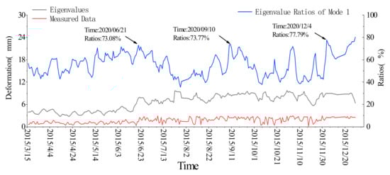
Figure 8.
Deformation time histories of the tunnel lining and first principal component at monitoring point Z10-1. See Appendix A for Z10-2–Z10-5 results.
See Appendix A, Figure A1, Figure A2, Figure A3 and Figure A4, for corresponding details for points Z10-2 to Z10-5.
The magnitude of the normalized eigenvector is measured by the eigenvalue, as described in Equation (27). For each moving unit, Mode 1 was the dominant mode during the monitoring period (). No significant change was observed in the eigenvalue ratios of Mode 1 as the tunnel was not noticeably affected by construction during that period. It then showed a significant decrease and increase on 21 June and 1 August, and increased to 0.7377 on 10 September. Subsequently, it firstly decreased then increased. The maximum ratio of 0.7779 was recorded on 4 December 2015.
The eigenvalue ratios of Mode 1 for monitoring point Z10-2 were 0.7315, 0.7354, and 0.81 on 19 May, 10 September, and 2 December 2015, respectively. No significant change was observed in the eigenvalue ratios of Mode 1 from 15 March to 19 May, as the tunnel was not noticeably affected by construction, but showed a significant decrease on 19 May and increase on July 20. The eigenvalue ratio of Mode 1 increased to 0.7354 on 10 September, followed firstly by a decrease, then an increase. The maximum ratio of 0.81 was observed on 2 December 2015.
The peak values in the ratio curves of Z10-2, Z10-3, and Z10-4 (Figure A1, Figure A2 and Figure A3) appear about two months before Z10-1 (Figure 8) and Z10-5 (Figure A4), when the construction work was taking place closest to the left-hand side of the tunnel. The recorded changes at the monitoring section Z10 were probably due to the effect of construction.
6.2.2. Monitored Results at Section 11
Figure 9 shows the monitoring results for monitoring point 1 at Section 11 (Z11-1).
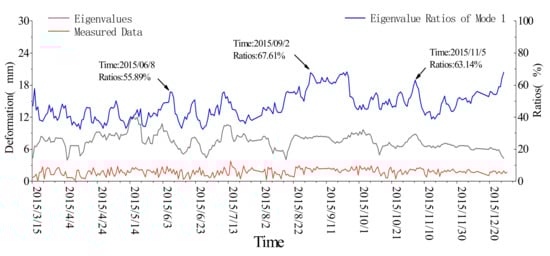
Figure 9.
Deformation time histories of tunnel lining and first principal component at monitoring point Z11-1. See Appendix B for Z11-2–Z11-5 results.
No significant change was observed from 15 March to 30 May, as the tunnel was not noticeably affected by construction. The values showed a significant decrease and increase on 30 May and 20 July, respectively, and reached 0.7883 on 9 September, followed by a decrease and then an increase. The maximum ratio of 0.8072 was observed on 27 November.
The peak values in the ratio curves of Z11-2, Z11-3, and Z11-4 appear ahead of Z11-1 and Z11-5 (see Appendix B) by approximately one week, probably because the construction area was near the left-hand side of the tunnel.
6.2.3. Monitored Results at Section 12
As shown in Figure 10, the peak eigenvalue ratios of Mode 1 of Section 12 (Z12-1) were 0.8151, 0.8535, 0.8584, 0.8492, and 0.8084, respectively, on 5 June, 4 June, 4 June, 1 June, and 30 May, at the various monitoring points.
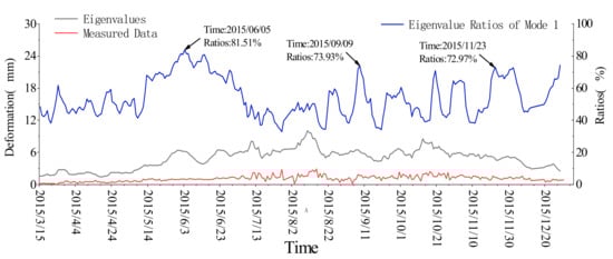
Figure 10.
Deformation time histories of tunnel lining and the first principal component at monitoring point Z12-1. See Appendix C for Z12-2–Z12-5 results.
The peak eigenvalue ratios of Mode 1 of Section 12 (Z12-1) was observed on 5 June. The result shows that the peak value of Section 12 (Z12-1) occurred three days before Section 11 (Z11-1). It is found that the closer the monitoring points were to the displacement-affected zone, the larger the peak response was.
6.2.4. Monitored Results at Section 13
Figure 11 shows the Mode 1 eigenvalue ratios and relevant dates for Section 13. The eigenvalue ratios of Mode 1 for monitoring point Z13-1 were 0.8303, 0.7581, and 0.7198 on 4 June, 9 September, and 24 November 2015, respectively. The peak value of Mode 1 for monitoring point Z13-1 decreases gradually, attributable to the effect of the redistribution of the surrounding rock pressure. All the values were greater than 0.7, which tends to confirm the high sensitivity of the proposed method.
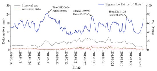
Figure 11.
Deformation time histories of tunnel lining and the first principal component at monitoring point Z13-1. See Appendix D for Z13-2–Z13-5 results.
6.3. Comparison with Traditional Analytical Method
To improve the precision of analysis in conventional geotechnical engineering approaches to assess or predict tunnel deformation, it is usually necessary to have as much information available about the relevant variables as possible, including their minimum and mean values and standard deviation.
The orthogonal decomposition method was employed for processing large datasets in this study of monitoring the deformation of operational tunnels. The results shown in Figure 8, Figure 9, Figure 10 and Figure 11 and Appendix A, Appendix B, Appendix C, Appendix D demonstrate that the proposed method adequately interprets the monitoring data. The Mode 1 eigenvalue ratios were found to be highly sensitive to fluctuations in tunnel deformation in all cases.
This finding may provide insight into the phenomenon that higher eigenvalue ratios are valuable indicators of value fluctuations in large monitoring datasets.
7. Conclusions
In tunnel monitoring systems and associated geotechnical engineering activities, it is crucial to extract helpful information from the vast datasets generated by tunnel displacement monitoring to evaluate the current performance of the tunnel. The task of analyzing and managing tunnel deformation data is the core of the long-term deformation monitoring of operating tunnels.
This study proposes an orthogonal decomposition method to construct a data processing model for datasets from current tunnel monitoring methods. As discussed in Section 2, the actual monitoring process was studied by considering four groups of five monitoring points, each of which collected tunnel deformation data over the same 10-month period. The SPOD technique analyzed the datasets in which observations were described using several intercorrelated quantitative dependent variables. The goal of this technique was to extract meaningful information from vast amounts of raw data.
Subsequently, the information was represented as a set of principal components that were new orthogonal variables. The quality was evaluated using cross-validation techniques. Additionally, data fusion processing was performed on the data to make them more detailed, intelligent, and accurate.
In order to confirm the feasibility and effectiveness of the proposed method on the four datasets, each moving unit was decomposed and its principal features were extracted by the proposed algorithm. For each monitored period, four sets of eigenvectors and eigenvalues were obtained using Scikit-learn machine learning tools. The experimental results show that the evaluating k was between 0.7065 and 0.8888. The proposed algorithm revealed the changes and trends of the critical variables in tunnel deformation monitoring. Such methods will help achieve the goal of the early detection of possible structural deterioration.
Author Contributions
Conceptualization, R.X.; methodology, R.X.; software, Z.Y.; validation, Z.L.; formal analysis, P.X.; investigation, B.S.; resources, Y.Y.; data curation, Z.Y.; writing—original draft preparation, R.X.; writing—review and editing, R.X.; supervision, P.X.; project administration, R.X. All authors have read and agreed to the published version of the manuscript.
Funding
This research was funded by the Major Program of the National Natural Science Foundation of China (Grant No. 51991394), the Chongqing Nature Science Foundation (Grant No. cstc2019jcyj-msxmX0600), and the State Key Laboratory of Mountain Bridge and Tunnel Engineering Fund Project (Award No. SKLBT-19-013) for funding this research.
Institutional Review Board Statement
Not applicable.
Informed Consent Statement
Informed consent was obtained from all subjects involved in the study.
Data Availability Statement
The sample data collection sheet, the data used for analysis, and the associated computer programs can be made available on request from the corresponding author.
Acknowledgments
The authors gratefully acknowledge the support extended by the Major Program of the National Natural Science Foundation of China (Grant No. 51991394), the Chongqing Nature Science Foundation (Grant No. cstc2019jcyj-msxmX0600), and the State Key Laboratory of Mountain Bridge and Tunnel Engineering Fund Project (Award No. SKLBT-19-013) for funding this research.
Conflicts of Interest
The authors declare no conflict of interest.
Appendix A
The changes of deformation and eigenvalues at the measurement date for points 2–5, Section 10, and the left-hand tunnel are shown in Figure A1, Figure A2, Figure A3 and Figure A4.
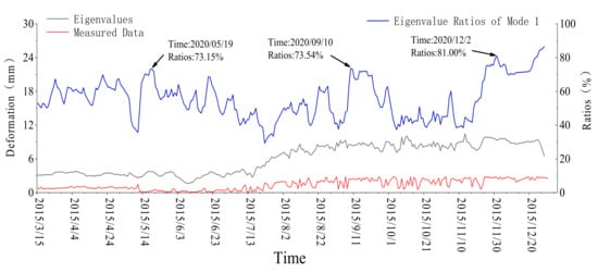
Figure A1.
Deformation time histories of the tunnel lining and first principal component at monitoring point Z10-2.
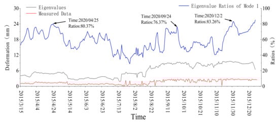
Figure A2.
Deformation time histories of the tunnel lining and first principal component at monitoring point Z10-3.
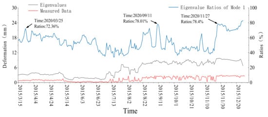
Figure A3.
Deformation time histories of the tunnel lining and first principal component at monitoring point Z10-4.
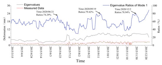
Figure A4.
Deformation time histories of the tunnel lining and first principal component at monitoring point Z10-5.
Appendix B
The changes of deformation and eigenvalues at the measurement date for points 2–5, Section 11, and the left-hand tunnel are shown in Figure A5, Figure A6, Figure A7 and Figure A8.
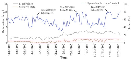
Figure A5.
Deformation time histories of the tunnel lining and first principal component at monitoring point Z11-2.

Figure A6.
Deformation time histories of the tunnel lining and first principal component at monitoring point Z11-3.
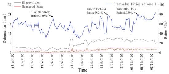
Figure A7.
Deformation time histories of the tunnel lining and first principal component at monitoring point Z11-4.
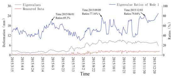
Figure A8.
Deformation time histories of the tunnel lining and first principal component at monitoring point Z11-5.
Appendix C
The changes of deformation and eigenvalues at the measurement date for points 2–5, Section 12, and the left-hand tunnel are shown in Figure A9, Figure A10, Figure A11 and Figure A12.
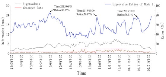
Figure A9.
Deformation time histories of the tunnel lining and first principal component at monitoring point Z12-2.
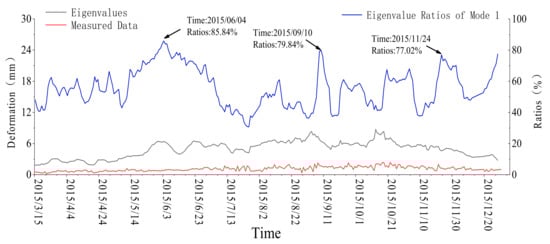
Figure A10.
Deformation time histories of the tunnel lining and first principal component at monitoring point Z12-3.
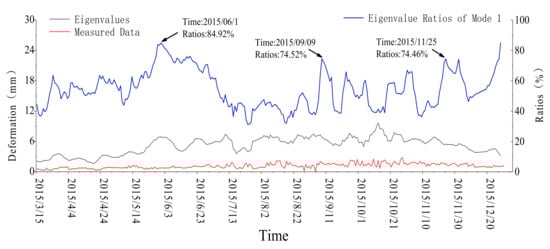
Figure A11.
Deformation time histories of the tunnel lining and first principal component at monitoring point Z12-4.
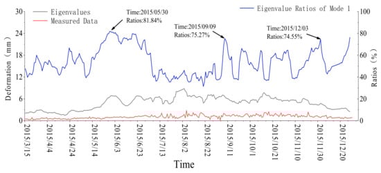
Figure A12.
Deformation time histories of the tunnel lining and first principal component at monitoring point Z12-5.
Appendix D
The changes of deformation and eigenvalues at the measurement date for points 2–5, Section 13, and the left-hand tunnel are shown in Figure A13, Figure A14, Figure A15 and Figure A16.
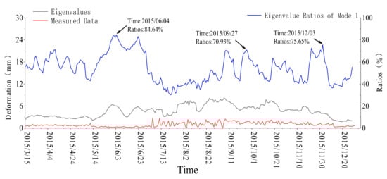
Figure A13.
Deformation time histories of the tunnel lining and first principal component at monitoring point Z13-2.
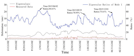
Figure A14.
Deformation time histories of the tunnel lining and first principal component at monitoring point Z13-3.
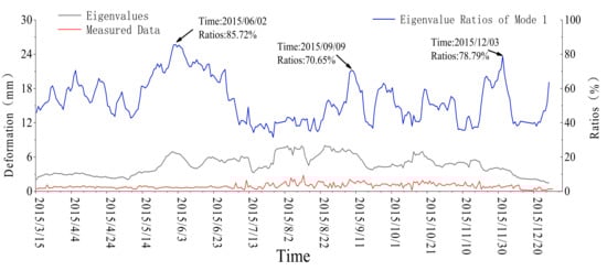
Figure A15.
Deformation time histories of the tunnel lining and first principal component at monitoring point Z13-4.
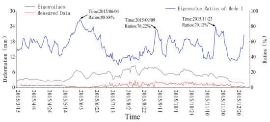
Figure A16.
Deformation time histories of the tunnel lining and first principal component at monitoring point Z13-5.
References
- Bryn, M.Y.; Afonin, D.A.; Bogomolova, N.N.; Nikitchin, A.A. Monitoring of transport tunnel deformation at the construction stage. Procedia Eng. 2017, 189, 417–420. [Google Scholar] [CrossRef]
- Ding, L.Y.; Zhou, C.; Deng, Q.X.; Luo, H.B.; Ye, X.W.; Ni, Y.Q.; Guo, P. Real-time safety early warning system for cross passage construction in Yangtze Riverbed Metro Tunnel based on the internet of things. Autom. Constr. 2013, 36, 25–37. [Google Scholar] [CrossRef]
- Zhou, J.; Xiao, H.; Jiang, W.; Bai, W.; Liu, G. Automatic subway tunnel displacement monitoring using robotic total station. Measurement 2020, 151, 107251. [Google Scholar] [CrossRef]
- Chen, J.F.; Kang, C.Y.; Shi, Z.M. Displacement monitoring of parallel closely spaced highway shield tunnels in marine clay. Mar. Georesour. Geotechnol. 2015, 33, 45–50. [Google Scholar] [CrossRef]
- Rabensteiner, K.; Chmelina, K. Tunnel monitoring in urban environments. Geomech. Tunn. 2016, 9, 23–28. [Google Scholar] [CrossRef]
- Scaioni, M.; Barazzetti, L.; Giussani, A.; Previtali, M.; Roncoroni, F.; Alba, M.I. Photogrammetric techniques for monitoring tunnel deformation. Earth Sci. Inform. 2014, 7, 83–95. [Google Scholar] [CrossRef]
- Shimizu, N.; Tayama, S.; Hirano, H.; Iwasaki, T. Monitoring the ground stability of highway tunnels constructed in a landslide area using a web-based GPS displacement monitoring system. Tunn. Undergr. Space Technol. 2005, 21, 266–267. [Google Scholar] [CrossRef]
- Walton, G.; Delaloye, D.; Diederichs, M.S. Development of an elliptical fitting algorithm to improve change detection capabilities with applications for deformation monitoring in circular tunnels and shafts. Tunn. Undergr. Space Technol. 2014, 43, 336–349. [Google Scholar] [CrossRef]
- Sun, S.; Li, S.; Li, L.; Shi, S.; Zhou, Z.; Gao, C. Design of a displacement monitoring system based on optical grating and numerical verification in geomechanical model test of water leakage of tunnel. Geotech. Geol. Eng. 2018, 36, 2097–2108. [Google Scholar] [CrossRef]
- Hu, J.; Li, S.; Shi, S.; Zhang, J.; Guo, X. Development and application of a model test system for rockfall disaster study on tunnel heading slope. Environ. Earth Sci. 2019, 78, 1–14. [Google Scholar] [CrossRef]
- Zhu, G.; Feng, X.; Zhou, Y.; Li, Z.; Fu, L.; Xiong, Y. Physical model experimental study on spalling failure around a tunnel in synthetic marble. Rock Mech. Rock Eng. 2020, 53, 909–926. [Google Scholar] [CrossRef]
- Farahani, B.V.; Barros, F.; Sousa, P.J.; Cacciari, P.P.; Tavares, P.J.; Futai, M.M.; Moreira, P. A coupled 3D laser scanning and digital image correlation system for geometry acquisition and deformation monitoring of a railway tunnel. Tunn. Undergr. Space Technol. 2019, 91, 102995. [Google Scholar] [CrossRef]
- Kallinikidou, E.; Yun, H.B.; Masri, S.; Caffrey, J.P.; Sheng, L.H. Application of orthogonal decomposition approaches to long-term monitoring of infrastructure systems. J. Eng. Mech. 2013, 139, 678–690. [Google Scholar] [CrossRef]
- Izumi, C.; Akutagawa, S.; Tyagi, J.; Abe, R. Application of a new monitoring scheme “on site visualization” for safety management on Delhi Metro project. Tunn. Undergr. Space Technol. 2014, 44, 130–147. [Google Scholar] [CrossRef]
- Salami, B.A.; Olayiwola, T.; Oyehan, T.A.; Raji, I.A. Data-driven model for ternary-blend concrete compressive strength prediction using machine learning approach. Constr. Build. Mater. 2021, 301, 124152. [Google Scholar] [CrossRef]
- He, P.; Xu, F.; Sun, S.Q. Nonlinear deformation prediction of tunnel surrounding rock with computational intelligence approaches. Geomat. Nat. Hazards Risk 2020, 11, 414–427. [Google Scholar] [CrossRef] [Green Version]
- Qiu, Z.; Li, H.; Hu, W.; Wang, C.; Liu, J.; Sun, Q. Real-time tunnel deformation monitoring technology based on laser and machine vision. Appl. Sci. 2018, 8, 2579. [Google Scholar] [CrossRef]
- Wang, Y.; Tang, M.; Ling, J.; Wang, Y.; Liu, Y.; Jin, H.; He, J.; Sun, Y. Modeling biohydrogen production using different data driven approaches. Int. J. Hydrog. Energy 2021, 48, 29822–29833. [Google Scholar] [CrossRef]
- Guo, R.; Zhang, N. A process monitoring scheme for uneven-duration batch process based on sequential moving principal component analysis. IEEE Trans. Control Syst. Technol. 2020, 28, 583–592. [Google Scholar] [CrossRef]
- Shlens, J. A Tutorial on Principal Component Analysis; Cornell University: Ithaca, NY, USA, 2014; p. 12. [Google Scholar]
- Yun, H.; Park, S.; Mehdawi, N.; Mokhtari, S.; Chopra, M.; Reddi, L.; Park, K. Monitoring for close proximity tunneling effects on an existing tunnel using principal component analysis technique with limited sensor data. Tunn. Undergr. Space Technol. 2014, 43, 398–412. [Google Scholar] [CrossRef]
- Harley, J.B.; Moura, J.M.F. Data-driven matched field processing for Lamb wave structural health monitoring. J. Acoust. Soc. Am. 2014, 135, 1231–1244. [Google Scholar] [CrossRef] [PubMed]
- He, Z.N.; Wu, J.G.; Han, N. Flexible robust principal component analysis. Int. J. Mach. Learn. Cybern. 2020, 11, 603–613. [Google Scholar] [CrossRef]
- Isard, M.; Budiu, M.; Yu, Y.; Birrell, A.; Fetterly, D. Dryad: Distributed data-parallel programs from sequential building blocks. In Proceedings of the 2nd ACM SIGOPS/EuroSys European Conference on Computer Systems, Lisbon, Portugal, 21–23 March 2007; Association for Computing Machinery: New York, NY, USA; Volume 41, pp. 59–72. [Google Scholar]
- Leibiusky, J.; Eisbruch, G.; Simonassi, D. Getting Started with Storm; O’Reilly: Sebastopol, CA, USA, 2012. [Google Scholar]
- Xiang, X.; Zhao, X.; Liu, Y.; Gong, G.; Zhang, H. An orthogonal decomposition based design method and implementation for big data processing system. J. Comput. Res. Devel. 2017, 54, 1097–1108. [Google Scholar]
- Li, Z.; Ma, Y.; Cao, L.; Wu, H. Uncertainty quantification of proper orthogonal decomposition based online power-distribution reconstruction. Ann. Nucl. Energy 2020, 140, 1–9. [Google Scholar]
- Li, Y.; RazaviAlavi, S.; AubouRizk, S. Data-driven simulation approach for short-term planning of winter highway maintenance operations. J. Comput. Civ. Eng. 2021, 35. [Google Scholar] [CrossRef]
- Suzuki, T.; Chatellier, L.; David, L. A few techniques to improve data-driven reduced-order simulations for unsteady flows. Comput. Fluids 2020, 201, 104455. [Google Scholar] [CrossRef]
- Nidhan, S.; Schmidt, O.; Sarkar, S. Analysis of coherence in turbulent stratified wakes using spectral proper orthogonal decomposition. J. Fluid Mech. 2022, 934, A12. [Google Scholar] [CrossRef]
- Ek, H.; Nair, V.; Douglas, C.; Lieuwen, T.; Emerson, B. Permuted proper orthogonal decomposition for analysis of advecting structures. J. Fluid Mech. 2022, 930, A14. [Google Scholar] [CrossRef]
- Papapicco, D.; Demo, N.; Girfoglio, M.; Stabile, G.; Rozza, G. The Neural Network shifted-proper orthogonal decomposition: A machine learning approach for non-linear reduction of hyperbolic equations. Comput. Methods Appl. Mech. Eng. 2022, 392, 114687. [Google Scholar] [CrossRef]
Publisher’s Note: MDPI stays neutral with regard to jurisdictional claims in published maps and institutional affiliations. |
© 2022 by the authors. Licensee MDPI, Basel, Switzerland. This article is an open access article distributed under the terms and conditions of the Creative Commons Attribution (CC BY) license (https://creativecommons.org/licenses/by/4.0/).